ShadowNav: Autonomous Global Localization for Lunar Navigation in Darkness

Abstract

The ability to determine the pose of a rover in an inertial frame autonomously is a crucial capability necessary for the next generation of surface rover missions on other planetary bodies. Currently, most on-going rover missions utilize ground-in-the-loop interventions to manually correct for drift in the pose estimate and this human supervision bottlenecks the distance over which rovers can operate autonomously and carry out scientific measurements. In this paper, we present ShadowNav, an autonomous approach for global localization on the Moon with an emphasis on driving in darkness and at nighttime. Our approach uses the leading edge of Lunar craters as landmarks and a particle filtering approach is used to associate detected craters with known ones on an offboard map. We discuss the key design decisions in developing the ShadowNav framework for use with a Lunar rover concept equipped with a stereo camera and an external illumination source. Finally, we demonstrate the efficacy of our proposed approach in both a Lunar simulation environment and on data collected during a field test at Cinder Lakes, Arizona.

1 Introduction

Space missions that require long-range autonomous driving on the surface of extra planetary bodies have gained significant interest lately especially for the Lunar surface. For example, in the latest Decadal Survey [National Academies of Sciences, Engineering, and Medicine, 2022b], the Endurance-A Lunar rover was recommended to be implemented as a strategic class mission as the highest priority of the Lunar Discovery and Exploration Program. This mission proposal calls for a $2000\text{\,}\mathrm{km}$ traverse in the South Pole-Aitken (SPA) Basin to collect $100\text{\,}\mathrm{kg}$ of samples for delivery to Artemis astronauts. This mission concept study [Keane et al., 2022] identifies several key capabilities required to complete this mission:

1. Endurance will need to drive 70% of its total distance during the night to enable daytime hours dedicated to science and sampling.

2. The mission will require onboard autonomy for the majority of its operations, while the ground only handles contingencies.

3. Global localization is necessary to maintain an error of $<$$10\text{\,}\mathrm{m}$ relative to orbital maps.

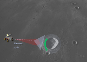
(a)

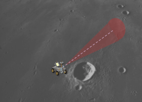
(b)

Figure 1: The ShadowNav concept relies on using crater rims as landmarks. As the rover begins driving (a), its uncertainty in the global frame increases and must be corrected for. By equipping the Lunar rover with a stereo camera and an external illumination source, the leading edges of detected craters (shown in green) are used to associate the crater with known ones from an offline map and decrease the pose uncertainty. As the rover continues to drive, (b) this process repeats intermittently to be able to continue mission operations.

This level of autonomy and drive distance would be an order of magnitude larger than any previous surface mission on an extra planetary body. For example, as the current state-of-the-art in beyond Earth surface autonomy, Mars 2020 has driven $11.6\text{\,}\mathrm{km}$ autonomously over the course of a year and a half and the longest individual autonomous drive was approximately $700\text{\,}\mathrm{m}$ [Verma et al., 2023a]. A key bottleneck that limits longer autonomous drives is the problem of absolute localization, which is the problem of determining the position and orientation of the vehicle in an inertial frame. Without a reliable means of accomplishing autonomous localization autonomously, the vehicle must stop and wait for ground-in-the-loop operators to manually perform absolute localization. In the case of surface rovers used on other planetary bodies, existing relatively localization methods experience approximately 2% drift and this limits autonomous driving to approximately $500\text{\,}\mathrm{m}$ before a manual absolute localization is triggered once the error exceeds $10\text{\,}\mathrm{m}$  [Maimone et al., 2007, Maimone et al., 2022].

Currently however, the entirety of the Lunar surface does not have continuous communication with Earth and having the vehicle wait until communications with the ground station is possible will severely slow down the traverse rates. The lack of frequent absolute localization for the rover would lead to errors greater than the maximum $10\text{\,}\mathrm{m}$ localization error which would present significant risks to the mission through deviations from the desired trajectory. For proposed missions such as Endurance-A, the requirement to drive longer distances on the order of several kilometers a day necessitates the development of an autonomous and performant technique to perform absolute localization onboard the vehicle and without ground-in-the-loop intervention.

In this work, we draw inspiration from recent techniques that have made use of craters as landmarks for performing absolute localization on the Moon for daytime driving [Matthies et al., 2022, Daftry et al., 2023]. For Lunar rover missions, craters have the potential to serve as landmarks as the average distance between craters of $\geq$$10\text{\,}\mathrm{m}$ in diameter is $100\text{\,}\mathrm{m}$ on terrain with relatively fresh craters and $10\text{\,}\mathrm{m}$ on terrain with old craters [Hiesinger et al., 2012]. Further, the Lunar Reconnaissance Orbiter Camera (LROC) provides digital elevation models (DEMs) with a resolution between $0.5\text{\,}\mathrm{m}$-$5\text{\,}\mathrm{m}$ per pixel [Robinson et al., 2010] and there are some DEMs within Permanently Shadowed Regions (PSRs) [Cisneros et al., 2017]. However, unlike the daytime driving case, the lack of natural light available when driving within a PSR or during the Lunar night limits what can be used as a landmark and the range at which the landmarks can be observed.

To address this challenge of degraded perception conditions, recent mission concepts have proposed equipping rover systems with a stereo camera and an illumination source for driving at night and in the dark [Keane et al., 2022, Robinson and Elliott, 2022, National Academies of Sciences, Engineering, and Medicine, 2022a]. In this work, we propose an autonomous global localization technique for use in such mission architectures that use a stereo camera with an external illumination source in order to detect crater rims in darkness. Global localization is accomplished by matching the detected crater rims against known craters from an orbital image which is done using our novel Q-Score metric for ranking potential crater matches. A particle filter with the the Q-Score metric is utilized to estimate the absolute position amongst the uncertainty and nonlinearity of crater rim matches.

Summary of Contributions: A preliminary version of our proposed approach was presented in [Cauligi et al., 2023]. In this revised and extended version, we provide the following additional contributions:

1. Refinement of detection algorithm to utilize contour detection to remove false positives.

2. Use of intermittent localization wherein only specific landmark craters are used and other craters that may appear along a trajectory are ignored.

3. Expanded evaluation of perception within simulation including evaluating (a) impact of Gaussian noise and (b) hardware impacts such as camera height above ground.

4. Evaluation of optimal trajectories to view a landmark for absolution localization within simulated Lunar environment.

5. Collection of data and evaluation of both perception and absolute localization performance on analogue Lunar data collected at Cinder Lakes Apollo Training Area over the course of three New Moon nights. A sample of this setup is in Figure 3.

Organization: We begin in Section 2 by reviewing prior work on global localization for surface rover missions and the underlying techniques necessary for detecting craters as landmarks. In Section 3, we present our proposed architecture on using stereo cameras to detect the leading edges of craters and the particle filter in which these craters as used as landmarks for global localization. Section 4 presents the datasets used in our work, including (1) a photorealistic simulation environment used to generate synthetic stereo camera data and (2) nighttime datasets collected during field tests conducted in Cinder Lakes, Arizona. Next, Section 5 provides numerical results using these aforementioned datasets to validate the efficacy of our proposed approach. Finally, we conclude in Section 6 and present directions of future work.

2 Related Work

Existing Mars rover missions provide the benchmark for state-of-the-art in autonomous surface rover capabilities. While autonomy continues to play an increased role in Mars rover operations [Verma et al., 2023b], global localization is still performed using manual ground-in-the-loop interventions. As the visual odometry used on-board for relative localization accures approximately 2-3% error [Johnson et al., 2008], these interventions are triggered when the error in absolute localization increases beyond an acceptable threshold. For the proposed Endurance-A mission [Keane et al., 2022], the mission concept-of-operations (ConOps) requires that the rover maintain position knowledge in the inertial frame with less than $10\text{\,}\mathrm{m}$ error. Under the assumption of 2% relative localization error for relative localization, the Endurance-A mission then expects to perform an absolute localization update approximately every $300\text{\,}\mathrm{m}$.

In this work, we develop a framework that relies on craters as landmarks for use in absolute localization. Prior work by [Hiesinger et al., 2012] has estimated the frequency of craters of size $10\text{\,}\mathrm{m}$ to be every $100\text{\,}\mathrm{m}$, which allows for craters to be encountered frequently enough for an global localization update to be performed at the required intervals of $300\text{\,}\mathrm{m}$ for Endurance-A. Moreover, we build upon prior work that has demonstrated the efficacy of using craters as landmarks for use in daytime Lunar driving [Matthies et al., 2022].

In order to detect these craters as landmarks in this work, we utilize stereo cameras as the primary sensor. Stereo cameras have been one of the primary perception technologies for rover navigation on the extraplanetary bodies, most notably the Mars rover missions and is included as one of the primary perception sensors in proposed Lunar missions [Keane et al., 2022, Robinson and Elliott, 2022]. In addition to classical methods for crater detection, recent approaches such as Semi-Global Block Matching (SGBM) [Hirschmuller, 2007] and  Domain-Invariant Stereo Matching Networks (DSMNets) [Zhang et al., 2020] have demonstrated promise in using deep learning for crater detection using stereo.

Crater detection is a crucial aspect of Lunar navigation and for utilizing craters as landmarks for accurate absolute localization. Various methodologies have been explored to achieve accurate crater detection in challenging lunar environments. Studies such as Lunarnet [Liounis et al., 2019] have utilized convolutional neural networks (CNNs) to detect craters from orbital images captured by instruments on-board, e.g., the LROC [Robinson et al., 2010] spacecraft. Lunarnet aimed to determine spacecraft pose by analyzing crater patterns, although challenges such as false positives and sensitivity to sunlight were encountered. Algorithmic approaches have also been investigated. In a comparison of crater-detection algorithms, [Woicke et al., 2018] evaluated six different methods based on criteria such as detection rates, false detection, accuracy, robustness and run-time. These methods include edge detection, identifying bright or shaded portions of a crater, template matching, and supervised learning-based techniques. Despite their merits, these algorithms often struggle with complex scenes, overlapping craters, and lighting conditions. Additionally, works such as DeepMoon [Silburt et al., 2019] employ elevation maps generated from radar or lidar data for crater detection. Template matching, as seen in PyCDA [Klear, 2018], offers an open-source solution for automated crater detection using CNNs and per-pixel likelihood estimation. While these methods have contributed to advancements in crater detection, challenges remain in extending capabilities to nighttime or shadowed operations and improving accuracy in diverse lunar terrains.

In order to perform an absolute localization update there have been several proposed methods. In [Hwangbo et al., 2009], the authors propose a localization procedure that matches an observed rover image with an orbital map. However, this results in a deterministic estimate of the robot belief since it neglects the rover motion model. Prior works have also proposed the use of Lunar satellites to provide inertial position updates for Lunar rovers [Bhamidipati et al., 2023, Cortinovis et al., 2024], but current orbiters do not provide this capability and a crater-based localization approach would still fill in temporal gaps between such orbiter updates. [Wu et al., 2019] presents a purely data driven model using a convolutional neural network trained on synthetic data to match the rover observations with orbital imagery. Similar to our approach, [Franchi and Ntagiou, 2022] presents a particle filtering technique which uses a Siamese neural network to compare rover monocular camera imagery with orbital imagery to assign each particle a likelihood weight. The authors in [Daftry et al., 2023] propose a similar approach for Lunar absolute localization known as LunarNav. However, LunarNav focuses on the daytime localization problem and therefore considers different methods of crater matching that rely on greater knowledge of the surface geometry than available in the nighttime case.

A crucial component of localization in a Lunar environment is the problem of crater matching. For instance, LunarNav [Daftry et al., 2023] introduces a novel approach that leverages crater matching for absolute localization for daytime Lunar driving using particle filtering and parametric matchins using an on-board Lidar. Notably, the authors in [Silburt et al., 2019] and [Silvestrini et al., 2022] use neural networks to match craters, however these require a well labelled library to be known in advance for template matching.

3 Approach

In this section, we present our technical approach for performing absolute localization on the Lunar surface with the use of onboard illumination sources. As shown in Figure 2, the four key components of the ShadowNav global localization pipeline include: (1) image enhancement, (2) stereo, (3) crater rim detection and refinement, and (4) the use of crater matching within a particle filter.

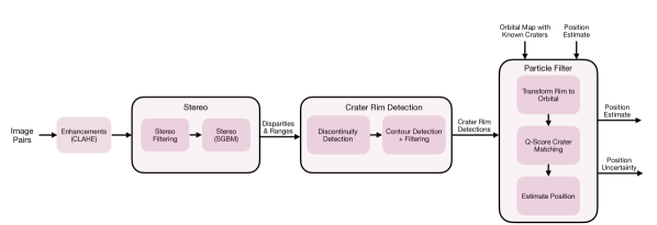
Figure 2: The four key components of the ShadowNav algorithmic pipeline are illustrated here. The system entails enhancing the image and then performing stereo and then a crater rim detection. This crater rim detection is then used as an input sample to a particle filter to perform absolute localization.

3.1 Image Enhancement

The first step in our system is to utilize Contrast Limited Adaptive Histogram Equalization (CLAHE) [Yadav et al., 2014] to enhance the raw images. In this work, we consider a single light source with consistent illumination provided across the field of light. Therefore, there is a significant decrease in pixel intensity values captured by a camera as the range increases of the physical region being imaged. Since CLAHE is adaptive, it equalizes the image within sub-regions, producing a more consistent image brightness to use as input to stereo algorithms. A potential downside of CLAHEs is that it can magnify noise within the image which is explored within this work.

3.2 Stereo

The second step within our system is to compute stereo. This is accomplished utilizing [Kogan,] and SGBMs [Hirschmuller, 2007]. The disparity and range maps produced provide the input for crater detection algorithms. In order to handle noisy disparity measurements in the far range, an additional cleanup step is used after stereo is computed.

Stereo Refinement: In order to perform stereo refinement, it is assumed that the terrain will be mostly planar with ranges increasing as the pixel indices get closer to the top row of the image. Therefore, to filter the far range noisy stereo measurements, the average range for all image rows are first computed. Next, these average row values are searched starting at ranges beyond a parameter, $20\text{\,}\mathrm{m}$, in this work. During this search, if the range decreases for a parameterized number of rows consistently, then all computed stereo values after this peak are removed.

3.3 Crater Leading Edge Detection

After stereo is computed, this output is utilized to perform crater leading edge detection. This is done with two components. The first is to detect discontinuities within the disparity and range images and the second is to connect these discontinuity locations into a single rim via a contour detection.

Discontinuity Detection: To perform the discontinuity detection, vertical columns within the disparity image are searched from bottom to top with holes removed from the search. Along the search if both a disparity discontinuity and range discontinuity are larger than set thresholds then the pixel at the start of the discontinuity is marked within a mask.

Contour Detection and Refinement: Once the discontinuity detection is complete, the detected mask image is dilated and then eroded to connect potentially noisy detections. Next, a contour detection algorithm is run over the mask to connect marked pixels. These contours are then filtered by both number of pixels and estimated length. The length of the contour is estimated by taking the average range value of all pixels in a contour and computing the width via Equation (1):

$$W_{m}=\frac{W_{px}*R_{m}}{l_{\textrm{focal}}},$$ (1)

where $W_{m}$ is the width of the crater rim in meters, $R_{m}$ the average range to each pixel in meters, and $l_{\textrm{focal}}$ if the focal length of the camera.

3.4 Absolute Localization via Particle Filter

Algorithm 1 Q-Score Computation

0:  Belief $b_{i}^{t}$, set of crater observations $\{z_{0,\textrm{rover}}^{t},\makebox[9.00002pt][c]{.\hfil.\hfil.}{},z_{m,\textrm{rover}}^{t}\}$, set of ground truth craters $\{c_{0,\textrm{world}}^{t},\makebox[9.00002pt][c]{.\hfil.\hfil.}{},c_{\ell,\textrm{world}}^{t}\}$, positive value $\varepsilon$ 

1:  $\mathcal{Q}_{\textrm{inc}}\leftarrow\varepsilon$ 

2:  for $i=1,\ldots,m$ do

3:   $z_{0,\textrm{world}}^{t}\leftarrow\textrm{rover\_to\_world}(z_{0,\textrm{rover}}^{t})$ 

4:   $d_{\textrm{cr}}\leftarrow\min\|c_{j,\textrm{world}}-z_{0,\textrm{world}}^{t}\|$ 

5:   ${\mathcal{Q}}_{\textrm{inc}}\leftarrow{\mathcal{Q}}_{\textrm{inc}}+d_{\textrm{cr}}$ 

6:  end for

7:  $Q_{\textrm{score}}\leftarrow\min\Big{(}1,(\frac{1}{m}{\mathcal{Q}}_{\textrm{inc}})^{-1}\Big{)}$ 

8:  return  $Q_{\textrm{score}}$

Algorithm 2 ShadowNav Particle Filtering Algorithm

0:  Initial belief distribution $(\mu_{0},\Sigma_{0})$, number of particles $N_{s}$, number of effective particles threshold $N_{\textrm{eff,thresh}}$ 

1:  $\{b_{1}^{0},\makebox[9.00002pt][c]{.\hfil.\hfil.}{},b_{N_{s}}^{0}\}\leftarrow\textrm{sample\_beliefs}(\mu_{0},\Sigma_{0})$ 

2:  $\{w_{1}^{0},\makebox[9.00002pt][c]{.\hfil.\hfil.}{},w_{N_{s}}^{0}\}\leftarrow\{1,\makebox[9.00002pt][c]{.\hfil.\hfil.}{},1\}$ 

3:  $t\leftarrow 1$

4:  while  particle filter running do

5:   $\{z_{0}^{t},\makebox[9.00002pt][c]{.\hfil.\hfil.}{},z_{m}^{t}\}\leftarrow\textrm{get\_observations()}$ 

6:   $\{q_{1}^{t},\makebox[9.00002pt][c]{.\hfil.\hfil.}{},q_{N_{s}}^{t}\}\leftarrow\{0,\makebox[9.00002pt][c]{.\hfil.\hfil.}{},0\}$ 

7:   for  $i=1,\makebox[9.00002pt][c]{.\hfil.\hfil.}{},N_{s}$  do

8:     $b_{i}^{t}\leftarrow\textrm{propagate\_sample}(b_{i}^{t-1})$ 

9:     $q_{i}^{t}\leftarrow\log\textrm{Q\_score}(b_{i}^{t},\{z_{0}^{t},\makebox[9.00002pt][c]{.\hfil.\hfil.}{},z_{m}^{t}\})$ 

10:   end for

11:   $q_{\textrm{min}}^{t}\leftarrow\min(q_{1}^{t},\makebox[9.00002pt][c]{.\hfil.\hfil.}{},q_{N_{s}}^{t})$ 

12:   for  $i=1,\makebox[9.00002pt][c]{.\hfil.\hfil.}{},N_{s}$  do

13:     $w_{i}^{t}\leftarrow w_{i}^{t-1}+q_{i}^{t}-q_{\textrm{min}}^{t}$ 

14:   end for

15:   $N_{\textrm{eff}}\leftarrow\textrm{compute\_N}_{\textrm{eff}}(w_{1}^{t},\makebox[9.00002pt][c]{.\hfil.\hfil.}{},w_{N_{s}}^{t})$ 

16:   if $N_{\textrm{eff}}\leq N_{\textrm{eff,thresh}}$ then

17:     $\{b_{1}^{t},\makebox[9.00002pt][c]{.\hfil.\hfil.}{},b_{N_{s}}^{t}\}\leftarrow\textrm{resample\_beliefs}(\{b_{i}^{t}\}_{i=1}^{N_{s}},\{w_{i}^{t}\}_{i=1}^{N_{s}})$ 

18:     $\{w_{1}^{t},\makebox[9.00002pt][c]{.\hfil.\hfil.}{},w_{N_{s}}^{t}\}\leftarrow\{1,\makebox[9.00002pt][c]{.\hfil.\hfil.}{},1\}$ 

19:   end if

20:   $t\leftarrow t+1$

21:  end while

Algorithm 3 Systematic Resampling

0:  Particles $\{b_{1}^{t},\makebox[9.00002pt][c]{.\hfil.\hfil.}{},b_{N_{s}}^{t}\}$ and associated weights $\{w_{1}^{t},\makebox[9.00002pt][c]{.\hfil.\hfil.}{},w_{N_{s}}^{t}\}$

1:  $n^{t}=\log\Big{(}\sum_{i=1}^{N_{s}}\exp(b_{i}^{t})\Big{)}$ 

2:  $\{\tilde{w}_{0}^{t},\makebox[9.00002pt][c]{.\hfil.\hfil.}{},\tilde{w}_{N_{s}}^{t}\}\leftarrow\{0,\makebox[9.00002pt][c]{.\hfil.\hfil.}{},0\}$ 

3:  for $i=1,\makebox[9.00002pt][c]{.\hfil.\hfil.}{},N_{s}$ do

4:   $\tilde{w}_{i}^{t}\leftarrow\exp(w_{i}^{t}-n^{t})$ 

5:  end for

6:  $\{q_{0},\makebox[9.00002pt][c]{.\hfil.\hfil.}{},q_{N_{s}}\}\leftarrow\textrm{cum\_sum}(\{\tilde{w}_{0}^{t},\makebox[9.00002pt][c]{.\hfil.\hfil.}{},\tilde{w}_{N_{s}}^{t}\})$ 

7:  $n\leftarrow 0$

8:  $m\leftarrow 0$

9:  $u_{0}\sim{\mathbb{U}}(0,\frac{1}{N_{s}})$ 

10:  while $n\leq N_{s}$ do

11:   $u=u_{0}+\frac{n}{N_{s}}$

12:   while $q_{m}\leq u$ do

13:     $m\leftarrow m+1$

14:   end while

15:   $n\leftarrow n+1$

16:   $b_{n}^{t}\leftarrow b_{m}^{t}$

17:  end while

18:  return  $\{b_{0}^{t},\makebox[9.00002pt][c]{.\hfil.\hfil.}{},b_{N_{s}}^{t}\}$

Here, we provide an overview of the proposed ShadowNav particle filtering approach. First, we provide further details on the Q-Score metric that is used in the belief update step.

3.5 Orbital Crater Ground Truth

In this work, we consider only specific ground truth craters which require a planned trajectory to drive towards. To this end, only the specific landmark craters to be used for global localization are labeled. When the estimated particle filter position was not within $20\text{\,}\mathrm{m}$ of the ground truth rim, the particle filter was not run and the position was propagated by a simulated noisy relative localization estimate update specified in Section 3.6. Secondly, only the front half of a crater is used as ground truth. However, since the landmark crater can be approached from any angle, the entire crater rim is labeled and the front half of the rim is determined dynamically based on the heading of camera at a specific time. Only the front edge of the crater is used as ground truth as our detection algorithm is only attempted to detect the front half and using the entire crater rim for matching could lead to false positives.

3.5.1 Q-Score

In each iteration of the particle filter, we compute what is known as the Q-Score, the probabilistic weight that some position belief corresponds to the true rover position. Algorithm 1 outlines the procedure for computing the Q-Score and the inputs necessary for the Q-Score computation are the belief $b_{i}^{t}$, a set of $m$ observed edges in rover frame, and a set of $\ell$ ground truth crater observations to associate these measurements with (Line  ‣ 1). The initial value $\mathcal{Q}_{\textrm{inc}}$ is set to some negligibly small, positive value $\varepsilon$ to later avoid divide-by-zero issues (Line 1) and is updated based on the distance between the observed edge and its associated ground truth observation (Line 4-5). The Q-Score is computed as the reciprocal of $\mathcal{Q}_{\textrm{inc}}$ and a $\min$ operation is applied to normalize the value between 0 and 1 (Line 7). We note that the $\min$ operation is applied based on the orbital DEM resolution in order to have the same Q-Score assigned for any observations and belief pairs that are less than or equal $1\text{\,}\mathrm{m}$ away from ground truth.

3.5.2 Filtering System

Algorithm 2 provides the full outline for the ShadowNav particle filtering algorithm. The algorithm takes as input a Gaussian belief distribution $(\mu_{0},\Sigma_{0})$ assumed for the initial robot position, the number of particles $N_{s}$ to use in the particle filter, and a threshold for the effective number of beliefs $N_{\textrm{eff,thresh}}$ used to trigger resampling (Line  ‣ 2). The filter is initialized with $N_{s}$ particles drawn from the initial belief distribution and each assigned equal weight (Lines 1-2). Given a new set of crater observations (Line 5), a set of Q-Score measurements is initialized for computing for each individual particle (Line 6). After applying the motion model update to each particle (Line 8), the Q-Score for each updated particle is computed using the procedure from Alg. 1 by comparing against the current measurements (Line 9). As is standard in many particle filtering implementations [Arulampalam et al., 2002], we note that the particle weights are updated in the in $\log$-domain (Line 13) with a normalization step to ensure non-negative weights (Line 11). Next, the number of effective samples $N_{\textrm{eff}}$ at the current iteration is calculated (Line 15). If $N_{\textrm{eff}}$ is below the threshold $N_{\textrm{eff,thresh}}$, then this is seen as an indication of particle filter “degeneracy”, wherein the weights $\{w_{i}^{t}\}$ collapse around a handful of particles. In such a case, a new set of particles are resampled using the systematic resampling scheme (Line 17).

Algorithm 3 provides an outline of the systematic resampling scheme used in this work. Given a set of particles and their associated weights, the weights are first normalized to $(0,1]$ from $\log$-domain (Lines 1-4) and the cumulative sum of these normalized weights $\tilde{w}_{i}^{t}$ computed (Line 6). The systematic resampling procedure then samples a random value $u_{0}$ from a uniform distribution inversely proportional to $N_{s}$ (Line 9) and this ensures that at least one particle is retained from each $\frac{1}{N_{s}}$ interval from the previous belief distribution.

3.6 Simulating Relative Localization

In order to simulate the impact of drift from relative localization, a bias factor is added. This is in addition to the Gaussian noise factor used in our previous work. This bias is a Gaussian distributed magnitude with the mean as the specified percentage drive of relative localization and a constant unit vector direction. The unit vector direction is randomly chose from a uniform distribution of all possible directions at the start of a replay of a trajectory. For example if the relative localization error rate used is 2% then at each step, the bias factor is a Gaussian centered around 2% of the distance traversed in that step. Over the course of many Monte Carlo runs, the bias will be added in many different directions to test for drift in all directions.

4 Data Collection

In this section, we present details on the datasets generated to validate the efficacy of the proposed ShadowNav approach. We first review the simulation environment used to generated photorealistic stereo data and then review the configuration used to collect nighttime field testing data from the Cinder Lakes, Arizona.

4.1 Simulation

In this work, we develop a simulation environment using the Blender software, which has become a popular software framework for generating photorealistic images in a Lunar environment[Crues et al., 2023, Cauligi et al., 2023]. Within this simulation, the Hapke lighting model [Hapke, 2002, Hapke, 2012, Schmidt and Bourguignon, 2019] was implemented which approximates the Lunar surface reflectance. This model will simulate the “opposition effect” which leads to a focused point of extreme saturation at a location within an image where the camera ray and light source are at zero phase angle. We implemented the Hapke lighting model using “old highland” parameters of the Moon provided in [Xu et al., 2020]. For our use case, the coherent backscattering opposition effect (CBOE) was left out of our implementation and only the shadow hiding opposition effect (SHOE) was implemented as it dominates most or all lighting calculations.

To obtain a realistic 3D model of the surface geometry, DEMs produced from LROC were utilized.  LROC resolution is typically between $2\text{\,}\mathrm{m}$-$5\text{\,}\mathrm{m}$ which allows for resolving craters of approximately $10\text{\,}\mathrm{m}$. However, as the LROC resolution is insufficient for generating smooth surface imagery, the DEMs from LROC were scaled down to be $0.25\text{\,}\mathrm{m}$ resolution. Crater measurements for simulated data in future discussions were based on this scaled resolution. This scaled DEM was imported into Blender and a surface texture comprised of two scales of fractal Brownian motion. This texture is a natural noise and simulates surface texture features for stereo algorithms to utilize.

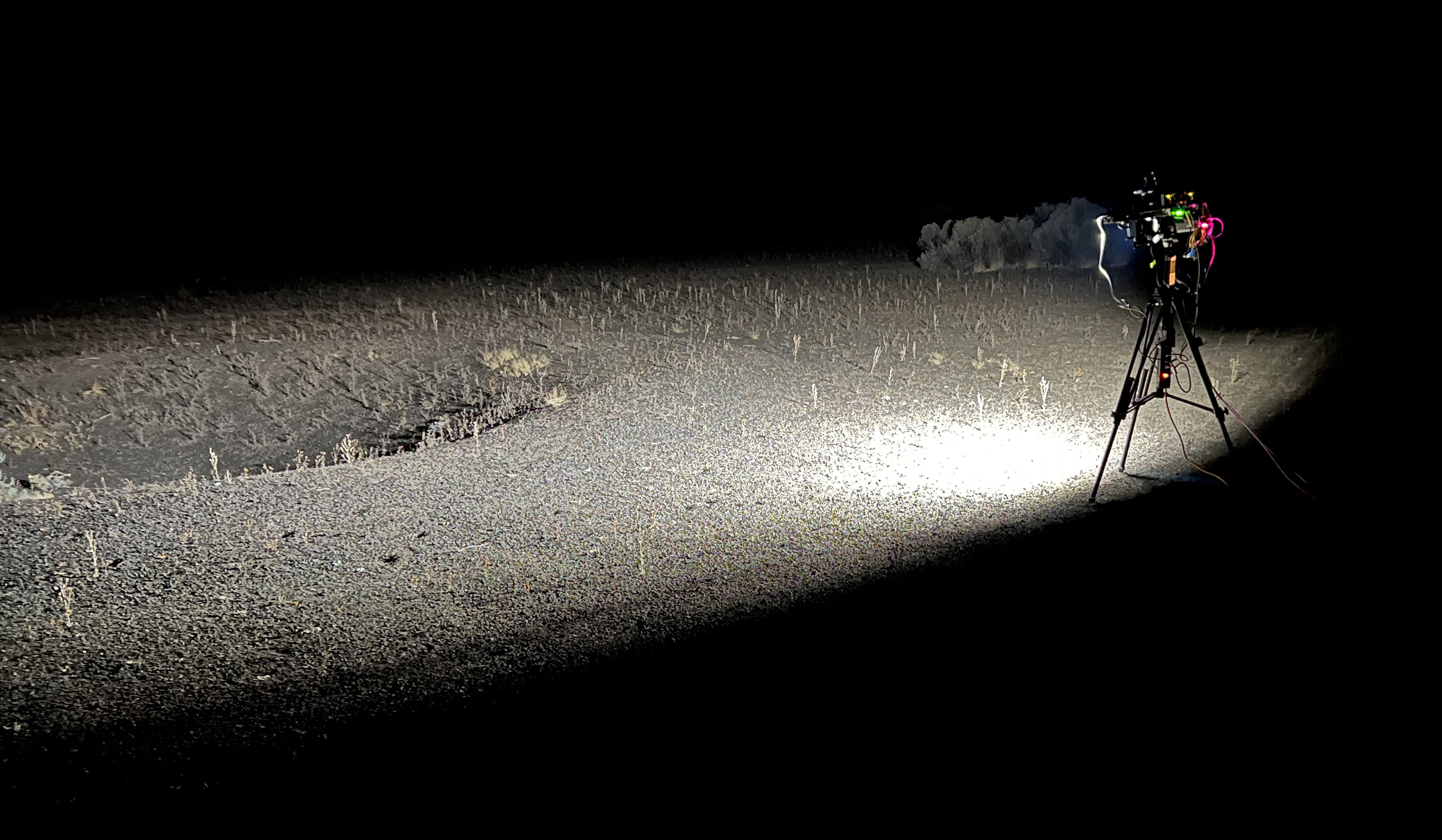
Figure 3: Image of the data collection rig capturing an image of a crater at Cinder Lakes Apollo Training Area.

4.1.1 Simulated Dataset

For simulation, we developed two datasets - one with the aim of testing the efficacy of our crater matching algorithm and a second dataset for testing the overall global localization pipeline. The crater matching dataset was created by selecting four craters from the orbital data of diameters between $5\text{\,}\mathrm{m}$ and $20\text{\,}\mathrm{m}$. The simulator was run to generate stereo pairs every $1\text{\,}\mathrm{m}$ at four angles around the crater (0^∘, 90^∘, 180^∘, and 270^∘) and at ranges between $5\text{\,}\mathrm{m}$-$25\text{\,}\mathrm{m}$. Additional datasets were created to test sensitivity to the parameters of the hardware configuration:

• Camera heights of $1.5\text{\,}\mathrm{m}$, $2.5\text{\,}\mathrm{m}$, and $3\text{\,}\mathrm{m}$ off the ground

• Light offsets of $0.2\text{\,}\mathrm{m}$ below the camera, inline with the camera and $0.2\text{\,}\mathrm{m}$ above the camera.

• Light power ranging from low, medium and high.

The second dataset generated was for localization across three different locations in the South Pole region of the Moon. Additionally at each location, three different types of trajectories were generated:

• a straight line trajectory

• a half survey where 180 degrees of the ground truth crater is observed

• a full survey where 360 degrees of the ground truth crater is observed

These trajectories ranged in length from $536\text{\,}\mathrm{m}$ to $840\text{\,}\mathrm{m}$ and contained two ground truth crater landmarks. An additional trajectory was created in a different region where the trajectory path in one direction was $1058\text{\,}\mathrm{m}$ and its reverse $1211\text{\,}\mathrm{m}$. The trajectory contained three ground truth crater landmarks and a top down view of this ground truth trajectory is in Figure 4.

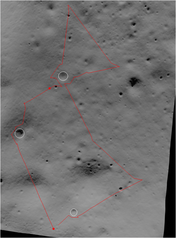
Figure 4: A $1000\text{\,}\mathrm{m}$+ simulated trajectory overlaid onto a simulated orbital map of the Lunar South Pole Region. The map contains ground truth landmark craters marked with white circles.

4.2 Cinder Lakes Apollo Training Area

We collected datasets from Cinder Lakes near Flagstaff, Arizona. This field test site was chosen as a Lunar analogue site as a realistic crater distribution of appropriate crater sizes was constructed during the Apollo era at two different sites:

1. The south site is $500\text{\,}\mathrm{ft}$-by-$500\text{\,}\mathrm{ft}$ in area and is well preserved as it is protected from motorized vehicles, but it does have areas of vegetation growth.

2. The north site is 1200’-by-1200’ and has almost no vegetation, but it is more heavily eroded due to being within an off-highway vehicle area.

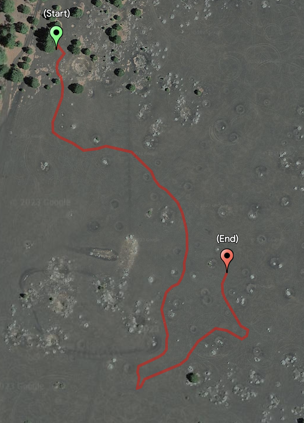
(a)

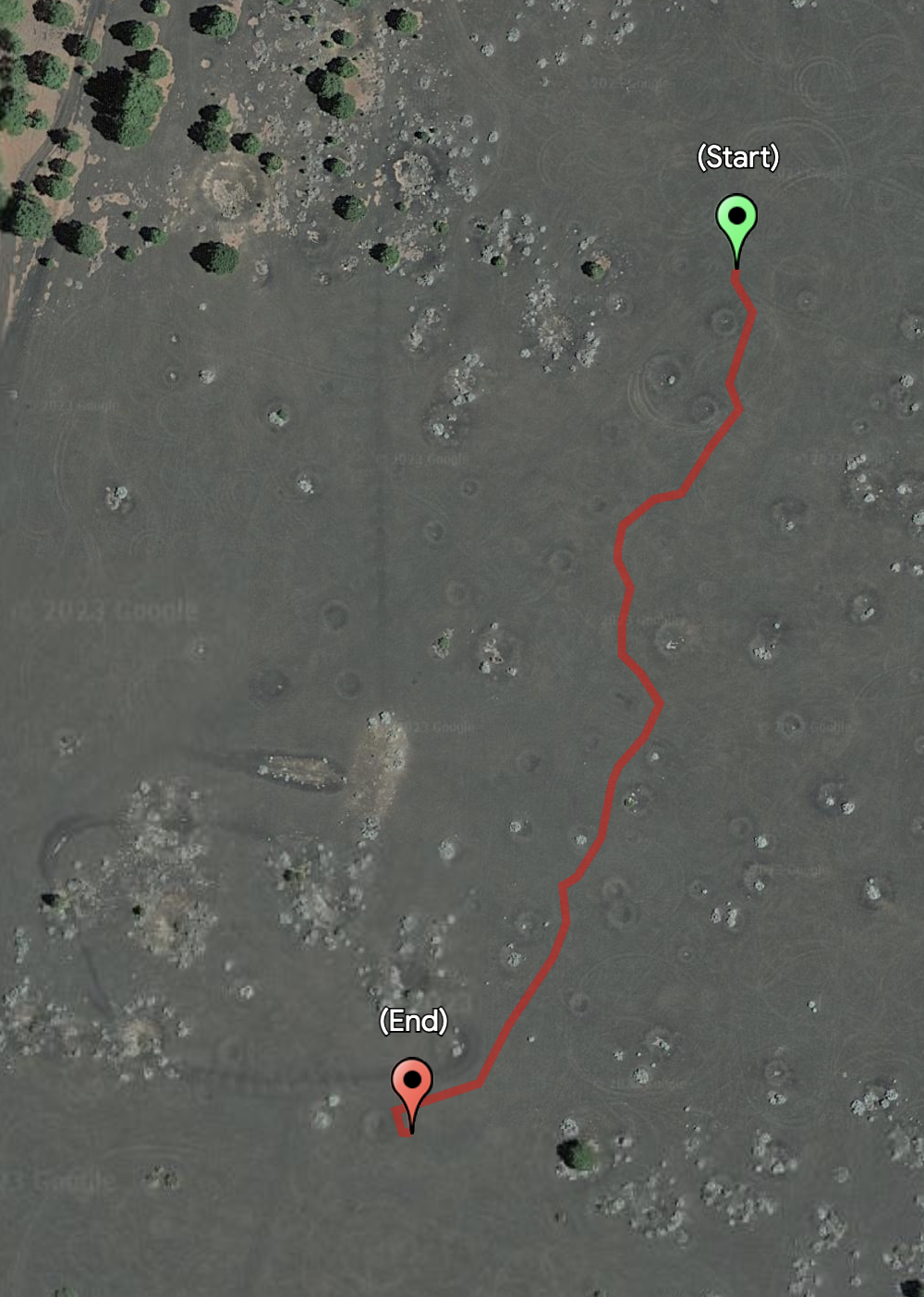
(b)

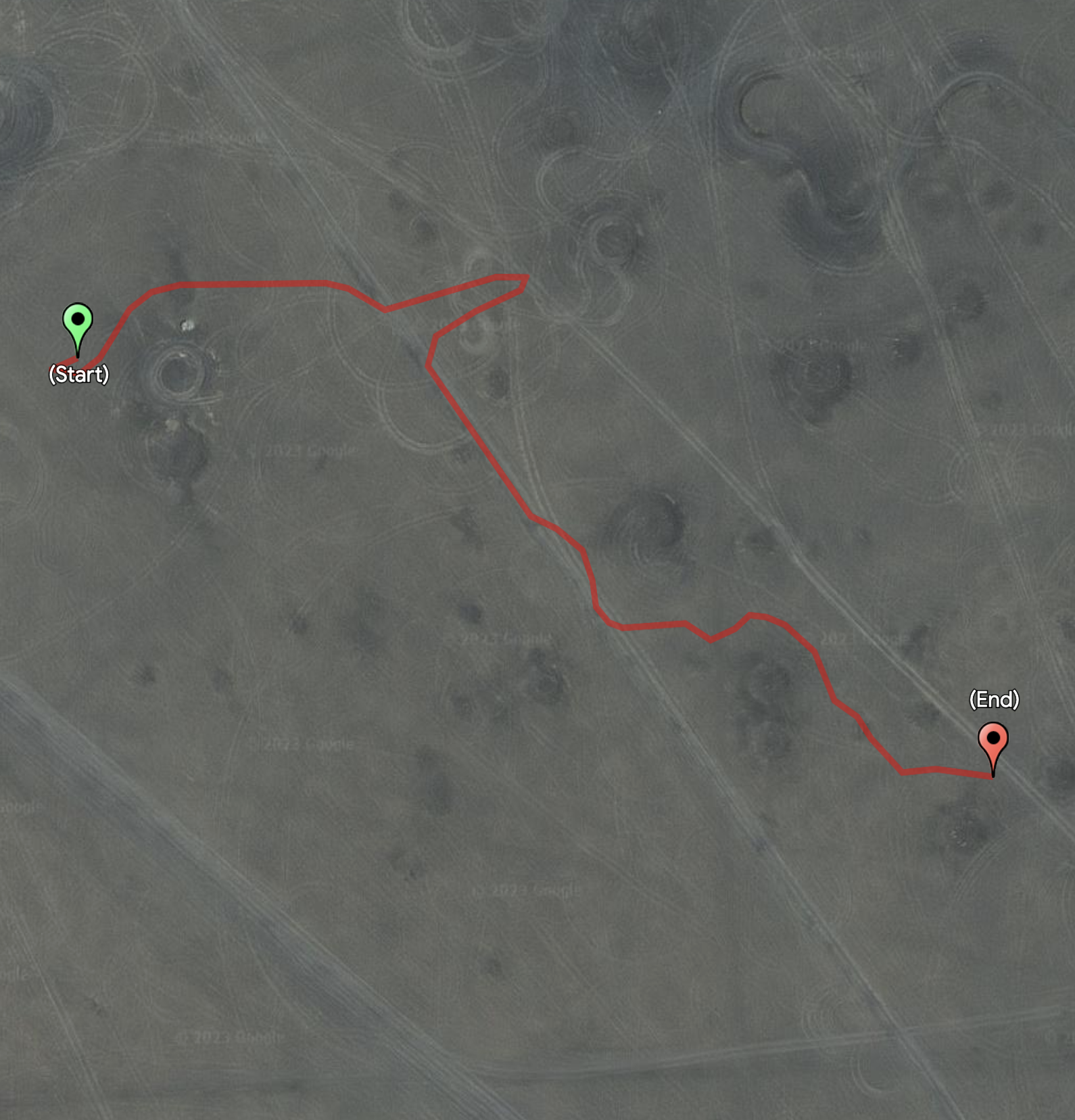
(c)

Figure 5: Three trajectories collected in the Cinder Lakes Apollo training area. (a) and (b) were collected in the better preserved South site and (c) was collected in the North site which is part of an OHV Area.

Our datasets were collected during a New Moon and, given that Cinder Lakes is located outside of the dark sky town of Flagstaff, Arizona, the conditions allowed for an environment with minimal ambient light similar to what would be encountered in dark Lunar environments. In order to perform the data collection, we used a data collection rig consisting of a stereo camera with a $0.26\text{\,}\mathrm{m}$ baseline, 5,120-by-3,840 pixel resolution, and 60^∘ horizontal field-of-view as shown in Figure 3. Additionally a $50\text{\,}\mathrm{W}$, $5000\text{\,}\mathrm{lm}$ flood light was placed below the camera, with the light area ranging from $0.1\text{\,}\mathrm{m}$-$0.2\text{\,}\mathrm{cm}$ below the stereo cameras. There was a GPS inertial navigation system attached to the stereo cameras to provide ground truth position and orientation.

For the data collection, we performed two types of collections. The first type was geared toward perception tests. This involved moving the data collection rig from approximately $20\text{\,}\mathrm{m}$ away to $5\text{\,}\mathrm{m}$ from the leading crater edge with stops for long exposures roughly every $1\text{\,}\mathrm{m}$. The second type was geared toward localization tests. This entailed moving the data collection rig through the crater field with stops for long exposure approximately every $5\text{\,}\mathrm{m}$-$10\text{\,}\mathrm{m}$. During these stops the rig was directed toward large craters if any were present. In total, in this work, 12 craters ranging from $5\text{\,}\mathrm{m}$-$25\text{\,}\mathrm{m}$ in diameter and three trajectories were collected and used. The three different trajectories are displayed in Figure 5 which shows the GPS path within Google Earth satellite imagery. Of these, two trajectories were captured in the south site and one in the north site. In order to evaluate longer distances between craters, some experiments added drift error as if more distance had been traveled by artificially adding trajectory locations outside of the crater field at the start of a trajectory.

5 Results

In this section we detail the results of stereo, crater detection and matching, and absolute localization performance of our system.

5.1 Stereo

Table 1: Stereo performance evaluation using 4 different simulated crater samples across different parameters. “Height” is camera height above ground and “Offset” is the light offset relative to cameras. All metrics utilize range output from stereo. %hole is percentage of pixels that are holes where there is ground truth. %err is the percentage that have a range estimate greater than a threshold. RMS is the root-mean-square error in meters of reported range values.

0-10m Range 10-20m Range 20-30m Range 30-40m Range Height Offset Light %err RMS %err RMS %err RMS %err RMS Algo. (m) (m) Power %hole $>$0.5m (m) %hole $>$1m (m) %hole $>$2m (m) %hole $>$3m (m) SGBM 2.5 -0.2 high 6.82 1.27 0.28 11.94 18.06 1.02 34.67 20.85 1.47 82.84 8.90 1.47 SGBM 2.5 -0.2 med 3.68 1.07 0.28 11.76 15.34 0.77 38.64 20.30 1.37 85.22 14.93 1.74 SGBM 2.5 -0.2 low 4.04 0.96 0.28 23.99 16.79 0.64 73.98 25.77 1.57 98.05 45.26 3.75 SGBM 2.5 0.0 med 11.38 2.54 0.36 31.60 18.60 0.98 55.52 18.08 1.29 89.84 11.48 1.51 SGBM 2.5 0.2 med 74.13 16.50 1.34 60.97 25.64 1.45 69.53 17.81 1.28 93.26 11.96 1.53 SGBM 1.5 -0.2 med 6.71 1.58 0.22 27.53 24.94 1.15 50.30 21.78 1.48 88.38 21.51 2.34

In order to be able to effectively detect and match crater rims, accurate stereo is required. For detection, outliers in range values or stereo holes could lead to crater rim false positives. Furthermore, inaccurate stereo ranges could lead to poor projections into the orbital map which could cause good image-space detections to match poorly to orbital landmark craters. In order to evaluate stereo performance, we created a simulated dataset of craters with ground truth ranges which was detailed in Section 4.1.

To evaluate stereo performance, three metrics based on [Scharstein et al., 2001] binned across ground truth range values are used. These metrics are:

1. The percent of pixels with a stereo hole where the corresponding ground truth pixel has a value within a specified range.

2. The percent detected pixels where a corresponding ground truth pixel has a value within a specified range that is not a hole but has a detected range whose error relative to ground truth value is greater than a threshold.

3. The “root-mean-squared”s (RMSs) range error for all detected pixels that are not a hole and have a corresponding ground truth pixel within a specified range.

We note that a crucial difference between the metrics used in [Scharstein et al., 2001] is that range is used rather than disparity as range is what ultimately has the impact on crater matching and we have perfect camera calibrations within simulation.

To validate the impact of hardware system parameters such as light location, camera height, and light power, these parameters were swept and stereo performance evaluated. Light power is used as a proxy for exposure time and light brightness as these are not modelled well in Blender. High light power corresponds to the near range of the image being fully exposed (pixel value of 255). In order to provide additional realism for nighttime imagery, a zero-mean 1.2 pixel intensity sigma Gaussian noise was added to all images and the results of this analysis are in Table 1. In these results, we observe that the optimal configuration for stereo is with a $2.5\text{\,}\mathrm{m}$ camera off ground, light offset $0.2\text{\,}\mathrm{m}$ below the camera, and high light power. Medium light power at a camera height of $2.5\text{\,}\mathrm{m}$, wherein the near range is bright but few of the pixes are fully exposed, demonstrates improved performance but at the slight cost of degraded perofrmance at range. Moreover, although this configuration has robustness to camera height ranges, we observe that a camera height of $1.5\text{\,}\mathrm{m}$ performs slightly worse than other heights and this is attributed to cameras closer to the ground losing vertical resolution with range. Finally, a key takeaway is that placing the camera inline with the camera significantly degrades performance and placing the light above the camera renders performance extremely poor. We found that placing the light below the camera minimizes some of the opposition effect’s impacts and provides some shadowing on the surface for more visible features.

5.2 Crater Detection and Matching

In order to evaluate crater detection and matching, we utilized real data collected at Cinder Lakes as detailed in Section 4.2. Additional simulated data was collected to evaluate stereo and positional errors as detailed in Secion 4.1. In order to evaluate detection performance we utilize a metric that is percent of the ground truth front rim detected:

$$\%_{\textrm{rim}_{\textrm{det}}}=\frac{px_{\textrm{gt}_{\textrm{matched}}}}{px_{\textrm{gt}}}*100$$ (2)

,where $px_{\textrm{gt}_{\textrm{matched}}}$ is the number of ground truth crater points in world frame that have a detection that is closest to that ground truth point and $px_{\textrm{gt}}$ is the total number of all ground truth points. This detection does not consider false positives. In order to evaluate crater matching performance, we utilize the Q-Score metric detailed in Section 3.5.1 to evaluate how closely a perception sample aligns to orbital ground truth considering both matches and false positives.

SGBM stereo and discontinuity detection were run across the Cinder Lakes crater dataset to evaluate crater detection and matching performance. Figure 6 shows the results with respect to percent of front rim detected and Q-scores versus range and crater diameter are shown. From these results, we observed that nearly all craters have some level of detection between $5\text{\,}\mathrm{m}$-$15\text{\,}\mathrm{m}$. However, at $15\text{\,}\mathrm{m}$ the $7\text{\,}\mathrm{m}$-crater is no longer detected. Furthermore, the $25\text{\,}\mathrm{m}$ has worse results across most of the set of camera distances from the crater rim. The reduction in performance for smaller and larger craters is expected with our current approach. Since a discontinuity within stereo must be observed and not just an end to stereo detections, a larger crater diameter requires stereo to obtain matches at farther ranges to observe features on the far side. Additionally smaller diameter craters discontinuity gaps are more likely to decrease below threshold levels at increased range. Overall, we observe robust filter performance, with most samples containing a Q-Score of 0.4 or better which means that the average pixel detection is within $2\text{\,}\mathrm{m}$ of the crater rim and indicates low false positives and high accuracy.

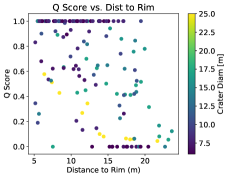
(a)

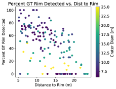
(b)

Figure 6: Cinder Lakes crater detection and matching results using SGBM and discontinuity detection. (a) Q-Scores. (b) Percent front arc of ground truth crater detected.

In order to further evaluate crater detection, simulated data is evaluated first by comparing crater rim detection and matching with and without Gaussian noise added. Figure 7 contains the results of comparing noise free versus images with zero mean, 1.2 sigma pixel intensity Gaussian noise added. From these results, it is observed that the addition of noise has minimal impact on crater detection performance. Compared with the Cinder Lakes results, however, detection performance is a bit worse at both close to $5\text{\,}\mathrm{m}$ to the crater and beyond $15\text{\,}\mathrm{m}$ from crater rim. The largest difference is in the Q-Score computation with similar crater rim detection performance to Cinder Lakes data. Potential sources of this performance difference include the simulation containing images with a wider field-of-view, a $2.5\text{\,}\mathrm{m}$ camera height compared to $1.5\text{\,}\mathrm{m}$ camera height for Cinder Lakes data, and the inherent simulation versus real differences in lighting, camera exposure handling, and surface textures.

The higher camera height would potentially allow the images to capture the near side of the crater and therefore limit the discontinuity. The larger field-of-view also would allow for more potential false positives to be captured as evidenced by strong crater rim percent detection but degraded Q-Scores at $15\text{\,}\mathrm{m}$-$20\text{\,}\mathrm{m}$ ranges to crater rims.

Figure 8 shows qualitative samples of both Cinder Lakes and simulated data images, stereo, and detections at $12\text{\,}\mathrm{m}$ from crater rims. We see from these samples that the simulated images have noisier stereo. Further, there are holes in the stereo images and especially at ranges greater than $15\text{\,}\mathrm{m}$. Such stereo holes could lead to false positives and Such stereo holes could lead to false positives and noisy stereo could potentially yield noisier edge detections. Finally, both Cinder Lakes and simulated imagery results in high-quality rim detections.

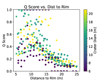
(a)

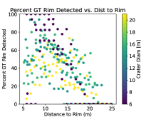
(b)

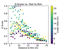
(c)

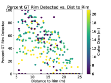
(d)

Figure 7: Crater detection and matching results with an without Gaussian noise added to simulated images on data with a camera height of 2.5m a light offset of 20cm below camera and high exposure. For images with noise added, 0 mean and 1.2 pixel intensity sigma were used. (a) Q score no noise (b) Percent detected no noise (c) Q Score 1.2 sigma noise (d) Percent detected 1.2 sigma noise.

(a)

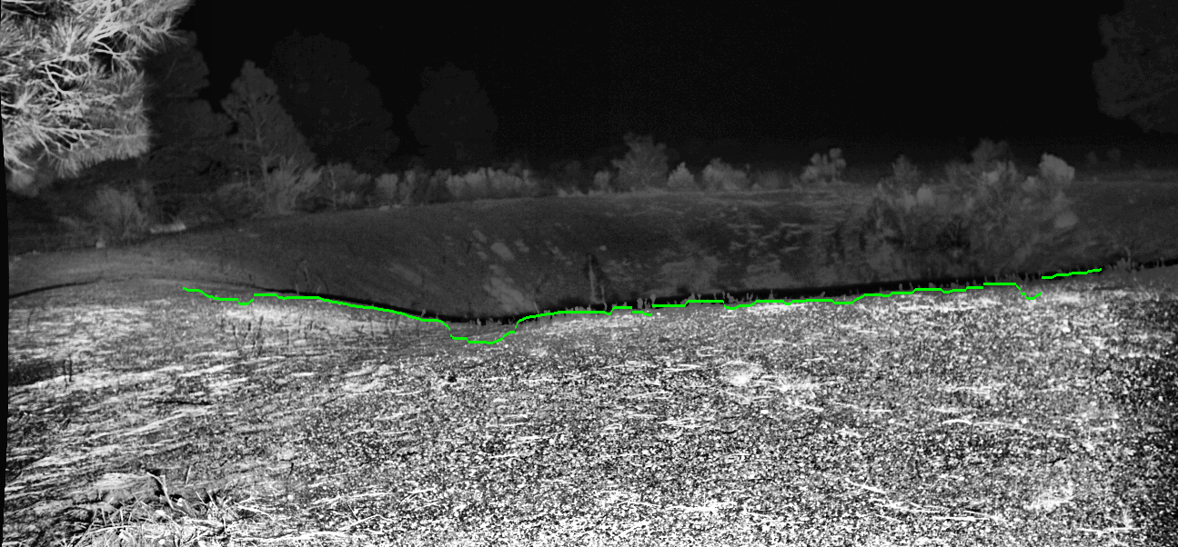
(b)

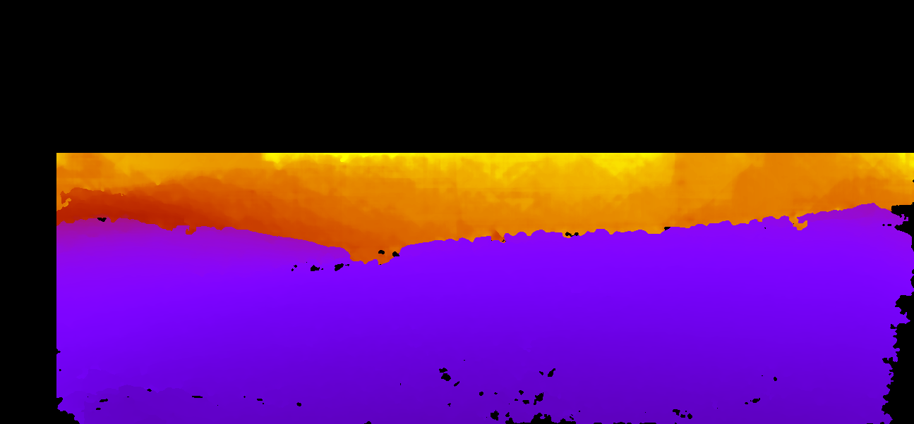
(c)

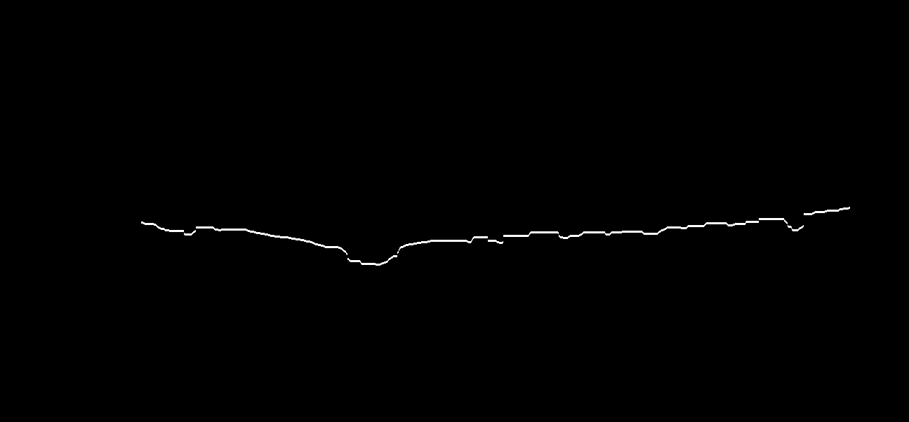
(d)

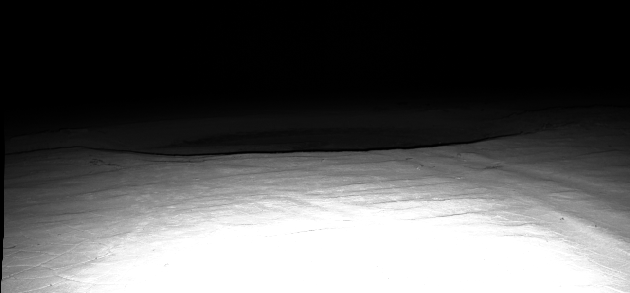
(e)

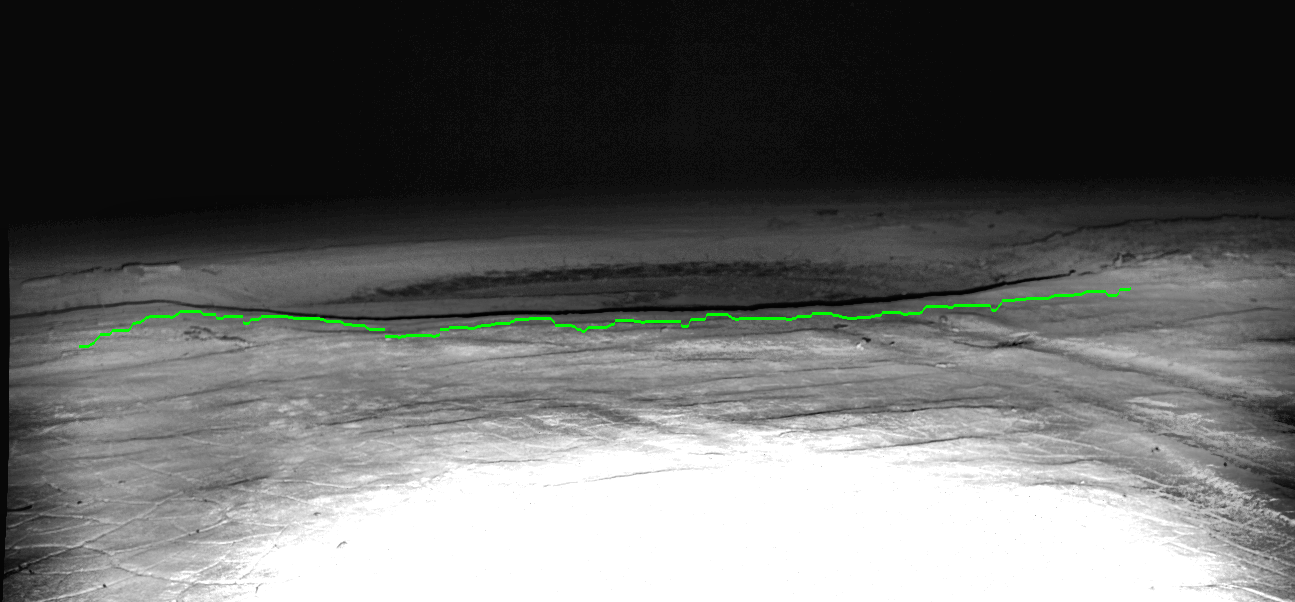
(f)

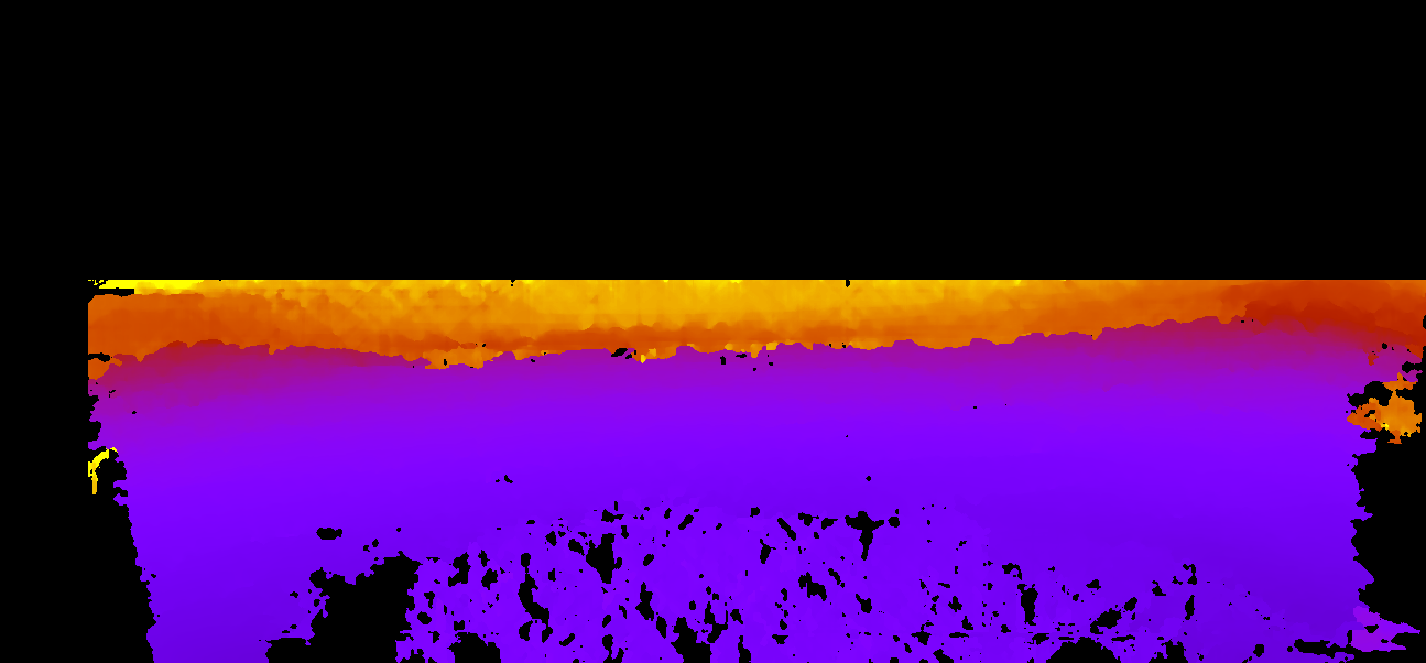
(g)

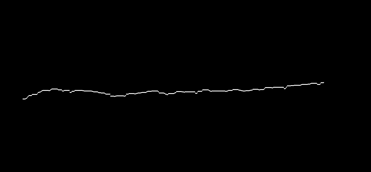
(h)

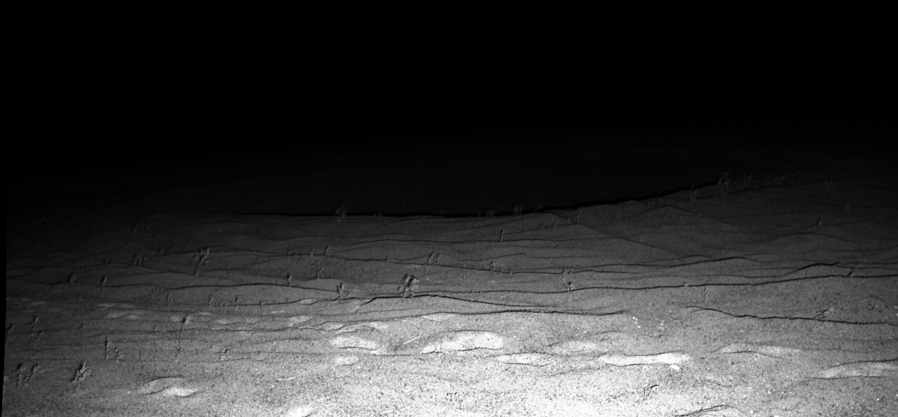
(i)

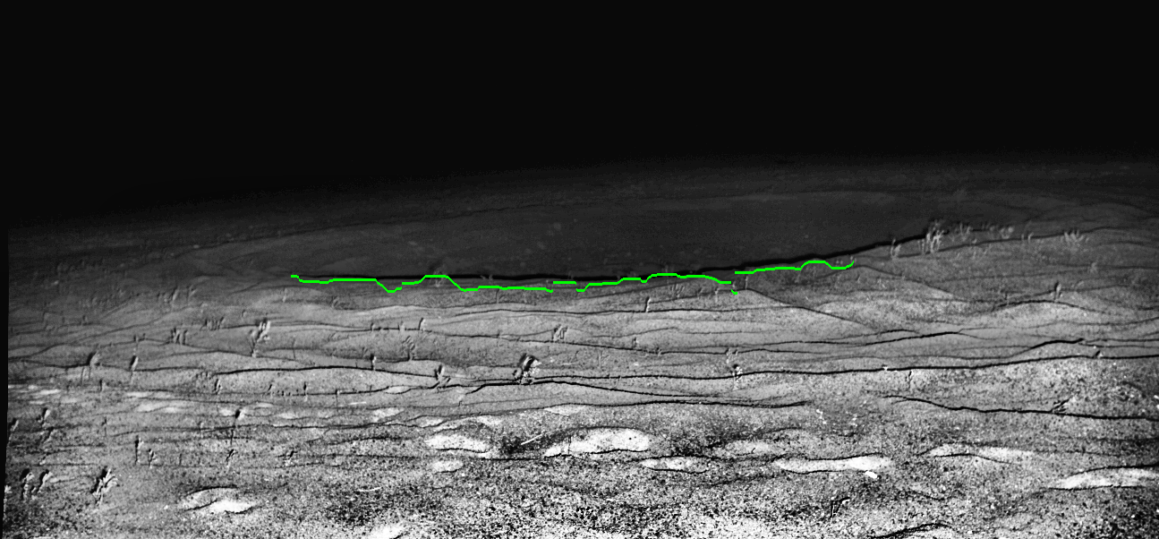
(j)

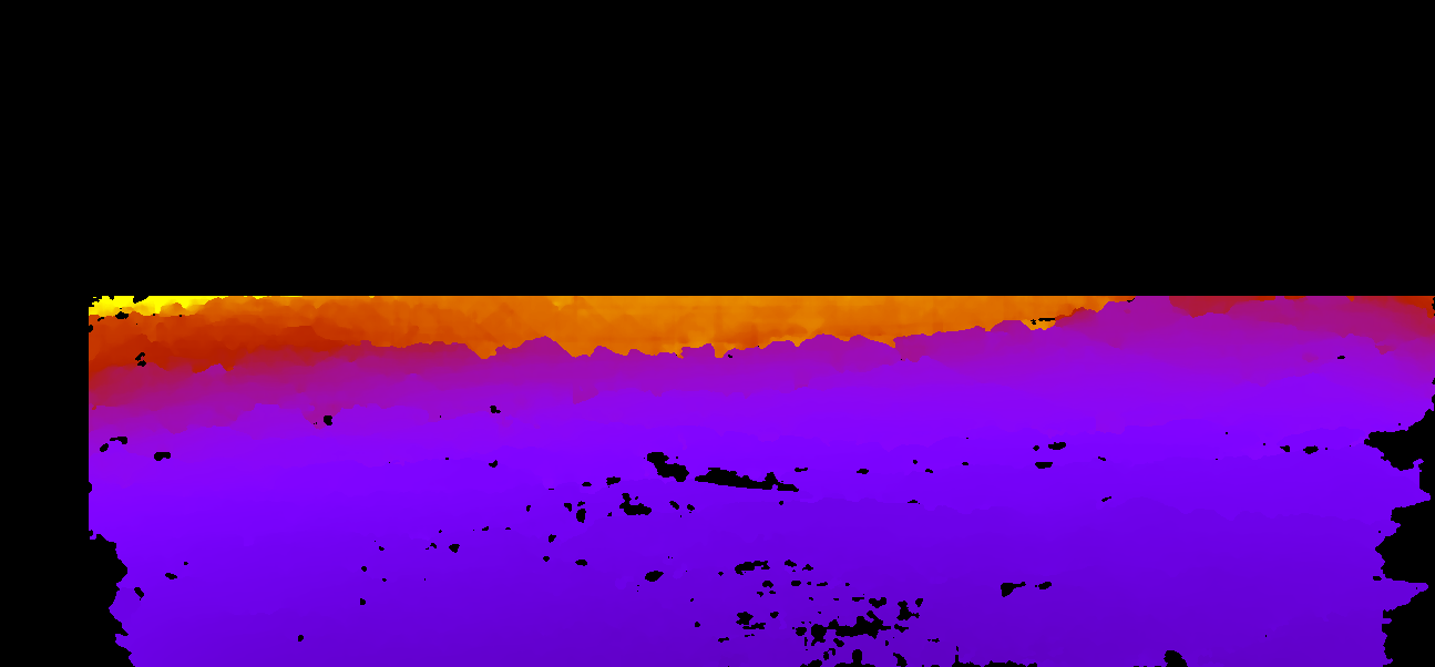
(k)

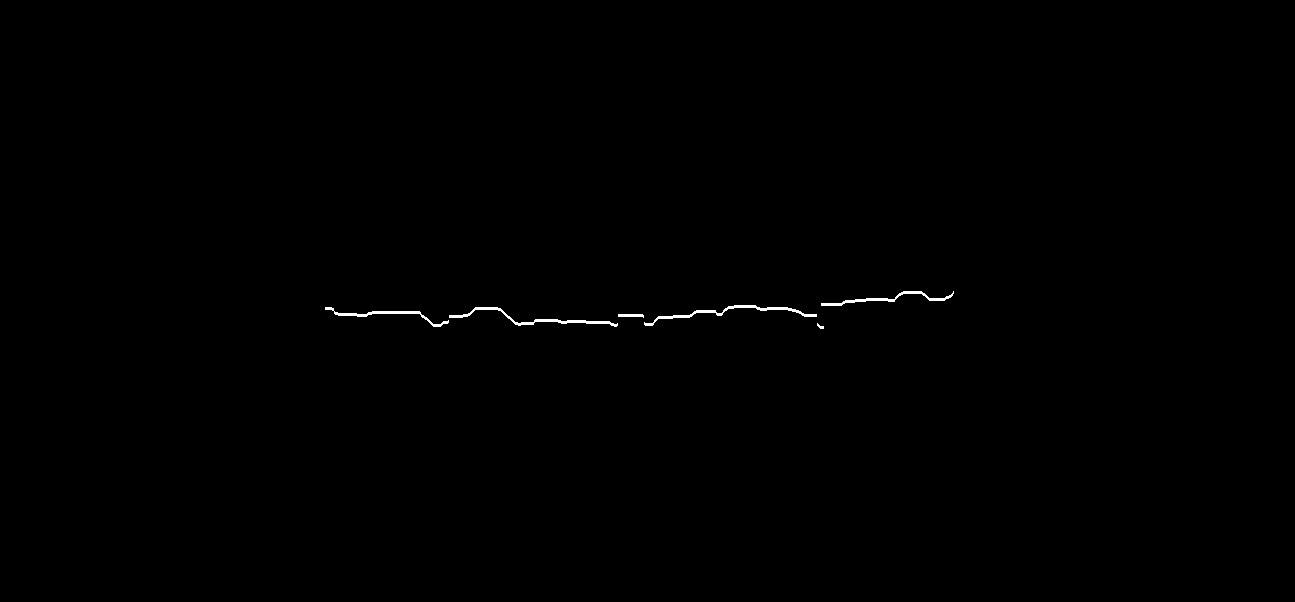
(l)

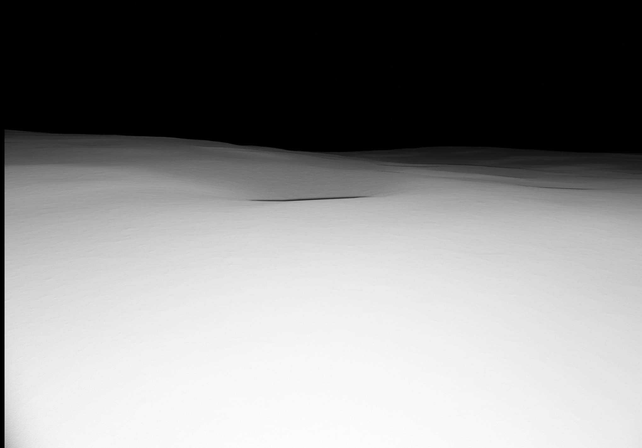
(m)

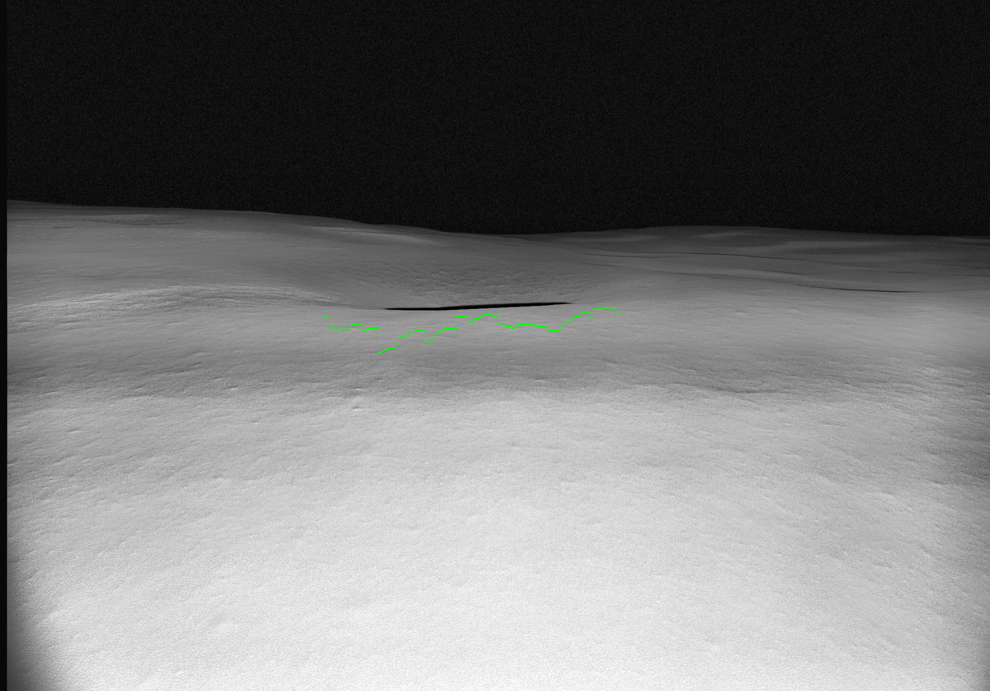
(n)

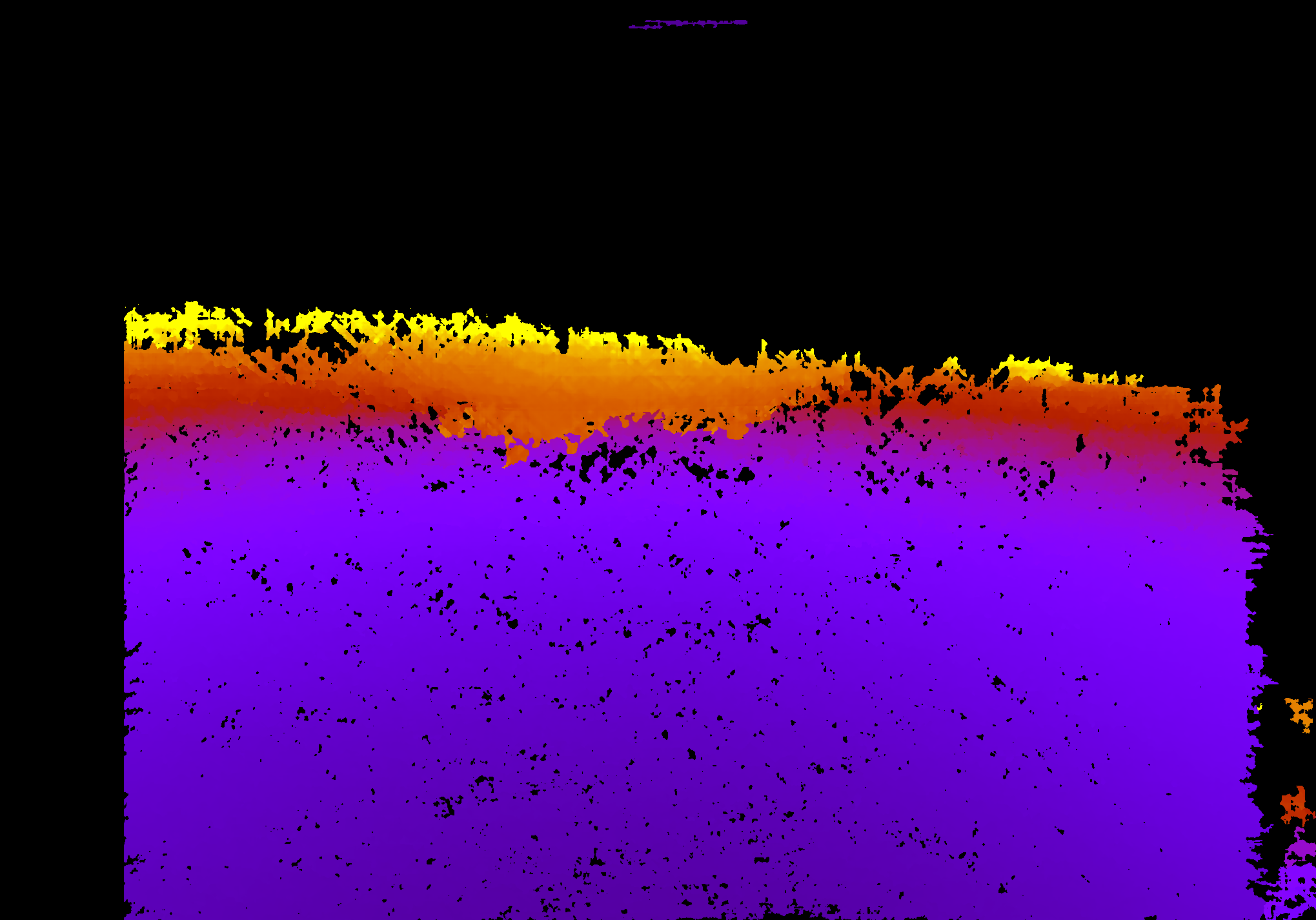
(o)

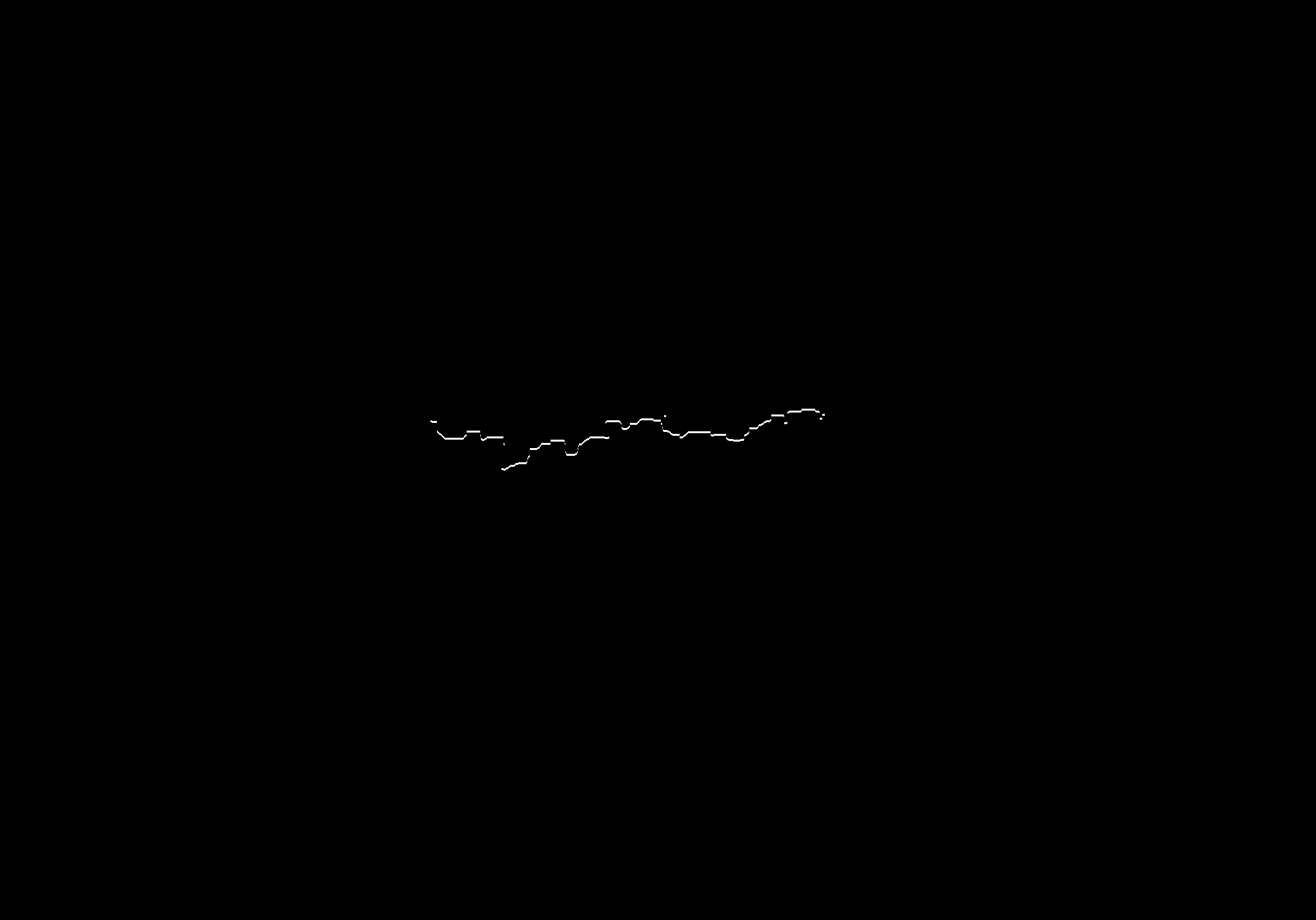
(p)

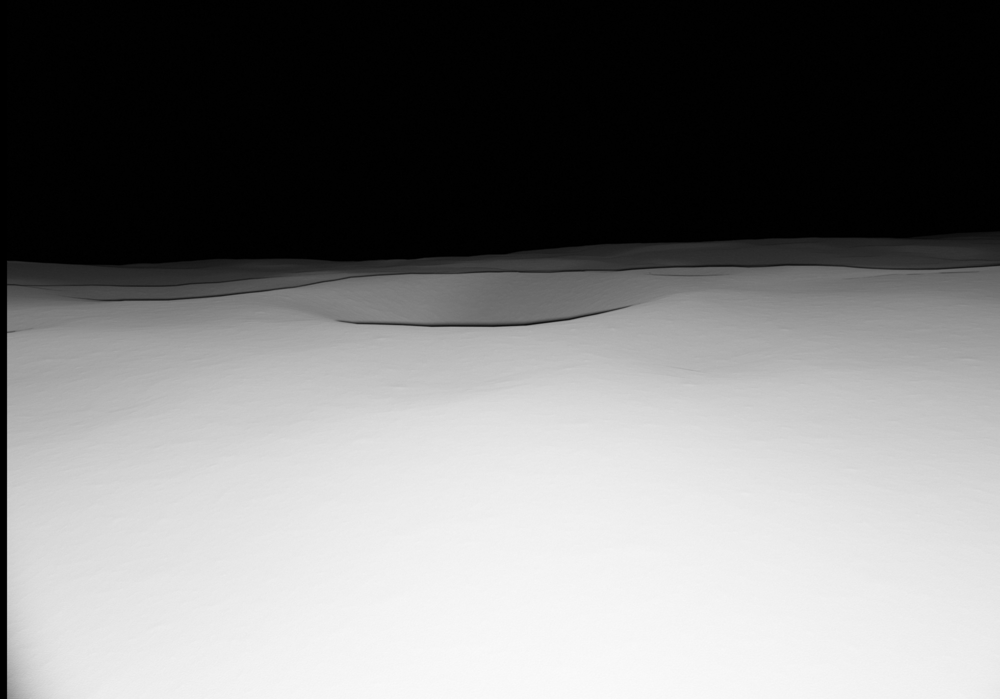
(q)

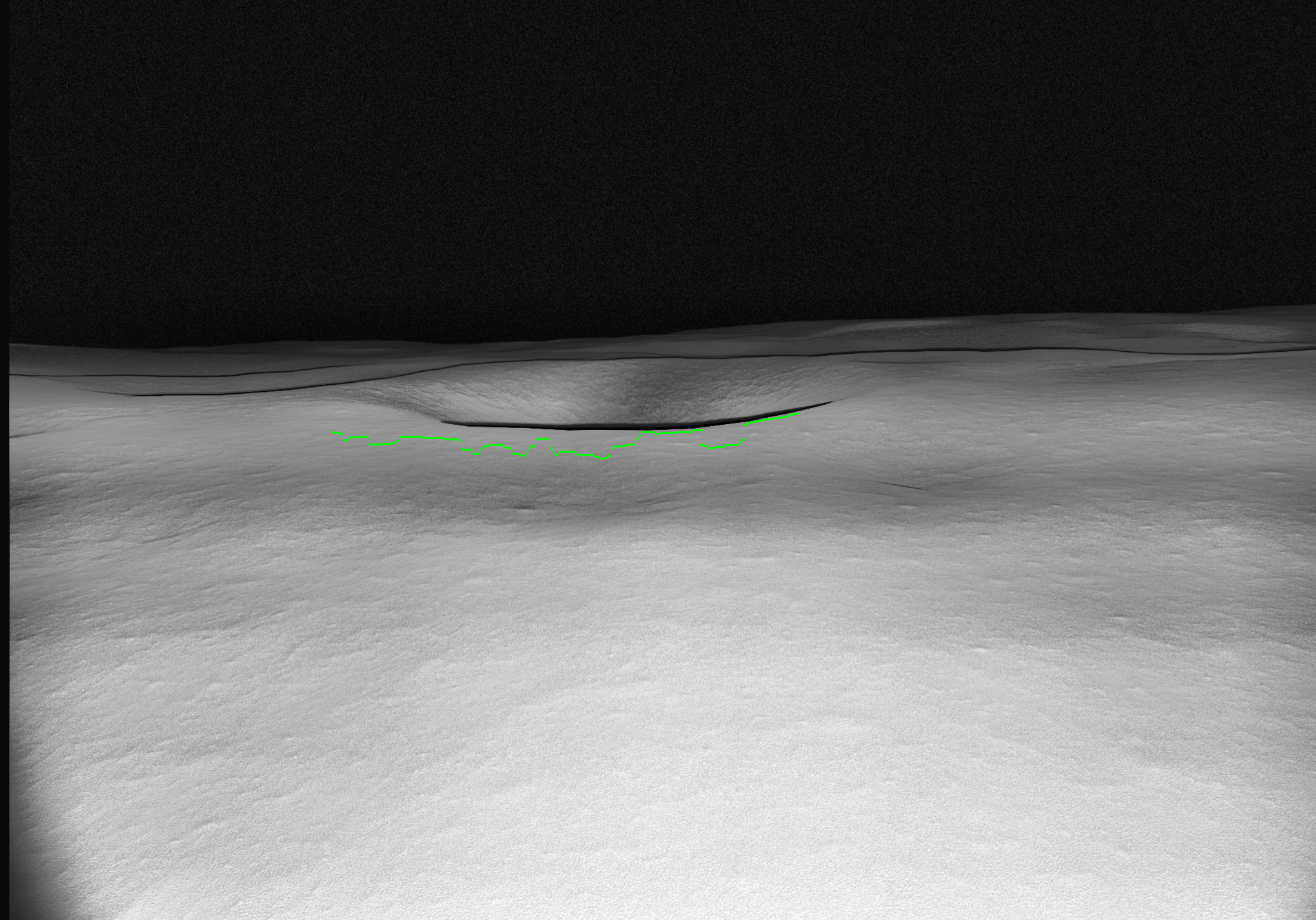
(r)

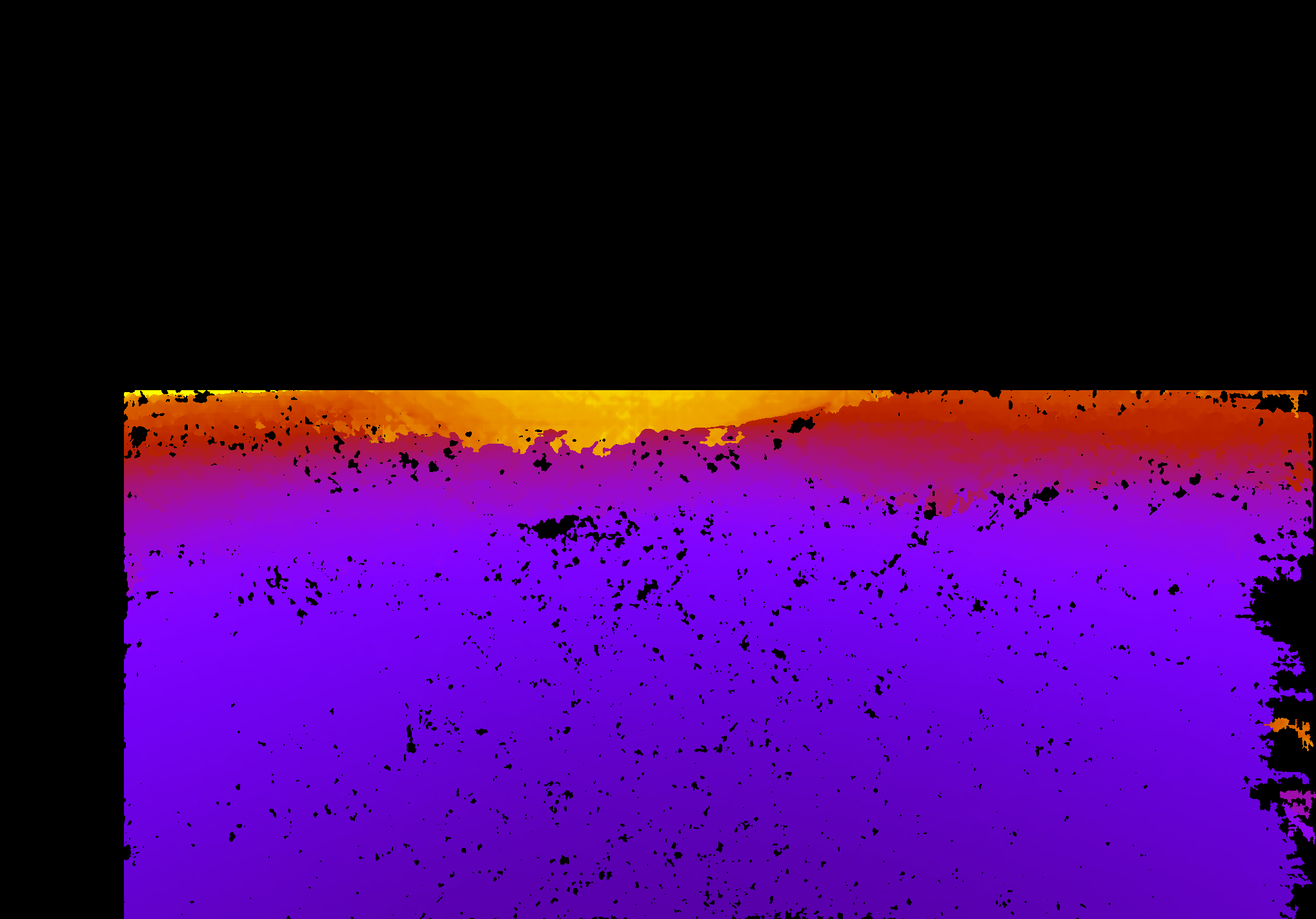
(s)

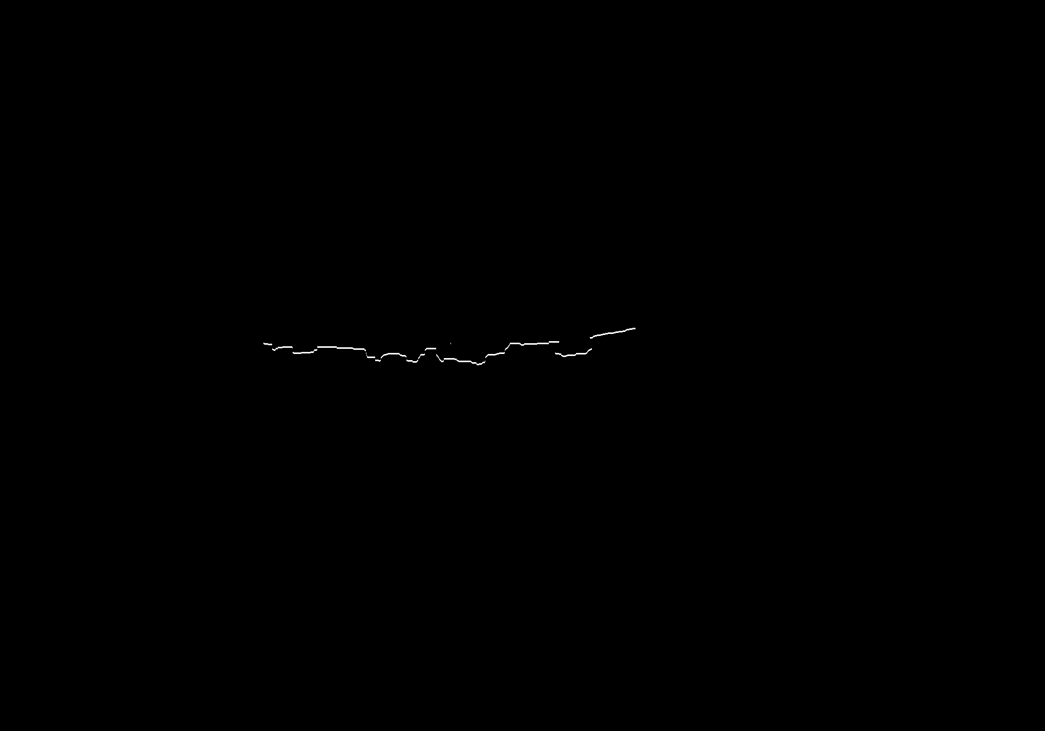
(t)

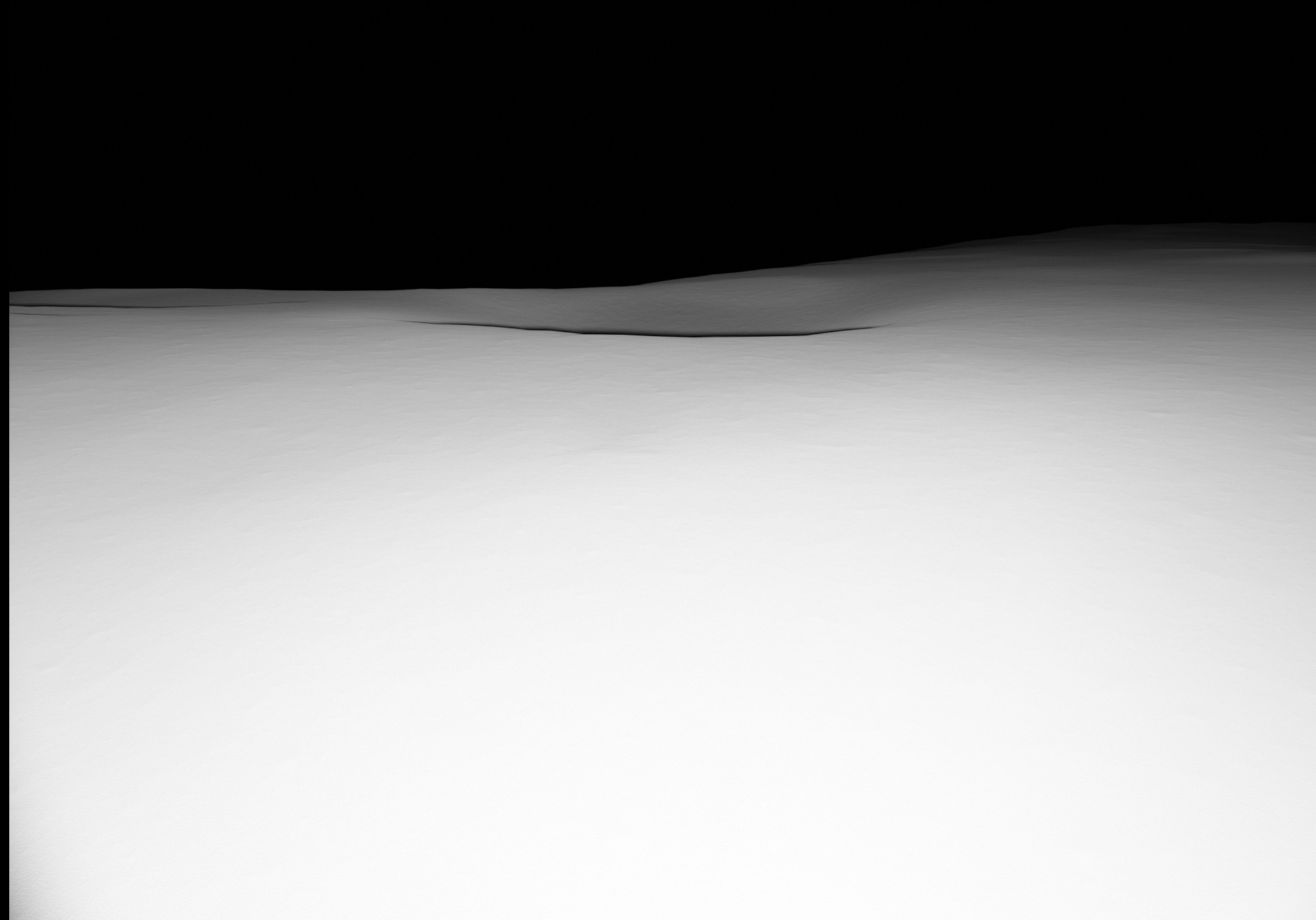
(u)

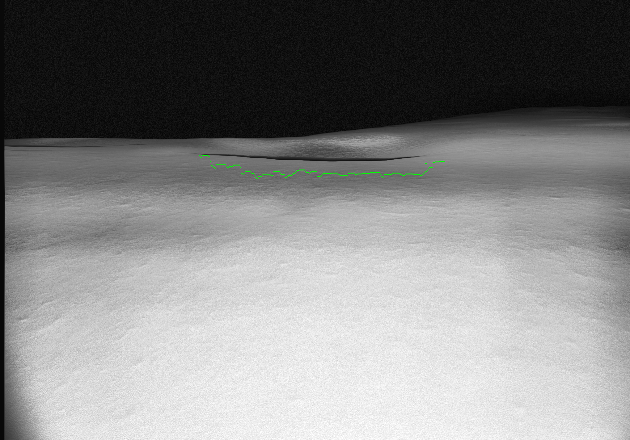
(v)

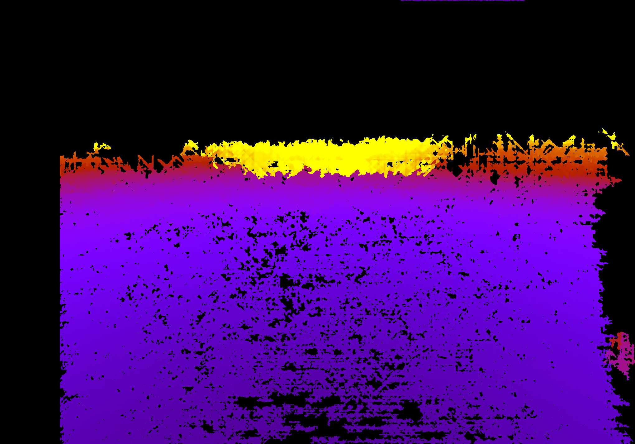
(w)

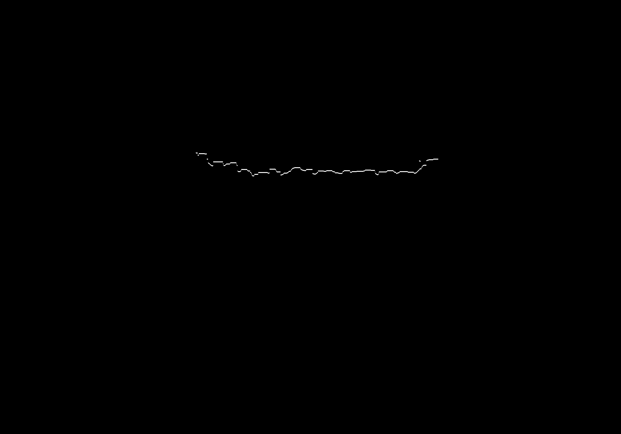
(x)

Figure 8: Samples of three main perception components. In the left column is the raw image. The left-middle column is the enhanced image with a green line to mark rim detections. The right-middle column is a colorized stereo range image. The right column is the crater rim detection mask. The top three samples are from Cinder Lakes and the bottom three samples are from the Lunar simulator.

One of the limitations of the above analysis is that all of the craters were mostly centered within the image frame. In this work, we assumed that highly accurate heading estimates are provided from, e.g., a star tracker and allow for centered detections with perfect absolute position. However, upon approaching a crater, there is an expected error in absolute position due to the drift of relative localization. In order to evaluate how these positional errors affect detection performance, data was rendered with a positional offset from the position that the ideal heading was determined from. This data is described in more detail in Section 4.1. Using this data, Figure 9 shows the results of Q-scores and detected rim percent results with a $5\text{\,}\mathrm{m}$ and $10\text{\,}\mathrm{m}$ horizontal shift. Only horizontal errors are plotted because forward/backward errors are captured as a shift along the x-axis in Figure 7. From Figure 9, we observed that $5\text{\,}\mathrm{m}$ horizontal offset has some degredation in crater matching performance but detection stays fairly similar. However, crater matching and detection degrades at less than $10\text{\,}\mathrm{m}$ range due to the crater not being captured within the field-of-view of the camera. Crater matching still degrades around $15\text{\,}\mathrm{m}$, but the degredation is similar to that of no positional offset. Overall crater detection and matching demonstrates strong performance within the $5\text{\,}\mathrm{m}$-$15\text{\,}\mathrm{m}$ range with potential for performance out to $20\text{\,}\mathrm{m}$ detection range.

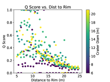
(a)

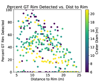
(b)

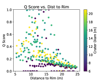
(c)

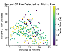
(d)

Figure 9: Crater detection and matching results with positional error on simulated data with a camera height of 2.5m a light offset of 20cm below camera, high brightness, and 1.2 pixel intensity sigma Gaussian noise to image (a) Q score 5m error (b) Percent detected 5m error (c) Q score 10m error (d) Percent detected 10m error.

5.3 Absolute Localization

Instantaneous perception measurements demonstrated strong performance in the previous section, but also presented some issues. Through the use of a particle filter approach outlined in Section 3.4, multiple perception measurements can be fused overtime to correct absolute position after it has drifted. In order to evaluate the performance of the absolute localization both simulation and Cinder Lakes data is used.

5.3.1 Simulation

Table 2: Localization results for all simulated trajectories with 2% added error using SGBM and discontinuity detection for perception.

Trajectory Distance (m) Num Landmarks Avg error (m) Stdev error (m) Max error (m) $>$ 5m error straight crater15 558 2 6.36 2.16 11.63 0.77 half survey crater15 617 2 3.75 1.28 5.40 0.13 full survey crater15 759 2 5.18 0.84 6.78 0.67 straight NtoS 665 2 4.81 2.56 9.01 0.50 half survey NtoS 714 2 2.12 1.16 5.95 0.07 full survey NtoS 840 2 2.08 0.97 4.22 0.00 straight StoN 536 2 7.65 2.63 11.29 0.70 half survey StoN 591 2 4.16 2.06 9.07 0.30 full survey StoN 726 2 3.10 2.58 10.39 0.13 traj 1km 1058 3 2.84 1.28 5.59 0.10 traj 1km rev 1211 3 4.34 2.02 8.84 0.33

First, evaluation is performed within simulation to determine the best trajectory to observe a landmark crater. This was accomplished by designing three types of trajectories around the same landmarks. The first trajectory type was a straight trajectory which stops every $10\text{\,}\mathrm{m}$ and travels directly past the crater with the nearest approach approximately $10\text{\,}\mathrm{m}$ from the rim. The second trajectory type was a half survey, which was designed so that observation positions occur 180 degrees around the crater with each observation point approximately $7\text{\,}\mathrm{m}$-$13\text{\,}\mathrm{m}$ from the crater rim. The third trajectory type was similar to half survey but had observation points a full 360 degrees around the crater. Table 2 contains the results for all trajectory types with a 2% error growth and Figure 10 is a histogram of final absolute errors of three different trajectories. For each trajectory, we performed Monte Carlo runs of 30 different tests and each test having a 2% relative localization error. From these results, we observed that the half survey and the full survey approaches perform much better than the straight trajectory which is expected. However, performing a full survey versus half survey does not provide additional benefit. The full survey does have some trajectories that perform better but in other trajectories it actually performs worse. Therefore, we believe that performing a half survey provides enough positional variance to constrain the localization.

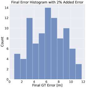
(a)

(b)

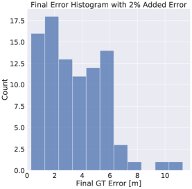
(c)

Figure 10: Simulation absolute localization histogram results with 2% error added for different trajectories near landmarks. (a) Straight trajectory (b) Survey half of crater rim (c) Survey full crater rim.

Next, varying error rates were observed within the simulated half survey trajectories. Figure 11 shows the results of experiments for 1%, 2%, and 3% added error. We observed that for 1% and 2% added error the localization is strong. However, with 3% added error, there are seven samples that violate the requirement of remaining below $10\text{\,}\mathrm{m}$ error. This reduction in performance is expected though as the performance is designed to recover from up to $10\text{\,}\mathrm{m}$ error. At 3% error over a $300\text{\,}\mathrm{m}$ traverse, there will be about $9\text{\,}\mathrm{m}$ of error added within our Monte Carlo runs. The filter is only able to localize reliably within  $5\text{\,}\mathrm{m}$ and this potentially allows for the absolute error to increase beyond  $10\text{\,}\mathrm{m}$ at the second landmark.

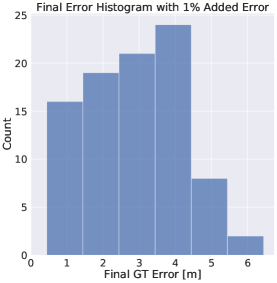
(a)

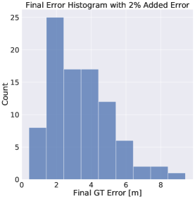
(b)

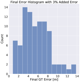
(c)

Figure 11: Simulation absolute localization histogram results for the half survey trajectories. (a) 1% error added (b) 2% error added (c) 3% error added

Finally, a trajectory $\geq$$1\text{\,}\mathrm{km}$ trajectory was tested with three landmarks and involved running the trajectory forwards and backwards with half surveys of each landmark. The results for this trajectory are also in Table 2. Overall, results from the $1\text{\,}\mathrm{km}$ trajectory demonstrate that the particle filter can maintain stability across more landmarks and longer trajectories.

5.3.2 Cinder Lakes

Table 3: Localization results for all Cinder Lakes trajectories with 2% added error using SGBM and discontinuity detection for perception. Error metrics are the absolute error at the final position of the trajectory.

Trajectory Distance (m) Num Landmarks Avg error (m) Stdev error (m) Max error (m) $>$ 5m error south_NtoS 280 1 2.62 0.99 4.86 0.00 south_vA 568 2 1.89 0.90 3.82 0.00 south_vA_rev 568 2 3.86 1.66 7.57 0.27 south_vA_5loop 4419 10 12.97 14.95 57.01 0.40 north_NA12_NM12 424 2 2.71 1.23 5.41 0.03 north_ND1_NA12_NM12 424 3 3.02 1.63 6.43 0.10 north_ND1_NA12_NM12_rev 491 3 3.44 1.81 6.25 0.33 north_ND1_NM12 424 2 4.81 2.36 8.11 0.53 north_ND1_NA12_rev 491 2 3.26 1.84 6.45 0.23 north_ND1_NM12_rev 491 2 4.50 2.24 8.48 0.53

Next, we utilized the trajectories collected at Cinder Lakes to validate absolute localization in an analogue Lunar environment. For evaluation, we used a total of three trajectories with two from the South site and one from the north site. One of the south site trajectories, south_vA was connected via artificial points to make it a loop. There is no image data at the locations but the error grows with the distance. This loop utilizes the same image data repeatedly, but allows for a simulation of stability. For the north site trajectory, different combinations of landmarks were utilized with two to three landmarks utilized during each run. The full results of these trajectories with 2% added error are in Table 3. We observed that performance is solid except for the looping trajectory. Additionally, we observed that the filter experienced issues in attaining absolute errors less than $5\text{\,}\mathrm{m}$ along one of the north site trajectories. Figure 12 presents a comparison of the actual trajectory with 2% added error compared with the looped trajectory at 1% and 2% added error. It is shown that there is roughly $400\text{\,}\mathrm{m}$ between craters. With one traverse, the localization can recover from a $10\text{\,}\mathrm{m}$ error. However, we observed that the max error grows while running multiple loops with 2% error and the filter diverges. However, with multiple loops and 1% error, the max error does not grow and the filter maintains stability. Given these results, we can determine that error growth between landmarks should be no more than $5\text{\,}\mathrm{m}$-$6\text{\,}\mathrm{m}$ error and the length of traverses between landmarks can be subsequently developed by assumming 2% relative localization error.

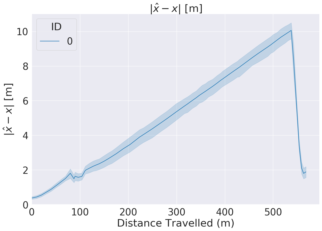
(a)

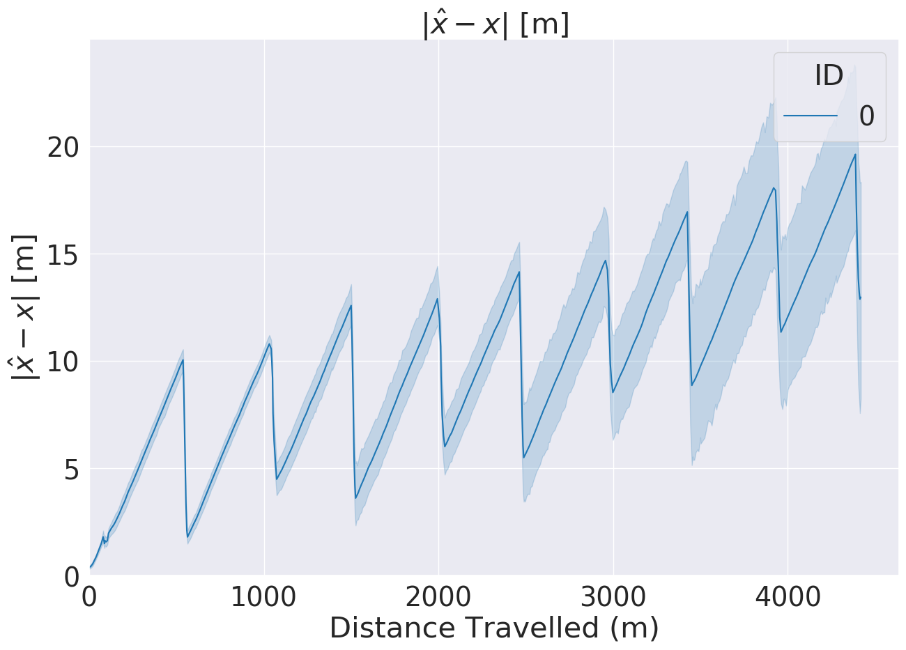
(b)

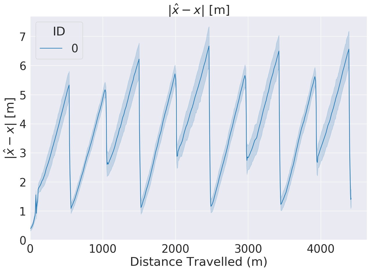
(c)

Figure 12: Cinder Lakes crater absolute localization results for a single trajectory, south_vA. (a) 1 time through trajectory with 2% error added (b) 5 loops through trajectory with 2% error added (c) 5 loops through trajectory with 1% error added.

Furthermore, the other non-looped trajectories were run for 1%, 2%, and 3% added error rates. The results are shown in Figure 13 and, consistent with our findings in simulation, we observed filter divergence with increased relative error. However, with 1% and 2% error rates, the absolute localization is able to consistently localize within $5\text{\,}\mathrm{m}$ final error and contain no samples greater than $10\text{\,}\mathrm{m}$ final error.

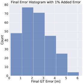
(a)

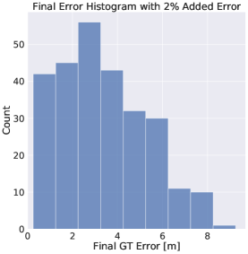
(b)

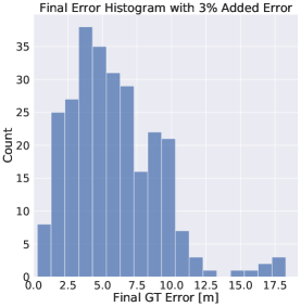
(c)

Figure 13: Cinder Lakes crater absolute localization histogram results for single loop trajectories. (a) 1% error added (b) 2% error added (c) 3% error added

5.4 Benchmark on Flight-Like Computer

Table 4: Perception computation results on a single core of a Snapdragon 8155

Dataset	Resolution	SGBM max (sec)	Detect max (sec)
Cinder Lakes	1295x602	0.48	0.25
Simulation	2039x1425	4.40	0.91

Table 5: Localization step computation results on a single core of a Snapdragon 8155.

Dataset	Num. Particles	PF step avg. [seconds]	Pf step max [seconds]
Cinder Lakes	50	1.49	2.17
Cinder Lakes	100	2.96	4.29
Cinder Lakes	200	6.00	8.71
Simulation	50	1.71	2.78
Simulation	100	3.41	5.56
Simulation	200	6.96	11.16

In this section, we demonstrate that the proposed ShadowNav approach is capable of being run onboard a flight mission and benchmark our algorithm on a Snapdragon 8155 processor. First, the perception algorithms of SGBMs stereo and discontinuity detection were evaluated and the results are in Table 4. Table 5 shows the results of benchmarking these localization algorithms across a range of several different parameters. The Endurance-A proposal concept [Keane et al., 2022] calls for having the rover stop for approximately ten minutes between drives in order to perform absolute localization. Additionally, long exposure captures are proposed to be captured every $10\text{\,}\mathrm{m}$. Therefore, for a $300\text{\,}\mathrm{m}$ traverse, there could be on the order of 30 iterations to process. In the worst case, a filter using 200 particles would be able to terminate its particle filtering calculation within 8.5 minutes. However, the average case should terminate faster and fulfill the ConOps requirement. The other consideration is to support processing while driving. The Endurance-A concept also proposed 1 minute stops every $10\text{\,}\mathrm{m}$ for the long exposures that this system would use. The perception could likely run during this stop along with potentially the absolute localization processing depending upon other processing needs. Additionally, there is at 20 seconds of driving between long exposures during which a single core could potentially be allocated to perform the localization step. Therefore, we believe that the computation requirements of this system are suitable for use onboard.

6 Conclusion

In this work, we presented an autonomous absolute localization framework for a Lunar rover mission driving at night or in dark regions of the Moon. Our approach consists of using the leading edges of craters as landmarks and matching these detected craters with known Lunar craters from an offline map. We validated our proposed approach in a simulation environment created using Blender and data collected from a field test conducted at Cinder Lakes. Future contributions will focus on how the proposed ShadowNav approach would perform within a full system that is running relative localization on-board. A further area of exploration is the problem of recovering from errors errors greater than $10\text{\,}\mathrm{m}$ or to contain an understanding of faults to know if the system was unable to localize. Finally, the system should be evaluated with absolute localization in the loop over long distances to ensure stability.

References

- Arulampalam et al., 2002 Arulampalam, M. S., Maskell, S., Gordon, N., and Clapp, T. (2002). A tutorial on particle filters for online nonlinear/non-Gaussian Bayesian tracking. IEEE Transactions on Signal Processing, 50(2):174–188.
- Bhamidipati et al., 2023 Bhamidipati, S., Mina, T., Sanchez, A., and Gao, G. (2023). Satellite constellation design for a lunar navigation and communication system. NAVIGATION, 70(4).
- Cauligi et al., 2023 Cauligi, A., Swan, R. M., Ono, H., Daftry, S., Elliott, J., Matthies, L., and Atha, D. (2023). ShadowNav: Crater-based localization for nighttime and Permanently Shadowed Region Lunar navigation. In IEEE Aerospace Conference.
- Cisneros et al., 2017 Cisneros, E., Awumah, A., Brown, H. M., Martin, A. C., Paris, K. N., Povilaitis, R. Z., Boyd, A. K., Robinson, M. S., and LROC Team (2017). Lunar Reconnaissance Orbiter camera permanently shadowed region imaging – atlas and controlled mosaics. In Lunar and Planetary Science Conference.
- Cortinovis et al., 2024 Cortinovis, M., Mina, T., and Gao, G. (2024). Assessment of single satellite-based lunar positioning for the NASA Endurance Mission. In IEEE Aerospace Conference.
- Crues et al., 2023 Crues, E. Z., Bielski, P., Paddock, E., Foreman, C., Bell, B., Raymond, C., Hunt, T., and Bulikhov, D. (2023). Approaches for validation of lighting environments in realtime Lunar South Pole simulations. In IEEE Aerospace Conference.
- Daftry et al., 2023 Daftry, S., Chen, Z., Cheng, Y., Tepsuporn, S., Khattak, S., Matthies, L., Coltin, B., Naam, U., Ma, L. M., and Deans, M. (2023). LunarNav: Crater-based localization for long-range autonomous rover navigation. In IEEE Aerospace Conference.
- Franchi and Ntagiou, 2022 Franchi, V. and Ntagiou, E. (2022). Planetary rover localisation via surface and orbital image matching. In IEEE Aerospace Conference.
- Hapke, 2002 Hapke, B. (2002). Bidirectional reflectance spectroscopy: 5. the coherent backscatter opposition effect and anisotropic scattering. Icarus, 157(2):523–534.
- Hapke, 2012 Hapke, B. (2012). Theory of reflectance and emittance spectroscopy. Cambridge Univ. Press.
- Hiesinger et al., 2012 Hiesinger, H., van der Bogert, C. H., Pasckert, J. H., Funcke, L., Giacomini, L., Ostrach, L. R., and Robinson, M. S. (2012). How old are young lunar craters? Journal of Geophysical Research, 117(12):1–15.
- Hirschmuller, 2007 Hirschmuller, H. (2007). Stereo processing by semiglobal matching and mutual information. IEEE Transactions on Pattern Analysis & Machine Intelligence, 30(2):328–341.
- Hwangbo et al., 2009 Hwangbo, J. W., Di, K., and Li, R. (2009). Integration of orbital and ground image networks for the automation of rover localization. In American Society for Photogrammetry and Remote Sensing Annual Conference.
- Johnson et al., 2008 Johnson, A. E., Goldberg, S. B., Cheng, Y., and Matthies, L. H. (2008). Robust and efficient stereo feature tracking for visual odometry. In Proc. IEEE Conf. on Robotics and Automation.
- Keane et al., 2022 Keane, J. T., Tikoo, S. M., and Elliott, J. (2022). Endurance: Lunar South Pole-Atken Basin traverse and sample return rover. Technical report, National Academy Press.
- Klear, 2018 Klear, M. R. (2018). PyCDA: An open-source library for automated crater detection. In Planetary Crater Consortium.
- Kogan, Kogan, D. mrcal. http://mrcal.secretsauce.net.
- Liounis et al., 2019 Liounis, A., Swenson, J., Small, J., Lyzhoft, J., Ashman, B., Getzandanner, K., Highsmith, D., Moreau, M., Adam, C., Antreasian, P., and Lauretta, D. S. (2019). Independent optical navigation processing for the OSIRIS-REx mission using the Goddard Image Analysis and Navigation Tool. In RPI Space Imaging Workshop.
- Maimone et al., 2007 Maimone, M., Cheng, Y., and Matthies, L. (2007). Two years of visual odometry on the Mars Exploration Rovers. Journal of Field Robotics, 24(3):169–186.
- Maimone et al., 2022 Maimone, M., Patel, N., Sabel, A., Holloway, A., and Rankin, A. (2022). Visual odometry thinking while driving for the Curiosity Mars rover’s three-year test campaign: Impact of evolving constraints on verification and validation. In IEEE Aerospace Conference.
- Matthies et al., 2022 Matthies, L., Daftry, S., Tepsuporn, S., Cheng, Y., Atha, D., Swan, R. M., Ravichandar, S., and Ono, M. (2022). Lunar rover localization using craters as landmarks. In IEEE Aerospace Conference.
- National Academies of Sciences, Engineering, and Medicine, 2022a National Academies of Sciences, Engineering, and Medicine (2022a). INSPIRE (IN situ Solar system Polar Ice Roving Explorer): A mission concept study from the Decadal Survey for Planetary Science and Astrobiology 2022–2032. Technical report, National Academy Press.
- National Academies of Sciences, Engineering, and Medicine, 2022b National Academies of Sciences, Engineering, and Medicine (2022b). Origins, worlds, and life: A decadal strategy for planetary science and astrobiology 2023–2032. Technical report, National Academy Press.
- Robinson and Elliott, 2022 Robinson, M. and Elliott, J. (2022). Intrepid planetary mission concept study report. Technical report, National Academy Press.
- Robinson et al., 2010 Robinson, M. S., Brylow, S. M., Tschimmel, M., Humm, D., Lawrence, S. J., Thomas, P. C., Denevi, B. W., Bowman-Cisneros, E., Zerr, J., Ravine, M. A., Caplinger, M. A., Ghaemi, F. T., Schaffner, J. A., Malin, M. C., Mahanti, P., Bartels, A., Anderson, J., Tran, T. N., Eliason, E. M., McEwen, A. S., Turtle, E., Jolliff, B. L., and Hiesinger, H. (2010). Lunar Reconnaissance Orbiter (LROC) camera instrument overview. Space Science Reviews, 150.
- Scharstein et al., 2001 Scharstein, D., Szeliski, R., and Zabih, R. (2001). A taxonomy and evaluation of dense two-frame stereo correspondence algorithms. In Proc. IEEE Workshop on on Stereo and Multi-Baseline Vision.
- Schmidt and Bourguignon, 2019 Schmidt, F. and Bourguignon, S. (2019). Efficiency of BRDF sampling and bias on the average photometric behavior. Icarus, 317:10–26.
- Silburt et al., 2019 Silburt, A., Ali-Dib, M., Zhu, C., Jackson, A., Valencia, D., Kissin, Y., Tamayo, D., and Menou, K. (2019). Lunar crater identification via deep learning. Icarus, 317:27–38.
- Silvestrini et al., 2022 Silvestrini, S., Piccinin, M., Zanotti, G., Brandonisio, A., Bloise, I., Feruglio, L., Lunghi, P., Lavagna, M., and Varile, M. (2022). Optical navigation for lunar landing based on convolutional neural network crater detector. Aerospace Science and Technology, 123:107503.
- Verma et al., 2023a Verma, V., Maimone, M., Graser, E., Rankin, A., Kaplan, K., Myint, S., Huang, J., Chung, A., Davis, K., Tumbar, A., Tirona, I., and Lashore, M. (2023a). Results from the first year and a half of Mars 2020 robotic operations. In IEEE Aerospace Conference.
- Verma et al., 2023b Verma, V., Maimone, M. W., Gaines, D. M., Francis, R., Estlin, T. A., Kuhn, S. R., Rabideau, G. R., Chien, S. A., McHenry, M., Graser, E. J., Rankin, A. L., and Thiel, E. R. (2023b). Autonomous robotics is driving Perseverance rover’s progress on Mars. Science Robotics, 8(80):1–12.
- Woicke et al., 2018 Woicke, S., Moreno Gonzalez, A. S., El-Hajj, I., Mes, J. W. F., Henkel, M., Autar, R. S. D., and Klavers, R. A. (2018). Comparison of crater-detection algorithms for terrain-relative navigation. In AIAA Conf. on Guidance, Navigation and Control.
- Wu et al., 2019 Wu, B., Potter, R. W. K., Ludivig, P., Chung, A. S., and Seabrook, T. (2019). Absolute localization through orbital maps and surface perspective imagery: A synthetic lunar dataset and neural network approach. In IEEE/RSJ Int. Conf. on Intelligent Robots & Systems.
- Xu et al., 2020 Xu, X., Liu, J., Liu, D., Liu, B., and Shu, R. (2020). Photometric correction of Chang’E-1 interference imaging spectrometer’s (IIM) limited observing geometries data with Hapke model. Remote Sensing, 12(22):3676.
- Yadav et al., 2014 Yadav, G., Maheshwari, S., and Agarwal, A. (2014). Contrast limited adaptive histogram equalization based enhancement for real time video system. In Proc. IEEE Int. Conf. on Advances in Computing, Communications and Informatics .
- Zhang et al., 2020 Zhang, F., Qi, X., Yang, R., Prisacariu, V., Wah, B., and Torr, P. (2020). Domain-invariant stereo matching networks. In European Conf. on Computer Vision.