Multi-filter UV to NIR Data-driven Light Curve Templates for Stripped Envelope Supernovae

Abstract

While the spectroscopic classification scheme for Stripped envelope supernovae (SESNe) is clear, and we know that they originate from massive stars that lost some or all their envelopes of Hydrogen and Helium, the photometric evolution of classes within this family is not fully characterized. Photometric surveys, like the Vera C. Rubin Legacy Survey of Space and Time, will discover tens of thousands of transients each night and spectroscopic follow-up will be limited, prompting the need for photometric classification and inference based solely on photometry. We have generated 54 data-driven photometric templates for SESNe of subtypes IIb, Ib, Ic, Ic-bl, and Ibn in ${U/u,~{}B,~{}g,~{}V,~{}R/r,~{}I/i}$, ${J,~{}H,~{}K_{s}}$, and Swift ${w2,~{}m2,~{}w1}$ bands using Gaussian Processes and a multi-survey dataset composed of all well-sampled open-access light curves (165 SESNe, 29531 data points) from the Open Supernova Catalog. We use our new templates to assess the photometric diversity of SESNe by comparing final per-band subtype templates with each other and with individual, unusual and prototypical SESNe. We find that SNe Ibn and Ic-bl exhibit a distinctly faster rise and decline compared to other subtypes. We also evaluate the behavior of SESNe in the PLAsTiCC and ELAsTiCC simulations of LSST light curves highlighting differences that can bias photometric classification models trained on the simulated light curves. Finally, we investigate in detail the behavior of fast-evolving SESNe (including SNe Ibn) and the implications of the frequently observed presence of two peaks in their light curves.

1 Introduction

Stripped envelope supernovae (SESNe) include a diverse ensemble of explosive transients that arise from the core collapse of massive stars that have been stripped of various amounts of their outer layers before explosion. Their distinctive observational signature is the absence (or weakness) of hydrogen (H) in their maximum light spectra, and this family of transients includes SNe type Ib and IIb, SNe type Ic and Ic-bl, which also lack signatures of helium (He), and their subtypes (Clocchiatti & Wheeler, 1997; Filippenko, 1997; Gal-Yam, 2016; Modjaz et al., 2019) including the “transitional” type Ibn (Pastorello et al., 2015). While intrinsically nearly as common as Type Ia SNe (Shivvers et al., 2016) they are less luminous, and, unlike SNe Ia, SESNe do not show phenomenological relationships that can be exploited for standardization; thus, they are not an obvious cosmological tool (although some of the subtypes, especially SNe Ic-bl with GRB, have been claimed to be promising standardizable candles, see Cano 2014, and references therein). For these reasons they are less observed and less well-studied than SNe Ia, and since they are relatively less common, less observed than SNe II.

In 2014, our groups presented what is still today one of the largest homogeneous photometric sample of SESNe, Bianco et al. (2014) – B14 hereafter – complemented by currently one of the largest spectroscopic samples, Modjaz et al. (2014) – M14 hereafter. Both of these works are based on the CfA SN Survey, comprising 64 photometric targets, and 73 spectroscopic targets, of which 54 are in both samples and we began addressing the observational photometric properties of the SESNe population. Our work was followed by the data releases and analysis of Stritzinger et al. (2018a) – CSP hereafter – and Stritzinger et al. (2018b) – based on the Carnegie Observatory data (CSP), and more recently the Palomar Transient Factory (PTF) and intermediate PTF (iPTF) data that supported studies including Vincenzi et al. (2019), Schulze et al. (2021), and Barbarino et al. (2021), although a formal data release for these SESNe is still to come. Currently, fewer than 150 objects comprise a heterogeneous sample of well-studied SESNe released in different publications (Drout et al. 2011 – D11 hereafter –, Cano 2013a, M14, B14 , Lyman et al. 2016; Prentice et al. 2016; Modjaz et al. 2014; Liu et al. 2016; Stritzinger et al. 2018a, , Sollerman et al. 2021; Ho et al. 2023 – hereafter Ho23).

Our work is motivated by two distinct goals. In the era of large photometric surveys, like the Vera C. Rubin Legacy Survey of Space and Time, hereafter LSST (Ivezić et al., 2019), increasing emphasis has to be placed on photometric classification and characterization of transients and variable phenomena, as spectroscopic resources will only enable follow up of a small fraction of observed transients (Najita et al., 2016). With this motivation, photometric classifiers of astrophysical transients, even from sparse light curves, have seen rapid developments (see for example Qu & Sako 2022, and references therein; Hložek et al. 2020, and references therein). More recent work is emerging approaching classification from a more holistic perspective, for example, using photometry jointly with galaxy host information Gagliano et al. (2023). Yet, primarily, the focus and drive for these works have been to ensure the purity of cosmological SN Ia samples in high-$z$ synoptic surveys, rather than understanding the properties and diversity of SESNe and setting the stage for SESNe physics and stellar evolution studies in an astronomical era with an unprecedented wealth of photometry, but when spectra of the photometric transients will be rare. As an example, some of the most successful supernova photometric classifiers, like Boone (2019) or Qu & Sako (2021), to name just two, achieve $>80\%$ accuracy on the classification of SNe Ia, but for even for SESNe as a collective class, they obtain modest classification power (52% accuracy for Boone 2019 and as good as 78% for Qu & Sako 2021 but only when a full light curve up to 50 days after discovery is used and accurate spectral information is available to measure the redshift). We note that both these studies are based on the PLAsTiCC challenge dataset (Kessler et al., 2019) and we will compare this simulated dataset, and its successor ELAsTiCC, with our observations in subsection 5.5 to assess the accuracy of SN Ibc simulated sample, and discuss implications for machine learning models trained on these data.

Our ultimate goal is to assess the photometric diversity of SESNe, among and within subtypes, setting the stage for studies aimed at relating the explosion taxonomy to diversity in explosion properties and progenitor rates. This inference requires several steps to extract the underlying physics of the explosions from the observed explosion properties. On the way to achieve our stated goal, in this paper, we will address the generation of data-driven templates for SESNe subtypes, with a focus on addressing methodological challenges and designing best practices in the selection of the data on which the templates are based, and care in the algorithmic choices that minimize the introduction of biases in the template.

As the authors strongly believe in the benefit of open science and open data, we chose to use the Open Supernova Catalog (Guillochon et al., 2016, hereafter OSNC) as the backbone of our study; all SNe included in our work are sourced from this open library, or we contributed them this library, with a few instances in which the data from OSNC was augmented or corrected based on data available to the authors or published but not integrated in the catalog and for which we submitted pull requests though the OSNC GitHub project. However, unfortunately, in the time span over which this paper was written, the OSNC stopped being regularly maintained, as it happens to a significant fraction of open software and data portals (Nowogrodzki, 2019). The interactive part of the OSNC broke down on March 8 2022 irrecoverably, and it is now only accessible through its API and GitHub. We will discuss the benefits of, and difficulties encountered in, using an open dataset, rather than a proprietary dataset owned by the authors or accessed through a colleague’s network.

Data-driven spectral templates of SESN, or mean spectra, have been published in Liu et al. (2016) and Modjaz et al. (2014) and lead to an improved understanding of the subtypes’ typical characteristics, and of the relation between subtypes. Additionally, photometric templates of SESNe were produced by D11, Taddia et al. (2015, T15 hereafter), and Vincenzi et al. (2019) and SN Ibn templates by Hosseinzadeh et al. (2017, H17 hereafter) that we will discuss and compare to ours in subsection 4.1 and subsection 5.4.

We present here data-driven light curve templates for all bands from ultraviolet (UV) to near-infrared (NIR) separately, which will allow us to correct for incomplete observations when generating bolometric light curves in future work and allow us to probe the characteristics of the photometric evolutions of SESNe. After discussing relevant literature and our motivations (section 2) and the data that supports our work (section 3), we present two sets of templates we develop. The SN Ibc templates are rolling median templates made for each band using all SNe in our sample, introduced and discussed in section 4. These are also used to support the creation of templates created using Gaussian Processes (GP) for each SESNe subtype separately in each band (section 5). We compare our templates with templates for SESN produced by other authors, individual objects that we found or are thought to be peculiar and prototypical, and synthetic samples used in the literature for model development (subsection 4.1 and subsection 5.4), and we examine in detail the photometric evolution of rapid evolving SESNe (subsection 5.7 and subsection 5.8). Our conclusions are summarized in section 6. Our work is reproducible and we make available to the reader the templates produced with our curated photometric sample as well as the methods and code we developed to generate and update templates as observations of new SNe become available..

2 Supernova Templates: Motivation and Status of the Field

In this work, we generated two sets of templates for stripped-envelope supernovae:

• a set of SN Ibc templates that describe the behavior of the SESNe as a single family (although we know that there are differences in the subtype phenomenology!), one for each photometric band in ${U,u,~{}B,~{}g,~{}V,~{}R,~{}r,~{}I,~{}i}$, ${J,~{}H,~{}K_{s}}$, and Swift UV ${w2,~{}m2,~{}w1}$. Using all subtypes together allows the sample to be large enough to successfully generate templates in all but the UV bands. We discuss these templates first in section 4.

• individual subtype templates for SN type IIb, Ib, Ic, Ic-bl, and Ibn in individual bands. Constructing these templates requires a Bayesian approach (GP) and templates can only be produced in some bands. However, these templates enable the assessment of similarities and differences in the photometric evolution of different SESN subclasses. These will be referred to as final templates or GP templates and will be discussed in more detail in section 5.

Light curve templates are instrumental in most inference one may envision doing on and with SNe. In our case, our first goal is to understand diversity, with the final aim to relate the diversity of explosion to different progenitors, and to be able to identify the presence of separate classes vs a continuum in the range of observed properties.

Spectral templates of stripped SNe have been published in Liu et al. (2016) and Modjaz et al. (2014), leading to an improved understanding of the subtypes’ typical characteristics, and of the relationship between subtypes. Photometric templates are often derived from a single well-observed SN (e.g. Cano, 2013b) or combined from small samples of objects from a single survey (e.g. Drout et al., 2011). More recently Vincenzi et al. (2019) produced single-object spectro-photometric templates for 67 core-collapse (CC) SNe, including 37 SESNe.

The time behavior of SN light curves has been modeled from physical principles by many authors; just a few examples are the seminal work of Arnett 1982, and more recent work including Bernstein et al. 2012, Piro 2015, and Orellana & Bersten 2022,. The simplest, most general data-driven functional form is provided by Vacca & Leibundgut (1996) and Vacca & Leibundgut (1997), which models the light curves of SNe with an exponential rise, a Gaussian peak, and a linear decay (and a secondary peak if needed, as, for example, in red optical and NIR bands for SNe Ia). For standard SN light curves, this parameterization can be very successful. However, it may fail to model subtle peculiarities of a SN, and, generally, we expect the above model to capture most of the variation in thermonuclear SNe Ia, but other types of SNe, such as our SESNe, show more diversity. Therefore, we focus on a non-parametric data-driven model in this paper.

Most models from which one can obtain explosion parameters rely on bolometric flux information (e.g. Arnett 1982). However, we observe our SNe in individual photometric bands, occasionally obtaining observations throughout a large portion of the photometric spectrum, from UV through IR, only exceptionally even pushing into the X-ray and Radio, but more often in just a much narrower portion of the spectrum: optical, or optical and NIR. In this work, we create single-band templates for SESNe in as many bands as the data allows, with a comprehensive dataset that aspirationally includes all SESN photometric data available in the literature (section 3). Producing bolometric light curves from these data and templates also requires that one corrects for dust extinction in both our and the host galaxies, which remains, in spite of recent attempts to find empirical relationship (Stritzinger et al., 2018b), an unresolved issue for transients that, like SESN, are not standardizable (i.e., for which we do not know the un-extincted behavior). Uncertain host galaxy extinction remains the largest source of uncertainty in the derivation of absolute parameters from observed explosions. The creation of light curve templates in each photometric band separately does not require extinction correction. In each band, we only use the relative magnitude, so that neither a color correction nor the absolute luminosity are needed (see also section 3). In other words, we create photometric magnitude templates by combining individual SNe relative photometry. Our photometric templates, then, are designed to have the same peak brightness in each band (nominally 0) to describe the shape of the light curve for each subtype, and its evolution. Therefore, we will work with relative magnitude throughout the paper and we do not deal with the diversity in the absolute magnitude of the SESNe.

These templates pave the way to address a core open question about SESNe: what is the relation between subtypes, and are we indeed seeing distinct classes, arising from quantitatively distinct progenitors and/or explosion mechanisms, or are we in the presence of a continuum of observational properties that indicate a gap-less evolution between progenitor properties and similar explosion mechanisms: in other words, is the progenitor mass the only difference between stars that explode as SN Ib, vs SN Ic, or do environment and mechanisms for the ejection of the material prior to explosion differ?

A word of caution is necessary: templates are statistical aggregates. In the presence of gappy or incomplete light curves, we can use templates to input missing data, but we run the risk of biasings ourselves to the aggregate behavior and impose homogeneity. So while templates can assist us in answering questions about progenitors, we must strive to construct templates that respect the diversity within the sample. Using the largest possible dataset and paying exquisite attention to uncertainties in the data and in the interpolation assures we represent the distribution of our data as well as the dataset allows, and this is what we strived toward in this work.

3 Data

A data-driven template requires a sufficient amount of data to capture the details and the diversity of a phenomenon, and until recently, the field of SESNe has suffered from a significant scarcity of data. However, the sample of observed SESNe bloomed in recent years. Like any astronomical transient phenomenon, the dataset grew rapidly with the advent of optical sky surveys, starting with SDSS (although these SESNe are not always “well-observed”). Our study is enabled by the existence of the Open Supernova Catalog (OSNC Guillochon et al., 2016). The OSNC was a platform, part of the Open Astronomy Catalogs GitHub organization, an effort to catalog and digitize all SNe observed (and whose observations have been published) into a single consistent repository. It collected and digitized all SN photometry and spectroscopy. Sadly, the OSNC catalog is no longer maintained and the OSNC has been frozen as-is on April 8, 2022. We regret the loss of this legacy. This study leverages the unique collection of SESNe in the OSNC which represents our collective (nearly) complete data knowledge of SESNe as of the early 2020s.

Figure 1 shows the number of SESNe discovered since the first hydrogen-poor SN Ib was discovered in 1954 (SN 1954A, Pietra 1955). The top panel includes all SNe labeled as any SESN subtype, including general SN Ibc classifications and peculiar subtypes (e.g.: Ib-Pec, Ibn, Ca-rich Ib, but no He-poor super-luminous SNe - SLSN), while further into the project we will limit our sample to well-identified and generally non-peculiar subtypes. In the bottom panel we show only SNe with at least 10 photometric data points and at least one spectrum, as a first, crude cut to separate “well-observed” SNe (308 SESNe). The color bar in the bottom panel indicates the size of the best photometric sample of SESNe discovered per year.

We collected all photometry available in the OSNC as described above, and had also contributed to OSNC by augmenting the catalog, which was an open-source catalog and relied partially on the community data input. Two surveys contribute the bulk of the data that will be used in our work: CfA SN survey (B14) and the Carnegie Supernova Project (CSP Stritzinger et al. 2018a, b, c).

The CfA SN survey contributed to the literature collection of “well-observed” SESNe (i.e., with multiple photometric bands, and several spectra for each object to confirm classification and assess evolution) by doubling the existing sample (M14 and B14), with 4,543 optical measurements on 61 SNe and 1,919 NIR measurements on 25 SNe.

The Carnegie Supernova Project (CSP) released data for 34 supernovae, in optical and NIR bands ($u^{\prime},~{}B,~{}V,~{}g^{\prime},~{}r^{\prime},~{}i^{\prime},~{}Y,~{}H,~{}K_{s}$) with nearly 3,000 optical data points and nearly 700 NIR data points. Of these, 10 SNe had no previously published optical photometry. Half of the CSP sample (18 out of 34 SNe) already had published CfA photometry in B14, and the photometric measurements are generally in excellent agreement between the two surveys, with generally comparable uncertainties. The CSP sample is a smaller dataset by number of objects compared to B14 (34 objects compared to 62), although the size of the NIR samples is identical (25 SNe). Altogether, the surveys are comparable in sampling, CSP averaging 88 optical data points and 27 NIR data points per SN, compared to 73 and 77 respectively for B14.

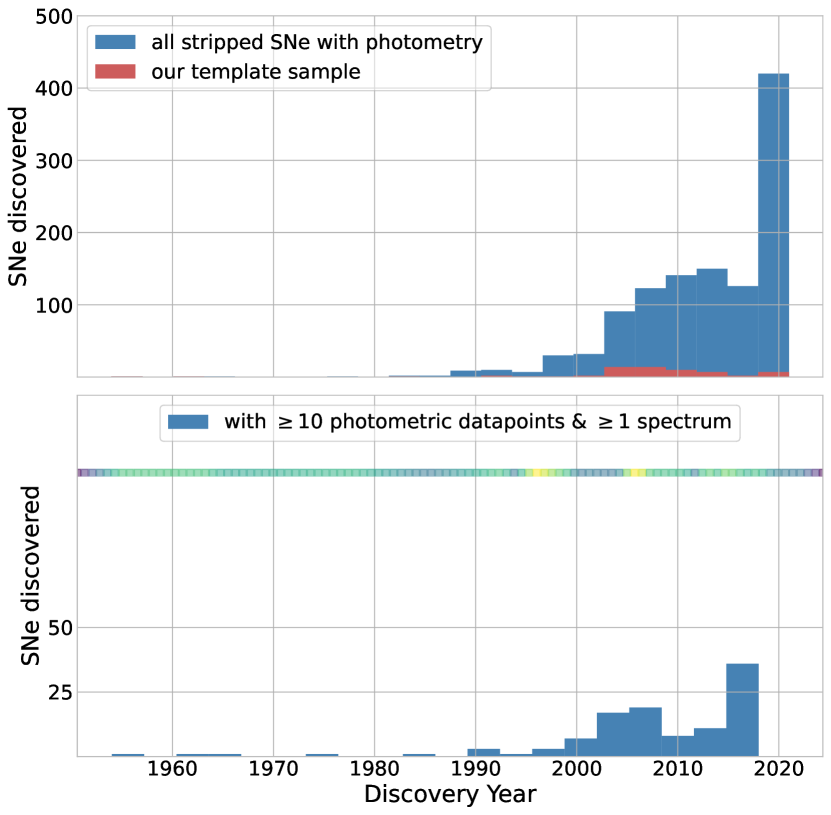
Figure 1: SESN discoveries since the first ${H}$-poor SN, SN 1954A (Pietra, 1955). The top panel shows all SESNe, including SNe Ibc and peculiar subtypes (but excluding SLSNe) and the bottom panel shows only SNe for which $>10$ photometric data points have been published. The color band running at the top of the bottom panel represents the average number of photometric data points per SN, in log scale, and it runs from a minimum (purple) of 0 in years when no SNe were observed to a maximum (yellow) of 1838 data points in 1993, with the single best observed SESNe: SN 1993J. The maximum number of discoveries with $>10$ photometric data points is reached in the five-year bin centered on 2004, but it is likely an artifact due to delayed publication: photometric observations often continue to appear in the literature in the decade following an object’s discovery.

D11 published the first pioneering survey on SESNe, including 25 objects observed in $V$ and $R$ bands. However, as shown in B14, this survey’s photometry can be contaminated by galaxy light due to D11’s extraction method (aperture photometry, instead of template subtraction). While a subset of the D11 SNe is likely minimally contaminated, most of the D11 objects were also observed in the B14 and CSP samples. Therefore, without loss of representation, we can remove these photometric data points from the sample we use to generate templates.

Taddia et al. (2015) introduced a sample of 20 SESN in a study of early lightcurves behavior.

Finally, the ZTF Bright Transient Survey, described in (Perley et al., 2020) also observed and released light curves for SESN starting in 2018. Objects from this survey are included if they were integrated in the OSNC. Many additional recent publications include individual SESNe and describe properties of the SESNe as a family (e.g. Vincenzi et al., 2019; Schulze et al., 2021) based on PTF, iPTF, and ZTF (Law et al., 2009; Kulkarni, 2013; Bellm et al., 2018) data. However, these data are yet to be released as an ensemble. The individual SNe published in the aforementioned publications are typically available and in many cases have been ingested into the OSNC, in which cases they are included by default in our work.

In summary, the final photometric data sample used for our templates comprises data from the large SESNe observing programs by CfA (B14) and CSP, individually published PTF/iPTF objects (e.g., iPTF13bvn, PTF11qcj, and PTF12hni), as well as other single object campaigns that produced well-observed SESNe (e.g., SN 1993J). Objects from PTF and iPTF also include: iPTF15dld, iPTF15dtg, PTF10qts, PTF11kmb, PTF12gzk, and SN 2016hgs (iPTF16hgs) (See subsubsection 3.1.3).

A collection of rapidly evolving SESNe from the ZTF survey was recently published by Ho23. This is a sample selected specifically because of its fast-evolving photometric signature so it is inherently a biased sample. Therefore we do not include SESN type SN Ib, SN IIb, SN Ic from this sample in the construction of our templates, rather we compare the photometric properties of this sample with our template (subsection 5.8). We do, however, include SN Ibn from Ho23 in the construction of our SN Ibn template as the expectation is that this subtype of SESNe is intrinsically rapidly evolving, so that the sample may be representative. These ZTF events are in fact included in the OSNC but do not appear to have spectra on the OSNC and therefore are automatically removed by our selection criteria (see subsection 3.1).

Finally, in a few cases, we included SESNe in our sample that had photometry missing from OSNC or their photometry was published in non-standard formats. These objects include SN 2010as, OGLE16ekf, iPTF15dld, PTF10qts, SN 1999dn, and SN 2002ji (Folatelli et al., 2014; Pian et al., 2017; Walker et al., 2014; Benetti et al., 2011). Also, DES16S1kt appears to have 1 photometric data point on our latest downloads from OSNC whereas we had photometric data for it from older versions on OSNC GitHub.

SN 2003lw has been removed from our sample because its light curves (obtained from Malesani et al. 2009) appeared to be extremely slow evolving changing (0.25 magnitudes between -15 and 70 days from $\mathrm{JD}_{\mathrm{max}}$) when our templates change by nearly 1.5 (between -20 and 71 days from $\mathrm{JD}_{\mathrm{max}}$) even though this SESN is considered in the literature to be a photometrically typical SN Ic-bl connected with GRB 032303 (Thomsen et al., 2004). We attempted to obtain photometric data from the authors but were unable and therefore we dropped this object from our sample and analysis.

Without claiming completeness, we believe we gathered the vast majority of published photometric measurements of SESNe  up to April 2022, in the following bands: ${U,u,~{}B,~{}g,~{}V,~{}R,~{}r,~{}I,~{}i}$ (optical), ${J,~{}H,~{}K_{s}}$ (NIR), and ${w2,~{}m2,~{}w1}$ (Swift UV).

3.1 Sample selection for template construction

In the sample used to construct our templates, we include SNe with at least five photometric data points in one band, with spectroscopic classification and at least one published spectrum, and for which we are able to determine the epoch of maximum $\mathrm{JD}_{\mathrm{max}}$. Note that we refer to the $V$ band for the determination of the epoch of maximum brightness, as in B14. Historically, for SNe Ia the reference band for maximum brightness is the $B$ band, where, especially after $z$ correction, most objects are well sampled, and where the sensitivity of photographic plates used prior to the advent of CCDs, peaked. But for the fainter SESNe in our local sample, which do not require any redshift correction (Section subsubsection 3.1.2), it makes sense to choose the $V$ band as reference, as this filter is very commonly used, and the SNe are brighter in $V$, thus most objects have the best sampling in $V$, rather than $B$ band. However, the method described in B14 to measure $\mathrm{JD}_{\mathrm{max}}$ can leverage photometry in bands other than $V$ by exploiting empirical relations observed in SESNe between the evolution in different bands (subsubsection 3.1.2).

In more detail, starting with the initial sample downloaded from OSNC (1194), we select all objects that satisfy the following selection criteria:

1. have at least one spectrum for classification, which leads to a classification that we judge reliable. That is: we find consensus in multiple literature sources about the classification or we performed our own classification using the SNID (Blondin et al., 2007) classification code with the augmented SESN SNID spectral template library published by the SNYU group (Liu & Modjaz, 2014; Modjaz et al., 2016; Liu et al., 2016, 2017) to ensure the classification is correct (860 SNe);

2. have at least 5 photometric data points (upper limits not included) in at least one of the bands: ${w2,~{}m2,~{}w1,~{}U,~{}u,~{}B,~{}g,~{}V,~{}r,~{}R,~{}i,~{}I,~{}J,~{}H,~{}K_{s}}$ (221 SNe. We include only SN2004ge from D11.);

3. $\mathrm{JD}_{\mathrm{max}}$  can be determined from the $V,B,~{}r/R~{}$, or $i/I$ photometry following the re-sampling method described in B14 (128 SNe).

To these data, we add:

• 7 SNe with photometry from other sources mentioned in section 3, which we later added to the OSNC via pull requests (135 SNe);

• 6 SNe Ibn from Ho23 that were rejected in step 1, and for which we retrieve forced photometry from ZTF to extend the available time baseline (141 SNe, this sample is discussed in detail in subsection 5.8);

• 7 SNe from Sako et al. (2014). We did not inspect the spectra directly but used the SDSSII classification (148 SNe);

• 17 SNe are in our list for which spectra were not originally available on the OSNC but were found in the literature or in other open repositories (e.g., Yaron & Gal-Yam 2012), which we later added to the OSNC via pull requests (a total of 165 SNe).

3.1.1 Spectral classification

Where the OSNC offered multiple classifications, we ran SNID with the largest database of SESN templates from Liu & Modjaz (2014); Modjaz et al. (2016); Liu et al. (2016, 2017) to check the claimed OSNC classification. We ran SNID on their publicly available spectra closest to maximum light (and thus cannot comment on any type change that may have happened after maximum light). We revised the classifications for the following SNe (as reported also in subsubsection 3.1.3): SN 1962L (changed from SN Ic to SN Ibc), SN 1976B (removed from the sample since the noisy spectrum did not lead to a conclusive classification), SN 1985F (for which the only spectrum is nebular and it does not allow us to specify a type beyond a generic SN Ibc classification), SN 2005fk (confirmed as SN Ic-bl), SN 2006el (confirmed as SN IIb), SN 2006fe (removed from the sample because all photometric data points are upper limits, the available spectra appear heavily contaminated by emission lines and the classification remains very uncertain), SN 2006nx (changed from SN Ic to SN Ic-bl), SN 2007ms (changed from SN Ic to SN Ic/Ic-bl), SN 2007nc (confirmed as SN Ib), SN 2007qx (removed from the sample since the spectral classification based on noisy spectra matches SN Ib’s, SN Ic’s, as well as SN Ia’s), SN 2012cd (confirmed as SN IIb), SDSS-II 6520 (removed because of the poor quality of the spectrum), SDSS-II 14475 (confirmed as SN Ic-bl), OGLE-2013-SN-091 (confirmed as SN Ic), OGLE-2013-SN-134 (confirmed as SN Ic), ASASSN-14dq (which has only a spectrum at early times, and seems to show a plateau in the light curve, so we removed it from the sample as it may be a type SN II), OGLE15xx (removed from our sample as we re-classified it as a SLSN Ic).

3.1.2 $\mathrm{JD}_{\mathrm{max}}$ determination

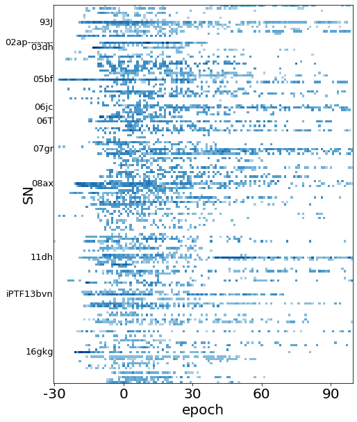
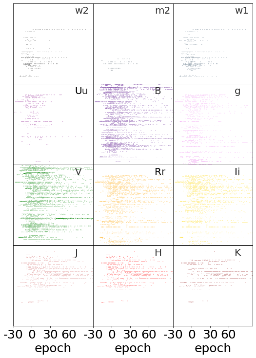
Figure 2: Left: Photometric coverage, in any band, for all 165 light curves in our sample, out to 100 days past peak. The name of SNe with more than 500 observations are explicitly indicated. As expected, most coverage is seen near peak, although a few light curves have consistently dense coverage throughout (e.g., SN 2007gr, SN 2011dh, SN 2006jc). Right: Photometric coverage for all 165 light curves in our sample in each of the considered photometric bands: ${w2,~{}m2,~{}w1,~{}U,~{}u,~{}B,~{}g,~{}V,~{}r,~{}R,~{}i,~{}I,~{}J,~{}H,~{}K_{s}}$, as labeled. $Uu$, $Rr$ and $Ii$ are plotted together. $B,V,Rr,Ii$ have the most coverage. The color bar reflects the mapping of color saturation to number for all subplots (illustratively shown in blue but consistent for all panels).

It is necessary to have a self-consistent definition and determination of the epoch of maximum to properly align the light curves when creating templates. Thus, in order to retain an object in our sample we require knowledge of the epoch of maximum brightness in $V$ band ($\mathrm{JD}_{\mathrm{max}}$), which we determine as described in B14 and section 4, either from the $V$ band itself, or from $B,~{}R/r^{\prime}$, or $I/i^{\prime}$ photometry. As an example, SN 2010S is removed from the sample because $\mathrm{JD}_{\mathrm{max}}$  cannot be determined in any of these bands.

We look for a primary peak in the light curve in $V$  $R/r^{\prime}$, $I/i^{\prime}$ or $B$. The epoch of maximum $\mathrm{JD}_{\mathrm{max}}$ and the observed peak brightness and their uncertainties are obtained through a Monte Carlo method as described in B14: a time region around maximum deemed by visual inspection suitable for fitting second-degree polynomial is chosen. Data in this region are re-sampled over the observed uncertainties and $n_{\mathrm{edge}}\leq 3$ data points at each edge of the chosen region are added with $n_{\mathrm{edge}}$ chosen by a stochastic draw for each realization. This bootstrapping method allows the determination of the epoch of maximum and its confidence interval.

For each band, if we do not have a direct measure of the $\mathrm{JD}_{\mathrm{max}}$ from the light curve in that band we derive it from the peak location in other bands, using peak offsets measured in B14 (Table 1, as calculated from the CfA data). To extend the procedure to bands not included in B14 ($g$ and UV bands ${w2,~{}m2,~{}w1}$), we fit the values in B14 table 1 as a function of the filter’s effective wavelength ($\lambda_{\mathrm{eff}}$ in $\AA$) with a second-degree polynomial, which gives us the equation:

$$\mathrm{Peak}_{V}-\mathrm{Peak}_{\lambda_{\mathrm{eff}}}[{\rm days}]= - 4.5_{-5.5}^{-3.4}\times 10^{-8}\lambda_{\mathrm{eff}}^{2}$$ (1)

$$+ 1.9^{2.2}_{1.6}\times 10^{-3}\lambda_{\mathrm{eff}}$$ (2)

$$- 9.5^{-8.2}_{-11}~{}[{\rm days}].$$ (3)

Note that this procedure leads to an interpolation for $g$ band, but an extrapolation in UV bands, with decreased reliability. subsubsection 3.1.3 contains the list of the SESNe in our sample along with their subtypes, time of $\mathrm{JD}_{\mathrm{max}}$, error in $\mathrm{JD}_{\mathrm{max}}$, and redshift.

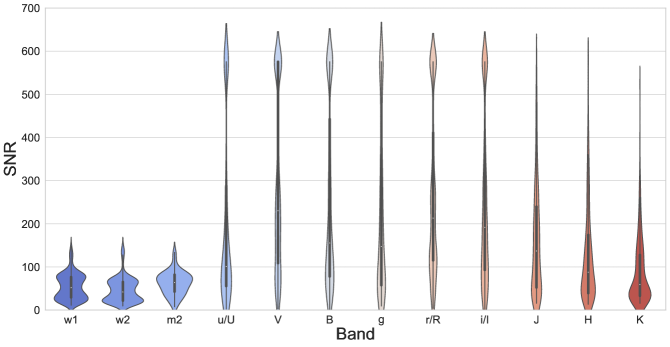
Figure 3: Distribution of the S/N of the photometry used in this analysis, different photometric bands shown along the $x$-axis. For each band, the S/N distribution is shown as a violin plot where the distribution is smoothed via Kernel Density Estimation and the median, inter-quartile-range (IQR), and full extent of the distribution are shown by a white dot, thick gray bar, and thin gray line respectively. While our photometric templates will be generated separately for each band, for the purpose of this plot the S/N measurements for $u^{\prime}/U$, $r^{\prime}/R$ and $i^{\prime}/I$ are considered together. As expected, optical bands, and in particular $V$, $B$, and $g$, have a higher median S/N (101, 230, 156, 148, 213, and 192 for $u^{\prime}/U$, $V$, $B$, $g$, $r^{\prime}/R$, and $i^{\prime}/I$ respectively) than NIR and UV bands (median S/N = 88, 60, 52, 42, 64 for $H$ and $K_{s}$, $w1$, $w2$, $m2$, and median S/N of 137 for $J$) with the upper IQRs stretching out to $\mathrm{\emph{{S/N}}}>400$ for optical photometry.

We removed all upper limits, along with extremely late or extremely early phases and only included photometric measurements over a time range of -20 days $\leq$ $\mathrm{JD}_{\mathrm{max}}$$\leq$ 100 days. For example, SN 2008D and SN 2002ap had measurements later than 3 years after $\mathrm{JD}_{\mathrm{max}}$, and OGLE targets typically have upper limit photometry available for one hundred days before the SN explosion. In Appendix B we summarize in three additional tables the photometric features of our sample including the number of photometry measurements for each SN, the first and last photometric epoch (in days from $\mathrm{JD}_{\mathrm{max}}$), and the mean and standard deviation of the photometric sample.

When we create the individual templates for each subtype (IIb, Ib, Ic, Ic-bl, and Ibn) we select from this sample the non-peculiar SNe of that sub-type and further reject light curves whose photometry does not lead to a good GP interpolation (as we will describe in section 5).

3.1.3 Final SESN sample

At the end of this process, we assembled a sample of 165 SNe for constructing SESN templates that include all SESN subtypes SNe IIb (34), SNe Ib (38), SNe Ic (33), SNe Ic-bl (25), SNe Ib (14), Ca-rich SNe Ib/Ic (3), peculiars (Ib-pec, Ic-pec, 5), Ib/c (14, including one SN IIb/Ib, one SN Ib/c-bl and one SN Ic/c-bl). Figure 2 shows the coverage in any band, and in each band separately, for our sample, limited to $-30\leq$$\mathrm{JD}_{\mathrm{max}}$$\leq 100$ days.

Table 1: Photometric Templates SESNe sample

Name	Type	Vmax	Vmax err	z
SN1954A	Ib	34850.3	3.6	0.001
SN1962L	Ib/c∗	38008.3	0.1	0.004
SN1983N	Ib	45529.4	2.6	0.003
SN1983V	Ic	45681.4	2.0	0.006
SN1984I	Ib	45847.8	0.6	0.011
SN1985F	Ib/c∗	45871.1	1.8	0.002
SN1991N	Ic	48349.0	2.0	0.003
SN1993J	IIb	49095.2	0.0	—–
SN1994I	Ic	49451.9	0.0	0.002
SN1996cb	IIb	50452.7	0.0	0.002
SN1997ef	Ic-bl	50793.2	0.3	0.012
SN1998bw	Ic-bl	50945.5	0.0	0.009
SN1999dn	Ib	51419.1	0.3	0.009
SN1999ex	Ib	51501.3	0.1	0.011
SN2001ig	IIb	52273.4	6.4	0.003
SN2002ap	Ic-bl	52314.5	0.1	0.002
SN2002ji	Ib	52620.9	1.4	0.005
SN2003bg	IIb	52721.0	1.3	0.005
SN2003dh	Ic-bl	52740.6	1.8	0.169
SN2003id	Ic-pec	52911.8	0.1	0.008
SN2003jd	Ic-bl	52943.3	0.6	0.019
SN2004aw	Ic	53091.5	0.7	0.016
SN2004dn	Ic	53231.1	0.3	0.013
SN2004dk	Ib	53243.9	1.9	0.005
SN2004ex	IIb	53308.4	0.3	0.018
SN2004ff	IIb	53314.9	1.5	0.023
SN2004fe	Ic	53319.3	0.5	0.018
SN2004ge	Ic	53335.6	1.6	0.016
SN2004gq	Ib	53363.0	1.9	0.006
SN2004gt	Ic	53363.1	0.2	0.005
SN2004gv	Ib	53367.4	0.2	0.020
SN2005az	Ic	53473.9	0.8	0.009
SN2005bf	Ib	53499.0	0.3	0.019
SN2005by	IIb∗	53504.0	2.4	0.027
SN2005fk	Ic-bl	53627.5	3.1	0.234
SN2005hl	Ib	53632.1	2.2	0.023
SN2005em	IIb∗	53648.6	0.4	0.025
SN2005hm	Ib	53652.0	2.0	0.035
SDSS-II SN 5339	Ib/c	53652.4	2.0	0.138
SDSS-II SN 4664	Ib/c	53673.4	2.8	—–
SDSS-II SN 6861	Ib/c?∗	53673.4	2.3	0.191
SDSS-II SN 8196	Ib/c	53680.5	3.3	0.080
SN2005hg	Ib	53684.4	0.3	0.021
SN2005kr	Ic-bl	53690.6	2.2	0.134
SN2005ks	Ic-bl∗	53691.5	1.4	0.099
SN2005kl	Ic	53703.7	0.6	0.003
SN2005kz	Ic	53712.9	0.4	0.027
SN2005mf	Ic	53734.6	0.1	0.027
SN2006T	IIb	53782.1	1.1	0.008
SN2006aj	Ic-bl	53794.7	0.6	0.033
SN2006ba	IIb∗	53825.7	1.7	0.019
SN2006bf	IIb	53826.5	1.3	0.024
SN2006cb	Ib	53861.5	1.6	0.026
SN2006el	IIb	53984.7	0.1	0.017
SN2006ep	Ib	53988.6	0.1	0.015
SN2006fo	Ib	54005.6	1.3	0.021
SN2006ir	Ib/c∗	54015.3	2.0	0.020
SN2006jo	Ib	54016.6	1.3	0.077
SDSS-II SN 14475	Ic-bl	54020.3	2.3	0.144
SN2006lc	Ib	54041.4	2.0	0.016
SN2006lv	Ib∗	54045.6	1.1	0.008
SN2006nx	Ic-bl∗	54056.1	2.0	0.125
SN2007C	Ib	54117.0	0.5	0.006
SN2007I	Ic-bl	54118.4	2.3	0.022
SN2007D	Ic-bl	54123.3	0.8	0.023
SN2007Y	Ib	54165.1	0.2	0.006
SN2007ag	Ib	54170.3	0.4	0.021
SN2007ay	IIb	54200.4	0.9	0.015
SN2007ce	Ic-bl	54226.7	2.0	0.046
SN2007cl	Ic	54250.9	1.0	0.022
SN2007gr	Ic	54339.3	0.3	0.002
SN2007ke	Ib-Ca	54367.6	1.9	0.017
SN2007kj	Ib	54382.5	0.1	0.018
SN2007ms	Ic/Ic-bl∗	54384.8	1.3	0.039
SDSS-II SN 19065	Ib/c	54393.7	2.7	0.154
SN2007nc	Ib	54397.0	1.3	0.087
SN2007qw	Ic∗	54412.8	1.3	0.151
SDSS-II SN 19190	Ib/c?∗	54414.0	5.3	—–
SN2007qv	Ic	54415.6	2.7	0.094
SN2007ru	Ic-bl	54440.5	0.3	0.016
SN2007rz	Ic	54456.5	3.1	0.013
SN2007uy	Ib-pec	54481.8	0.7	0.007
SN2008D	Ib	54494.7	0.1	0.007
SN2008aq	IIb	54532.7	0.5	0.008
SN2008ax	IIb	54549.9	0.1	0.002
SN2008bo	IIb	54569.7	0.2	0.005
SN2008cw	IIb	54620.8	1.5	0.032
SN2009K	IIb∗	54869.6	1.7	0.012
SN2009bb	Ic-bl	54923.6	0.1	0.010
SN2009er	Ib-pec	54982.6	0.2	0.035
SN2009iz	Ib	55109.4	1.4	0.014
SN2009jf	Ib	55122.2	0.1	0.008
SN2009mg	IIb	55189.5	0.0	0.008
SN2009mk	IIb	55193.2	0.3	0.005
SN2010X	Ic?∗	55238.8	1.3	0.015
SN2010ay	Ic-bl	55270.2	1.4	0.067
SN2010bh	Ic-bl	55282.1	0.2	0.059
SN2010al	Ibn	55283.9	0.7	0.017
SN2010as	IIb∗	55289.6	2.0	0.007
SN2010cn	IIb/Ib∗	55331.4	0.4	0.026
SN2010et	Ib-Ca∗	55358.7	2.2	0.023
PTF10qts	Ic-bl	55428.2	0.4	0.091
SN2010jr	IIb∗	55531.7	1.0	0.012
SN2011am	Ib	55636.5	0.6	0.007
SN2011bm	Ic	55679.2	1.6	0.022
SN2011dh	IIb	55733.1	0.2	0.002
SN2011ei	IIb	55787.2	0.0	0.009
PTF11kmb	Ib-Ca∗	55799.7	1.3	0.017
PTF11qcj	Ic-bl∗	55842.3	2.2	0.028
SN2011fu	IIb	55847.5	0.1	0.018
SN2011hg	IIb	55878.9	0.6	0.024
SN2011hs	IIb	55889.2	0.3	0.006
SN2011hw	Ibn	55904.7	2.0	0.023
SN2012P	IIb∗	55951.9	2.3	0.005
SN2012ap	Ic-bl	55976.6	0.5	0.012
PS1-12sk	Ibn	56003.7	1.7	0.054
SN2012au	Ib	56007.3	1.0	0.005
SN2012hn	Ic-pec	56032.9	0.5	0.008
SN2012cd	IIb	56034.6	1.7	0.012
SN2012bz	Ic-bl	56055.8	1.5	0.283
PTF12gzk	Ic-pec	56149.9	0.8	0.014
PTF12hni	Ic	56170.7	2.6	0.106
OGLE-2012-sn-006	Ibn	56215.9	1.5	0.060
SN2013ak	IIb	56369.1	0.2	0.004
SN2013cu	II	56424.4	1.2	0.025
SN2013cq	Ic-bl	56433.5	1.5	0.339
SN2013df	IIb	56470.0	0.2	0.002
iPTF13bvn	Ib	56476.3	0.4	0.004
SN2013dk	Ic	56476.5	0.2	0.005
LSQ13ccw	Ibn	56539.0	1.2	0.060
OGLE-2013-SN-091	Ic	56578.0	2.5	0.080
OGLE-2013-SN-134	Ic	56578.0	2.5	0.039
SN2013ge	Ic	56621.4	0.2	0.004
SN2014C	Ib	56671.2	0.1	0.003
SN2014L	Ic	56695.7	0.1	0.008
OGLE-2014-SN-014	Ib	56697.4	2.4	0.043
SN2014ad	Ic-bl	56741.3	0.2	0.006
LSQ14efd	Ib∗	56900.0	0.6	0.080
OGLE-2014-SN-131	Ibn	56969.1	2.6	0.085
ASASSN-14ms	Ib	57024.0	0.8	0.065
SN2015U	Ibn	57071.4	0.2	0.014
OGLE15eo	Ic	57263.7	2.0	0.064
SN2015ap	Ib/c-bl	57287.4	0.5	0.011
OGLE15jy	Ib/c?	57298.1	2.0	0.060
iPTF15dld	Ibn∗	57308.0	1.9	0.047
OGLE15rb	Ic	57341.0	1.6	0.028
iPTF15dtg	Ic	57353.9	2.0	0.052
OGLE15vk	Ic	57357.4	1.7	0.050
SN2016bau	Ib	57478.8	1.3	0.004
DES16S1kt	IIb	57641.7	2.2	0.069
SN2016gkg	IIb	57678.7	5.5	0.005
OGLE16ekf	IIb	57680.0	1.0	0.068
SN2016hgs	Ib	57690.9	2.0	0.017
SN2017ein	Ic	57914.6	1.9	0.003
SN2018bcc	Ibn	58232.4	2.0	0.064
SN2019bjv	Ic	58530.6	1.5	0.027
SN2019all	Ib/c	58538.1	1.7	0.037
SN2019gqd	Ic	58646.5	1.5	0.036
SN2019ilo	Ic	58679.2	2.3	0.034
SN2019pik	Ic	58734.9	1.6	0.118
SN2019myn	Ibn	58706.0	2.3	0.100
SN2019php	Ibn	58730.3	1.3	0.087
SN2019rii	Ibn	58755.9	1.6	0.123
SN2019aajs	Ibn	58540.9	2.2	0.036
SN2019deh	Ibn	58587.1	2.4	0.055

Note. — Classification of SESNe denoted with ^∗ are modified by us after running SNID with the largest SESN template database on their spectra close to maximum light.

Figure 3 shows the distribution of the signal-to-noise ratio (S/N) of the photometry in our sample in different bands (where the S/N is the ratio of flux to flux error as derived from the magnitudes). Some extremely high S/N measurements are available, especially in the optical bands where the distribution of S/N appears bimodal, with the median $\mathrm{\emph{{S/N}}}_{u/U}\sim 100$ in $u/U$ band, and median $\mathrm{\emph{{S/N}}}_{V,~{}r/R}>200$ in $V$ and $r/R$ bands, and a secondary distribution peak $500\leq\mathrm{\emph{{S/N}}}\leq 600$ in all optical bands, while, as expected, we see that the NIR bands have lower S/N compared to the optical bands with median $50\leq\mathrm{\emph{{S/N}}}_{{J,~{}H,~{}K_{s}}}\leq 100$ and lower yet in the UV bands (median $\mathrm{\emph{{S/N}}}_{{w2,~{}m2,~{}w1}}<150$). Our photometric sample has diverse sampling, diverse noise, and generally a smooth behavior, with greater diversity at early times, compared to later phases (after the ⁵⁶Ni decay starts dominating). Three examples of time series in our sample are shown in Figure 4.

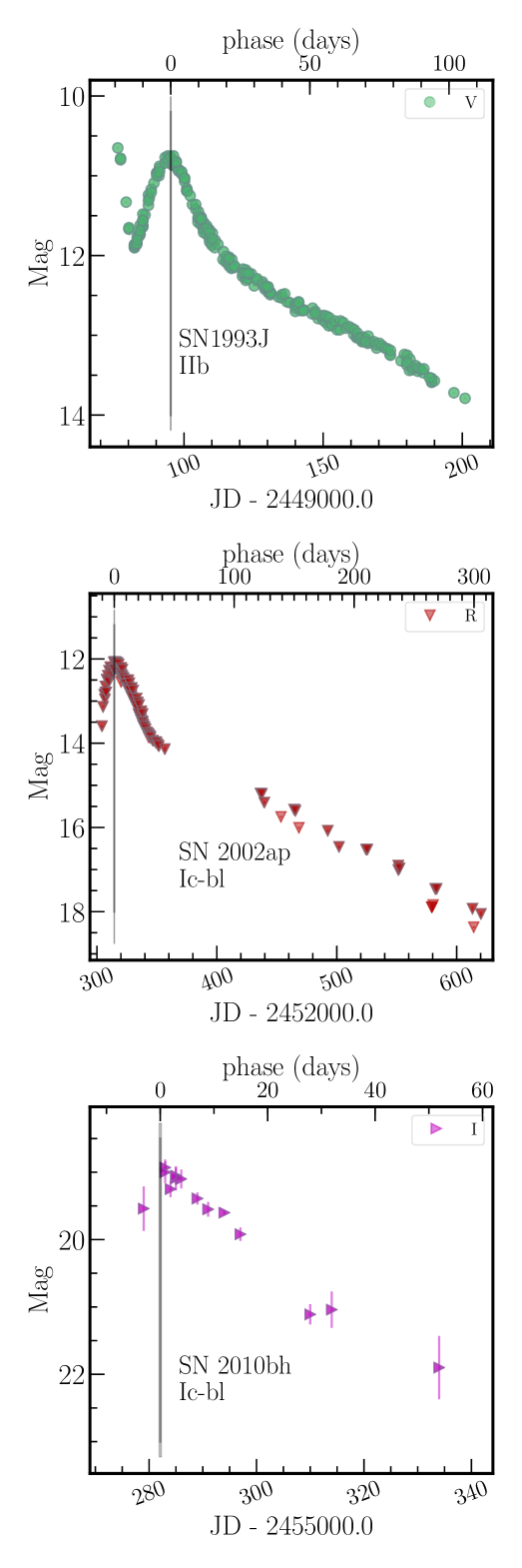
Figure 4: Examples of SN light curves, from heterogeneous photometric sources. For each SN the date of V band maximum $\mathrm{JD}_{\mathrm{max}}$ is marked by a vertical black line, and its $1\sigma$ uncertainty is marked as a gray region (to enhance visibility, since the uncertainty is typically very small, the $1\sigma$ uncertainty region extends further above and below the $\mathrm{JD}_{\mathrm{max}}$ line). SN 1993J $V$-band (top) is very well-sampled, possibly with underestimated uncertainties. SN 2002ap $R$-band (center) is well-sampled around the peak but it shows large gaps later. SN 2010bh $I$-band is a sparsely sampled light curve with uncertainties conveying the scatter properly (bottom). Many publications are dedicated to each of these supernovae: for SN 1993J the first articles appeared in 1993, Okyudo et al. 1993, and the most recent at the time of writing is Zsíros et al. 2022. For SN 2002ap Gal-Yam et al. 2002 and recent modeling work include Zapartas et al. 2017. For SN 2010bh see work including Fan et al. 2011 and Bufano et al. 2012.

3.2 Photometric corrections

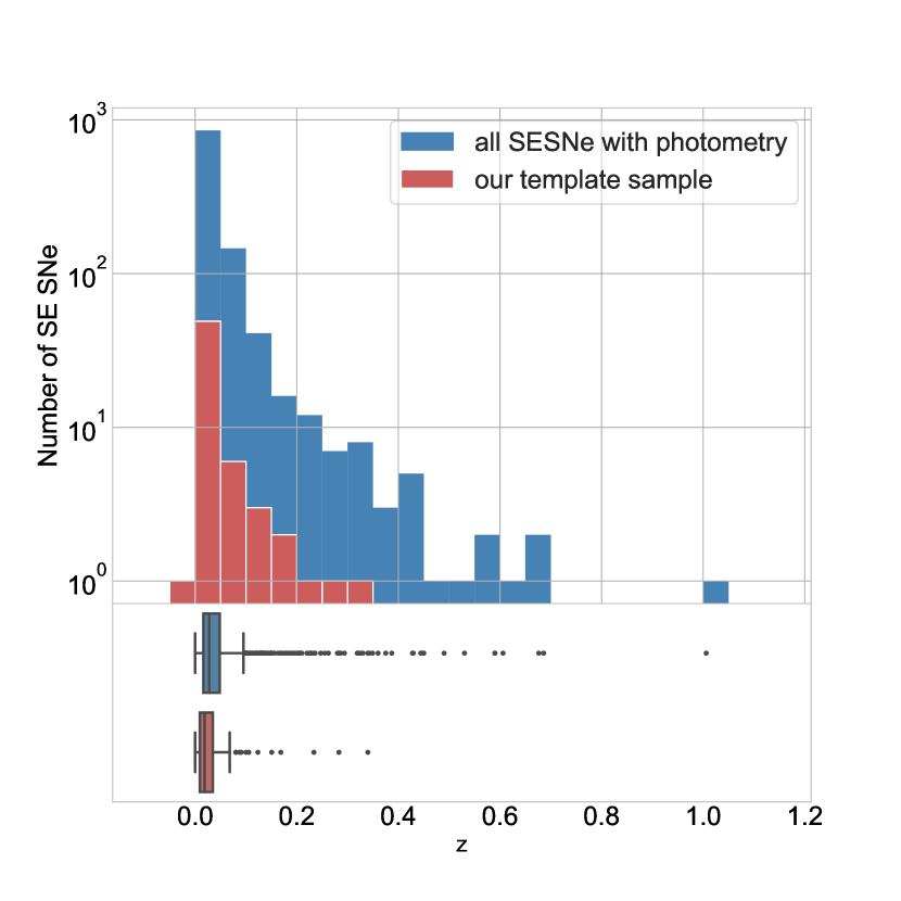
Figure 5: Redshift $z$ distribution for all SESNe in the literature, as collected by the Open SN Catalog (OSNC), and for the subsample we will use for template construction. Top: a histogram of the distributions in 10 bins. Bottom: box and whiskers plot of the distributions. A box and whiskers plot shows the median of the distribution as a vertical line, the 25-th percentiles as a colored box (i.e: the inter-quartile range, IQR), and the bars, joined to each end of the box by a line, represent the minimum and maximum of the distribution excluding statistical outliers, where outliers are defined as any point farther than 1.5$\times$IQR from the edges for the IQR. The “outliers” thus defined are shown as data points. None of the SNe in the full literature sample exceeding $z=0.4$ is in the selected “well-observed” sample which is used for template construction. At a $z=0.4$ the spectra are shifted by the typical width of an optical photometry band, so that the $r^{\prime}$ rest-band, for example, would be observed in the $i^{\prime}$ filter. The template sample has a median of 0.017 and a 99.7 percentile (equivalent to a $3-\sigma$ in a Gaussian distribution) of 0.31. Notice that the low-$z$ edge of the distribution is below zero: SN 1993J and SN 2004gk, extremely near-by objects, have negative recession velocities ($z~{}=~{}-1.13\times 10^{-4}$ and $z~{}=~{}-5.50\times 10^{-4}$ respectively.)

We do not apply any $k-$correction to the data, because the vast majority of the well-observed SESNe are in the local Universe. We show the redshift $z$ distribution for the complete SESNe sample of literature data from the OSNC and of the ultimate selection of SN that we will use to construct templates in Figure 5, as a histogram in 10 bins in the top panel, and as a box-and-whiskers plot in the bottom panel. The 16-th, 50-th (median), and 84-th percentiles of the $z$ distribution are 0.01, 0.02, 0.08 and 0.00, 0.02, 0.06 for the full sample and the subsample selected for photometry (described in subsection 3.1) respectively, requiring a median wavelength shift $<=3\%$ in the SED for our sample. There are no SNe in our template subsample that exceeds $z=0.4$, which is the redshift value at which a spectrum is shifted by roughly a full optical band. Only three SNe exceed $z=0.2$: SN 2012bz (Schulze et al., 2014), and SN 2013cq (Melandri et al., 2014), both SNe Ic-bl connected with GRBs and first discovered in the $\gamma$-rays, and SN 2005fk (SN Ic-bl). $k$-correction requires an understanding of the full spectral evolution, including the effects of reddening, in order to interpolate between bands. The reddening in particular is extremely uncertain due to the intrinsic diversity of SESNe and to the difficulties in determining the reddening for objects that are not standardizable. So in order to not introduce additional errors, we refrain from applying $k$-corrections.

4 Combined SN Ibc Templates

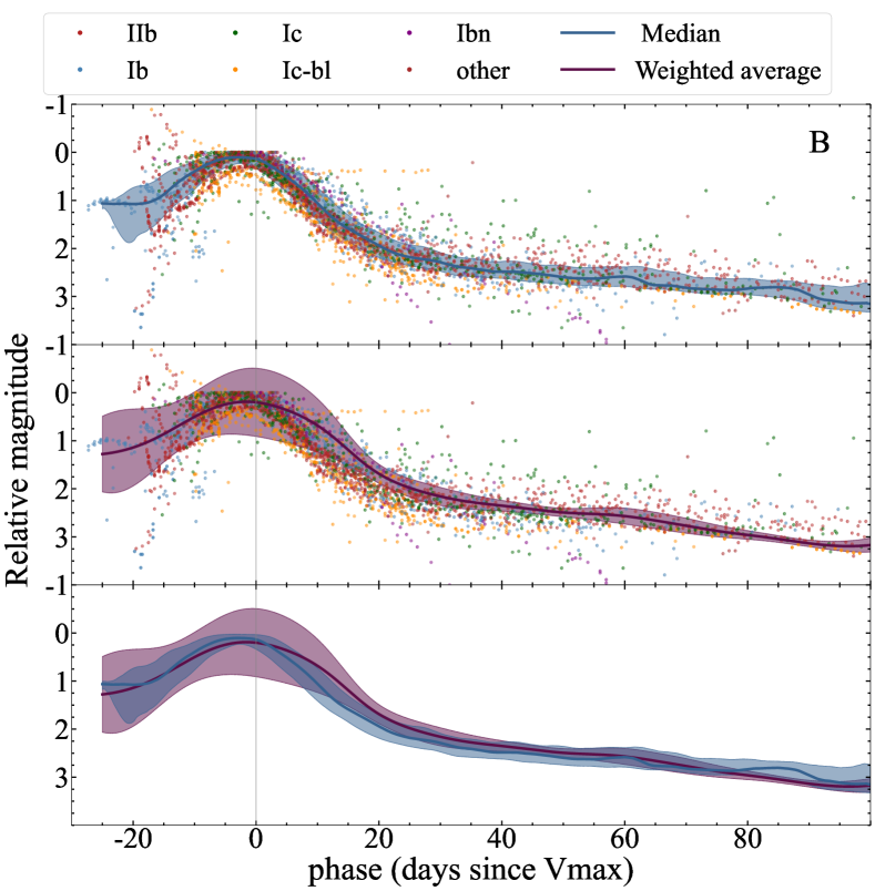
Figure 6: Top panel: The B-band median template for all SESNe generated as described in section 4 is shown as a blue line along with the IQR (shaded region). Datapoints for all light curves used in the generation of the template are shown, labeled and colored by SESN subtype. Middle panel: Same as the top panel for the weighted-average templates and their weighted standard deviation uncertainty region (IQR). Bottom panel: The median template (blue line) and the weighted-average template (purple line) are shown together to aid comparison, along with their respective uncertainty as shaded red and grey areas respectively. The weighted-average template has larger uncertainties and is typically brighter due to a photometric bias introduced by the use of the photometric uncertainty to weigh the data points. We ultimately select the rolling median procedure to generate SN Ibc templates.

We begin by creating a preliminary template for all SESNe in each band, without differentiating by subtype. Following the literature, we call these templates “SN Ibc templates”. We wish to emphasize that this is a diverse class of transients. If we can identify distinct photometric behaviors, lumping all of them in one class will have a negative impact on our ability to classify transients photometrically. This is further addressed in subsection 5.5. However, we need to create SN Ibc templates to represent the average time-dependent behavior of SESNe in each of the bands to then subtract this template from the individual SN light curves and enable the GP fits (refer to section 5).

The construction of SN Ibc templates as a mean or median of the photometric measurements is a relatively standard procedure, done first in  Drout et al. (2011) and later in  Taddia et al. (2018) (both of these templates will be compared with ours in subsection 4.1). We now can do this in optical and NIR bands where we have several light curves, amounting to many data points for phases between -20 and 100 days.

First, we align the light curves in each band by their date of maximum brightness, with care to ensure we are indeed looking at the maximum brightness due to nucleosynthesis processes (rather than peaks that may occur due, for example, to shock breakout or interaction with interstellar material).

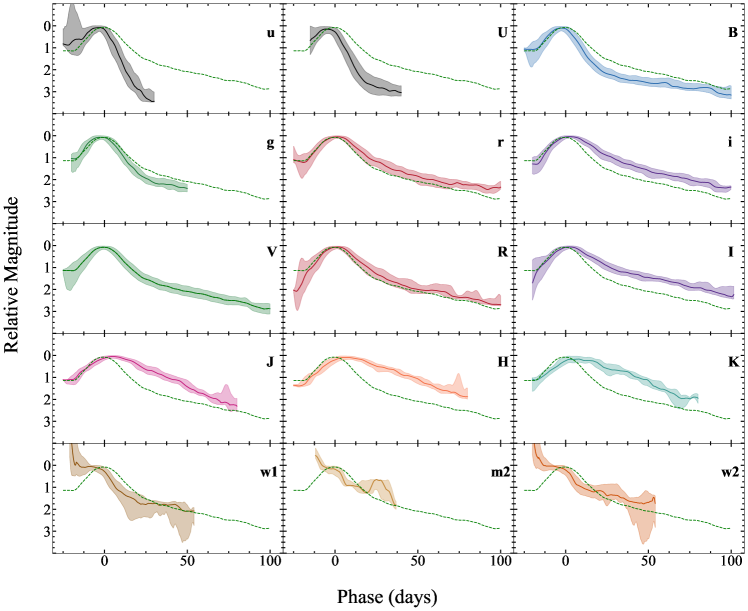
Figure 7: The data-driven SN Ibc templates produced as a rolling median of all photometric data points available in each band as described in section 4. The number of SNe used to construct each template is: $U$: 39, $u$: 20, $B$: 75, $V$: 80, $R$: 41, $r$: 57, $I$: 27, $i$: 55, $J$: 23, $H$: 22, $K_{s}$: 18, $w1$: 15, $w2$: 15, and $m2$: 9. The SN Ibc median template and its IQR is shown in each band as a solid line and shaded region. For reference, the $V$ band template is plotted in each panel (as a green dashed line).

Next, with the light curves now in phase space with peak brightness corresponding to phase = 0, we scale the observed magnitude by setting to 0 the magnitude of the brightest data point between phases -5 and 5 days. We remove light curves that have no data points in that range. Scaling the light curves’ brightness to an observed data point, rather than to the maximum found by fitting a smooth interpolation to the data, adds some scatter in the templates’ photometry but it prevents us from making model-driven assumptions. The additional scatter generated by small misalignments, in fact, makes our estimate of the template uncertainties conservative. However, in the presence of shock breakout or cooling envelope signatures, the brightest point near $\mathrm{JD}_{\mathrm{max}}$ may not be associated with the ⁵⁶Ni-driven evolution of the SN, thus we reject these final adjustments where the visual inspection suggests the presence of such contamination, and scale those light curves to $m($$\mathrm{JD}_{\mathrm{max}}$$)=0$. The light curve of SN2013df (SN IIb) in the $R$ band is an example of such contamination.

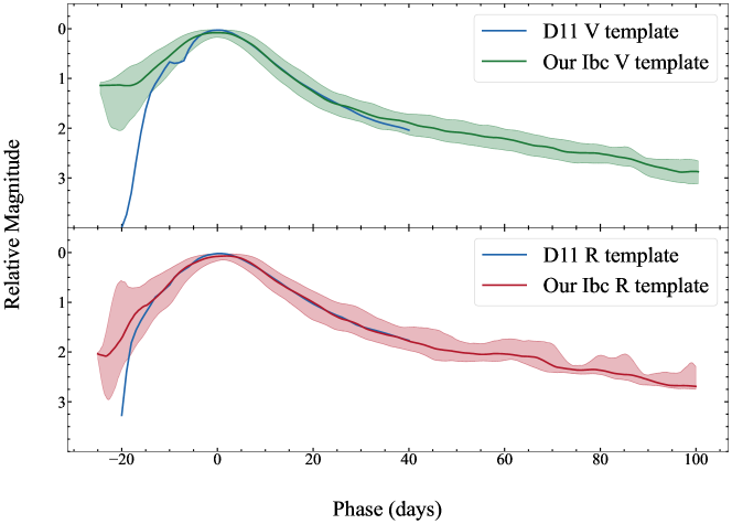
Figure 8: Comparison of our templates with the templates published in D11. Our SN Ibc templates are plotted as a solid line in color and the D11 templates are plotted as a solid blue line. D11’s SESNe templates are available for $V$ and $R$ band https://www.cfa.harvard.edu/~mdrout/data/V_template.txt and https://www.cfa.harvard.edu/~mdrout/data/R_template.txt, accessed on February 12th, 2021. D11’s photometry suffers from galaxy contamination (see B14) but the templates are mostly based on well-sampled literature light curves and therefore the contamination is likely not significant. The post maximum light curve decay is consistent with what we measure, however, the light curve rise is far steeper for D11. Notice that the uncertainty on D11’s templates, plotted in their figures 2, 3, and 5 of D11, is not reproduced in our figure since it is not available online. Nonetheless, since this uncertainty simply represents the standard deviation of the sample and the early time the template behavior is based on 1-to-a few light curves, the uncertainty as plotted in D11 goes to 0 in the earliest epochs and does not help reconcile the pre-maximum discrepancy between our template and D11 templates.

Figure 9: Comparison of our templates with the templates published in T15 for the common bands $u^{\prime},~{}r^{\prime},~{}i^{\prime}$, accessed at Vizier catalog J/A+A/574/A60/template on February 12th, 2021. The rise portion of the templates, which was the focus of T15, is steeper than our rise, and the decay is slightly shallower in all bands. In $u^{\prime}$ and $i^{\prime}$, T15 templates seem to have weak signatures of shock-breakout, but they seem to be dimmer than the lower range of the uncertainties of our templates.

We can now proceed to aggregate the light curves into templates. We produced templates with two different methods: First, we create a smoothed, rolling weighted-average template. In order to account for the heteroscedastic nature of the photometric measurement uncertainties, especially when observing a diverse sample of SNe with diverse brightness characteristics and with different instrumentation, we use, as customary, averages weighted by the inverse of the squared uncertainty of each measurement.

Second, compute a smoothed, rolling median template, with a 5-day rolling window. This rolling median is noisy, getting noisier at late and early times where fewer SNe are observed, with the IQR artificially shrinking where the number of SNe in the window drops to only a few. The rolling median template is then smoothed using the Savitzy-Golay filter (Press & Teukolsky, 1990) (see details below).

Figure 6 shows a comparison of the median and weighted-average templates for band $B$. The weighted average template tends to be brighter than the median template. This effect is even more extreme in other bands. This is simply because of an observational bias: the brighter data points generally have larger weights (smaller uncertainties). While the SNe themselves have a range of brightness and are observed by systems with different accuracy, in the aggregate, the slow-evolving light curves have smaller uncertainty in the late measurements which causes them to dominate the late time average templates, introducing a bias. For this reason, we use the smoothed rolling median as SN Ibc templates for the rest of the analysis.

Our final SN Ibc templates are shown for each band in Figure 7 as a gray line, with the IQR shown as a pale-filled region. The steps taken to generate these SN Ibc templates are as follows:

• Phases are defined as an array between -20 and 100 with 24 points within each day for each hour.

• At each hour, data points from all of the selected SNe between that hour and its next five days are selected.

• The medians and IQRs are calculated within each 5-day window.

• The median is then smoothed using a Savitzy-Golay filter within windows of 171 data points using a third-degree polynomial.

In some bands, towards the beginning and end of the light curves where data is sparse, the rolling median shows sudden jumps that could not be smoothed by our procedure. To avoid these undesirable features we restrict the range of phases over which we produce the templates to whatever is appropriate in that band. These phase boundaries are shown in Table 2 for each band. The data is insufficient to produce effective and accurate templates in the ultraviolet bands. The $w1,w2$, and $m2$ templates are included for completeness, but we caution the reader that these templates are produced from small datasets (see Figure 7).

Table 2: Phase Range for Ibc templates in each band.

Band	Phase Range	Band	Phase Range
	(days)		(days)
u	-25,30
U	-15,40	w2	-20,50
B	-25,100	m2	-20,40
g	-20,50	w1	-20,50
V	-25,100
r	-25,100	J	-25,100
R	-25,100	H	-25,100
i	-20,100	K	-25,100
I	-20,100

4.1 Comparison of the Ibc templates

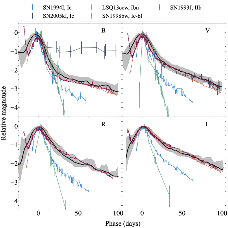
Figure 10: The SN Ibc templates made of all photometric data points available for all SESNe subtypes (black curves) in each of the bands $B$, $V$, $R$, $I$. These templates are plotted along with light curves of those SNe that have been claimed as prototypical of their class. For example, SN1994I and SN2005kl have been claimed to be prototypical SN Ic, but clearly deviate from our template.

In Figure 7 we show our SESN Ibc templates for all the available photometric bands: ${w2,~{}m2,~{}w1,~{}U,~{}u,~{}B,~{}g,~{}V,~{}r,~{}R,~{}i,~{}I,~{}J,~{}H,~{}K_{s}}$. Although we do calculate and plot the templates for UV Swift ${w2,~{}m2,~{}w1}$ bands, the sparsity and low S/N of the data in these bands only allow us to generate very noisy templates, which we show for completeness. The error bands represent the epoch-by-epoch IQR, and the SN Ibc template in $V$ band is plotted for reference, as a dashed green line in each panel. We can immediately notice that the light curves decline faster in bluer bands. We quantify the rise and decline rate of the templates with the parameters $\Delta m_{-10}$ and $\Delta m_{15}$. $\Delta m_{15}$ was first introduced by Phillips (1993) to measure the evolutionary rate of SNe Ia (leading to their standardization). This parameter measures the magnitude change from $\mathrm{JD}_{\mathrm{max}}$ to ${\rm phase}=\mathrm{JD}_{\mathrm{max}}+15$ days, and $\Delta m_{-10}$, similarly, measures the rate of change between ${\rm phase}=\mathrm{JD}_{\mathrm{max}}-10$ days and $\mathrm{JD}_{\mathrm{max}}$. The measured $\Delta m$’s for our SN Ibc templates are shown in LABEL:tab:del_m15 and LABEL:tab:del_m10. The uncertainty on these quantities (also reported in LABEL:tab:del_m15 and LABEL:tab:del_m10) is simply the $\Delta m$ measured at the edge of the template’s IQR.

Next, we compare our SN Ibc template with SN Ibc templates previously released in the literature. The comparison with  Drout et al. (2011) for $V$ and $R$ bands, shown in Figure 8. The light curve decline is consistent in both bands with our SN Ibc templates within the IQR. However, the early light curve behavior, the hardest to model typically due to the rarity of SESN observations in the early phases of evolution, differs significantly, especially in the $V$ band. In addition, the uncertainty in the D11 templates artificially shrinks at early epochs, due to sparse observations. Meanwhile, in our templates, the intrinsic diversity in behavior at early times is properly represented by the growing uncertainty. Early bumps in light curves are explained by shock-breakout (for SNe Ic-bl) and shock cooling (see for example Filippenko et al., 1993; Ciabattari et al., 2011, 2013, and discussion in subsection 5.8). Since 2011 several SESN light curves have been observed to show such features. These SNe contribute to lifting our template at early times, especially in bluer bands.

T15 also released Ibc templates, obtained as a 12th-degree polynomial fit to the $z<0.1$ SESNe in the SDSS sample. In Figure 9, we show how they compare to our templates. T15’s templates have a slightly shallower fall (slower decay) than our rolling-median templates, while the rise is significantly faster than we measure.

Comparing our SN Ibc templates generated with a larger, yet heterogeneous sample of SESNe and a more statistically sophisticated method for data aggregation than previous work, with D11 and T15, we find that:

• The new SN Ibc templates include a measure of the uncertainty, previously missing.

• Adding more SNe to the sample allows us to extend the templates to earlier and later epochs compared to D11 and T15.

• The new SN Ibc templates are generated for additional bands.

• While the new templates do not dramatically change our understanding of the time evolution of SN Ibc in any band for which templates previously existed ($V$, $R$, $u$, $r$, and $i$ bands), differences arise with significance above the IQR at early and late epochs.

4.1.1 Photometrically prototypical and unusual SN Ibc’s

Below we discuss a few SESNe that stand out as prototypical and a-typical in comparison with our SN Ibc templates in $B$, $V$, $R$, and $I$ bands. These objects are shown in Figure 10.

SN 1994I, often considered a prototypical SN Ic, has narrow light curves rising and declining by one magnitude around the peak in less than 10 days. We suggest that SN1994I should never be regarded as a typical SN Ic, since is neither a spectroscopically typical SN Ic (see M14), nor a photometrically typical SESN, as shown here.

LSQ13ccw stands out compared with the SN Ibc template as it has a narrow light curve, with a fast rise and a fast decline.

SN 2005kl shows a plateau in its $B$ band light curve but shows normal behavior in $V$.

We have also plotted the light curves of SN 1998bw and SN 1993J(Figure 10), which are known as prototypical SNe Ic-bl and SNe IIb respectively to show that these light curves are overall well fit by our SN Ibc templates within the IQR and can indeed be considered photometrically prototypical SNe Ibc.

5 GP Templates

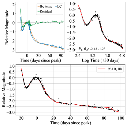
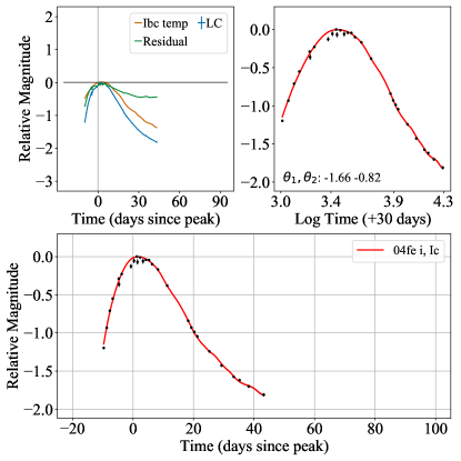
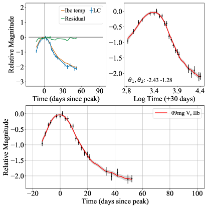
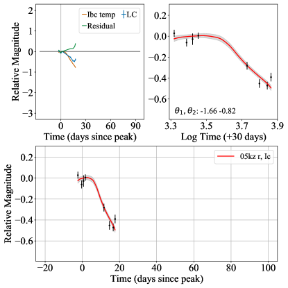
Figure 11: From top left and moving clockwise: SN1993J $B$ band, SN2004fe $i$ band, SN2009mg $V$ band, and SN2005kz $r$ band. For each plot, the top left panel includes the time series, SN Ibc template for that band, and the residual between the two, and the right panel shows the light curve along with its GP fit in the logarithmic time domain where the fit is performed. The bottom panel is the fit in natural time. The red line is the mean of the fit and the gray band (occasionally too thin to see) represents the uncertainty (point-by-point standard deviation of the GP realizations). To learn more about SN 2009mg see Oates et al. 2012.

We want to generate templates for each SN subtype, IIb, Ib, Ic, Ic-bl, and Ibn, so we need a more sophisticated scheme than simply averaging over all SN photometry since the data per band per SN subtype is generally scarce and sparse. We want an interpolation procedure that:

1. Captures the diversity in the SN sample: Using a non-parametric model allows us to capture any peculiar behavior. We fit the light curves with Gaussian Processes (GP) using the george Python module.

2. Captures the early time variability, and the late time smoothness: Since variability is expected to be larger at early times, we fit the time in the logarithmic time domain.

3. Fits the observed data points : The goodness of fit is measured with a $\chi^{2}$ term in the objective function and is minimized to choose the hyperparameters of the GP.

4. Maintain smoothness: With the choice of a squared exponential kernel for the GP, which is infinitely differentiable, a smoothness requirement is implicitly enforced. However, non-discontinuous sharp features are still possible and not desirable, since we always observe SNe to be smooth on short time scales. An additional smoothness requirement is enforced by modifying the GP objective function adding a regularization term that minimizes the second derivative.

Despite being a rather old and established technique in many domains, first conceived by Daniel Krieg, a South African statistician in 1951 in the context of geospatial statistics (Krige, 1951), only recently GP have gained increasing traction in astronomy as a tool for data-driven Bayesian interpolation and modeling (e.g. Thornton et al. 2024, Boone 2019, Ambikasaran et al. 2014, McAllister et al. 2017, Pruzhinskaya et al. 2019, Qu & Sako 2021). For a review of GP applications in astronomy see Aigrain & Foreman-Mackey (2023). GPs are ideal in the creation of SN templates and have been used in Reese et al. (2015) to construct templates for SNe Ia and Vincenzi et al. (2019) to create single-object spectrophotometric templates of CC SNe. Reese et al. (2015) used a training set of 1500 SNe Ia and 7000 CC SNe. However, the fraction of stripped SNe in the CC sample is very small (15 objects) thus the parameter choice is not optimized for these subtypes. Vincenzi et al. (2019) fitted SNe individually to produce object-level models. We will build on these results with one important difference: GP interpolation is generated in log-time (point 2 above).

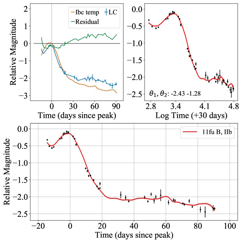
Figure 12: Panels and colors as in Figure 11, GP fit to Type IIb SN2011fu, $B$. Our model captures well the small excesses at early times which is a known characteristic of many SNe IIb (see for example Bersten et al., 2018; Arcavi, 2017; Orellana & Bersten, 2022), associated with a shock cooling component. However, the late fit shows high confidence features on days time scales that are likely unphysical (see phase $\sim{60}$ days) To learn more about SN 2011fu see Kumar et al. 2013 and Morales-Garoffolo et al. 2015a.

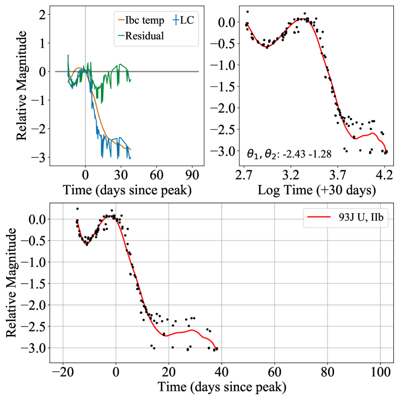
Figure 13: SN 1993J $U$: Color and panels are as in Figure 11. The small uncertainty in the data causes overfit with any choice of parameters that leads to the late time bump at $\sim 30$ (which is most apparent in the log fit top panel). Inflating the error bars by a factor $\sim 10$ gives a more realistic fit at late times at the cost of losing details at early times (including the cooling envelope-related early excess).

Because at this stage we are interested in comparing the photometric behavior in different bands, we are applying GP only on the temporal axis, while recent work has applied it in the two-dimensional space of time and wavelength.

To improve the stability of the GP fit, we subtract the SN Ibc templates (section 4) in each band from each SN and fit the residuals. We choose a square exponential kernel (ExpSquaredKernel in george)

$$k(d)=\theta_{1}^{2}\exp(\frac{-d^{2}}{\theta_{2}^{2}}).$$ (4)

To choose the best values of the model’s hyperparameters, $\theta_{1}^{2}$ and $\theta_{2}^{2}$ and $s$, we minimize the objective function: $\chi^{2}(m(t|\theta_{1}^{2},\theta_{2}^{2}))~{}+~{}{\sum_{t}{\left|\frac{d^{2}m(t|\theta_{1}^{2},\theta_{2}^{2})}{dt^{2}}\right|}}^{s},$ where $m$ is the GP-predicted magnitude and the second term is the second derivative of the predicted magnitude to a power of $s$ (points 3 and 4). $s$ determines the importance of the term that ensures a smoother fit in the objective function. Setting $s=1$ leads to good fits for most light curves except particularly fast-evolving light curves that have a narrow peak and fast magnitude variation in early phases. For fast-evolving SNe only (subsection 5.8) we choose $s=0.25$.

The hyperparameters $\theta_{1}$ and $\theta_{2}$ are first optimized for each SN in the sample independently. A subset of light curves that shows a good fit for phases between $-20$ and 20 is identified by visual inspection (110 SNe). Within this subset, for each SESNe subtype, we take the median of $\theta_{1}$ and $\theta_{2}$ as the chosen hyperparameter values. These values are reported in Table 3. Next, the SESNe of types IIb, Ib, Ic, Ic-bl, and Ibn are fit again with their subtypes’ hyperparameters. The fits are again visually inspected, and some light curves with bad fits are removed from the sample (read subsection 5.2). The final selected fits will be used to create the GP templates as explained in subsection 5.3.

Table 3: Selected kernel parameters for each subtype

	$\theta_{1}^{2}$	$\theta_{2}^{2}$
Ib	5.95	1.02
IIb	5.90	1.64
Ic	2.76	0.67
Ic-bl	1.39	1.99
Ibn	0.004	8.70

5.1 Successful fits

Generally, the fits capture well the time behavior of the single band light curves. Figure 11 shows a few examples of good fits. For each SN we show in the top panel the original observations, the SN Ibc templates, and the residuals between the two, which is what we actually fit with the GP procedure. On the right panel, we show the result of the GP in the logarithmic time domain. In the bottom panel, we show the final fit in natural time and the uncertainty bands generated by the GPs. In general, the uncertainty is very small for well-sampled light curves. Below are a few successful fits for SNe with extremely good sampling (SN 93J, $I$ band), with good sampling (05mf, $R$), and more sparse and noisy data (05mf, $H$). Features like small upturns of the light curves at early time are well fit by our method, as, for example, SN 2011fu in (Figure 12).

5.2 Bad fit and pathological cases

We identify three kinds of undesirable behaviors in the GP fits obtained through the procedure outlined above.

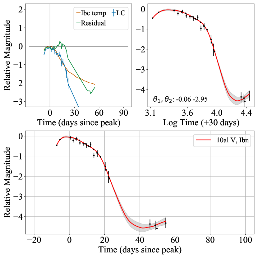
Figure 14: SN 2010al $V$: Color and panels are as in Figure 11. The light curve sampling ends before 60 days and the GP fit shows an upturn towards the end which is an artifact of the fit and not a feature of the supernova photometry.

5.2.1 Late time behavior

An upturn is seen in a few ($\sim 4$) light curves at the last few data points (e.g., in Figure 13 and Figure 14). Generally, these epochs are outside of the range where we create our templates.

As in the 2010al $V$ example, the GPs propagate the light curve continuing the latest trend in the data. If there are missing data points, the GP extrapolation will generate a light curve with an increasing trend in brightness in later epochs. This is a problem with the data, not with the GPs, that cannot be solved in a non-parametric fashion, without imposing strict constraints on the sign of the derivative, but that in return may not allow us to characterize individual peculiarities in SN light curve behavior.

5.2.2 Unphysical short-term variability

Some of the fits exhibit unphysical features at the regions with no or very few data points. In these regions, the GPs tend to converge to the mean of the distribution which in this case is the SN Ibc template, and the same features in the SN Ibc templates are projected into the GP fits. For instance, in Figure 12, there are only two data points around epoch 60 in the bottom panel where the fit exhibits some bump. If we look at the same interval for the SN Ibc template (orange curve in the upper left panel), we see the same features.

5.2.3 Bad fits

In some cases, the GP fit overall is not acceptable. In some bands like ultraviolet bands, this is due to a lack of data, large uncertainties, and a noisy SN Ibc template, and in other bands, due to having no data points between epochs $-5\leq\mathrm{JD}_{\mathrm{max}}\leq 5$ days. These fits are removed by visual inspection and not included in the GP template creation. 56 light curves out of 710 total light curves were removed for these reasons.

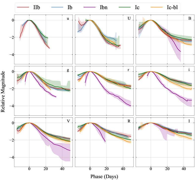
Figure 15: GP templates are shown in optical bands of $U,~{}u^{\prime},~{}B,~{}V,~{}g^{\prime},~{}R,~{}r^{\prime},~{}I,~{}i^{\prime}$ bands for each SESN subtype (as per legend at the top). Templates of different subtypes in each band are behaving mostly similarly within the uncertainties. The behavior of the templates in different bands is consistent with our expectation of the decline becoming shallower as we move to redder bands. Sudden changes in the number of light curves used to generate the templates at some epochs may lead to unphysical behaviors such as the rapid increase in the uncertainty of the Ib $U$ band template near $\sim 30$ days or the uncertainty drop in the Ic $g$ template between $\sim 35$ and $\sim 50$ days from $\mathrm{JD}_{\mathrm{Vmax}}$.

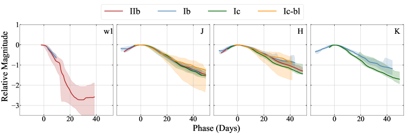
Figure 16: GP templates for the $~{}w1,J,~{}H,~{}K_{s}$ bands. There are less than three light curves in $w2,~{}m2~{}$ bands and we are not able to release a template for these bands.

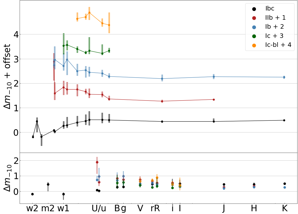
Figure 17: $\Delta m_{15}$ (left) and $\Delta m_{-10}$ (right) for our SN Ibc templates and each SESN subtype template. The location of the point on the $x$ axis is set to the effective wavelength of the filter (assuming the Swift UVOT system for ${w2,~{}m2,~{}w1}$, Johnson and SDSS filters for the $U\!BV\!RI$  and $u^{\prime}g^{\prime}r^{\prime}i^{\prime}$  respectively, and 2MASS/PAIRITEL for ${J,~{}H,~{}K_{s}}$). In the top panel, the values are separated on the vertical axis by an arbitrary value (as per legend) for readability. On the bottom panel, the values are plotted in their natural space to make the overlap and separation of measurements more obvious to the eye. We see an overall slower evolution past peak as wavelengths get longer, both in the Ibc templates and in each individual subtype template. At the bluest wavelengths ($w2$, $m2$, $w1$) the photometric measurements are too sparse and too scarse to assess any wavelength-based dependence on the evolutionary time scales. In most photometric bands, the $\Delta m_{15}$ and $\Delta m_{-10}$ are consistent for all subtypes within the uncertainties (IQR) except for the rapid post-peak evolution of SN Ib-n, discussed further in subsection 5.8 (for which measurements of $\Delta m_{15}$ only are available in selected bands). Occasionally, we see inconsistencies between the values measured for the SN Ibc templates and for the individual subtype GP templates. For example, the SN Ibc templates show a more rapid evolution at NIR wavelengths than each subtype’s template. We attribute this inconsistency to the poor quality and sparsity of photometric measurements in NIR bands. Values plotted are reported in LABEL:tab:del_m15 and LABEL:tab:del_m10. This figure is further discussed in subsection 5.4.

In the remainder of this section, we aim to investigate the behavior of the GP templates. We first compare the behavior of different subtypes relative to each other (subsection 5.4). Then, we compare the GP templates to a set of well-known simulated SN Ibc light curves from the LSST photometric simulations PLAsTiCC and ELAsTiCC (subsection 5.5). Finally, we compare the GP templates to individual SESNe to identify subclasses and peculiar SNe (subsection 5.6 and subsection 5.8).

5.3 GP Templates for SESNe Subtypes

With the individual GP fits in hand, we create templates for each subtype in the bands that have at least three light curves as the rolling median of the light curve fits (and IQR describing the uncertainty). The median is calculated within an adaptive time window. We require a larger time window at late epochs, where fewer light curves are available: the window size is three days up to $\mathrm{JD}_{\mathrm{max}}$+ 15 days, four days in the $15\leq\mathrm{JD}_{\mathrm{max}}\leq 20$ days range, five days in the $20\leq\mathrm{JD}_{\mathrm{max}}\leq 27$ days range, six days in the $27\leq\mathrm{JD}_{\mathrm{max}}\leq 35$ days range, seven days $35\leq\mathrm{JD}_{\mathrm{max}}\leq 45$ days range, and eight days thereafter. These numbers were optimized empirically. Figure 15 and Figure 16 shows the GP templates of different subtypes in each band for epochs $-20\leq\mathrm{JD}_{\mathrm{max}}\leq 40$ days along with their IQR between.

In general, there is significantly less data available for SESNe in the UV and IR when compared to optical bands. The UV in particular provides a significant challenge as stripped-envelope supernovae tend to be less UV bright than other core-collapse supernovae (Pritchard et al., 2014). We were only able to create GP templates for a single subtype in a single filter in UV frequencies: Type IIb in Swift $w1$ (the reddest UV filter) and for a fairly limited set in the IR (3/5 subtypes in $J$, 1/5 in $K_{s}$, and 2/5 in $H$).

5.4 Comparing behavior of different subtypes

We have created separate templates for different subtypes of SESNe including IIb, Ib, Ic, Ic-bl, and Ibn.

We present ${\Delta m}_{15}$ and ${\Delta m}_{-10}$ values of the GP templates in different bands in LABEL:tab:del_m15 and LABEL:tab:del_m10 and Figure 17. We generally see a progressively slower decline for all subtypes in redder bands, except for SNe Ibn (to which we will return in subsection 5.8). Otherwise, there are no statistically significant differences in evolutionary time scales near the peak. We warn the reader that this can be due to the limited size of the sample when we split the SESNe by subtype. We note that the Ibc templates measure lower values of $\Delta m_{15}$ in the reddest bands (${J,~{}H,~{}K_{s}}$) and $\Delta m_{-10}$ in the reddest bands ($u$ and $U$) than the values measured for individual subtype templates available in those bands. Barbarino et al. (2021) measured the ${\Delta m}_{15}$ and ${\Delta m}_{-10}$ of 44 spectroscopically normal SNe Ic in $R$ band and found the majority of them to have $0.2\leq{\Delta m}_{15}\leq 0.7$ and $0.1\leq{\Delta m}_{-10}\leq 0.7$. This result is consistent with the ${\Delta m}_{-10}=0.33_{-0.13}^{+0.55}$ we measure on our Ic templates. However, we measure ${\Delta m}_{15}=0.73_{-0.16}^{+0.10}$, statistically inconsistent with the slower evolving values measured by Barbarino et al. (2021),.

We investigate to what extent the SESN subtypes are photometrically distinguishable by comparing pairs of templates. We only compare templates for subtypes and bands where there are at least three light curves. Most notably, we see that Ic-bl have a faster evolution than other types at late times. Figure 18 shows a comparison of Ic and Ic-bl templates. Type Ic-bl SN are distinguishable from Ic type by the broad lines in their spectra, but they have not been known to show significantly different photometric behavior. Our templates show that these two subtypes are mostly similar within their IQR range, although in $R$, $I$, and $i$ bands, Ic-bl subtype seems to have a faster evolution starting at $\sim 20$ days, and in $B$ in phases later than 40 days. In Figure 19 and Figure 20 we see that Ic-bl are faster evolving at late times in the $R$ and $I$ band when compared to SNe Ib and IIb as well, with an even more significant separation. This may be true in other bands redder than $V$, but photometry is generally poor for SNe Ic-bl in $i$ and NIR bands, leading to large uncertainties in the template. Additional pair-wise template figures are shown in Appendix A.

Several examples of SN IIb light curves with shock-cooling double-peaked signatures have been observed in the literature (Richmond et al. 1994; Arcavi et al. 2011; Kumar et al. 2013; Morales-Garoffolo et al. 2014; Kilpatrick et al. 2016; Armstrong et al. 2021, and see review by Modjaz et al. 2019). However, we do not see a clear signature of the cooling envelope emission in our templates (Figure 20 and Appendix B). While in the $U$ SN IIb templates we do see the evidence of two peaks in the median GP time series (solid red line), the uncertainties are large in the pre-peak phases, especially in the bluer wavelengths ($U$, $B$, $g$). The large uncertainties are due to the concurrent effects of paucity and low S/N of early time data, and intrinsic diversity of SNe IIb in these phases: the cooling envelope signature is not always present, and when it is it has different time scales, consistent with different progenitor sizes. We will return to double-peaked lightcurves in subsection 5.8.

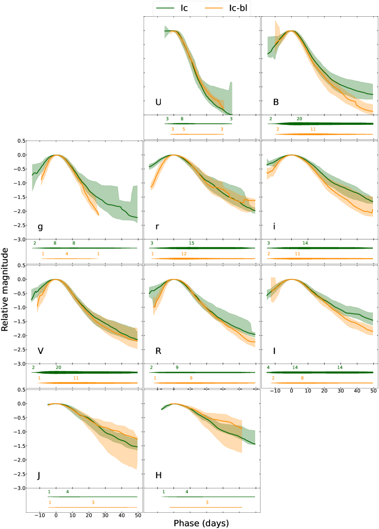
Figure 18: GP templates of subtypes Ic and Ic-bl in all the existing bands. The lower panel in each subplot shows the number of light curves that were used in each time window to create the template. We caution the reader that sharp features in the templates or their uncertainties can be connected to the sudden change in the number of the light curves used to generate the template in that band (e.g. Ic template near  40 days after $\mathrm{JD}_{\mathrm{Vmax}}$).

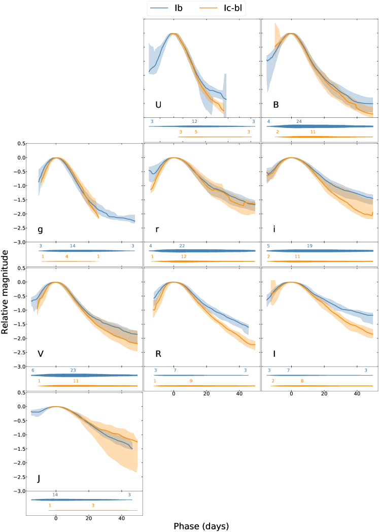
Figure 19: As Figure 18 for SN Ib and SN Ic-bl subtypes.

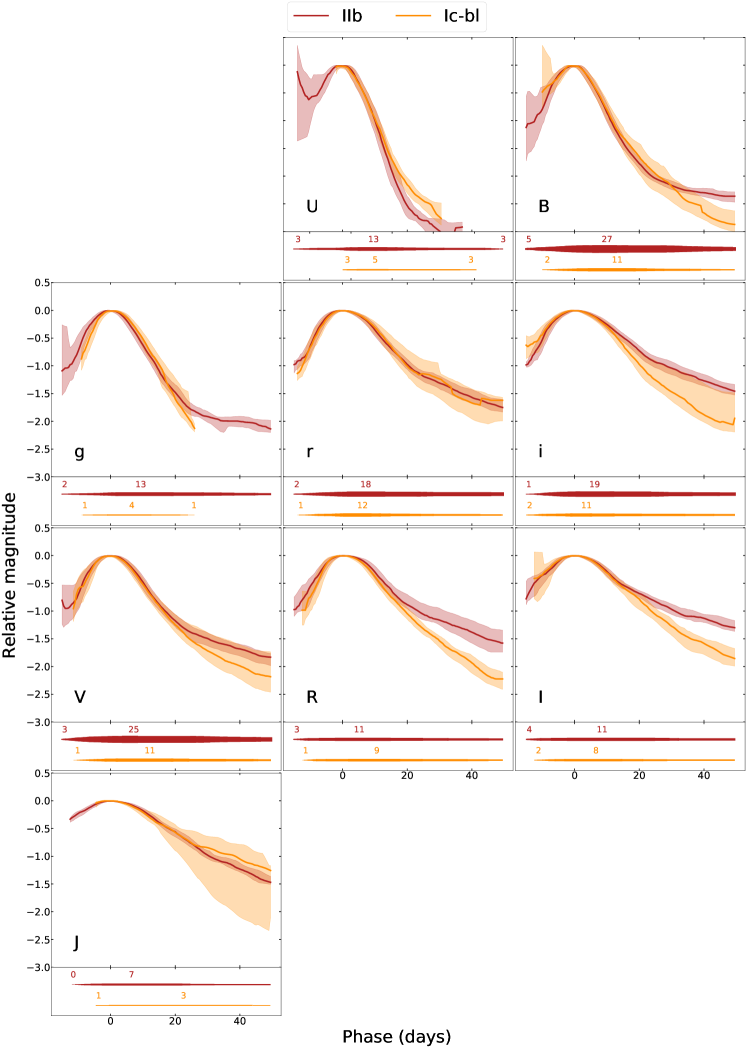
Figure 20: As Figure 18 for SN IIb and SN Ic-bl subtypes.

5.5 Comparison with SESN light curves in the PLAsTiCC and ELAsTiCC dataset

As discussed in section 1 and section 2, a motivation for our work is the development of templates that can be used to improve photometric classification of SESNe. To that end, we compare our templates to simulated LSST light curves in order to assess the accuracy of the synthetic LSST samples that are used to train photometric classifiers. The Photometric LSST Astronomical Time-Series Classification Challenge (PLAsTiCC) (Allam Jr et al., 2018) was a community-focused data challenge that took place in 2018. The challenge provided simulated light curves of millions of transients and variable stars as will be observed by the Rubin LSST. The dataset has a category of SN Ibc light curves for SESNe. Light curves for the challenge are generated following the process described in Kessler et al. 2019. Starting with an underlying SED, the SuperNova Analysis (SNANA, Kessler et al. 2009) is used to forward-model the observing process, simulating extinction, survey systematics, and observing strategy to arrive at the final synthetic multi-band photometry.

The PLAsTiCC SESNe light curves are generated using SED time series of 13 well-sampled Ibc (7 Ib and 6 Ic) combined with a parametrization obtained with the MOSFiT package (Guillochon et al., 2018).

We have selected 58 light curves from their Ibc sample that have $z<0.2$ and have at least 2 data points between phases -10 and 10 days in $r$ band. For each band use the light curve only if it has at least four data points in the $-50\leq\mathrm{JD}_{\mathrm{max}}\leq 100$ days range. We plotted this set of well-sampled simulated light curves in $u,g,r,i$ bands along with our GP templates to investigate their time evolution in Figure 21.

To align the PLAsTiCC data with the templates in brightness, we interpolate each PLAsTiCC light curve with a cubic spline. In the $u$ band, it is hard to draw a general conclusion due to the large uncertainties. Compared to our templates, the PLAsTiCC simulations show significant differences: they have light curves with slower late-time evolution, particularly in the redder bands, as well as a few extremely fast-evolving light curves.

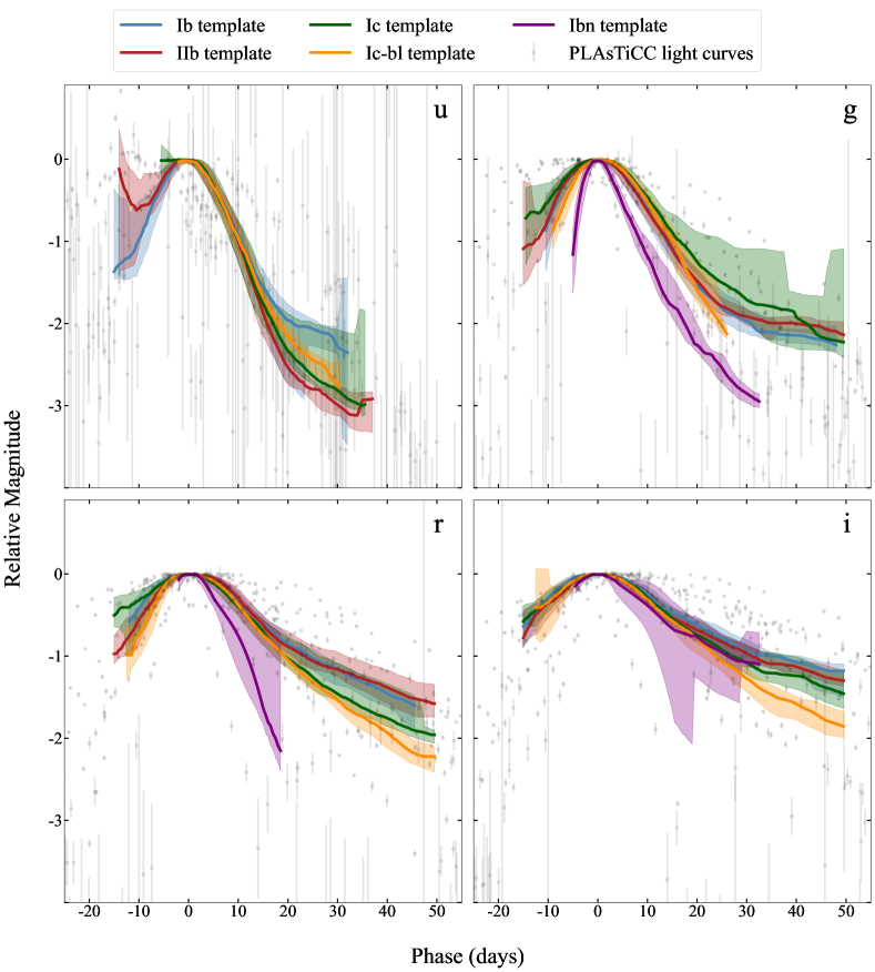
Figure 21: Our GP templates (solid lines) are plotted along with the most well-sampled PLAsTiCC  light curves of SN Ibc in $u,g,r,i$ bands (grey dots). Compared to our templates, the PLAsTiCC simulations show significant differences: they have light curves with slower late-time evolution, particularly in the redder bands, as well as a few extremely fast-evolving light curves.

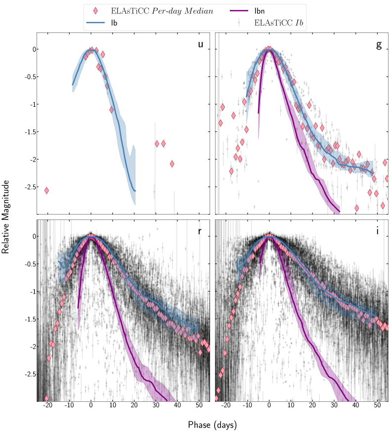
Figure 22: The GP templates of subtypes Ib (blue curve) and Ibn (purple curve) are plotted along with ELAsTiCC light curves of SN Ib in $u,g,r,i$ bands (black dots) and their per-day medians (pink diamonds). The ELAsTiCC sample is broadly consistent with the SN Ib behavior observed in our sample, although they display a larger variance. Some of the light curves in the ELAsTiCC sample have a rapid evolution broadly consistent with SNe Ibn.

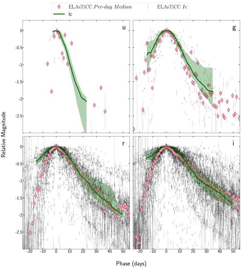
Figure 23: The GP template of subtype Ic (green curve) is plotted along with ELAsTiCC light curves of SN Ic in $u,g,r,i$ bands (black dots) and their per-day medians (pink diamonds). The ELAsTiCC sample shows a significantly more rapid rise for SN Ic than observed in our sample in the $r$ and $i$ bands. The fall is broadly consistent with the past-peak behavior of our sample, but like for Figure 22, the ELAsTiCC sample shows a larger variance than observed in our data.

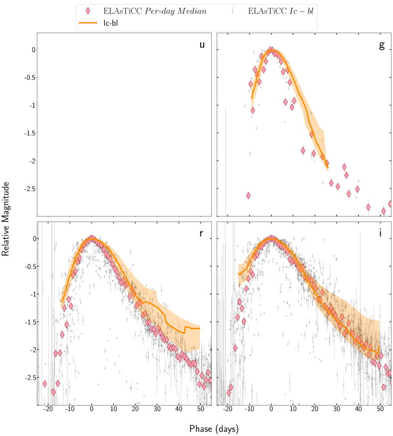
Figure 24: The GP template of subtype Ic-bl (orange curve) is plotted along with ELAsTiCC light curves of SN Ic-bl in $u,g,r,i$ bands (black dots) and their per-day medians (pink diamonds). The ELAsTiCC data shows a behavior broadly consistent with our SNe Ic-bl sample. We note a deviation in late-time behavior in $r$ band (phase $>20$ days), but our templates are rather noisy in this region.

In 2022, the next generation of LSST-related light curve simulations was released under the name of The Extended LSST Astronomical Time-Series Classification Challenge (ELAsTiCC, Narayan & ELAsTiCC Team 2023). The new simulations constitute an upgrade to the PLAsTiCC data in many ways (Lokken et al., 2023), including information about the galaxy host of transients and “alert”-level information to simulate real-time response to LSST discovery. The SESN sample here is not generated via MOSFiT, and it includes recent CC spectrophotometric templates from Vincenzi et al. 2019 (discussed in section 1).

In this dataset, the SNe Ibc are split into their subtypes: SNe Ib, SNe Ic, and SNe Ic-bl. We plot these light curves in Figure 22, Figure 23, and Figure 24 respectively. We select objects with $z<0.2$ with at least one data point between phases $-5\leq\mathrm{JD}_{\mathrm{max}}\leq 5$ days and at least five data points with $\mathrm{\emph{{S/N}}}>10$ overall. With more light curves available in this dataset, we also measure the per-day median of all the ELAsTiCC light curves in each band for each subtype. We notice general consistency between our data and the ELAsTiCC’s light curve sample, with their daily medians contained within our templates’ variance, except for SNe Ic, where our templates show a slower rise in $r$ and $i$ (ELAsTiCC’s samples in $u$ and $g$ bands are sparse and noisy at early and late times). The difference in the SN Ic early-time rise between our templates and the ELAsTiCC light curves would be problematic in real-time classifications as it raises similarity to other SN types and misleads the classifiers. We notice however the variance in the evolution of the ELAsTiCC light curves for both SN Ib and SN Ic types is far larger than the variance in our sample. The ELAsTiCC light curves for a number of SNe Ib and SNe Ic are more rapidly evolving than our observed SN Ib and SN Ic templates, and more consistent with SNe Ibn. Finally, the SN Ic-bl ELAsTiCC sample is too sparse for a detailed comparison, but it seems to generally reflect the same characteristics as the SN Ib and SN Ic samples.

There is a significant pressure in enabling photometric transient classification to advance time-domain astrophysics in the LSST era, where the spectroscopic samples will be dwarfed by the photometric samples given the lack of large-aperture dedicated spectrographs. If indeed the LSST simulated data on SESNe are inconsistent with the distribution of observed properties of these objects, this inconsistency can bias photometric classifiers trained on these datasets and lead to unrealistic expectations of accuracy. For example: the SCONE classifier (Qu & Sako, 2022), trained on the PLAsTiCC data, has a 0.11 (0.07, 0.04) contamination rate of SNe Ibc in the SN Ia samples at trigger (5 days after trigger, and 50 days after trigger respectively) and a 0.17 (0.16, 0.08) contamination of SNe Ibc in the SLSNe samples when spectroscopic information is not available. We note that SLSNe are characteristically slowly evolving and this contamination rate can be explained if the SN Ibc training sample is biased toward slow evolvers. This might lead to an underestimate of the contamination rate in SN Ia (cosmological) samples. Similarly, Gagliano et al. (2023) has developed a multi-modal SN classifier that uses galaxy information jointly with photometry for early classification of transients, is trained on ELAsTiCC and ZTF SN photometry, and we speculate that its poor performance for the SN Ibc classification may be due to the discrepancy between the ELAsTiCC simulations of SN Ibc and their real behavior.

Figure 25: GP templates for the SN IIb subtype are shown in bands $B$, $V$, $I$ (black curves) along with their IQR (grey shaded area). In each band, light curves of SNe with unusual spectroscopic or photometric features are plotted to compare their photometry with the GP templates. This figure is discussed in subsection 5.6

Figure 26: As Figure 25 for SNe Ib

Figure 27: As Figure 25 for SNe Ic

5.6 Compare GP templates with unusual supernovae

In this section, we compare our subtype templates to individual supernovae that have been claimed in the literature to show unusual features, because of their photometric or spectroscopic characteristics. We briefly discuss each SESN and the reason it is considered atypical. For SESNe identified as spectroscopically peculiar or known as peculiar in any photometric band. In Figure 25 through Figure 29, we plot their light curves in all bands where photometric measurements are available. Missing light curves in some bands are simply due to a lack of observations in that band.

Figure 25 shows our GP templates for SNe IIb in bands $B$, $V$, $R$, and $I$ (black solid line) along with their IQR (grey area). Individual unusual SNe IIb are plotted in colors and are discussed below.

• SN2013df shows flat-bottom H$\alpha$ absorption lines that could be an indication of an asymmetrical interaction between the ejecta and the CSM (Morales-Garoffolo et al., 2014). The photometry of this SN is overall consistent with our templates but their declining curves are close to the lower limit of the templates showing their rather fast decline.

• SN2010as is among a group of SNe IIb that have weak He and H lines in their early time spectra and low expansion velocities (Folatelli et al., 2014). However, its photometry is consistent with our templates.

• SN2011fu is a spectroscopically normal SN IIb that has been found to have a slow decline in late phases (Morales-Garoffolo et al., 2015b). We confirm these findings in Figure 25.

• SN2011hs is believed to be a faint SN IIb with a fast photometric rise and decline seen in Bufano et al. (2014). Compared to our templates, it is indeed showing a fast rise in $B$, $V$, and $R$ and a fast decline in $V$, $R$, and $I$ bands.

Figure 26 shows GP templates for the SN Ib subtype in bands $B$, $V$, and $R$ (black solid line) along with their IQR (grey area). Individual unusual SNe Ib are plotted in colors and are discussed below.

• SN2015ap is classified as SN Ib/c-bl and is known to have a fast evolution (Gangopadhyay et al., 2020) which we can confirm when comparing its light curve to our templates in $B$ and $V$ bands.

• SN2007uy and SN2009er are known to be peculiar SN Ib types since they show broad unusual spectroscopic features compared to the spectra of normal SNe Ib (Modjaz et al., 2014). However, the light curves of these SNe in the $B$ and $V$ filters are consistent with our GP template within the IQR.

• Calcium-rich (Ca-rich) supernovae are a subclass of SNe with spectra dominated by [Ca II] lines. There is debate over whether these SNe belong to the thermonuclear SN family (SNe Ia) or to the SESNe family (SNe Ibc) (De et al., 2021; Polin et al., 2021; Das et al., 2023) as they are often found in the outskirts of the galaxies where SNe Ia are usually found (Karthik Yadavalli et al., 2023). Additionally, De et al. (2020) finds Ca-rich SNe with spectroscopic features similar to both SNe Ibc and SNe Ia. Many of these SNe show strong He absorption lines and therefore we compare them with SNe Ib here. We have plotted photometry for three Ca-rich Ib’s in Figure 26: SN2007ke, PTF11kmb, and SN2010et. SN2007ke in the $R$ band and SN2010et in the $B$ band seem to decline faster than our templates. However, PTF11kmb in the $B$ band is within the uncertainties of our template (we discussed SN2012hn, identified as a Ca-rich Ic, later in this section).

Figure 28: As Figure 25 for SN Ic-bl.

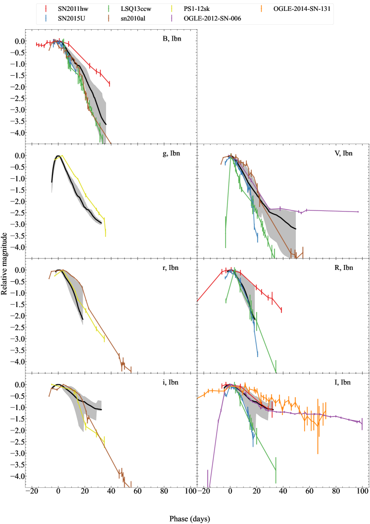
Figure 29: As Figure 25 for SN Ibn.

Figure 27 shows our GP templates for SNe Ic in bands $U\!BV\!RI$  (black solid line) along with their IQR (grey area). Individual unusual SNe Ic are plotted in colors and are discussed below.

• SN2013ge showed a double-peaked light curve pronounced in the Swift UV bands, but also somewhat in the $u$ and $B$ bands and early spectra with narrow absorption lines with high velocities (Drout et al., 2016). However, the optical photometry of this SN in redder bands ($V$$R$$I$) is generally within the uncertainties of our GP templates except for possible signatures of a slow decline in $R$.

• LSQ14efd shows a variety of unusual spectroscopic features with similarity to SNe Ic, SNe Ic-bl, and late-time SNe Ia spectra (Barbarino et al., 2017). Its photometry is however overall consistent with our GP templates.

• SN2017ein has narrow spectral lines with high velocities similar to SN2013ge (Xiang et al., 2019). The photometry of this SN is mostly consistent but at the rapid evolution end of our GP templates with clear signs of a rapid rise in $B$ and $V$, which do not show any signs of the claimed shock breakout emission that the authors claim.

• SN2012hn is believed to be a faint SN Ic with absorption features of [Ca II] in its spectra and therefore, it is classified as Ca-rich Ic (Valenti et al., 2014). The photometry of this SN shows a slightly rapid decline compared to our GP templates.

• PTF12gzk has high expansion velocities but narrow absorption lines that make it a peculiar SN Ic (Ben-Ami et al., 2012; Horesh et al., 2013). Its photometry is consistent with our templates except for the $B$ band where, however, the light curve is extremely noisy.

• SN2003id exhibits unusual spectroscopic features (Morrell & Hamuy, 2003), and its light curves show a fast decline and double-peaked rise compared to our GP templates in all bands.

• iPTF15dtg has normal SN Ic spectra (Taddia et al., 2016). Photometry is only available in the $B$ band where we find a wide photometric peak and signs of a double-peaked light curve.

• SN1994I is a well-observed SN Ic that is often claimed as a prototypical SN Ic, but compared to our templates, it has very rapid evolution which is on average two to five times the uncertainty region below the GP templates in $B$, $V$, $R$, and $I$ bands. Both the fast rise and fast decline of SN 1994I have been mentioned before in D11 and B14.

Figure 28 shows our GP templates for the SN Ic-bl subtype in bands $B$, $V$, $R$, and $I$ (black solid line) along with their IQR (grey area). Individual unusual type Ic-bl SESNe are plotted in colors and are discussed below.

• a GRB afterglow contaminates item SN2013cq in early phases (Melandri et al., 2014) and it has a flat smooth decline compared to our templates due to the GRB afterglow, which is a power law.

• SN2010bh is a spectroscopically normal SN Ic-bl with GRB but it appears to have higher velocities at late phases compared to other SNe of this type (Chornock et al., 2010; Modjaz et al., 2016). It also appears consistent with, although at the rapid evolution end of, our template in $B$ and $V$ band where photometry is available.

• SN2009bb is known to be a peculiar SN Ic-bl due to the claimed presence of He in its early spectra (though it is not very convincing) and its associated radio emission (Pignata et al., 2011). The photometry of this SN shows a slightly faster decline than our template in all bands.

• SN2006aj is a SN Ic-bl associated with GRB 060218 (Mirabal et al., 2006). Light curves of this SN (available in $B$ and $V$ only) show the signature of shock breakout and have a faster decline compared to our templates.

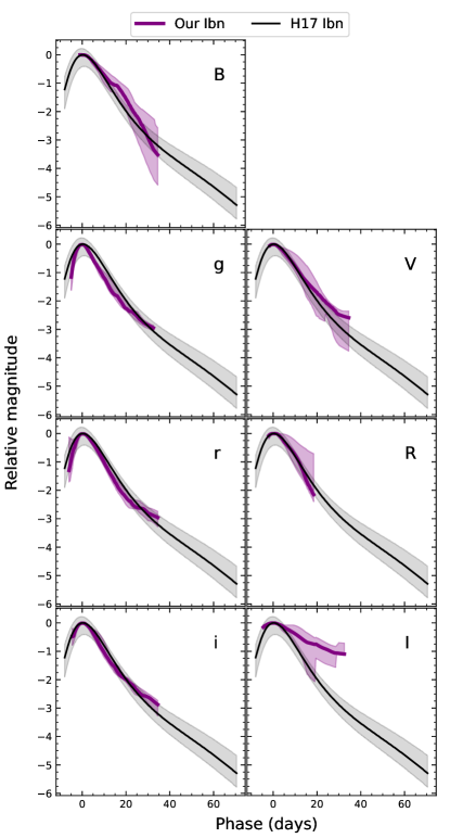
Figure 30: GP templates for SNe Ibn in $B$, $g$, $V$, $r$, $R$, $i$, and $I$ bands (purple curves) are plotted along with the H17 SN Ibn template, which is the same in all bands. The behavior of H17’s SN Ibn template is mostly consistent with our SN Ibn template within the uncertainty. A faster rise in $g$ and $r$, where we have early data, is observed. However, the $g$ data that generates this template is selected for its rapid evolution (subsection 5.8), introducing a selection bias that may explain the discrepancy.

5.7 SESNe Ibn

A small subset of type Ib SESNe show narrow helium emission lines, thus SN Ibn, which are due to interaction between SN ejecta and helium-rich circumstellar material (CSM) (Hosseinzadeh et al. 2017, hereafter H17, Hosseinzadeh et al. 2019). We created and presented here the first photometric templates for these types of supernovae in 7 bands (a broadband template was presented in H17). Our sample of SNe Ibn includes 8 SESNe from the OSNC and 6 SESNe from a sample of ZTF objects that were released in Ho23. Note that the ZTF sample includes photometry in $g$ and $r$ bands, and $i$ band at a lower cadence, thus our SN Ibn templates in these bands will be mostly dominated by the ZTF sample.

The ZTF sample includes SESNe that appear brighter than half of their maximum brightness for less than 12 days (Ho23). The inclusion of these data in our sample, even those that appeared in the literature after OSNC stopped being updated, allows us to increase our SN Ibn sample size and produce templates for this subtype. However, note that not all objects in this sample are SNe Ibn. Only spectroscopically confirmed SN Ibn are used to create our SN Ibn GP templates (the other light curves in Ho23 are compared with our templates in subsection 5.8).

Figure 29 shows GP templates for SNe Ibn in bands $B$, $g$, $V$, $R$, $r$, $I$, and $i$ (black solid line) and their IQR (grey area). Along with the templates, we plot all of the SN Ibn light curves in our sample except for the ZTF objects (Ho23) since these SNe were explicitly selected for their fast-evolving light curves. We note the relatively slow evolution of SNe Ibn 2011hw, OGLE-2012-SN-006, and OGLE-2014-SN-131, compared to these templates in $g$, $r$, and $i$ bands. We also see the particularly rapid evolution of LSQ13ccw, faster than our template in all bands available ($B$, $V$, $R$, and $I$), and of SN2015U, which is faster at all times in $I$ and at late times in $V$ compared to our templates. Note that the SN Ibn template in the $g$ band is smoother and with smaller uncertainty regions since the slow-evolving SNe Ibn in our sample did not have $g$ band data and is dominated by the ZTF sample. This introduces a selection bias, as light curves in this sample are explicitly selected for their rapid evolution.

H17 also presents a SN Ibn template which is generated by combining all existing photometry, including photometry in different bands, of 18 SNe Ibn. This average template is created, as ours, fitting the combined light curves with a GP in logarithmic time. The sample includes light curves mostly in $r$/$R$ band, and a few objects in $V$ (1), $g$ (1), $I$ (1), and $z$ (1) bands. Their uncertainty regions are created by fitting the positive and negative residuals and selecting the %95 probability region. For comparison, we plot their template along with our SN Ibn templates in all of the 7 bands in Figure 30. The templates are consistent within the uncertainty, except in the $g$ band, where we observe a faster rise in our template, and in the $I$ band we see a much slower decline in our template compared to the H17 SN Ibn template, but our uncertainties are very large, and our time baseline very short. The selection bias discussed in the previous paragraph explains this discrepancy.

5.8 Comparison with fast-evolving ZTF objects

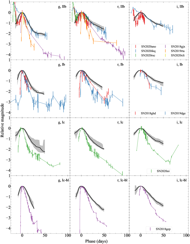
Figure 31: Comparison of the fast-evolving SESNe from Ho23 with our GP templates of the same subtype as the spectroscopic SN classification (from top to bottom, SN IIb, SN Ib, SN Ic, SN Ic-bl. This figure is discussed in subsection 5.6

In Figure 31, we show light curves of the fast-evolving SESN from Ho23 that are not classified as SNe Ibn, and thus not used to construct our templates and compare them with our templates. In summary, all SNe Ib, Ic, and Ic-bl from Ho23’s rapidly evolving sample rise and fall more rapidly than any of our GP subtype templates, as expected based on their selection criteria, even though they were spectroscopically classified squarely within the four main subtypes. We focus our analysis on the frequently observed presence of two peaks in this sample. We address two questions. We discuss whether the peaks of light curves in Ho23 are in fact due to shock cooling emission as suggested by Ho23 and answer the question of whether the ⁵⁶Ni-powered light curve did in fact have a fast evolution compared to our template.

The decay of ⁵⁶Ni to ⁵⁶Co is commonly believed to be responsible for powering the light curves of most thermonuclear and stripped-envelope SNe, including SESNe (Arnett, 1982). The peak magnitude of the light curve would then be dependent on the total ⁵⁶Ni mass, while the ejecta velocity and mass jointly control the rise and decay rates in this simple model (for applications to SESN see Taddia et al., 2018; Prentice et al., 2019). However, we occasionally observe two peaks in the SESN light curves, particularly those of SNe IIb. Pre-maximum lightcurve peaks are due primarily to two related phenomena: shock breakout, or the associated cooling of an extended envelope heated by the shock (e.g. Chevalier & Fransson, 2008; Waxman & Katz, 2017; Sapir & Waxman, 2017; Piro et al., 2021). Shock breakout refers to when the shockwave generated by the collapsing star core breaks through the star’s surface. This produces an intense, short-lived ($\sim$minutes) flash of radiation at high-frequency wavelengths (X-rays through UV). Shock breakout signatures have been observed for SNe Ic-bl associated with GRB SN2006aj (Campana et al., 2006; Li, 2007), SN Ib SN2008D (Soderberg et al., 2008; Modjaz et al., 2009), and SN IIb SN2016gkg (Bersten et al., 2018).

The direct detection of a shock breakout is only possible when the progenitor is compact and observations at short wavelengths are available on time scales of minutes to $\leq 1$ hour after the explosion. The outer layers of the star, heated by the passage of the shock wave, continue to expand and cool down over time emitting radiation in the UV and optical wavelengths that manifests as an early (pre-$\mathrm{JD}_{\mathrm{max}}$) peak with slower ($\sim$days) evolutionary time scales. This emission is called cooling-envelope or shock cooling and in some cases, it can involve the interaction of the shock with a dense circumstellar wind rather than a stellar envelope (e.g., SN 2020bio Pellegrino et al., 2023). In what follows, we will refer to it as shock cooling emission to differentiate it from the ⁵⁶Ni-driven peak, without further speculation on the specific mechanisms that generated it. For a detailed discussion of observational shock breakout and cooling-envelope/shock-cooling emission in SESNe see the review by Modjaz et al. 2019 and reference therein. Several of the lightcurves in Ho23 showed two peaks. This prompted us to extend the baseline of the light curves presented in Ho23 to ensure we could probe and investigate the frequency and characteristics of these double-peaked signatures in this sample.

We note that the Ho23 aligned the light curves on the first peak they observed. To ensure that the full light curve evolution is captured (including any potential 2nd peaks), we downloaded the ZTF forced photometry of 9 SNe from Ho23 including 6 SNe IIb: SN2018gjx, SN2019rta, SN2020ikq, SN2020xlt, SN2020ano, and SN2020rsc, two SNe Ib: SN2019dge, SN2018ghd, and one SN Ic: SN2020oi. In most cases, the resulting light curves show some differences from Ho23. published in Ho23. In the case of SN 2019rta, and SN 2020rsc, for example, the ZTF forced photometry provided us with a longer time baseline and, in several cases, it results in lightcurves with less scatter compared to the Ho23’s published photometry (e.g., SN 2018ghd, where we also obtained the lightcurve in $i$ band, SN 2018gjx, etc). We plot these light curves along with our GP templates in Figure 31. Each row shows one subtype in bands $g$, $r$, and $i$.

SNe IIb: We observed double-peaked light curves for half of the Ho23 sample classified spectroscopically as SNe IIb, where two peaks, phenomenologically consistent with a shock cooling followed by ⁵⁶Ni evolution are clearly observed for three out of the six SNe IIb. The first row of Figure 31 shows SNe IIb from Ho23 along with our GP SN IIb templates.

SN2020ano and SN2020ikq have prominent early peaks that could be associated with a shock cooling emission (as discussed in Ho23). Our retrieved ZTF forced photometry shows a second peak also for SN2020rsc in $r$, which was not fully visible in Ho23’s photometry. We have fitted a second-order polynomial to the second peak to estimate its peak time and magnitude.

We compare the three SNe IIb with double peaks (SN2020ikq, SN2020ano, SN2020rsc) with our templates aligning them by the $\mathrm{JD}_{\mathrm{max}}$ derived from the second peak to test if the ⁵⁶Ni-driven part of the light curves shows a rapid evolution. For SN2020ikq the (presumably) ⁵⁶Ni evolution is consistent with our SN IIb template in all bands. This object does not seem to have rapidly-evolving ⁵⁶Ni -powered light curve. It does however have an extended shock cooling first peak which in the $i$ band fully hides the second peak. Note that this means that if we only had $i$ band data we would have assumed this is a single peak fast-evolving SN IIb. We will return to this point in section 6. For SN2020rsc, we see both peaks in the $r$ band where the evolution of the (presumably) ⁵⁶Ni-driven peak is consistent with typical SNe IIb  (we note that in $g$ we only have data for the shock-cooling portion of the light curve and that the $r$ band photometry we retrieved looks somewhat different from Ho23’s, in addition to have a longer baseline that straddles the second peak.) SN2020ano is marginally consistent with a typical SN IIb in the $r$ band but the photometric uncertainties are large and the evolution is more rapid than our SN IIb templates in both $g$ and $i$.

SNe IIb SN2018gjx, SN2019rta are confirmed as fast-evolving SNe with no detected second peak out to at least $\sim 80$ days after maximum.

The light curve of SN2020xlt is too limited to ascertain the presence of a single or double peak.

In summary, SN2020ano is the only double-peaked SN in this sample where the (presumably) ⁵⁶Ni evolution is atypically rapid. Two of the six rapid evolving SNe IIb in Ho23 appear to be typical SNe IIb with shock-cooling signatures: SN2020rsc and SN2020ikq are consistent with normal SNe IIb with cooling envelope emission followed by ⁵⁶Ni evolution. The shock-cooling phase is evolving more rapidly than the ⁵⁶Ni ones and drives the selection of these objects in the Ho23 sample.

SNe Ib: For SNe Ib SN2019dge and SN2018ghd, we find only one peak for each SN. Although the photometry shows a rise at phase $\sim 75$ days for SN2019dge in $g$ and $r$ bands, and for SN2018ghd in $r$ band, we do not think that those data points indicate ⁵⁶Ni peak and they are too far from the first peak and the uncertainties are very large. While we cannot determine conclusively whether this single peak is powered by shock cooling emission, by the decay of ⁵⁶Ni  or by interaction, we nevertheless align the light curves of these SNe Ib with our SN Ib template to explore their behavior. We find that the peaks of these two SNe have a faster rise and decay than our SN Ib templates in all filters.

SNe Ic and SNe Ic-bl: SN Ic 2020oi is shown in the third row and SN Ic-bl 2018gep in the last row of Figure 31. Both show only one peak in their light curves. We find that these two SNe are more rapidly evolving than the respective templates. Please note that SN2020oi in the original photometry from Ho23 had a couple of data points showing the possible start of a rise in $i$ band around phase $75$ days. In forced photometry, these points disappeared.

If, with a sufficient baseline and sufficiently dense photometry no second peak is observed, then these findings would be highly interesting: if the single peak is due to shock-cooling emission then the absence of the ⁵⁶Ni-powered peak indicates the production of a small amount of ⁵⁶Ni in these rapidly evolving CC SNe (even smaller than seen in SN2020bio, Pellegrino et al. 2023). For example, Ho23 suggested cooling emission from a shock that broke out of a massive shell of dense CSM as the powering source for SN Ic-bl 2018gep, as confirmed by Pritchard et al. (2021). Note the high absolute luminosity of SN 2018gep ($M_{V}\sim-19.53\pm 0.23$ mag), which places it between the typical brightness of SLSNe and SNe Ic-bl. If the single, rapidly-evolving peak is in fact due to decay of ⁵⁶Ni, then the Ho23 sample may uncover a new population of SESNe that have very low ejecta masses; Rho et al. (2021) modeled SN Ic 2020oi ($M_{V}\sim-15$, Gagliano et al. 2022) to have very low ejecta and very low ⁵⁶Ni masses. Samples of SESNe selected for their rapid photometric evolution result in collections that, in spite of similar light curve width, include objects with different evolutionary drivers. Note that these objects have very similar photometric evolution to SN 1994I, which, as discussed in subsection 5.6, has long been considered a prototypical SN Ic  while in fact its photometry is all but typical. SN 1994I would be included in fast-evolving SESN samples selected by photometric cuts. To better understand the nature of this subclass of SESNe, a bonafide sample of SNe Ibc should be a focus of future studies.

6 Summary and Conclusion

In the era of large surveys, like the ongoing ZTF and upcoming LSST, photometric classification is critical, as spectrographs will only be able to follow up a small fraction of the tens of thousands of transients that LSST will detect every night (Ivezić et al., 2019; Malz et al., 2019). With the goal of enhancing our knowledge of photometric behavior of less common SNe to address this need, we have produced two kinds of photometric templates for SESNe spanning UV through NIR bands, for subtypes IIb, Ib, Ic, Ic-bl, and Ibn using a dataset of open-access light curves of 165 SESNe, all SESNe in the OSNC that have at least five data points in one band, sampling over the peak, and reliable classification, augmented by a small dataset of SN Ibn light curves from the ZTF.

We have generated generic SESN templates, i.e. SN Ibc templates, by aggregating all subtypes in each of the ${w2,~{}m2,~{}w1,~{}U,~{}u,~{}B,~{}g,~{}V,~{}r,~{}R,~{}i,~{}I,~{}J,~{}H,~{}K_{s}}$ bands and computing a weighted rolling median (Figure 7). We identify a photometric bias towards bright objects that have lower measurement errors in templates generated based on weighted means, as commonly done in the literature (e.g., Drout et al. 2011). This bias produces templates with overestimated magnitudes at late times where the bias is not suppressed by large sample sizes (see the comparison in Figure 6). We advocate that templates should be generated from a more reliable statistical aggregate as we have done in this work, namely median and inter-quartile range (IQR, section 4).

For the subtype-specific templates generated with GP, we separated the SESNe family into IIb, Ib, Ic, Ic-bl, and Ibn and generated templates per band combining Gaussian Processes (GP) fits of the light curves (section 5). GPs provide a flexible statistical framework for modeling light curves, allowing us to place them on a fine grid in time, accounting for uncertainties and gaps in data, and leveraging a physics-informed model for the correlation between the data points. We have developed a robust approach to combine the light curves in our dataset that are observed with different instruments and under different conditions and to fill in gaps in the observations. Our method results in well-fitted GP models for light curves of each SESN in our sample leading to templates that allow us to study time-dependent characteristics of these classes and identify outliers. Our final set of GP templates consists of 54 templates for all subtypes: SNe IIb (in 12 bands), SNe Ib (in 13 bands), SNe Ic (in 12 bands), SNe Ic-bl (in 10 bands), and SNe Ibn (in 7 bands). Using GP fits of individual SESN in our sample allows us to take into account the diversity of all the existing photometric observations. Doing the GP fits in logarithmic time results in better fits to the early time-evolution of the SESNe. A customized objective function in the GP fit that penalizes rapid variations provides smooth fits that avoid unphysically rapid magnitude changes. In addition, aggregating the GP fits using a rolling median statistics and defining uncertainty regions using the IQR allow us to prevent biases towards brighter SESNe with lower uncertainties.

Comparing subtype templates (subsection 5.4) reveals that within the currently available data, the photometric evolution of different SESNe subtypes are mostly consistent with each other within their uncertainties, with the most notable differences being evidence of shock cooling emission in the early-time behavior of SNe IIb  (e.g., Figure 32, $U$ band) and the notably fast decline of SNe Ic-bl compared to SNe of types Ib, IIb, and Ic as shown in Figure 18, Figure 19, and Figure 20.

We compare GP templates of each subtype of SESN with the SN Ibn GP templates that we generated using data from OSNC and Ho23 (see subsection 5.7). We find that, formally, in the $r$ and $i$ bands, the decline rate as measured by $\Delta m_{15}$ is higher for SNe Ibn, and inconsistent with the decline rate of the rest of the SESN family at the 2$\sigma$ confidence level: $\Delta m_{15}(r,\mathrm{Ibc})=0.60^{+0.19}_{-0.17}$ $vs$ $\Delta m_{15}(r,\mathrm{Ibn})=1.70^{+0.14}_{-0.15}$ and $\Delta m_{15}(i,\mathrm{Ibc})=0.36^{+0.11}_{-0.10}$ $vs$ $\Delta m_{15}(i,\mathrm{Ibn})=1.56^{+0.19}_{-0.11}$ (see LABEL:tab:del_m15 and LABEL:tab:del_m10).

Our templates are valuable in evaluating the consistency and veracity of the ensemble behavior of simulated light curve samples of SESNe. This is particularly important when developing classifiers for SESN subtypes in the era of large surveys like LSST when spectroscopic observations for most objects will not be available. Thus, we compared our GP templates with SN Ibc light curves from the PLAsTiCC and ELAsTiCC simulated data sets (subsection 5.5), which provide a sandbox dataset to train photometric classification models, and found that in the PLAsTiCC sample, a significant number of objects had slower rise and decline than observed in our SESNe sample. In the more recent ELAsTiCC simulations, this issue is largely improved and the per-day median of the simulated light curves is generally consistent with our templates. However, the ELAsTiCC light curves of SNe Ic have a slower rise than our GP SN Ic templates, and those of SNe Ic-bl have a faster decline at later epochs compared to our GP SN Ic-bl templates.

Next, we compared both types of our templates (SN Ibc and GP-based subtype-specific templates) to individual SESN with known unusual photometric and/or spectroscopic characteristics to assess if they appear as outliers compared to our templates (subsection 4.1 and subsection 5.6). We find that abnormal spectroscopic behavior does not necessarily result in unusual photometric evolution (for e.g., SN2007uy, SN2009er, SN2010as, SN2013ge, LSQ14efd). Our templates also confirm that a well-known and well-observed SESN like SN1994I, which is claimed to be the prototypical SN Ic, is in fact photometrically well outside of the uncertainty region of the GP templates for SNe Ic (2-to-8 times the uncertainty region) and SN Ibc templates (2-to-7 times IQR) altogether in $B$, $V$, $R$, and $I$ (Figure 10 and Figure 27).

When analyzing the sample of rapidly evolving SESN presented in Ho23 and comparing it with our templates we identified at least two normally evolving SNe IIb in the sample, both with shock-cooling emission (SN2020rsc, SN2020ikq) that were not recognized as such in Ho23. This results from aligning our SN IIb templates by a second peak in Ho23’s sample, when present, which in some cases required extending the photometric baseline presented in Ho23 to reveal a second peak consistent with ⁵⁶Ni evolutionary time scales for normal SNe IIb. We emphasize the importance of distinguishing the evolution of early peaks, (e.g., due to shock cooling or interaction) from the ⁵⁶Ni driven peaks to disentangle the physical processes that may lead to rapid evolution. When photometry is sparse, limited to some bands, or seasonality only allows for a short light curve to be collected, the presence of two peaks may be difficult to ascertain. Since the duration of the lightcurve can probe physical processes including ⁵⁶Ni production and ejecta mass, misidentifying shock cooling signatures for ⁵⁶Ni evolution may skew statistics on SN evolution and progenitor characterization and impair inference on the true nature of the evolutionary drivers.

While being curated and updated, the OSNC was aggregating SN data, including photometry, from all publications into a single publicly accessible repository. While at the time of writing the OSNC still contains most published SESNe data, many more SESNe have been observed in the past few years. Some light curves are available only in papers dedicated to one or a few objects, and the very significant effort required to compile a truly complete sample of SESNe is beyond the scope of this paper. Without claiming completeness, we believe we have leveraged the vast majority of published SESN photometry. Other projects like WISeREP (Yaron & Gal-Yam, 2012) are engaging in similar efforts of collecting and making available published data for SNe. This is a difficult and time-consuming work, which requires infrastructural support that is difficult to obtain and sustain (as demonstrated by the loss of the OSNC). We hope our work can highlight the importance of funding and maintaining similar efforts to make open data accessible that are indispensable to enable these kinds of studies.

While at this time, our conclusions remain limited by the availability of data (the templates could not be generated for all SESN subtypes in all bands, and even where they are generated they may be noisy due to the paucity of data), our models and templates are designed to be easily updated to incorporate a growing sample SESNe. We have made our code and instructions on how to update templates publicly available and accessible.

Since light curves of different subtypes of SESNe are used to probe outstanding questions about their progenitors (Lyman et al., 2016; Taddia et al., 2018; Prentice et al., 2019; Karamehmetoglu et al., 2023), our work, which includes a larger sample of SESNe than any of these, sets the stage for probing the diversity of their explosion properties, stripping channels and progenitor rates.

7 Acknowledgment

We used the following software packages: pandas (McKinney et al., 2011), numpy (Harris et al., 2020), matplotlib (Hunter, 2007), and george (Foreman-Mackey, 2015).

The authors wish to thank Saurabh Jha for insightful discussions and suggestions and Kevin Krisciunas for providing the unpublished NIR photometry of SN 1999ex. The authors acknowledge the support of the Vera C. Rubin Legacy Survey of Space and Time Science Collaborations and particularly of the Transient and Variable Star Science Collaboration (TVS SC) that provided opportunities for collaboration and exchange of ideas and knowledge. This publication was made possible through the support of an LSSTC Catalyst Fellowship to S.K., funded through Grant 62192 from the John Templeton Foundation to LSST Corporation. The opinions expressed in this publication are those of the authors and do not necessarily reflect the views of LSSTC or the John Templeton Foundation. M.M. acknowledges support in part from ADAP program grant No. 80NSSC22K0486, from the NSF grant AST-2206657 and from the HST GO program HST-GO-16656. C.L. acknowledges support from the National Science Foundation Graduate Research Fellowship under grant No. DGE-2233066.

This research has made use of the Open SuperNova Catalog (OSNC), NASA’s Astrophysics Data System Bibliographic Services (ADS), the HyperLEDA database and the NASA/IPAC Extragalactic Database (NED) which is operated by the Jet Propulsion Laboratory, California Institute of Technology, under contract with the National Aeronautics and Space Administration.

Appendix A Additional Figures

Figure 32, Figure 33, and Figure 34 are similar to Figure 18, Figure 19 and Figure 20 and show a comparison of the pairs of (SN Ib, SN IIb), (SN Ib, SN Ic), and (SN IIb, SN Ic) templates in all the bands where both subtypes have a template. These figures indicate that the photometric evolution of these subtype pairs are mostly consistent with each other within the uncertainty regions.

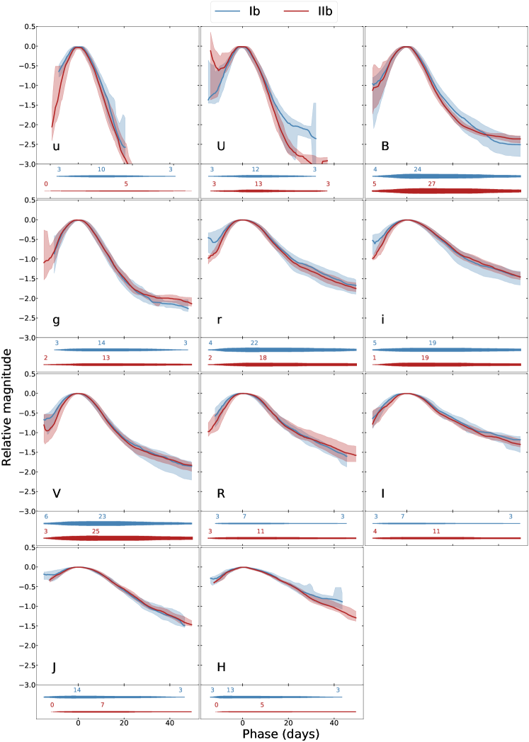
Figure 32: As Figure 18 for Ib and IIb subtypes.

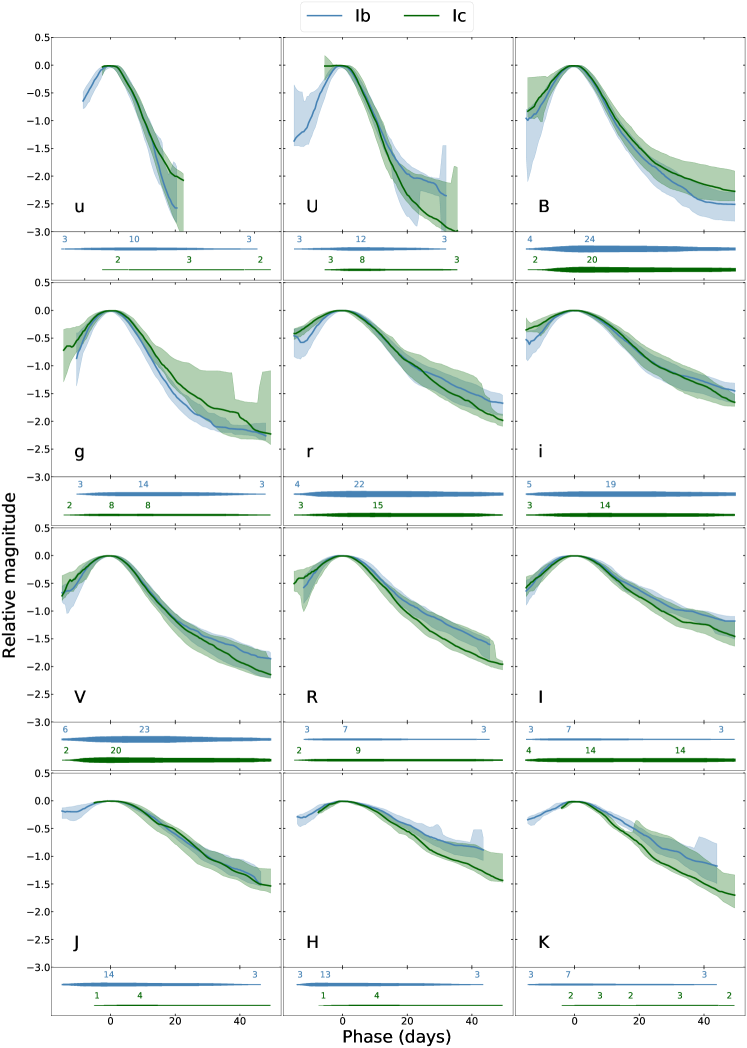
Figure 33: As Figure 18 for Ib and Ic subtypes.

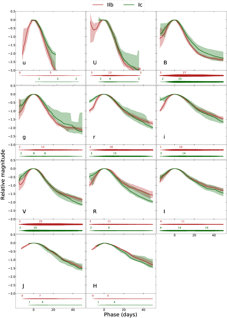
Figure 34: As Figure 18 for IIb and Ic subtypes.

Figure 35 shows the evolution of relative colors for each subtype template in phases -10, 0, 10, 20, 30 days since $\mathrm{JD}_{\mathrm{max}}$. The trend in color seems similar for all subtypes and is only different for SN Ibn subtype in $V$-$r$ and $V$-$i$ colors, but those have large uncertainties and therefore we cannot draw a definite conclusion from them.

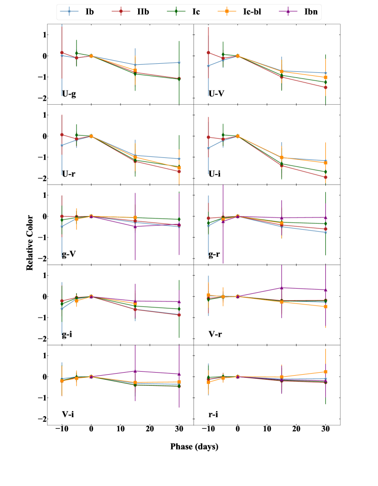
Figure 35:

Appendix B Additional Tables

LABEL:tab:OPT1, LABEL:tab:OPT2, and LABEL:tab:UVNIR include information about the photometry in our SESNe sample. For each SN, the type, number of photometric data points per band, minimum and maximum epochs of the photometry per band, and the median S/N per band are shown.

Table 4: Templates SESNe sample UBVRI photometric epochs details

	Type	U	B	V	R	I
Name		N, [min,max], SNR	N, [min,max], SNR	N, [min,max], SNR	N, [min,max], SNR	N, [min,max], SNR
SN1954A	Ib	5, [52.5,109.8], 575.7	58, [-7.8,343.5], 575.7	44, [44.5,109.8], 575.7	-	-
SN1962L	Ib-c	11, [-9.8,18.0], 575.7	93, [-15.8,78.0], 575.7	11, [-9.8,18.0], 575.7	-	-
SN1983N	Ib	6, [11.2,18.2], 575.7	27, [-10.2,18.2], 575.7	56, [-10.8,170.8], 575.7	-	-
SN1983V	Ic	-	8, [-15.8,237.5], 575.7	5, [-15.8,29.2], 575.7	-	-
SN1984I	Ib	11, [-4.0,31.8], 575.7	18, [-17.0,20.8], 575.7	14, [-4.0,20.8], 575.7	-	-
SN1985F	Ib-c	-	18, [-16.8,321.2], 575.7	20, [253.8,444.5], 575.7	-	-
SN1991N	Ic	-	3, [2.5,15.5], 575.7	9, [-4.0,18.5], 575.7	-	-
SN1993J	IIb	191, [-17.8,737.2], 575.7	401, [-18.8,737.2], 575.7	459, [-18.8,737.2], 575.7	398, [-18.5,737.2], 575.7	365, [-18.5,642.5], 575.7
SN1994I	Ic	11, [-5.0,9.8], 575.7	52, [-7.0,59.8], 287.8	111, [-7.0,62.8], 575.7	98, [-7.0,62.8], 575.7	90, [-7.0,62.8], 575.7
SN1996cb	IIb	-	34, [-14.2,70.5], 575.7	45, [-14.2,139.2], 575.7	46, [-14.2,139.2], 575.7	-
SN1997ef	Ic-bl	-	6, [-11.8,23.0], 575.7	43, [-12.2,143.0], 191.9	8, [-15.2,110.2], 575.7	-
SN1998bw	Ic-bl	22, [-7.5,401.2], 575.7	131, [-14.2,486.5], 575.7	167, [-15.5,521.5], 575.7	65, [-15.5,521.5], 575.7	140, [-7.8,521.5], 575.7
SN1999dn	Ib	11, [-2.8,104.8], 95.9	14, [-2.8,121.8], 115.1	16, [-2.8,370.0], 143.9	16, [-2.8,370.0], 115.1	13, [-2.8,121.8], 95.9
SN1999ex	Ib	86, [-19.8,8.2], 457.1	134, [-19.8,20.2], 509.2	138, [-19.8,20.2], 479.7	136, [-19.8,20.2], 549.5	134, [-19.8,20.2], 479.7
SN2001ig	IIb	-	1, [-18.0,-18.0], 575.7	4, [-18.0,124.8], 575.7	7, [-7.2,243.0], 575.7	-
SN2002ap	Ic-bl	105, [-9.8,29.0], 575.7	227, [-9.8,306.2], 575.7	739, [-9.8,325.2], 575.7	331, [-9.8,306.2], 575.7	242, [-9.8,306.2], 575.7
SN2002ji	Ib	-	-	-	11, [-8.0,71.8], 575.7	-
SN2003bg	IIb	-	19, [-20.5,298.8], 239.9	23, [-18.5,298.8], 250.3	11, [-19.8,298.8], 287.8	17, [-10.5,298.8], 250.3
SN2003dh	Ic-bl	55, [-12.0,-6.0], 287.8	333, [-12.5,26.8], 119.9	384, [-12.5,26.8], 191.9	1644, [-12.8,67.0], 122.5	350, [-12.5,19.0], 112.9
SN2003id	Ic-pec	-	12, [-8.8,28.0], 91.7	20, [-8.8,34.0], 153.9	21, [-8.8,34.0], 255.8	20, [-8.8,34.0], 164.7
SN2003jd	Ic-bl	-	12, [-0.5,71.2], 120.0	16, [-1.5,74.2], 185.9	15, [1.5,74.2], 147.6	18, [-1.5,74.2], 165.0
SN2003lw	Ic-bl	-	-	4, [-4.8,68.0], 335.8	10, [-9.8,68.0], 385.5	11, [-9.8,66.2], 383.8
SN2004aw	Ic	16, [-5.8,85.2], 51.4	56, [-5.8,255.2], 78.0	64, [-5.8,255.2], 115.1	66, [-5.8,345.2], 143.9	56, [-5.8,255.2], 129.5
SN2004dn	Ic	-	15, [-10.2,52.8], 35.8	15, [-10.0,82.0], 48.9	15, [-10.0,82.0], 143.5	15, [-10.0,82.0], 112.4
SN2004dk	Ib	-	16, [-24.2,293.8], 265.0	16, [-24.2,293.8], 22.3	16, [-24.2,293.8], 246.4	15, [-24.2,293.8], 415.3
SN2004ex	IIb	-	22, [-15.0,48.0], 338.6	24, [-15.0,55.0], 397.5	-	-
SN2004ff	IIb	-	17, [-4.2,68.8], 190.0	15, [-4.2,57.5], 338.6	-	-
SN2004fe	Ic	-	25, [-9.5,43.2], 205.6	26, [-9.5,43.2], 287.8	-	-
SN2004gq	Ib	10, [-10.2,83.5], 38.7	40, [-10.2,75.8], 274.1	44, [-10.2,83.5], 479.7	-	-
SN2004gt	Ic	-	24, [-6.2,134.8], 169.3	28, [-6.2,134.8], 287.8	-	-
SN2004gv	Ib	-	18, [-10.5,32.2], 413.3	21, [-10.5,32.2], 411.2	-	-
SN2005az	Ic	-	5, [-8.0,76.0], 72.9	11, [-8.0,88.0], 143.9	-	-
SN2005bf	Ib	100, [-27.2,27.8], 116.3	116, [-31.2,70.5], 274.1	129, [-31.2,70.5], 303.0	-	-
SN2005by	IIb	-	10, [-2.2,28.8], 15.2	19, [-2.2,69.8], 17.1	18, [-2.2,66.8], 28.0	18, [-2.2,77.8], 30.3
SN2005em	IIb	-	9, [-3.8,36.2], 159.9	11, [-3.8,59.2], 191.9	-	-
SN2005hg	Ib	30, [-12.8,25.2], 60.0	31, [-12.8,82.2], 99.2	44, [-12.8,127.0], 151.6	-	-
SN2005kl	Ic	-	14, [-3.8,154.2], 17.7	33, [-3.8,138.0], 43.3	-	-
SN2005kz	Ic	-	6, [-2.5,16.5], 20.0	8, [-2.5,17.5], 95.2	-	-
SN2005mf	Ic	4, [0.5,5.5], 26.9	19, [-0.5,65.2], 25.4	23, [-0.5,65.2], 63.3	-	-
SN2006T	IIb	4, [-4.2,21.8], 21.9	58, [-14.2,108.5], 274.1	62, [-14.2,108.5], 411.2	-	-
SN2006aj	Ic-bl	62, [-10.0,22.2], 79.9	77, [-10.0,23.0], 76.8	71, [-10.0,24.2], 54.3	-	-
SN2006ba	IIb	-	12, [-2.2,36.8], 65.0	22, [-2.2,65.8], 90.0	-	-
SN2006bf	IIb	-	6, [-2.8,22.2], 67.6	17, [-2.8,48.2], 106.6	-	-
SN2006cb	Ib	-	1, [3.2,3.2], 60.6	5, [2.2,19.2], 52.8	-	-
SN2006el	IIb	-	15, [0.2,46.0], 47.6	32, [0.2,110.8], 82.9	-	-
SN2006ep	Ib	-	24, [-8.8,68.0], 120.4	39, [-8.8,106.2], 115.6	-	-
SN2006fo	Ib	-	20, [-1.8,87.2], 130.9	34, [-1.8,133.0], 99.3	-	-
SN2006ir	Ib-c	-	6, [2.5,70.2], 212.8	22, [1.5,85.2], 177.2	-	-
SN2006lc	Ib	1, [-7.0,-7.0], 18.6	13, [-7.8,38.2], 79.9	22, [-7.8,45.2], 138.7	-	-
SN2007C	Ib	2, [-3.0,-1.2], 56.8	37, [-3.0,126.5], 125.1	51, [-3.0,136.8], 179.9	-	-
SN2007I	Ic-bl	-	8, [-0.5,40.2], 41.8	21, [-0.5,70.2], 81.1	-	-
SN2007d	Ic-bl	-	6, [-5.5,15.2], 29.0	9, [-5.5,21.2], 29.8	-	-
SN2007Y	Ib	18, [-12.5,20.8], 70.7	37, [-12.5,32.5], 111.8	37, [-12.5,39.5], 87.2	-	-
SN2007ag	Ib	-	9, [-0.5,29.2], 67.7	14, [-0.5,40.5], 163.0	-	-
SN2007ay	IIb	-	3, [-5.8,-1.8], 230.3	5, [-6.8,15.2], 274.1	-	-
SN2007ce	Ic-bl	-	9, [0.0,18.0], 137.1	17, [0.0,54.0], 191.9	-	-
SN2007cl	Ic	-	6, [-6.0,27.2], 60.3	23, [-6.0,63.0], 179.9	-	-
SN2007gr	Ic	54, [-8.8,153.0], 205.6	128, [-8.8,182.2], 239.9	129, [-8.8,401.2], 261.7	80, [-8.8,401.2], 230.3	76, [-8.8,401.2], 230.3
SN2007ke	Ib-Ca	-	4, [2.2,35.2], 21.6	4, [2.2,37.5], 35.3	7, [-11.5,13.5], 48.0	-
SN2007kj	Ib	-	28, [-6.0,51.2], 66.1	32, [-6.0,51.2], 110.9	-	-
SN2007ru	Ic-bl	9, [-3.5,29.5], 143.9	44, [-3.5,59.5], 143.9	36, [-3.5,210.8], 221.4	22, [-3.5,210.8], 256.0	19, [-3.5,150.0], 274.7
SN2007rz	Ic	-	15, [-10.8,40.2], 40.0	21, [-10.8,64.2], 112.9	-	-
SN2007uy	Ib-pec	17, [-10.0,13.2], 61.2	79, [-10.8,134.0], 81.1	83, [-10.8,134.0], 101.0	-	-
SN2008d	Ib	39, [-18.0,12.5], 30.8	110, [-19.8,121.0], 92.9	115, [-19.8,100.0], 122.5	18, [-19.8,12.2], 575.7	18, [-19.8,12.2], 575.7
SN2008aq	IIb	9, [-7.2,7.8], 74.8	36, [-7.2,120.8], 209.8	38, [-7.2,120.8], 281.0	-	-
SN2008ax	IIb	28, [-19.5,33.0], 68.7	76, [-19.5,305.0], 143.9	98, [-18.5,305.0], 191.9	41, [-17.5,305.0], 191.9	33, [-17.5,305.0], 191.9
SN2008bo	IIb	9, [-8.5,11.0], 38.1	61, [-9.8,107.0], 57.0	68, [-9.8,107.0], 82.8	-	-
SN2008cw	IIb	-	7, [2.2,28.0], 37.1	7, [2.2,28.0], 60.0	-	-
SN2009K	II	-	13, [-20.8,258.5], 442.8	13, [-20.8,258.5], 523.3	-	-
SN2009bb	Ic-bl	2, [-9.2,4.5], 16.8	64, [-9.2,48.8], 115.1	87, [-9.2,113.8], 86.1	47, [-9.2,71.8], 191.9	47, [-9.2,71.8], 95.9
SN2009er	Ib-pec	-	13, [-0.8,23.2], 88.6	16, [-1.5,23.2], 185.9	-	-
SN2009iz	Ib	4, [-12.0,-7.8], 52.8	35, [-13.2,72.5], 92.8	35, [-13.2,135.5], 221.4	-	-
SN2009jf	Ib	13, [-18.0,27.8], 143.9	63, [-18.0,247.0], 213.2	62, [-18.0,247.0], 319.8	33, [-18.0,247.0], 261.7	33, [-18.0,247.0], 205.6
SN2009mg	IIb	18, [-13.0,52.2], 42.4	22, [-13.0,52.2], 63.3	22, [-13.0,52.2], 68.5	-	-
SN2009mk	IIb	9, [-10.5,5.5], 20.2	13, [-10.5,13.8], 38.9	18, [-10.5,34.0], 41.9	-	-
SN2010ay	Ic-bl	-	-	-	6, [-18.0,26.8], 86.3	-
SN2010bh	Ic-bl	-	14, [-9.2,24.0], 105.5	11, [-5.0,25.5], 191.9	-	-
SN2010al	Ibn	10, [0.5,20.5], 72.0	26, [-7.0,46.0], 83.8	28, [-7.0,55.0], 63.0	-	-
SN2010as	IIb	-	31, [-13.2,70.5], 133.9	25, [-13.2,100.5], 274.1	25, [-13.2,100.5], 338.6	24, [-13.2,100.5], 319.8
SN2010cn	Ic	6, [-7.8,3.2], 31.8	7, [-7.8,4.8], 37.1	7, [-7.8,4.8], 24.7	-	-
SN2010et	Ib-Ca	-	5, [-0.8,8.2], 25.0	-	-	-
PTF10qts	Ic-bl	-	4, [-4.5,22.5], 57.1	-	24, [-14.5,55.5], 167.9	-
SN2010jr	IIb	22, [-15.5,53.0], 45.5	31, [-15.5,51.5], 48.0	30, [-15.5,51.5], 40.1	-	-
SN2011am	Ib	10, [-6.5,11.0], 37.6	15, [-6.5,31.2], 55.3	15, [-6.5,31.2], 58.2	-	-
SN2011bm	Ic	27, [-15.8,81.2], 48.0	43, [-16.8,269.5], 64.0	45, [-16.8,269.5], 64.0	45, [-16.8,269.5], 72.0	45, [-16.8,269.5], 82.2
SN2011dh	IIb	90, [-17.2,152.2], 116.3	158, [-17.2,222.5], 143.9	821, [-19.0,289.2], 221.4	78, [-17.0,289.2], 287.8	81, [-17.0,220.2], 191.9
PTF11iqb	IIn	-	10, [1.5,117.2], 130.9	10, [1.5,117.2], 123.9	255, [-12.8,552.0], 575.7	51, [-9.8,138.2], 91.4
SN2011ei	IIb	14, [-10.5,9.0], 51.7	21, [-10.5,28.0], 36.9	21, [-10.5,28.0], 32.9	-	-
PTF11kmb	Ib-Ca	-	4, [3.0,9.0], 60.8	-	-	-
PTF11qcj	Ic-bl	-	-	-	54, [24.8,110.5], 575.7	-
SN2011fu	IIb	21, [-14.2,65.8], 95.9	45, [-14.2,105.5], 191.9	54, [-14.2,141.5], 287.8	58, [-14.2,150.5], 287.8	60, [-14.2,150.5], 191.9
SN2011hg	IIb	5, [-9.0,3.2], 33.7	8, [-9.0,8.8], 44.0	8, [-9.2,8.8], 32.9	-	-
SN2011hs	IIb	17, [-8.5,27.2], 66.2	41, [-8.8,210.8], 115.1	44, [-8.8,210.8], 287.8	21, [-11.2,210.8], 575.7	14, [-8.8,210.8], 575.7
SN2011hw	Ibn	5, [-16.5,-8.5], 81.1	13, [-16.5,38.8], 52.3	5, [-16.5,-8.5], 49.2	80, [-154.0,350.0], 575.7	6, [-6.2,31.8], 52.3
SN2012P	IIb	6, [-11.2,4.0], 42.8	32, [-7.0,152.8], 63.6	4, [-0.8,4.0], 69.1	-	-
SN2012ap	Ic-bl	7, [-6.8,7.5], 28.4	26, [-8.8,22.2], 51.7	26, [-8.8,22.2], 77.1	17, [-8.8,20.2], 143.9	15, [-2.8,22.2], 143.9
PS1-12sk	Ibn	1, [9.8,9.8], 57.6	1, [9.8,9.8], 57.6	1, [9.8,9.8], 44.3	-	-
SN2012au	Ib	12, [-5.0,31.8], 105.5	12, [-5.0,31.8], 115.1	12, [-5.0,31.8], 143.9	-	-
SN2012hn	Ic-Ca	4, [-1.5,7.5], 28.8	18, [-1.5,34.5], 92.9	30, [-1.5,184.8], 110.9	40, [-1.5,234.8], 82.2	34, [-1.5,234.8], 133.2
SN2012cd	IIb	-	-	-	26, [-12.8,13.2], 575.7	-
SN2012bz	IIb	-	-	-	2, [-6.2,-1.2], 76.8	1, [-15.2,-15.2], 72.0
PTF12gzk	Ic-pec	1, [-2.8,-2.8], 61.9	13, [-11.2,4.0], 99.2	13, [-9.0,3.5], 159.9	35, [-17.2,4.0], 383.8	16, [-9.0,4.0], 191.9
PTF12hni	Ic	-	7, [6.0,75.0], 24.0	-	-	-
OGLE-2012-sn-006	Ibn	9, [96.8,185.5], 64.0	11, [15.8,180.5], 64.0	46, [-1.2,186.5], 105.5	34, [15.8,180.5], 95.9	192, [-104.0,370.8], 143.9
SN2013ak	IIb	15, [-5.8,30.0], 68.5	15, [-5.8,30.0], 92.8	15, [-5.8,30.0], 97.6	-	-
SN2013cu	II	9, [-7.0,12.8], 76.8	8, [-2.0,21.5], 70.7	8, [-2.0,21.5], 43.0	3, [-8.5,-8.2], 575.7	-
SN2013cq	Ic-bl	-	24, [-17.0,28.0], 72.0	24, [-17.0,28.0], 143.9	24, [-17.0,28.0], 143.9	24, [-17.0,28.0], 143.9
SN2013df	IIb	66, [-13.5,41.0], 70.7	84, [-16.5,230.2], 82.2	86, [-16.5,606.0], 95.9	46, [-18.8,606.0], 115.1	37, [-14.5,606.0], 95.9
iPTF13bvn	Ib	27, [-14.8,42.8], 57.6	96, [-15.0,199.8], 92.8	94, [-15.0,199.8], 143.9	70, [-14.8,262.8], 191.9	71, [-14.8,262.8], 143.9
SN2013dk	Ic	6, [-8.5,4.8], 27.3	7, [-8.5,8.8], 51.9	7, [-8.5,8.8], 61.2	-	-
LSQ13ccw	Ibn	-	22, [3.2,33.5], 31.1	30, [-3.5,33.5], 35.2	10, [-3.2,34.5], 30.3	9, [3.2,34.5], 24.0
OGLE-2013-sn-091	Ic	-	-	-	-	26, [-222.5,137.8], 21.4
SN2013ge	Ic	45, [-14.0,36.2], 91.4	104, [-13.2,159.2], 143.9	113, [-13.2,159.2], 115.1	12, [-12.5,19.5], 95.9	12, [-12.5,19.5], 83.9
OGLE-2013-sn-134	Ic	-	-	-	-	31, [-283.2,112.5], 46.0
SN2014C	Ib	12, [-7.5,5.8], 37.4	12, [-4.2,5.8], 76.8	11, [-4.2,5.8], 87.2	-	-
SN2014L	Ic	26, [-10.2,56.5], 115.1	53, [-10.5,80.5], 82.2	67, [-10.5,141.2], 191.9	74, [-10.5,141.2], 143.9	74, [-10.5,141.2], 191.9
OGLE-2014-sn-014	Ib	-	-	-	-	34, [-111.5,251.5], 44.8
SN2014ad	Ic-bl	30, [-10.8,79.0], 224.4	29, [-10.8,79.0], 319.8	29, [-10.8,79.0], 442.8	28, [-10.8,79.0], 303.0	28, [-10.8,79.0], 303.0
LSQ14efd	Ic	-	10, [-10.8,23.5], 38.4	34, [-17.0,63.8], 38.4	9, [-3.8,73.8], 27.4	9, [-3.8,73.8], 30.3
OGLE-2014-sn-131	Ibn	-	-	-	-	46, [-61.5,249.8], 38.4
ASASSN-14ms	Ib	3, [-1.0,1.0], 137.1	3, [-1.0,1.0], 122.5	26, [-6.0,25.0], 81.1	-	-
SN2015U	Ibn	-	22, [-3.8,13.2], 58.5	29, [-3.8,20.8], 111.7	31, [-3.8,20.8], 140.6	27, [-3.8,18.2], 124.2
OGLE15eo	Ic	-	-	-	-	56, [-376.0,173.8], 53.3
SN2015ap	Ib/c-bl	11, [-12.0,16.0], 72.9	11, [-12.0,16.0], 82.2	11, [-12.0,16.0], 71.1	-	-
OGLE15jy	Ib-c	-	-	-	-	22, [-218.2,133.8], 25.1
OGLE15rb	Ic	-	-	-	-	26, [-361.2,97.8], 30.2
iPTF15dtg	Ic	-	10, [-15.8,7.0], 94.4	-	-	-
OGLE15vk	Ic	-	-	-	-	23, [-471.5,54.2], 60.6
SN2016gkg	IIb	28, [-19.0,39.8], 78.9	89, [-19.8,81.5], 111.8	169, [-20.5,81.5], 72.0	27, [-18.5,81.5], 143.9	27, [-19.5,81.5], 143.9
OGLE16ekf	IIb	-	-	-	-	31, [-269.2,187.5], 24.8
SN2017ein	Ic	-	51, [-15.2,50.8], 117.5	49, [-13.2,49.8], 262.2	52, [-15.2,51.8], 383.8	20, [22.8,50.8], 442.8
SN2019all	Ib-c	-	-	-	-	33, [-323.8,373.2], 18.6
SN2019aajs	Ibn	-	4, [7.0,28.2], 56.0	4, [7.0,28.2], 28.8	-	-
SN2019pik	Ic	-	-	-	-	21, [-57.8,149.8], 47.2

References

- Aigrain & Foreman-Mackey (2023) Aigrain, S., & Foreman-Mackey, D. 2023, Annual Review of Astronomy and Astrophysics, 61, 329
- Allam Jr et al. (2018) Allam Jr, T., Bahmanyar, A., Biswas, R., et al. 2018, arXiv preprint arXiv:1810.00001
- Ambikasaran et al. (2014) Ambikasaran, S., Foreman-Mackey, D., Greengard, L., Hogg, D. W., & O’Neil, M. 2014, ArXiv e-prints. https://arxiv.org/abs/1403.6015
- Arcavi (2017) Arcavi, I. 2017, in Handbook of Supernovae, ed. A. W. Alsabti & P. Murdin, 239, doi: 10.1007/978-3-319-21846-5_39
- Arcavi et al. (2011) Arcavi, I., Gal-Yam, A., Yaron, O., et al. 2011, The Astrophysical Journal Letters, 742, L18, doi: 10.1088/2041-8205/742/2/L18
- Armstrong et al. (2021) Armstrong, P., Tucker, B. E., Rest, A., et al. 2021, MNRAS, 507, 3125, doi: 10.1093/mnras/stab2138
- Arnett (1982) Arnett, W. D. 1982, ApJ, 253, 785, doi: 10.1086/159681
- Barbarino et al. (2017) Barbarino, C., Botticella, M. T., Dall’Ora, M., et al. 2017, Monthly Notices of the Royal Astronomical Society, 471, 2463
- Barbarino et al. (2021) Barbarino, C., Sollerman, J., Taddia, F., et al. 2021, Astronomy & Astrophysics, 651, A81
- Bellm et al. (2018) Bellm, E. C., Kulkarni, S. R., Graham, M. J., et al. 2018, Publications of the Astronomical Society of the Pacific, 131, 018002
- Ben-Ami et al. (2012) Ben-Ami, S., Gal-Yam, A., Filippenko, A. V., et al. 2012, The Astrophysical Journal Letters, 760, L33
- Benetti et al. (2011) Benetti, S., Turatto, M., Valenti, S., et al. 2011, Monthly Notices of the Royal Astronomical Society, 411, 2726
- Bernstein et al. (2012) Bernstein, J. P., Kessler, R., Kuhlmann, S., et al. 2012, ApJ, 753, 152, doi: 10.1088/0004-637X/753/2/152
- Bersten et al. (2018) Bersten, M. C., Folatelli, G., García, F., et al. 2018, Nature, 554, 497, doi: 10.1038/nature25151
- Bersten et al. (2018) Bersten, M. C., Folatelli, G., García, F., et al. 2018, Nature, 554, 497
- Bianco et al. (2014) Bianco, F. B., Modjaz, M., Hicken, M., et al. 2014, ApJS, 213, 19, doi: 10.1088/0067-0049/213/2/19
- Blondin et al. (2007) Blondin, S., Modjaz, M., Kirshner, R., Challis, P., & Calkins, M. 2007, Central Bureau Electronic Telegrams, 800
- Boone (2019) Boone, K. 2019, The Astronomical Journal, 158, 257
- Bufano et al. (2012) Bufano, F., Pian, E., Sollerman, J., et al. 2012, ApJ, 753, 67, doi: 10.1088/0004-637X/753/1/67
- Bufano et al. (2014) Bufano, F., Pignata, G., Bersten, M., et al. 2014, MNRAS, 439, 1807, doi: 10.1093/mnras/stu065
- Campana et al. (2006) Campana, S., Mangano, V., Blustin, A. J., et al. 2006, Nature, 442, 1008–1010, doi: 10.1038/nature04892
- Cano (2013a) Cano, Z. 2013a, MNRAS, 434, 1098, doi: 10.1093/mnras/stt1048
- Cano (2013b) —. 2013b, MNRAS, 434, 1098, doi: 10.1093/mnras/stt1048
- Cano (2014) —. 2014, ApJ, 794, 121, doi: 10.1088/0004-637X/794/2/121
- Chevalier & Fransson (2008) Chevalier, R. A., & Fransson, C. 2008, The Astrophysical Journal, 683, L135
- Chornock et al. (2010) Chornock, R., Berger, E., Levesque, E. M., et al. 2010, arXiv preprint arXiv:1004.2262
- Ciabattari et al. (2011) Ciabattari, F., Mazzoni, E., Jin, Z., et al. 2011, Central Bureau Electronic Telegrams, 2827, 1
- Ciabattari et al. (2013) Ciabattari, F., Mazzoni, E., Donati, S., et al. 2013, Central Bureau Electronic Telegrams, 3557, 1
- Clocchiatti & Wheeler (1997) Clocchiatti, A., & Wheeler, J. 1997, The Astrophysical Journal, 491, 375
- Das et al. (2023) Das, K. K., Kasliwal, M. M., Fremling, C., et al. 2023, ApJ, 959, 12, doi: 10.3847/1538-4357/acfeeb
- De et al. (2021) De, K., Fremling, U. C., Gal-Yam, A., et al. 2021, ApJ, 907, L18, doi: 10.3847/2041-8213/abd627
- De et al. (2020) De, K., Kasliwal, M. M., Tzanidakis, A., et al. 2020, The Astrophysical Journal, 905, 58
- Drout et al. (2016) Drout, M., Milisavljevic, D., Parrent, J., et al. 2016, The Astrophysical Journal, 821, 57
- Drout et al. (2011) Drout, M. R., Soderberg, A. M., Gal-Yam, A., et al. 2011, The Astrophysical Journal, 741, 97, doi: 10.1088/0004-637X/741/2/97
- Fan et al. (2011) Fan, Y.-Z., Zhang, B.-B., Xu, D., Liang, E.-W., & Zhang, B. 2011, ApJ, 726, 32, doi: 10.1088/0004-637X/726/1/32
- Filippenko (1997) Filippenko, A. V. 1997, Annual Review of Astronomy and Astrophysics, 35, 309, doi: 10.1146/annurev.astro.35.1.309
- Filippenko et al. (1993) Filippenko, A. V., Matheson, T., & Ho, L. C. 1993, The Astrophysical Journal, 415, L103, doi: 10.1086/187043
- Folatelli et al. (2014) Folatelli, G., Bersten, M. C., Kuncarayakti, H., et al. 2014, The Astrophysical Journal, 792, 7
- Foreman-Mackey (2015) Foreman-Mackey, D. 2015, Astrophysics Source Code Library, ascl
- Gagliano et al. (2023) Gagliano, A., Contardo, G., Mackey, D. F., Malz, A. I., & Aleo, P. D. 2023, arXiv preprint arXiv:2305.08894
- Gagliano et al. (2022) Gagliano, A., Izzo, L., Kilpatrick, C. D., et al. 2022, ApJ, 924, 55, doi: 10.3847/1538-4357/ac35ec
- Gal-Yam (2016) Gal-Yam, A. 2016, arXiv preprint arXiv:1611.09353
- Gal-Yam et al. (2002) Gal-Yam, A., Ofek, E. O., & Shemmer, O. 2002, MNRAS, 332, L73, doi: 10.1046/j.1365-8711.2002.05535.x
- Gangopadhyay et al. (2020) Gangopadhyay, A., Misra, K., Sahu, D., et al. 2020, Monthly Notices of the Royal Astronomical Society, 497, 3770
- Guillochon et al. (2018) Guillochon, J., Nicholl, M., Villar, V. A., et al. 2018, The Astrophysical Journal Supplement Series, 236, 6
- Guillochon et al. (2016) Guillochon, J., Parrent, J., & Margutti, R. 2016, ArXiv e-prints. https://arxiv.org/abs/1605.01054
- Harris et al. (2020) Harris, C. R., Millman, K. J., Van Der Walt, S. J., et al. 2020, Nature, 585, 357
- Hložek et al. (2020) Hložek, R., Ponder, K., Malz, A., et al. 2020, arXiv preprint arXiv:2012.12392
- Ho et al. (2023) Ho, A. Y., Perley, D. A., Gal-Yam, A., et al. 2023, The Astrophysical Journal, 949, 120
- Horesh et al. (2013) Horesh, A., Kulkarni, S. R., Corsi, A., et al. 2013, The Astrophysical Journal, 778, 63
- Hosseinzadeh et al. (2019) Hosseinzadeh, G., McCully, C., Zabludoff, A. I., et al. 2019, The Astrophysical Journal Letters, 871, L9
- Hosseinzadeh et al. (2017) Hosseinzadeh, G., Arcavi, I., Valenti, S., et al. 2017, The Astrophysical Journal, 836, 158
- Hunter (2007) Hunter, J. D. 2007, Computing in science & engineering, 9, 90
- Ivezić et al. (2019) Ivezić, Ž., Kahn, S. M., Tyson, J. A., et al. 2019, The Astrophysical Journal, 873, 111
- Karamehmetoglu et al. (2023) Karamehmetoglu, E., Sollerman, J., Taddia, F., et al. 2023, A&A, 678, A87, doi: 10.1051/0004-6361/202245231
- Karthik Yadavalli et al. (2023) Karthik Yadavalli, S., Villar, V. A., Izzo, L., et al. 2023, arXiv e-prints, arXiv:2308.12991, doi: 10.48550/arXiv.2308.12991
- Kessler et al. (2009) Kessler, R., Bernstein, J. P., Cinabro, D., et al. 2009, PASP, 121, 1028, doi: 10.1086/605984
- Kessler et al. (2019) Kessler, R., Narayan, G., Avelino, A., et al. 2019, Publications of the Astronomical Society of the Pacific, 131, 094501
- Kessler et al. (2019) Kessler, R., Narayan, G., Avelino, A., et al. 2019, PASP, 131, 094501, doi: 10.1088/1538-3873/ab26f1
- Kilpatrick et al. (2016) Kilpatrick, C. D., Foley, R. J., Abramson, L. E., et al. 2016, Monthly Notices of the Royal Astronomical Society, 465, 4650, doi: 10.1093/mnras/stw3082
- Krige (1951) Krige, D. G. 1951, Journal of the Chemical, Metallurgical and Mining Society of South Africa, 52, 119, doi: 10.2307/3006914
- Kulkarni (2013) Kulkarni, S. 2013, The Astronomer’s Telegram, 4807, 1
- Kumar et al. (2013) Kumar, B., Pandey, S. B., Sahu, D. K., et al. 2013, MNRAS, 431, 308, doi: 10.1093/mnras/stt162
- Kumar et al. (2013) Kumar, B., Pandey, S. B., Sahu, D. K., et al. 2013, Monthly Notices of the Royal Astronomical Society, 431, 308, doi: 10.1093/mnras/stt162
- Law et al. (2009) Law, N. M., Kulkarni, S. R., Dekany, R. G., et al. 2009, Publications of the Astronomical Society of the Pacific, 121, 1395
- Li (2007) Li, L.-X. 2007, Monthly Notices of the Royal Astronomical Society, 375, 240
- Liu & Modjaz (2014) Liu, Y., & Modjaz, M. 2014, ArXiv e-prints. https://arxiv.org/abs/1405.1437
- Liu et al. (2017) Liu, Y.-Q., Modjaz, M., & Bianco, F. B. 2017, ApJ, 845, 85, doi: 10.3847/1538-4357/aa7f74
- Liu et al. (2016) Liu, Y.-Q., Modjaz, M., Bianco, F. B., & Graur, O. 2016, The Astrophysical Journal, 827, 90
- Lokken et al. (2023) Lokken, M., Gagliano, A., Narayan, G., et al. 2023, MNRAS, 520, 2887, doi: 10.1093/mnras/stad302
- Lyman et al. (2016) Lyman, J., Bersier, D., James, P., et al. 2016, Monthly Notices of the Royal Astronomical Society, 457, 328
- Malesani et al. (2009) Malesani, D., Fynbo, J. P. U., Hjorth, J., et al. 2009, ApJ, 692, L84, doi: 10.1088/0004-637X/692/2/L84
- Malz et al. (2019) Malz, A. I., Hložek, R., Allam, T., J., et al. 2019, AJ, 158, 171, doi: 10.3847/1538-3881/ab3a2f
- McAllister et al. (2017) McAllister, M. J., Littlefair, S. P., Dhillon, V. S., et al. 2017, MNRAS, 464, 1353, doi: 10.1093/mnras/stw2417
- McKinney et al. (2011) McKinney, W., et al. 2011, Python for high performance and scientific computing, 14, 1
- Melandri et al. (2014) Melandri, A., Pian, E., D’elia, V., et al. 2014, Astronomy & Astrophysics, 567, A29
- Mirabal et al. (2006) Mirabal, N., Halpern, J., An, D., Thorstensen, J., & Terndrup, D. 2006, The Astrophysical Journal Letters, 643, L99
- Modjaz et al. (2019) Modjaz, M., Gutiérrez, C. P., & Arcavi, I. 2019, Nature Astronomy, 3, 717
- Modjaz et al. (2016) Modjaz, M., Liu, Y. Q., Bianco, F. B., & Graur, O. 2016, The Astrophysical Journal, 832, 108
- Modjaz et al. (2009) Modjaz, M., Li, W., Butler, N., et al. 2009, The Astrophysical Journal, 702, 226
- Modjaz et al. (2014) Modjaz, M., Blondin, S., Kirshner, R. P., et al. 2014, AJ, 147, 99, doi: 10.1088/0004-6256/147/5/99
- Morales-Garoffolo et al. (2014) Morales-Garoffolo, A., Elias-Rosa, N., Benetti, S., et al. 2014, Monthly Notices of the Royal Astronomical Society, 445, 1647, doi: 10.1093/mnras/stu1837
- Morales-Garoffolo et al. (2014) Morales-Garoffolo, A., Elias-Rosa, N., Benetti, S., et al. 2014, MNRAS, 445, 1647, doi: 10.1093/mnras/stu1837
- Morales-Garoffolo et al. (2015a) Morales-Garoffolo, A., Elias-Rosa, N., Bersten, M., et al. 2015a, MNRAS, 454, 95, doi: 10.1093/mnras/stv1972
- Morales-Garoffolo et al. (2015b) —. 2015b, MNRAS, 454, 95, doi: 10.1093/mnras/stv1972
- Morrell & Hamuy (2003) Morrell, N., & Hamuy, M. 2003, International Astronomical Union Circular, 8203, 2
- Najita et al. (2016) Najita, J., Willman, B., Finkbeiner, D. P., et al. 2016, arXiv preprint arXiv:1610.01661
- Narayan & ELAsTiCC Team (2023) Narayan, G., & ELAsTiCC Team. 2023, in American Astronomical Society Meeting Abstracts, Vol. 55, American Astronomical Society Meeting Abstracts, 117.01
- Nowogrodzki (2019) Nowogrodzki, A. 2019, Nature, 571, 133
- Oates et al. (2012) Oates, S. R., Bayless, A. J., Stritzinger, M. D., et al. 2012, MNRAS, 424, 1297, doi: 10.1111/j.1365-2966.2012.21311.x
- Okyudo et al. (1993) Okyudo, M., Kato, T., Ishida, T., Tokimasa, N., & Yamaoka, H. 1993, PASJ, 45, L63
- Orellana & Bersten (2022) Orellana, M., & Bersten, M. C. 2022, A&A, 667, A92, doi: 10.1051/0004-6361/202244124
- Pastorello et al. (2015) Pastorello, A., Benetti, S., Brown, P. J., et al. 2015, MNRAS, 449, 1921, doi: 10.1093/mnras/stu2745
- Pellegrino et al. (2023) Pellegrino, C., Hiramatsu, D., Arcavi, I., et al. 2023, The Astrophysical Journal, 954, 35
- Pellegrino et al. (2023) Pellegrino, C., Hiramatsu, D., Arcavi, I., et al. 2023, ApJ, 954, 35, doi: 10.3847/1538-4357/ace595
- Perley et al. (2020) Perley, D. A., Fremling, C., Sollerman, J., et al. 2020, ApJ, 904, 35, doi: 10.3847/1538-4357/abbd98
- Phillips (1993) Phillips, M. M. 1993, The Astrophysical Journal, 413, L105
- Pian et al. (2017) Pian, E., Tomasella, L., Cappellaro, E., et al. 2017, Monthly Notices of the Royal Astronomical Society, 466, 1848
- Pietra (1955) Pietra, S. 1955, Mem. Soc. Astron. Italiana, 26, 185
- Pignata et al. (2011) Pignata, G., Stritzinger, M., Soderberg, A., et al. 2011, ApJ, 728, 14, doi: 10.1088/0004-637X/728/1/14
- Piro (2015) Piro, A. L. 2015, ApJ, 808, L51, doi: 10.1088/2041-8205/808/2/L51
- Piro et al. (2021) Piro, A. L., Haynie, A., & Yao, Y. 2021, The Astrophysical Journal, 909, 209
- Polin et al. (2021) Polin, A., Nugent, P., & Kasen, D. 2021, ApJ, 906, 65, doi: 10.3847/1538-4357/abcccc
- Prentice et al. (2016) Prentice, S., Mazzali, P., Pian, E., et al. 2016, Monthly Notices of the Royal Astronomical Society, 458, 2973
- Prentice et al. (2019) Prentice, S. J., Ashall, C., James, P. A., et al. 2019, MNRAS, 485, 1559, doi: 10.1093/mnras/sty3399
- Press & Teukolsky (1990) Press, W. H., & Teukolsky, S. A. 1990, Computers in Physics, 4, 669
- Pritchard et al. (2014) Pritchard, T. A., Roming, P. W. A., Brown, P. J., Bayless, A. J., & Frey, L. H. 2014, ApJ, 787, 157, doi: 10.1088/0004-637X/787/2/157
- Pritchard et al. (2021) Pritchard, T. A., Bensch, K., Modjaz, M., et al. 2021, ApJ, 915, 121, doi: 10.3847/1538-4357/ac00bc
- Pruzhinskaya et al. (2019) Pruzhinskaya, M. V., Malanchev, K. L., Kornilov, M. V., et al. 2019, Monthly Notices of the Royal Astronomical Society, 489, 3591
- Qu & Sako (2021) Qu, H., & Sako, M. 2021, arXiv preprint arXiv:2111.05539
- Qu & Sako (2022) Qu, H., & Sako, M. 2022, AJ, 163, 57, doi: 10.3847/1538-3881/ac39a1
- Reese et al. (2015) Reese, C. S., Spencer, B. S., & Ball, E. L. 2015, Statistical Analysis and Data Mining: The ASA Data Science Journal, 8, 302, doi: 10.1002/sam.11295
- Rho et al. (2021) Rho, J., Evans, A., Geballe, T. R., et al. 2021, ApJ, 908, 232, doi: 10.3847/1538-4357/abd850
- Richmond et al. (1994) Richmond, M. W., Treffers, R. R., Filippenko, A. V., et al. 1994, AJ, 107, 1022, doi: 10.1086/116915
- Ryle & Smith (1948) Ryle, M., & Smith, F. G. 1948, Nature, 162, 462, doi: 10.1038/162462a0
- Sako et al. (2014) Sako, M., Bassett, B., Becker, A. C., et al. 2014, ArXiv e-prints. https://arxiv.org/abs/1401.3317
- Sapir & Waxman (2017) Sapir, N., & Waxman, E. 2017, The Astrophysical Journal, 838, 130
- Schulze et al. (2014) Schulze, S., Malesani, D., Cucchiara, A., et al. 2014, A&A, 566, A102, doi: 10.1051/0004-6361/201423387
- Schulze et al. (2021) Schulze, S., Yaron, O., Sollerman, J., et al. 2021, The Astrophysical Journal Supplement Series, 255, 29
- Shivvers et al. (2016) Shivvers, I., Modjaz, M., Zheng, W., et al. 2016, ArXiv e-prints. https://arxiv.org/abs/1609.02922
- Soderberg et al. (2008) Soderberg, A. M., Berger, E., Page, K., et al. 2008, Nature, 453, 469
- Sollerman et al. (2021) Sollerman, J., Yang, S., Perley, D., et al. 2021, arXiv preprint arXiv:2109.14339
- Stritzinger et al. (2018a) Stritzinger, M., Anderson, J., Contreras, C., et al. 2018a, Astronomy & Astrophysics, 609, A134
- Stritzinger et al. (2018b) Stritzinger, M., Taddia, F., Burns, C., et al. 2018b, Astronomy & Astrophysics, 609, A135
- Stritzinger et al. (2018c) —. 2018c, Astronomy & Astrophysics, 609, A135
- Taddia et al. (2015) Taddia, F., Sollerman, J., Leloudas, G., et al. 2015, A&A, 574, A60, doi: 10.1051/0004-6361/201423915
- Taddia et al. (2016) Taddia, F., Fremling, C., Sollerman, J., et al. 2016, Astronomy & Astrophysics, 592, A89
- Taddia et al. (2018) Taddia, F., Stritzinger, M., Bersten, M., et al. 2018, Astronomy & Astrophysics, 609, A136
- Thomsen et al. (2004) Thomsen, B., Hjorth, J., Watson, D., et al. 2004, A&A, 419, L21, doi: 10.1051/0004-6361:20040133
- Thornton et al. (2024) Thornton, I., Villar, V. A., Gomez, S., & Hosseinzadeh, G. 2024, Research Notes of the AAS, 8, 48
- Vacca & Leibundgut (1996) Vacca, W. D., & Leibundgut, B. 1996, The Astrophysical Journal, 471, L37, doi: 10.1086/310323
- Vacca & Leibundgut (1997) —. 1997, in Thermonuclear Supernovae (Springer Science + Business Media), 65–75, doi: 10.1007/978-94-011-5710-0_4
- Valenti et al. (2014) Valenti, S., Yuan, F., Taubenberger, S., et al. 2014, Monthly Notices of the Royal Astronomical Society, 437, 1519
- Vincenzi et al. (2019) Vincenzi, M., Sullivan, M., Firth, R., et al. 2019, Monthly Notices of the Royal Astronomical Society, 489, 5802
- Vincenzi et al. (2019) Vincenzi, M., Sullivan, M., Firth, R. E., et al. 2019, MNRAS, 489, 5802, doi: 10.1093/mnras/stz2448
- Walker et al. (2014) Walker, E., Mazzali, P., Pian, E., et al. 2014, Monthly Notices of the Royal Astronomical Society, 442, 2768
- Waxman & Katz (2017) Waxman, E., & Katz, B. 2017, Shock Breakout Theory (Springer International Publishing), 967–1015, doi: 10.1007/978-3-319-21846-5_33
- Xiang et al. (2019) Xiang, D., Wang, X., Mo, J., et al. 2019, The Astrophysical Journal, 871, 176
- Yaron & Gal-Yam (2012) Yaron, O., & Gal-Yam, A. 2012, Publications of the Astronomical Society of the Pacific, 124, 668, doi: 10.1086/666656
- Zapartas et al. (2017) Zapartas, E., de Mink, S. E., Van Dyk, S. D., et al. 2017, ApJ, 842, 125, doi: 10.3847/1538-4357/aa7467
- Zsíros et al. (2022) Zsíros, S., Nagy, A. P., & Szalai, T. 2022, MNRAS, 509, 3235, doi: 10.1093/mnras/stab3075