Multiple quantum exceptional, diabolical, and hybrid points in multimode bosonic systems: II. Nonconventional -symmetric dynamics and unidirectional coupling
Abstract
We analyze the existence and degeneracies of quantum exceptional, diabolical, and hybrid points of simple bosonic systems, composed of up to six modes with damping and/or amplification and exhibiting nonconventional dynamics. They involve the configurations in which the dynamics typical for PT-symmetric systems is observed only in a subspace of the whole Liouville space of the system states (nonconventional PT-symmetric dynamics) as well as those containing unidirectional coupling. The system dynamics described by quadratic non-Hermitian Hamiltonians is governed by the Heisenberg-Langevin equations. Conditions for the observation of inherited quantum hybrid points with up to sixth-order exceptional and second-order diabolical degeneracies are revealed, though relevant only for short-time dynamics. This raises the question of whether higher-order inherited singularities exist in bosonic systems that exhibit physically meaningful behavior at arbitrary times. On the other hand, for short times, unidirectional coupling of various types enables the concatenation of simple bosonic systems with second- and third-order exceptional degeneracies on demand. This approach allows for the creation of arbitrarily high exceptional degeneracies observed in systems with diverse structures. Methods for numerical identifying the quantum exceptional and hybrid points, and determining their degeneracies are discussed. Rich dynamics of higher-order field-operator moments is analyzed from the point of view of the presence of exceptional and diabolical points with their degeneracies in general.
I Introduction
Non-Hermitian bosonic -symmetric systems are endowed with interesting physical properties that occur at and around quantum exceptional and hybrid points (QEPs and QHPs). Some studies [1, 2, 3, 4, 5] suggest that these points can enable improvements in measurement precision beyond the classical limit. They also allow to enhance effective system nonlinearities that result in the generation of highly nonclassical and entangled states [6, 7]. The strength of these effects depends in many cases on the order of the degeneracy of exceptional points (EPs): The higher-order the degeneracy, the more enhanced the processes become. This lead us in part I of the paper [8] to the analysis of QEPs and QHPs of parity-time (PT) -symmetric bosonic systems with up to five modes considering different configurations. However, this analysis revealed only the systems with QHPs with the second- and third-order exceptional geneneracies (EDs) and second-order diabolical degeneracies (DDs), despite the fact that the bosonic systems with five modes were considered with the promise of observation of QHPs with the fifth-order ED.
For this reason, we extend our previous analysis [8] in two directions to allow for the observation of higher-order EDs for inherited QEPs and QHPs. First, we weaken our requirements for the observation of -symmetric dynamics by considering only subspace(s) of the whole Liouville space of the statistical operators. We note here that, owing to the linearity of quantum mechanics, we can equivalently describe the system dynamics [9, 10] in the Liouville space of the statistical operators and the complete space spanned by the operators of measurable quantities. We also note that the linearity gives the one-to-one correspondence between the subspaces of the above mentioned spaces. When such -symmetric-like behavior is restricted to only a subspace we refer to nonconventional -symmetric system behavior.
Second, we admit in our analysis more general non-Hermitian -symmetric Hamiltonians. We recall here that, in Ref. [8], the non-Hermiticity of the investigated Hamiltonians originated only in the presence of damping and amplification terms, whose non-Hermiticity was ‘remedied’ by the presence of the Langevin fluctuating operator forces [11, 10]. This guarantees the system evolution preserving the bosonic canonical commutation relations. Here, we consider also the Hamiltonians that describe bosonic systems with unidirectional coupling between the modes. The reason is that unidirectional coupling allows to concatenate two bosonic subsystems such that they keep their original eigenvalues. Moreover the original subspaces belonging to the same eigenvalues merge together which results in the increased EDs. This property gives rise to the method suggested and elaborated in Refs. [12, 13] that provides QEPs with higher-order EDs. However, we note that, apart from a complex experimental realization, unidirectional coupling is highly non-Hermitian and violates reciprocity of physical processes. Nevertheless, up to our best knowledge, this is the only straightforward method for reaching QEPs and QHPs with high-order EDs for open bosonic systems described correctly according to quantum mechanics. Higher-order QEPs using unidirectional coupling were already realized in [14].
We note that when Hamiltonians are directly considered, their higher-order EPs can relatively easily be observed. For example, higher-order EPs were predicted in optomechanical [15] and cavity magnonic systems [16], those described by the Bose-Hubbard model [17], or photonic structures [18, 19]. Higher-order EDs were also studied in Refs. [20, 21]. They play significant role in amplification [22] and sensing [23] as well as speeding up entanglement generation [24].
Increasing complexity of the bosonic systems poses the question about identification of inherited QEPs and QHPs and the determination of their degeneracies. Whereas simple bosonic systems allow for analytical derivation of the eigenvalues and eigenvectors of their dynamical matrices, more complex bosonic systems admit only numerical treatment. In this case, we may numerically decompose a given dynamical matrix into its Jordan form that directly reveals QEPs and QHPs with their degeneracies. Alternatively, we may add a little perturbation to any element of the dynamical matrix that can remove both EDs and DDs and even allow for distinguishing ED and DD.
Some of the effects related to the presence of QEPs and QHPs with higher-order EDs and DDs are observed also in the behavior of higher-order field-operator moments (FOMs) [11, 9, 25]. We note that we refer to genuine QEPs and QHPs in the case of higher-order FOMs. This originates from the fact that the dynamics of th-order FOMs is built, in certain sense, as a ‘multiplied dynamics’ of first-order FOMs with its inherited QEPs and QHPs. This ‘multiplied dynamics’ then naturally contains the genuine QEPs and QHPs with higher-order EDs and DDs, as it was discussed in [25]. In general, genuine QEPs with ED orders up to th power of ED orders of inherited QEPs of the first-order FOMs are expected in the dynamics of th-order FOMs. However, the structure of genuine QEPs and QHPs in the dynamics of higher-order FOMs intimately depends on that of the inherited QEPs and QHPs found for the first-order FOMs. For this reason, we have explicitly revealed the structure of genuine QEPs and QHPs belonging to the second-order FOMs for the bosonic systems in tables of Ref. [8]. They explicitly elucidate the relation between EDs and DDs of these genuine QEPs and QHPs and degeneracies of inherited QEPs and QHPs. We note that induced QEPs and QHPs, which were introduced in Ref. [25], have their origin in the existence of identical or similar (related by the field commutation relations) FOMs in the formal construction of higher-order FOMs spaces and they further increase the multiplicity of spectral degeneracies. Nevertheless, they do not enrich the system dynamics. There exist some general properties of EDs and DDs of genuine QEPs and QHPs of bosonic systems independent of their configuration that we address here to complete the analysis of specific bosonic systems.
The paper is organized as follows. Section II is devoted to bosonic systems exhibiting nonconventional -symmetric dynamics, An an example, four-mode systems are analyzed. Section III contains the analysis of bosonic systems with unidirectional coupling in linear configurations involving in turn from two to six modes. The dynamics of the two-mode bosonic system with unidirectional coupling and its applicability are analyzed in Sec. IV. Numerical methods for the identification of QEPs and QHPs and their degeneracies are discussed in Sec. V. A general analysis of genuine and induced QHPs in the dynamics of arbitrary-order FOMs is given in Sec. VI. Section VII brings conclusions. In Appendix A, the properties of the Langevin operator forces are discussed considering the model with unidirectional coupling. Statistical properties of the two-mode bosonic system with unidirectional coupling are described in Appendix B.
II Bosonic systems with bidirectional coupling and nonconventional -symmetric dynamics
When seeking for QEPs and QHPs in simple bosonic systems, we have observed the situations in which the behavior typical for -symmetric systems occurs only in certain subspaces of the whole space spanned by the field operators and their moments. We speak about nonconventional -symmetric dynamics in these subspaces. We note that we may alternatively specify the corresponding subspaces in the Liouville space of statistical operators [9]. As the conditions for the observation of nonconventional -symmetric dynamics are less restrictive than those required for the usual -symmetric dynamics, we analyze here simple bosonic systems exhibiting this form of dynamics from the point of view of the occurrence of higher-order QEPs and QHPs. In the following, we consider in turn four-mode bosonic systems in their circular and tetrahedral configurations (see Fig. 1).
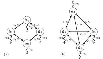
II.1 Circular configuration
The Hamiltonian of a four-mode bosonic system in the circular configuration depicted in Fig. 1(a) takes the following form :
| (1) | |||||
where () for denotes the annihilation (creation) operator of the th mode, () is the linear (nonlinear) coupling strength between the modes [26]. Symbol H.c. replaces the Hermitian-conjugated terms. Damping or amplification of mode is described by the damping (amplification) rate and the corresponding Langevin stochastic operator forces, and that occur in the dynamical Heisenberg-Langevin equations written below in Eq. (2). The Langevin stochastic operator forces are assumed to have the Markovian and Gaussian properties specific to the damping and amplification processes [25]. Their presence in the Heisenberg-Langevin equations guarantees the fulfillment of the field-operator commutation relations. Moreover the properties of the Langevin stochastic operator forces are related to the damping (amplification) rates via the fluctuation-dissipation theorems [10, 11].
The Heisenberg-Langevin equations corresponding to the Hamiltonian in Eq. (1) are written in the form:
| (2) |
where the vectors of field operators and of the Langevin operator forces are given as and . The dynamical matrix introduced in Eq. (2) is derived in the form
| (7) |
The submatrices , , and occurring in Eq. (7) are defined as:
| (12) |
and stands for the damping or amplification rate of the mode .
Applying the conditions
| (13) |
in the dynamical matrix in Eq. (7), we reveal its eigenvalues :
| (14) |
The corresponding eigenvectors are derived as follows:
| (15) |
where , , and .
If then and also . We note that the eigenvalues and share also their imaginary parts, which is important for the observation of -symmetric-like dynamics in a suitable interaction frame [27]. Provided that the system initial conditions are chosen such that only the eigenvalues and determine its dynamics, we observe a second-order QEP. This QEP changes into a QHP with second-order ED and DD when the matrix is analyzed. The condition transforms into the formula
| (16) |
for an ellipse in the parameter space that identifies the positions of QHPs. Real parts of two eigenvalues , , that form QHPs are plotted in this space in Fig. 2(a).
(a) 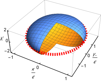
(b) 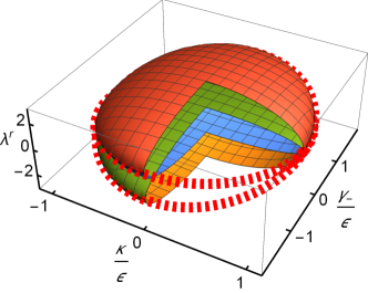
The diagonalized dynamical matrix is obtained with the help of the eigenvalues and eigenvectors given in Eqs. (14) and (15), respectively, and the eigenvalues and the eigenvectors of the matrix :
| (17) |
| (18) |
where . Details can be found in Appendix of Ref. [8]. In the basis with the diagonal dynamical matrix , the system dynamics is described by the new field operators . If the initial conditions allow to describe the complete system dynamics in terms of the field operators , , , and with equal damping or amplification rate then the first- and second-order FOMs exhibit in their dynamics QEPs and QHPs as summarized in Tab. 1.
| Moments | Moment | Genuine and induced QHPs | Genuine QHPs | |||||
| deg. | Partial | Partial | Partial | Partial | ||||
| QDP x | QDP x | QDP x | QDP x | |||||
| QEP deg. | QEP deg. | QEP deg. | QEP deg. | |||||
| , | 1 | 1x2 | 2x2 | 1x2 | 2x2 | |||
| , | 1 | 1x2 | 1x2 | |||||
| , | 2 | 2x4 | 4x4 | 1x4 | 1x4 | |||
| 2 | + | |||||||
| 2 | ||||||||
| , | 1 | 1x4 | 1x3 | 2x3 | ||||
| 2 | ||||||||
| , | 1 | 1x4 | 1x3 | |||||
| 2 | ||||||||
II.2 Tetrahedral configuration
In the tetrahedral configuration depicted in Fig. 1(b), the Hamiltonian of four-mode bosonic system attains the form:
| (19) | |||||
The Heisenberg-Langevin equations corresponding to the Hamiltonian are derived in the form:
| (20) |
using the following dynamical matrix :
| (25) |
In seeking QEPs, we assume equal damping and/or amplification rates of modes 1 and 2, and also of modes 3 and 4:
| (26) |
We note that, due to the symmetry, identical results are obtained when assuming equal damping and/or amplification rates of modes 1 and 3 and also of modes 2 and 4 [compare Eq. (13)].
Under these conditions, diagonalization of the dynamical matrix in Eq. (25) leaves us with the following eigenvalues:
| (27) |
The corresponding eigenvectors are written as:
| (28) |
and , , and .
Provided that , we have and as . As the imaginary parts of eigenvalues differ from those of , the system can exhibit only the non-conventional -symmetric dynamics: If the system initial conditions are such that only the eigenvalues and suffice in describing its dynamics, we observe a second-order QEP for the dynamical matrix . As the eigenvalues in Eq. (27) show the linear dependence on , the diabolical second-order degeneracy of the dynamical matrix , originating in the form of the eigenvalues in Eq. (14), is not observed in the tetrahedral configuration. Instead, for , we find one second-order QEP for and another second-order QEP for . These QEPs occur at the positions described in Eq. (16) in the parameter space . Real parts of four eigenvalues for that build two QEPs are drawn in this space in Fig. 2(b).
In the basis with the diagonal dynamical matrix , the system dynamics is described by the new field operators . The corresponding eigenvalues and eigenvectors are discussed in general in Appendix of Ref. [8]. The first- and second-order FOMs exhibit in their dynamics QEPs and QHPs that are summarized in Tab. 2.
| Moments | Moment | Genuine and induced QHPs | Genuine QHPs | |||||
| deg. | Partial | Partial | Partial | Partial | ||||
| QDP x | QDP x | QDP x | QDP x | |||||
| QEP deg. | QEP deg. | QEP deg. | QEP deg. | |||||
| , | 1 | 1x2 | 1x2 | 1x2 | 1x2 | |||
| , | 1 | 1x2 | 1x2 | 1x2 | 1x2 | |||
| , | 2 | 2x4 | 2x4 | 1x4 | 1x4 | |||
| , | 2 | |||||||
| , | 1 | 1x4 | 1x4 | 1x3 | 1x3 | |||
| 2 | ||||||||
| , | 1 | 1x4 | 1x4 | 1x3 | 1x3 | |||
| 2 | ||||||||
III Concatenated bosonic systems with unidirectional coupling: Higher-order quantum exceptional points on demand
The previous analysis of the bosonic systems with up to five modes in their linear, circular, tetrahedron, and pyramid configurations revealed only the inherited QEPs and QHPs with second- and third-order EDs. Here, we extend our analysis to more general non-Hermitian Hamiltonians that involve unidirectional coupling between the modes. Whereas the non-Hermiticity of the above discussed systems is given solely by the presence of damping and/or amplification, the Hamiltonians with unidirectional coupling are non-Hermitian per se, while damping and amplification make them even more non-Hermitian. Despite their non-Hermiticity, they have direct physical implementations based upon counter-directional field propagation and mutual scattering [12, 13]. Moreover, it has been shown in Ref. [28] that exponential improvement of measurement precision can be reached in QEPs in systems with unidirectional coupling.
It was shown in Refs. [12, 13] that using a specific unidirectional coupling of two field modes belonging to different -symmetric systems with QEPs, the combined system exhibits a QEP with ED given as the sum of those of the constituting systems. This opens the door for observing inherited QEPs with EDs of orders higher than three.
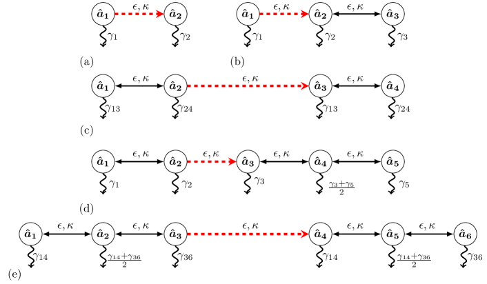
To demonstrate the method, let us consider two bosonic modes that are unidirectionally coupled via the matrix defined in Eq. (12) [see the scheme in Fig. 3(a)].
As we demonstrate below, this unidirectional coupling creates a QEP. The corresponding Heisenberg-Langevin equations take the form
| (29) |
where the vectors of field operators and of the Langevin operator forces are given as and . The properties of the Langevin operator forces are described in detail below, i.e. in Eq. (124).
The dynamical matrix introduced in Eq. (29) and corresponding to unidirectional coupling of modes is written as
| (32) |
using the damping or amplification submatrices , , defined in Eq. (12). The eigenvalues and eigenvectors of the matrix are determined as
| (33) |
and
| (34) |
Provided that
| (35) |
we have together with , and so we observe the creation of a QEP with second-order ED. This means that the matrix obtained after inserting the submatrices , , and into Eq. (32) exhibits a QHP with second-order ED and DD. It is worth noting that these QHPs occur independently of the values of the coupling strengths and , in strike difference to the QHPs found in the two-mode bosonic system analyzed in Sec. II of Ref. [8].
In the next step we demonstrate the increase of the order of ED of a QEP by considering a single-mode bosonic system unidirectionally coupled to a two-mode bosonic system with a QEP [see the scheme in Fig. 4(b)]. The dynamical matrix of the concatenated system is given as:
| (39) |
Provided that
| (40) |
we arrive at the eigenvalues:
| (41) |
and the corresponding eigenvectors:
| (42) |
where and . If , i.e., when the condition
| (43) |
for the constituting two-mode system is fulfilled, we have , and . This identifies a QEP with third-order ED that emerged from the original QEP with second-order ED. This means that we have a QHP with third-order ED and second-order DD in the matrix . Introducing the new field operators, in which the dynamical matrix attains its diagonal form, we reveal QEPs and QHPs and their degeneracies appropriate to the dynamics of the first- and second-order FOMs. They can be found in Tab. 3 derived for a general -mode bosonic system exhibiting an inherited QHP with th-order ED and second-order DD for . We note that Tab. 3 applies also to the bosonic systems analyzed below.
| Moments | Moment | Genuine and induced QHPs | Genuine QHPs | |||||
| deg. | Partial | Partial | Partial | Partial | ||||
| QDP x | QDP x | QDP x | QDP x | |||||
| QEP deg. | QEP deg. | QEP deg. | QEP deg. | |||||
| 1 | 1xn | 2xn | 1xn | 2xn | ||||
| 1 | 1xn | 1xn | ||||||
| , | 2 | 2x | 4x | 1x | 1x | |||
| 2 | + | |||||||
| 2 | ||||||||
| , | 1 | 1x | 1x | 2x | ||||
| , | 2 | |||||||
| 2 | ||||||||
| , | 1 | 1x | 1x | |||||
| , | 2 | |||||||
| 2 | ||||||||
Now, we construct four-, five-, and six-mode bosonic systems by concatenating the two- and three-mode systems with second- and third-order QEPs analyzed in Secs. II and III of Ref. [8]. We begin with combining two two-mode systems [see the scheme in Fig. 4(c)] whose dynamical matrices denoted as and are defined as follows [compare Eq. (3) of part I of the paper]:
| (46) |
The joint dynamical matrix , defined as
| (49) |
includes unidirectional coupling between modes 2 and 3 described by the submatrix :
| (51) |
Assuming
| (52) |
we reveal the eigenvalues of the matrix as follows:
| (53) |
using and . For , a QEP with fourth-order ED is found at the positions in the parameter space given by Eq. (43), i.e., where the constituting two-mode systems form QEPs with second-order EDs. The fourth-order QEP implies a QHP with fourth-order ED and second-order DD of the matrix . It is worth noting that the additional unidirectional coupling of modes 1 and 4, i.e. when , does not change the eigenvalues in Eq. (52) and also preserves the structure of eigenvectors with the discussed QEPs and QHPs.
The unidirectional coupling of the two- and three-mode systems allows to observe a QEP with fifth-order ED [for the configuration, see Fig. 4(d)]. The corresponding dynamical matrix combines the two-mode dynamical matrix in Eq. (46) and the three-mode dynamical matrix [compare Eq. (19) in [8]],
| (57) |
The matrix is expressed as
| (60) |
assuming the unidirectional coupling between modes 2 and 3:
| (62) |
Provided that
| (63) |
we determine the eigenvalues of the matrix as follows:
| (64) |
where , , , and . Provided that and , we find a QEP with fifth-order ED. These conditions define the positions, which are specified in Eq. (43) and the following one:
| (65) |
Both conditions have to be fulfilled simultaneously, which results in the following condition
| (66) |
Thus, we reveal the QHPs of the matrix under the conditions, given in Eqs. (63) and (66), observed in the space at the positions obeying Eq. (43).
The last analyzed system is created by unidirectional combining of two three-mode systems with identical parameters in the configuration shown in Fig. 4(e). Its dynamical matrix, denoted as , is composed of the two three-mode dynamical matrices from Eq. (57) and the coupling matrix ,
| (67) |
It is expressed in the form
| (70) |
in which we assume:
| (72) |
The eigenvalues of the matrix are determined in the form:
| (73) |
where and . It holds at the positions in the parameter space that fulfil the condition
| (74) |
At these positions we have six identical eigenvalues in Eq. (73). They indicate a QEP with sixth-order ED that implies a QHP of sixth-order ED and second-order DD in the dynamical matrix .
In the last three analyzed systems, explicit forms for the eigenvectors of the dynamical matrices , , and were not analyzed because of their complexity. Instead, these dynamical matrices were diagonalized under the conditions at which QEPs are expected and the transformed matrices in the Jordan form with unit elements at the upper diagonal confirmed the presence of QEPs.
The considered forms of unidirectional coupling matrices , , and can be replaced by those connecting different pairs of modes in the constituting systems. This replacement does not change the eigenvalues as well as the degeneracies of the eigenvectors that give rise to the observed QEPs and QHPs. We note that the form of eigenvectors depends on which pairs of modes are unidirectionally coupled. We can even include unidirectional coupling of several pairs of modes in the constituting systems and this property still holds. The only requirement is that all couplings point out from one subsystem to the other subsystem.
We note that there exist alternative ways to realize unidirectional coupling between the constituting bosonic systems. Contrary to the considered unidirectional coupling that is described directly via the dynamical matrices, we may consider an alternative form of unidirectional coupling characterized by the Hamiltonians
| (75) | |||||
| (76) |
They result in the system dynamics similar to that discussed above and lead to the eigenvalues and eigenvectors with characteristic EDs and DDs. This improves the feasibility of practical realizations of such concatenated bosonic systems with higher-order QEPs and QHPs based on unidirectional coupling.
The method is general, allowing for concatenating simple bosonic systems into more complex ones that keep QEPs and QHPs of the original systems using unidirectional coupling of different kinds. Combing the analyzed bosonic systems with second- and third-order EDs together, bosonic systems with arbitrary-order EDs can be achieved.
IV Unidirectional coupling and its applicability
In this section, we reveal characteristic features of the bosonic systems with unidirectional coupling and specify the conditions of their applicability. We consider the simplest two-mode bosonic system with unidirectional coupling whose dynamics is described by the Heisenberg-Langevin equations written in Eq. (29) with the dynamical matrix given in Eq. (32). We assume the most typical configuration of -symmetric systems in which mode 1 is damped and mode 2 is amplified:
| (77) |
The corresponding Langevin fluctuating operator forces embedded in the vector are modelled by two independent quantum random Gaussian processes [29, 30, 31]. This results in the following correlation functions:
| (78) |
The remaining second-order correlation functions are zero. Symbol stands for the Dirac function.
The solution to the stochastic linear differential operator equations in Eq. (29) is expressed in the form
| (79) |
using the evolution matrix defined as
| (80) |
The fluctuating operator forces introduced in Eq. (79) are determined along the formula
| (81) |
It implies the following formula for their second-order correlation functions,
| (82) | |||||
The solution in Eq. (79) can be recast into a simpler form written for the annihilation operators and :
| (91) |
The elements of the matrices and are defined as and for , and we also have for .
Using the eigenvalues and eigenvectors written in Eqs. (17), (18), (33), and (34), we arrive at the formulas specific to our model:
| (97) | |||
| (100) | |||
| (105) | |||
| (110) | |||
| (111) |
where , , and using the hyperbolic sinus function.
To check consistency of the model with unidirectional coupling, we determine the mean values of equal time field-operators commutation relations. Compared to the usual canonical commutation relations , , and for , the following two relations are found:
| (112) |
where and . For short times assuming we have and . Thus, we additionally require and . As we usually assume in -symmetric systems that , we are left with the following conditions for applicability of the model with unidirectional coupling:
| (113) |
The form of the commutation relations given in Eq. (112) and the ensuing restricted validity of the model poses the question about possible corrections of the model using suitable properties of the reservoir Langevin operator forces. Similarly as it is done when damping and amplification are introduced into the Heisenberg equations (the Wigner–Weisskopf model of damping, see Ref. [11]). However, as discussed in detail in Appendix A, this approach is not successful.
Also, in Appendix B the properties of the modes are analyzed in the framework of the Gaussian states, their nonclassicality depths and logarithmic negativity are determined. These results point out at specific properties of the two-mode bosonic system with unidirectional coupling applicable only under the conditions given in Eq. (113).
These results lead us to the conclusion that the method for concatenating simpler bosonic systems with QEPs to arrive at QEPs with higher-order ED has limitations. The question how to obtain higher-order inherited QEPs in bosonic systems without these limitations is open.
V Numerical identification of exceptional points and their degeneracies
When an analyzed system is more complex and we do not succeed in revealing its eigenvalues and eigenvectors analytically, we can apply two different numerical approaches to arrive at the orders of exceptional degeneracies. We demonstrate both approaches analytically using the simplest two-mode systems with the usual and unidirectional couplings.
V.1 Jordan canonical form of a general matrix
The Jordan form of a matrix contains nonzero elements on the diagonal and also the nearest upper diagonal. It has the dimension of the matrix . Some elements at the nearest upper diagonal equal one if the matrix is non-diagonalizable. The neighbor elements equal to one form groups. The number of elements in a given group gives the order of ED (equal to the number of elements + 1) related to the corresponding eigenvalue.
For example and considering the dynamical matrix , given in Eq. (46), belonging to the two-mode bosonic system with usual coupling under the condition , i.e., where a second-order QEP occurs, the Jordan form and the corresponding similarity transformation such that
| (114) |
take the form:
| (115) |
In Eq. (115), the element (1,2) of the matrix , equal to 1, identifies a second-order QEP.
Similarly, when analyzing the two-mode bosonic system with unidirectional coupling and the dynamical matrix , written in Eq. (32), under the condition guaranteeing the existence of a second-order QEP, we arrive at:
| (116) |
V.2 Perturbation of a dynamical matrix
The second approach is based upon introducing a suitable small perturbation of a dynamical matrix that can remove both EDs and DDs. In this approach, the eigenvalues of the perturbed dynamical matrix are determined and the degeneracies are removed as the degenerated eigenvalues split and then gradually diverge with the increasing perturbation. Perturbation can also be used for characterizing ED [32, 33, 34].
Identifying EDs, we demonstrate different kinds of the influence of perturbation on the eigenvalues of the matrix considering the two-mode systems with the usual and unidirectional couplings and different positions of the perturbation inside the matrix . Specifically, we demonstrate splitting of the eigenvalues in their real and/or imaginary parts and splitting proportional to and when a QEP with second-order ED is disturbed. We quantify the strength of the perturbation by the overlap of the normalized eigenvectors and that become gradually distinguishable as the perturbation increases
| (117) |
and symbol stands for the scalar product of complex vectors.
-
1.
A two-mode system with usual coupling and described by the perturbed dynamical matrix
(118) The eigenvalues and the corresponding eigenvectors take, respectively, the form:
(119) and
(120) -
2.
A two-mode system with usual coupling and described by the perturbed dynamical matrix
(121) The eigenvalues and the corresponding eigenvectors are derived, respectively, as follows:
(122) and
(123) -
3.
A two-mode system with unidirectional coupling and described by the perturbed dynamical matrix
(124) The eigenvalues and the corresponding eigenvectors are attained, respectively, in the form:
(125) and
(126)
(a) 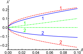
(b) 
(c) 
The real and imaginary parts of the eigenvalues , , from Eqs. (119), (122), and (125) are plotted in Figs. 4(a,b) as they depend on the perturbation . The perturbation in general disturbs more strongly the system with the usual coupling, as it is apparent both from the graphs of the eigenvalues and the overlap of eigenvectors shown in Fig. 4(c).
In the above-discussed cases, the second-order DD present in both two-mode systems was not modified by the perturbation because of the structure of these systems. However, suitable positioning of the perturbation inside a dynamical matrix may also result in revealing the DDs. As the DD is embedded in the matrix given in Eq. (12), the perturbation has to affect this matrix. We consider two kinds of perturbation in the two-mode system with the dynamical matrix : The first one splits all eigenvalues , , in their real parts, whereas the second one distinguishes two eigenvalues in their real parts and the remaining two eigenvalues in their imaginary parts. We note that the perturbation primarily modifies the eigenvalues of the matrix , which removes the DD. Secondarily, as the eigenvalues of determined for nonzero differ from those valid for , the conditions for having a QEP of the matrix change and the original setting of the system parameters for a QEP is lost and so also the corresponding ED is lost.
-
1.
A two-mode system with usual coupling and described by the dynamical matrix where
(127) The eigenvalues and the corresponding eigenvectors of matrix are written, respectively, as:
(128) and
(129) -
2.
A two-mode system with usual coupling and described by the dynamical matrix where
(130) The eigenvalues and the corresponding eigenvectors of matrix are obtained, respectively, as:
(131) and
(132)
The looked for eigenvalues and eigenvectors are then reached using the eigenvalues and eigenvectors of the matrix written in Eq. (46):
| (133) |
and
| (134) |
where and . The real and imaginary parts of the eigenvalues , , of the matrix are plotted in Fig. LABEL:fig5.
(a) 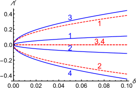
(b) 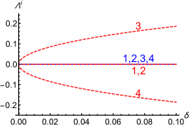
Finally, we mention a specific case of the perturbation that removes DD but keeps one from the two originally diabolically-degenerated QEPs present in the system. The dynamical matrix of the two-mode bosonic system with usual coupling is perturbed in the following way:
| (137) |
The eigenvalues of the dynamical matrix in Eq. (137) are derived in the form:
| (138) |
The corresponding eigenvectors are expressed as follows:
| (140) | |||||
| (142) |
According to Eqs. (138) and (142), we observe a single QEP with second-order ED for and . This contrasts with the observation of a QEP with second-order ED and also second-order DD for and .
VI Higher-order hybrid points revealed by field-operator moments
In the last section, we derive general formulas that give us the orders of EDs and DDs of QHPs that occur in the dynamics of higher-order FOMs. We note that the structure of higher-order FOM spaces mapped onto suitable lattices and its influence to system’s properties has been analyzed in detail in Ref. [35] for two- and three-mode bosonic systems.
Let us consider a bosonic system composed on modes and described by an appropriate quadratic non-Hermitian Hamiltonian. Such a system is described by the annihilation and creation operators, and the dynamical matrix of its Heisenberg-Langevin equations has eigenvalues. Let us fix a position in the system parameter space. After diagonalization of the dynamical matrix , we identify the eigenvalues with different eigenvectors and count their degeneration numbers according to the number of coalescing eigenvectors (from the original maximal Hilbert space). Denoting the number of such eigenvalues by , we have
| (143) |
We assign, to any eigenvalue , an operator vector that encompasses the diagonalized field operators and () that are associated with the coalescing vectors of this eigenvalue.
Now we consider the dynamics of th-order FOMs. These th-order FOMs can formally be expressed in their general form using the above-defined operator vectors as , where the nonnegative integers obey . The vector defined as then points out at a possible QHP with the complex eigenfrequency given as
| (144) |
The degrees of ED and of DD of this QHP are given by the following formulas:
| (145) | |||||
| (146) |
The number of such QHPs observed for the th-order FOMs (see the fourth columns of Tabs. I—VI in Ref. [8]) is determined using the combination number as:
| (147) |
Similar formula also gives the number of different th-order FOMs written in the operators and for :
| (148) |
These FOMs are explicitly written in the third columns of Tabs. I—VI in Ref. [8]. Also, the number of different th-order FOMs written in the operators and and belonging to a fixed is expressed as:
| (149) |
To demonstrate the general approach and formulas, we apply them to the four-mode bosonic system in the circular configuration analyzed in Sec. II in the regime of nonconventional PT-symmetric dynamics. Its first- and second-order FOMs and the revealed QHPs with their degeneracies are given in Tab. 1. The general approach results in Tab. 4 that allows to easily derive the content of Tab. 1: Two lines belonging to are obtained assuming and . For the entries to Tab. 1 are in turn generated assuming , , and . The orders of the corresponding EDs and DDs are derived using Eqs. (145) and (146), respectively.
| 1 | |||
| 1 | |||
| 1 | |||
| 1 | |||
| 2 | |||
| 2 | |||
These results can be used for detailed discussions of genuine and induced QHPs and their degeneracies for FOMs of arbitrary orders and considering different systems with their specific inherited QHPs observed in the dynamics of field operators governed by the Heisenberg-Langevin equations. The occurrence of a QHP with th ED and second-order DD in the dynamics of th-order FOMs in a bosonic system with an inherited QHP with th-order ED and second-order DD is probably the most valuable result.
VII Conclusions
We have continued the analysis of the dynamics of simple bosonic systems described by quadratic non-Hermitian Hamiltonians from the point of view of the occurrence of quantum exceptional, diabolical, and hybrid points. We have revealed the bosonic systems exhibiting nonconventional -symmetric dynamics characterized by the observation of quantum exceptional and hybrid points only in certain subspace(s) of the whole system Liouville space. We have identified such nonconventional second-order inherited quantum exceptional and hybrid points in four-mode bosonic systems.
Applying the method of concatenating simple bosonic systems via unidirectional coupling, we have found the conditions for the observation of up to sixth-order inherited quantum exceptional and hybrid points. However, by analyzing the behavior of the two-mode bosonic system with unidirectional coupling we have shown that the bosonic systems with unidirectional coupling are applicable only for short times in which they ensure physically consistent behavior. In short times, more complex bosonic systems with diverse structures and arbitrary-order exceptional degeneracies can be built by concatenating simple bosonic systems via unidirectional coupling of several types. Nevertheless, tailoring the properties of the Langevin operator stochastic forces in systems with unidirectional coupling does not enable extending their applicability to arbitrary times, in contrast to how the damping and amplification are consistently described.
Using analytical formulas for two-mode bosonic systems we have elucidated the operation of two numerical methods for the identification of quantum exceptional points and their degeneracies. These include: (1) the transformation of a dynamical matrix into its Jordan form and (2) the introduction of a suitable perturbation into the dynamical matrix and its subsequent eigenvalue analysis.
The exceptional and diabolical degeneracies of inherited quantum hybrid points have been used to derive higher-order degeneracies observed in the dynamics of higher-order field-operator moments. The quantum exceptional and hybrid points of second-order field-operator moments have been summarized in tables that evidence a rich dynamics of the field-operator moments.
Numbers of genuine and induced quantum hybrid points and their exceptional and diabolical degeneracies have been expressed as they depend on the order of the field-operator moments in the general form using parameters of the inherited quantum exceptional and hybrid points and their degeneracies.
This analysis considerably broadens the investigations of bosonic systems with -symmetry exhibiting correct physical behavior, though it does not reveal bosonic systems with higher-order exceptional and hybrid singularities found for arbitrarily long times. The bosonic systems with unidirectional coupling enable generating higher-order exceptional and hybrid points only in their short-time dynamics. The systems with nonconventional -symmetric dynamics exhibit only low- (second-) order exceptional and hybrid degeneracies, similarly as their counterparts analyzed in Ref. [8]. This analysis together with that in Ref. [8] show that the observation of higher-order exceptional and hybrid singularities in real, i.e. physically well-behaved, bosonic systems at arbitrary times is challenging.
VIII Acknowledgements
The authors thank Ievgen I. Arkhipov for useful discussions. J.P. and K.T. acknowledge support by the project OP JAC CZ.02.01.01/00/22_008/0004596 of the Ministry of Education, Youth, and Sports of the Czech Republic. A.K.-K., G.Ch., and A.M. were supported by the Polish National Science Centre (NCN) under the Maestro Grant No. DEC-2019/34/A/ST2/00081.
Appendix A Two-mode system with unidirectional coupling and relevant reservoir properties
Considering the approach outlined in Ref. [36], we construct the matrix of the stochastic Langevin operator forces such that the bosonic commutation relations of the field operators are obeyed for an arbitrary time .
First, we note that the additional, unwanted, terms in the commutation relations in Eq. (112) disappear when we replace the correlation matrix of the fluctuating operator forces given in Eq. (100) by the matrix with the constituting submatrices:
| (152) | |||||
| (155) |
where the functions and are defined below Eq. (112).
Inverting Eq. (82) (for details, see Eq. (18) in Ref. [36]) we obtain the correlation matrix of the Langevin operator forces as follows:
| (160) | |||||
where ; .
However, the correlation matrix does not represent a physical reservoir, as it has a negative eigenvalue. This can be even analytically confirmed considering . In this case, the eigenvalues are obtained as:
| (161) |
This means in general that there does not exist a physical reservoir with properties such that the model with unidirectional coupling could be applied for an arbitrary time .
Appendix B Statistical properties of a two-mode bosonic system with unidirectional coupling
We consider modes 1 and 2 being in their initial coherent states and , respectively. The modes evolution described in Eq. (LABEL:52) maintains the state Gaussian form described by the following normal characteristic function [11, 37, 7]:
where symbol c.c. replaces the complex conjugated terms. The functions , , and are given as:
| (163) |
and for an arbitrary operator . The functions , , , and are defined below Eqs. (112) and (160), while the complex modes amplitudes and are derived from their initial values along the relations
| (170) |
where the matrices and are given in Eq. (97).
Using the formulas in Eq. (163), the nonclassicality depth of mode 2 [38], determined as
| (171) |
is vanishing, which means the classical behavior of the marginal field in mode 2. Also the marginal field in mode 1 stays classical, as we have .
We quantify the entanglement between the fields in modes 1 and 2 by the logarithmic negativity [39] determined from the simplectic eigenvalues of the partially-transposed symmetrically-ordered covariance matrix [40], as given by:
| (174) | |||||
| (177) | |||||
| (180) |
where stands for the two-dimensional identity matrix. Determining two invariants and of the matrix , the simplectic eigenvalues are expressed as [40]:
| (181) |
The logarithmic negativity is then determined along the formula
| (182) |
As the model is applicable only for short times , fulfilling the conditions in Eq. (113), we derive the logarithmic negativity using the Taylor expansion in to first order:
| (183) |
The formula (183) predicts nonzero negativity for short times despite the fact that mode 1 remains in a coherent state. If then and mode 1 remains in the vacuum state. However, this state cannot be entangled with mode 2, as the formula (183) for negativity predicts. This is another manifestation of the limited applicability of the studied model with unidirectional propagation.
References
- Chen et al. [2017] W. Chen, Ş. K. Özdemir, G. Zhao, J. Wiersig, and L. Yang, Exceptional points enhance sensing in an optical microcavity, Nature (London) 548, 192 (2017).
- Liu et al. [2016] Z.-P. Liu, J. Zhang, S. K. Özdemir, B. Peng, H. Jing, X.-Y. Lü, C.-W. Li, L. Yang, F. Nori, and Y.-X. Liu, Metrology with -symmetric cavities: Enhanced sensitivity near the -phase transition, Phys. Rev. Lett. 117, 110802 (2016).
- Feng et al. [2017] L. Feng, R. El-Ganainy, and L. Ge, Non-Hermitian physics and symmetry, Nat. Photon. 11, 752 (2017).
- El-Ganainy et al. [2019] R. El-Ganainy, M. Khajavikhan, S. Rotter, D. N. Christodoulides, and Ş. K. Özdemir, Non-Hermitian physics and symmetry, Commun. Phys. 2, 1 (2019).
- Parto et al. [2021] M. Parto, Y. G. N. Liu, B. Bahari, M. Khajavikhan, and D. N. Christodoulides, Non-Hermitian and topological photonics: Optics at an exceptional point, Nanophotonics 10, 403 (2021).
- Peřina Jr. and Lukš [2019] J. Peřina Jr. and A. Lukš, Quantum behavior of a -symmetric two-mode system with cross-Kerr nonlinearity, Symmetry 11, 1020 (2019).
- Peřina Jr. et al. [2019] J. Peřina Jr., A. Lukš, J. K. Kalaga, W. Leoński, and A. Miranowicz, Nonclassical light at exceptional points of a quantum -symmetric two-mode system, Phys. Rev. A 100, 053820 (2019).
- Thapliyal et al. [2024] K. Thapliyal, J. Peřina Jr., G. Chimczak, A. Kowalewska-Kudłaszyk, and A. Miranowicz, Multiple quantum exceptional, diabolical, and hybrid points in multimode bosonic systems: I. Inherited and genuine singularities, arxiv (2024).
- Peřina Jr. [1995] J. Peřina Jr., On the equivalence of some projection operator techniques, Physica A 214, 309 (1995).
- Vogel and Welsch [2006] W. Vogel and D. G. Welsch, Quantum Optics, 3rd ed. (Wiley-VCH, Weinheim, 2006).
- Peřina [1991] J. Peřina, Quantum Statistics of Linear and Nonlinear Optical Phenomena (Kluwer, Dordrecht, 1991).
- Zhong et al. [2020] Q. Zhong, J. Kou, Ş. Özdemir, and R. El-Ganainy, Hierarchical construction of higher-order exceptional points, Phys. Rev. Lett. 125, 203602 (2020).
- Wiersig [2022a] J. Wiersig, Revisiting the hierarchical construction of higher-order exceptional points, Phys. Rev. A 106, 063526 (2022a).
- Wang et al. [2019] S. Wang, B. Hou, W. Lu, Y. Chen, Z. Zhang, and C. T. Chan, Arbitrary order exceptional point induced by photonic spin–orbit interaction in coupled resonators, Nature Commun. 10, 832 (2019).
- Jing et al. [2017] H. Jing, S. K. Özdemir, H. Lu, and F. Nori, High-order exceptional points in optomechanics, Sci. Rep. 7, 3386 (2017).
- Zhang and You [2019] G.-Q. Zhang and J. You, Higher-order exceptional point in a cavity magnonics system, Phys. Rev. B 99, 054404 (2019).
- Graefe et al. [2008] E. M. Graefe, U. Günther, H. J. Korsch, and A. E. Niederle, A non-Hermitian symmetric Bose–Hubbard model: Eigenvalue rings from unfolding higher-order exceptional points, J. Phys. A: Math. Theor. 41, 255206 (2008).
- Teimourpour et al. [2014] M. Teimourpour, R. El-Ganainy, A. Eisfeld, A. Szameit, and D. N. Christodoulides, Light transport in pt-invariant photonic structures with hidden symmetries, Phys. Rev. A 90, 053817 (2014).
- Znojil [2018] M. Znojil, Complex symmetric Hamiltonians and exceptional points of order four and five, Phys. Rev. A 98, 032109 (2018).
- Mandal and Bergholtz [2021] I. Mandal and E. J. Bergholtz, Symmetry and higher-order exceptional points, Phys. Rev. Lett. 127, 186601 (2021).
- Delplace et al. [2021] P. Delplace, T. Yoshida, and Y. Hatsugai, Symmetry-protected multifold exceptional points and their topological characterization, Phys. Rev. Lett. 127, 186602 (2021).
- Zhong et al. [2018] Q. Zhong, D. N. Christodoulides, M. Khajavikhan, K. Makris, and R. El-Ganainy, Power-law scaling of extreme dynamics near higher-order exceptional points, Phys. Rev. A 97, 020105 (2018).
- Hodaei et al. [2017] H. Hodaei, A. U. Hassan, S. Wittek, H. Garcia-Gracia, R. El-Ganainy, D. N. Christodoulides, and M. Khajavikhan, Enhanced sensitivity at higher-order exceptional points, Nature (London) 548, 187 (2017).
- Li et al. [2023] Z.-Z. Li, W. Chen, M. Abbasi, K. W. Murch, and K. B. Whaley, Speeding up entanglement generation by proximity to higher-order exceptional points, Phys. Rev. Lett. 131, 100202 (2023).
- Peřina Jr. et al. [2022] J. Peřina Jr., A. Miranowicz, G. Chimczak, and A. Kowalewska-Kudłaszyk, Quantum Liouvillian exceptional and diabolical points for bosonic fields with quadratic Hamiltonians: The Heisenberg-Langevin equation approach, Quantum 6, 883 (2022).
- Boyd [2003] R. W. Boyd, Nonlinear Optics, 2nd edition (Academic Press, New York, 2003).
- Chimczak et al. [2023] G. Chimczak, A. Kowalewska-Kudłaszyk, E. Lange, K. Bartkiewicz, and J. Peřina Jr., The effect of thermal photons on exceptional points in coupled resonators, Sci. Rep. 13, 5859 (2023).
- McDonald and Clerk [2020] A. McDonald and A. A. Clerk, Exponentially-enhanced quantum sensing with non-hermitian lattice dynamics, Nature Communications 11, 5382 (2020).
- Meystre and Sargent III [2007] P. Meystre and M. Sargent III, Elements of Quantum Optics, 4nd edition (Springer, Berlin, 2007).
- Agarwal and Qu [2012] G. S. Agarwal and K. Qu, Spontaneous generation of photons in transmission of quantum fields in -symmetric optical systems, Phys. Rev. A 85, 031802(R) (2012).
- Peřinová et al. [2019] V. Peřinová, A. Lukš, and J. Křepelka, Quantum description of a -symmetric nonlinear directional coupler, J. Opt. Soc. Am. B 36, 855 (2019).
- Znojil [2019] M. Znojil, Unitarity corridors to exceptional points, Phys. Rev. A 100, 032124 (2019).
- Wiersig [2022b] J. Wiersig, Response strengths of open systems at exceptional points, Phys. Rev. Res. 4, 023121 (2022b).
- Wiersig [2022c] J. Wiersig, Distance between exceptional points and diabolic points and its implication for the response strength of non-Hermitian systems, Phys. Rev. Res. 4, 033179 (2022c).
- Arkhipov et al. [2023] I. I. Arkhipov, A. Miranowicz, F. Nori, S. K. Özdemir, and F. Minganti, Fully solvable finite simplex lattices with open boundaries in arbitrary dimensions, Phys. Rev. Res. 5, 043092 (2023).
- Peřina Jr. et al. [2023] J. Peřina Jr., A. Miranowicz, J. K. Kalaga, and W. Leoňski, Unavoidability of nonclassicality loss in -symmetric systems, Phys. Rev. A 108, 033512 (2023).
- Peřina Jr. and Peřina [2000] J. Peřina Jr. and J. Peřina, Quantum statistics of nonlinear optical couplers, in Progress in Optics, Vol. 41, edited by E. Wolf (Elsevier, Amsterdam, 2000) pp. 361—419.
- Lee [1991] C. T. Lee, Measure of the nonclassicality of nonclassical states, Phys. Rev. A 44, R2775 (1991).
- Hill and Wootters [1997] S. Hill and W. K. Wootters, Computable entanglement, Phys. Rev. Lett. 78, 5022 (1997).
- Adesso and Illuminati [2007] G. Adesso and F. Illuminati, Entanglement in continuous variable systems: Recent advances and current perspectives, J. Phys. A: Math. Theor. 40, 7821 (2007).