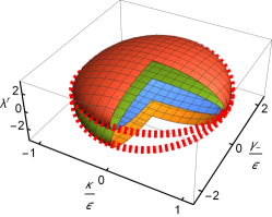
Multiple quantum exceptional, diabolical, and hybrid points in multimode bosonic systems: I. Inherited and genuine singularities

Kishore Thapliyal Email: kishore.thapliyal@upol.cz Affiliation: Joint Laboratory of Optics, Faculty of Science, Palacký University, Czech Republic, 17. listopadu 12, 771 46 Olomouc, Czech Republic    Jan Peřina Jr Email: jan.perina.jr@upol.cz Affiliation: Joint Laboratory of Optics, Faculty of Science, Palacký University, Czech Republic, 17. listopadu 12, 771 46 Olomouc, Czech Republic    Grzegorz Chimczak Affiliation: Institute of Spintronics and Quantum Information, Faculty of Physics, Adam Mickiewicz University, 61-614 Poznań, Poland    Anna Kowalewska-Kudłaszyk Affiliation: Institute of Spintronics and Quantum Information, Faculty of Physics, Adam Mickiewicz University, 61-614 Poznań, Poland    Adam Miranowicz Affiliation: Institute of Spintronics and Quantum Information, Faculty of Physics, Adam Mickiewicz University, 61-614 Poznań, Poland
Abstract

The existence and degeneracies of quantum exceptional, diabolical, and hybrid (i.e., diabolically degenerated exceptional) singularities of simple bosonic systems composed of up to five modes with damping and/or amplification are analyzed. Their dynamics governed by quadratic non-Hermitian Hamiltonians is followed using the Heisenberg-Langevin equations. Conditions for the observation of inherited quantum hybrid points, observed directly in the dynamics of field operators, having up to third-order exceptional and second-order diabolical degeneracies are revealed. Exceptional and diabolical genuine points and their degeneracies observed in the dynamics of second-order field-operator moments are analyzed. Surprisingly, exceptional degeneracies of only second and third orders are revealed. Nevertheless the analyzed bosonic systems exhibit rich dynamics, also owing to their common second-order diabolical degeneracies.

I Introduction

Non-Hermitian Hamiltonians had been for a long time considered not being suitable for describing real physical systems. This opinion has changed after the seminal work by Bender and Boettcher Bender and Boettcher 1998 who showed that the non-Hermitian Hamiltonians endowed with a parity and time symmetry (𝒫𝒯\mathcal{PT}-symmetry) exhibit real spectra in certain areas of the system parameter space. This leads to the formulation of new area of physics, i.e., non-Hermitian quantum mechanics Bender et al. 2003; Bender 2007; El-Ganainy et al. 2018; Ashida et al. 2020, which has already provided numerous models Mostafazadeh 2003; Mostafazadeh 2004; Mostafazadeh 2010; Znojil 2008; Brody 2014; Bagarello et al. 2016 suitable for describing real quantum systems in many areas of physics. Moreover, non-Hermitian Hamiltonians exhibit new algebraic structures: It has been shown that, for certain values of parameters, there occur spectral degeneracies accompanied by degeneracies of the eigenvectors of a given Hamiltonian. Such points in a system parameter space with exceptional degeneracies (EDs) are called exceptional points (EPs) for which the dimension of the corresponding Hilbert space is reduced. This has interesting physical consequences and leads to new unexpected physical effects. It allows to enhance the precision of measurements of suitable physical quantities Chen et al. 2017; Liu et al. 2016; Feng et al. 2017; El-Ganainy et al. 2019; Parto et al. 2021. It also leads to enhanced nonlinear interactions Peřina Jr. and Lukš 2019; Peřina Jr. et al. 2019. For this reason, 𝒫𝒯\mathcal{PT}-symmetric systems of different kinds have been found appealing in many areas of physics including: optical waveguides Turitsyna et al. 2017; Xu et al. 2018, optical lattices Graefe and Jones 2011; Miri et al. 2012; Ornigotti and Szameit 2014; Shui et al. 2019, spin lasers Drong et al. 2022, optical coupled structures El-Ganainy et al. 2007; Ramezani et al. 2010; Zyablovsky et al. 2014; Ögren et al. 2017; Naikoo et al. 2019, coupled optical microresonators Peng et al. 2014a; Peng et al. 2014b; Liu et al. 2016; Zhou and Chong 2016; Arkhipov et al. 2019; Arkhipov et al. 2020, quantum-electrodynamics circuits (QED) Quijandría et al. 2018, systems with complex potentials Guo et al. 2009, optomechanical systems Tchodimou et al. 2017; Wang et al. 2019, photonics molecules El-Ganainy et al. 2014, among others. Moreover, schemes for engineering properties of EPs have been suggested (see, e.g., Minganti et al. 2022 and references therein).

Subsequent studies have revealed also other features observed in 𝒫𝒯\mathcal{PT}-symmetric systems in addition to EPs. For example, the spectral degeneracies which are not accompanied by the corresponding eigenvector degeneracies, were observed Berry and Wilkinson 1984. Such degeneracies do not usually lead to the above discussed physical effects and so the corresponding points in the system parameter space were named diabolical points (DPs). Note that DPs, contrary to EPs, can also be observed in Hermitian systems Berry and Wilkinson 1984. As pointed out in Peřina Jr. et al. 2022, it may happen that this DP or rather diabolical degeneracy (DD) occurs at an EP. In this case, ‘independent’ (i.e. with different eigenvectors) multiple spectral and eigenvector degeneracies are found in systems and we refer to them as hybrid diabolic exceptional points (HPs). Such systems then naturally exhibit a physical behavior similar to that observed at EPs. Moreover, new effects originating in diabolical degeneracy may arise. For example, the system behavior when encircling an HP has been used to construct a multi-mode optical switch Arkhipov et al. 2023a.

Non-Hermitian 𝒫𝒯\mathcal{PT}-symmetric optical bosonic systems are especially interesting from the point of view of their behavior at EPs. Their infinite-dimensional Hilbert space leads to numerous manifestations of modifications of their dynamics at quantum EPs (QEPs), i.e. EPs observed in quantum systems Peřina Jr. et al. 2019, including the effect of quantum jumps Minganti et al. 2019; Minganti et al. 2020. The system dynamics may be followed either directly in the Hilbert space [the Liouville space of statistical operators] or in the complementary space of field-operator moments (FOMs) of all orders Peřina 1991; Peřina Jr. 1995. The studies performed in the moment space of field operators in multimode bosonic systems described by non-Hermitian quadratic Hamiltonians revealed different types of degeneracies related to QEPs Arkhipov et al. 2021; Peřina Jr. et al. 2022. Moreover, they allowed to sort QEPs into three classes: inherited QEPs, genuine QEPs and induced QEPs. The dynamical equations for the mean values of field operators indicated the presence of inherited QEPs and quantum HPs (QHPs) Peřina Jr. et al. 2022 that represent the core of the studied unusual behavior. The presence of such inherited QEPs and QHPs then implies the existence of genuine QEPs and QHPs Peřina Jr. et al. 2022 observed in the dynamics of higher-order FOMs. With the increasing FOM order, the degeneracies of genuine QEPs and QHPs increase. Moreover, similar or identical FOMs, as being related by the field commutation relations, arise in the formal construction of higher-order FOMs. Thus, we can also define induced QEPs and QHPs Peřina Jr. et al. 2022 that further enlarge the multiplicity of the spectral degeneracies. However, as these redundant FOMs share their time evolution with the FOMs contributing to genuine QEPs and QHPs, they do not lead to additional diversity of the system evolution. Thus, they are not interesting from the point of view of the dynamics of FOMs of a given order. Thus, this dynamics is fully characterized by the corresponding genuine QEPs and QHPs. As the properties of genuine QEPs and QHPs originate in those of the inherited QEPs and QHPs, the analysis of the latter is crucial for the understanding of a system evolution. For this reason, it is important to identify the inherited QEPs and QHPs and their degeneracies in simple bosonic systems formed by smaller numbers of bosonic modes. This analysis may then be exploited for further studies of physical effects in such systems.

The system composed of two mutually interacting modes, one being damped and the other amplified, was already analyzed from this point of view in Ref. Peřina Jr. et al. 2022. This analysis may be considered as the simplest building block useful for investigations of more complex bosonic systems. Here, we consider systems composed of up to five modes in different configurations promising for the observation of QEPs and QHPs. Looking for inherited QEPs with higher-order EDs is the main goal of our investigations. It is motivated by the fact that the higher is the ED order, the more modified is the system dynamics at a QEP. This then enhances the physical effects specific to QEPs like improvement in measurement precision or enhancement of nonlinear effects.

As we have been able to reveal only up to the third-order ED of QEPs of the analyzed systems, we continue our analysis in Ref. Peřina Jr. et al. 2024, being the second part of this paper, in which we pay attention to the spectral degeneracies of non-Hermitian Hamiltonians observed only in specific subspaces of the systems’ Liouville spaces as well as non-Hermitian Hamiltonians with unidirectional coupling. In Ref. Peřina Jr. et al. 2024, we also address numerical identification of QEPs and QHPs. Moreover, we extend the analysis of the genuine and induced QEPs and QHPs by considering the FOMs of a general order.

The paper is organized as follows. A two-mode bosonic system with unequal damping and/or amplification rates, as the simplest considered model, is analyzed in Sec. II. Section III brings the analysis of a related three-mode linear system. The corresponding generalized four-mode linear and circular systems are investigated in Sec. IV whereas the analysis of the five-mode linear and pyramid systems is found in Sec. V. Section VI brings conclusions.

II Two-mode bosonic system: Basic building blocks

We begin with the consideration of one of the simplest 𝒫𝒯\mathcal{PT}-symmetric bosonic systems that is composed of two modes: one being attenuated and the other amplified [for the scheme, see Fig. 1(a)]. We note that even a one-mode bosonic system may exhibit 𝒫𝒯\mathcal{PT}-symmetric behavior, as shown in Ref. Arkhipov et al. 2023b. We also pay attention only to the systems described by quadratic Hamiltonians that lead to linear exactly-solvable Heisenberg equations. Though these Hamiltonians lead to linear dynamical equations, they allow for describing the nonlinear effect of photon-pair generation and annihilation. This effect is commonly used in various quantum optical systems to generate entangled Mandel and Wolf 1995 and squeezed Lukš et al. 1988; Dodonov 2002 states of light. 𝒫𝒯\mathcal{PT}-symmetry restricts the form of the studied non-Hermitian Hamiltonian such that the underlying dynamics is described by the dynamical matrix composed of typical 2×22\times 2 submatrices. They are also used to build the matrices of more complex 𝒫𝒯\mathcal{PT}-symmetric bosonic systems. Moreover, we also consider bosonic systems in which damping and amplification are not in balance, which is a typical situation of 𝒫𝒯\mathcal{PT}-symmetric systems. In this unbalanced case, relying on the results presented in Ref. Chimczak et al. 2023, we may introduce a specific interaction picture in which the average damping or amplification dynamics is projected out and the remaining dynamics exhibits the features found in 𝒫𝒯\mathcal{PT}-symmetric systems.

Refer to caption
Figure 1: Schematic diagrams of the bosonic systems composed of (a) two, (b) three, (c—e) four, and (f,g) five modes with typical linear, circular, and pyramid configurations that exhibit QHPs. Strengths ϵ\epsilon and κ\kappa characterize, respectively, the linear and nonlinear coupling between the modes, γ\gamma, with subscripts indicating the mode number(s), are the damping or amplification rates, and annihilation operators a^\hat{a} identify the mode number via their subscripts, and γjk\gamma_{jk} indicates that γj=γk\gamma_{j}=\gamma_{k}.

Under these conditions, we may write the quadratic Hamiltonian of the considered two-mode bosonic system in the interaction picture as follows:

H^2\displaystyle\hat{H}_{2} =\displaystyle= [ϵa^1a^2+κa^1a^2]+H.c.,\displaystyle\left[\hbar\epsilon\hat{a}_{1}^{\dagger}\hat{a}_{2}+\hbar\kappa\hat{a}_{1}\hat{a}_{2}\right]+\textrm{H.c.}, (1)

where a^j\hat{a}_{j} (a^j\hat{a}_{j}^{\dagger}) stands for the annihilation (creation) operator of the jjth mode, j=1,2j=1,2, ϵ\epsilon is the linear coupling strength between the modes, and κ\kappa is the nonlinear coupling strength between the modes. Symbol H.c. replaces the Hermitian-conjugated terms. Whereas the linear coupling originates in the spatial overlap of the mode electric-field amplitudes, the nonlinear coupling arises in the three-mode parametric process with strong pumping Boyd 2003. The damping (amplification) of modes occurs as a consequence of the interaction with the reservoir whose two-level atoms are in the ground (excited) state Peřina Jr. et al. 2022. Projecting out the reservoir two-level atoms, we are left with the damping (amplification) rate γj\gamma_{j} of jjth damped (amplified) mode and the corresponding Langevin stochastic operator forces, L^j\hat{L}_{j} and L^j\hat{L}_{j}^{\dagger}, in the dynamical Heisenberg-Langevin equations. We note that properties of the Langevin operator forces differ for the damping and amplification processes and they have to be chosen such that the field-operator commutation relations are fulfilled. This results in the corresponding fluctuation-dissipation theorems Vogel and Welsch 2006; Peřina 1991 formulated within the Heisenberg-Langevin formalism.

Using the two-mode Hamiltonian in Eq. (1), we derive the Heisenberg-Langevin equations written for the vector 𝒂^=[𝒂^𝟏,𝒂^𝟐]T[a^1,a^1,a^2,a^2]T\hat{\bm{a}}=\left[\hat{\bm{a}}_{\bm{1}},\hat{\bm{a}}_{\bm{2}}\right]^{T}\equiv\left[\hat{a}_{1},\hat{a}_{1}^{\dagger},\hat{a}_{2},\hat{a}_{2}^{\dagger}\right]^{T} of field operators and vector 𝑳^=[L^1,L^1,L^2,L^2]T\hat{\bm{L}}=\left[\hat{L}_{1},\hat{L}_{1}^{\dagger},\hat{L}_{2},\hat{L}_{2}^{\dagger}\right]^{T} of the Langevin operator forces as follows Peřina Jr. and Peřina 2000:

d𝒂^dt\displaystyle\frac{d\hat{\bm{a}}}{dt} =\displaystyle= i𝑴(𝟐)𝒂^+𝑳^.\displaystyle-i\bm{M^{\left(2\right)}}\hat{\bm{a}}+\hat{\bm{L}}. (2)

In Eq. (2), the dynamical matrix 𝑴(𝟐)\bm{M^{(2)}},

𝑴(𝟐)\displaystyle\bm{M^{(2)}} =\displaystyle= [i𝜸~𝟏𝝃𝝃i𝜸~𝟐,]\displaystyle\left[\begin{array}[]{cc}-i\bm{\tilde{\gamma}_{1}}&\bm{\xi}\\ \bm{\xi}&-i\bm{\tilde{\gamma}_{2}}\end{array},\right]

is expressed in terms of 2×22\times 2 submatrices 𝜸~𝒋\bm{\tilde{\gamma}_{j}}, j=1,2j=1,2, and 𝝃\bm{\xi} defined as:

𝜸~𝒋=[γj/200γj/2],𝝃=[ϵκκϵ],\displaystyle\bm{\tilde{\gamma}_{j}}=\left[\begin{array}[]{cc}\gamma_{j}/2&0\\ 0&\gamma_{j}/2\\ \end{array}\right],\hskip 14.22636pt\bm{\xi}=\left[\begin{array}[]{cc}\epsilon&\kappa\\ -\kappa&-\epsilon\\ \end{array}\right],

where γj\gamma_{j} is the damping or amplification rate of the mode jj that is accompanied by the corresponding Langevin operator forces.

The 2×22\times 2 matrices, 𝜸~𝒋\bm{\tilde{\gamma}_{j}} (j=1,2j=1,2) and 𝝃\bm{\xi}, given in Eq. (II) can be simultaneously diagonalized using the diagonalization transformation appropriate to the matrix 𝝃\bm{\xi} as the remaining two matrices are linearly proportional to the unity matrix and, thus, are not modified by the transformation. This diagonalization transformation then factorizes (decomposes) the matrix 𝑴(𝟐)\bm{M^{(2)}} in Eq. (II) into two independent 2×22\times 2 matrices with the structure of the original matrix 𝑴(𝟐)\bm{M^{(2)}}.

Denoting an eigenvalue of the matrix 𝝃\bm{\xi} as ξ\xi, we may express the eigenfrequencies λ1,2M(2)\lambda_{1,2}^{M^{(2)}} and eigenvectors 𝒚𝟏,𝟐𝑴(𝟐)\bm{y_{1,2}^{M^{(2)}}} of the factorizing (decomposing) 2×22\times 2 matrices of the matrix 𝑴(𝟐)\bm{M^{(2)}} in Eq. (2) in the following common form:

λ1,2M(2)\displaystyle{\lambda_{1,2}^{M^{(2)}}} =\displaystyle= iγ+β\displaystyle-i\gamma_{+}\mp\beta (11)

and

𝒚𝟏,𝟐𝑴(𝟐)\displaystyle\bm{y_{1,2}^{M^{(2)}}} =\displaystyle= [iγ±βξ,1]T,\displaystyle\left[-\frac{i\gamma_{-}\pm\beta}{{\xi}},1\right]^{T}, (12)

where 4γ±=γ1±γ24\gamma_{\pm}=\gamma_{1}\pm\gamma_{2} and β2=ξ2γ2\beta^{2}={{\xi}^{2}-\gamma_{-}^{2}}.

The eigenvalues λ1,2ξ\lambda^{\xi}_{1,2} and the corresponding eigenvectors 𝒚𝟏,𝟐𝝃\bm{y^{\xi}_{1,2}} of the matrix 𝝃\bm{\xi} are simply derived in the form:

λ1,2ξ\displaystyle\lambda^{\xi}_{1,2} =\displaystyle= ζ\displaystyle\mp\zeta (13)

and

𝒚𝟏,𝟐𝝃\displaystyle\bm{y^{\xi}_{1,2}} =\displaystyle= [ϵζκ,1]T,\displaystyle\left[-\frac{\epsilon\mp\zeta}{\kappa},1\right]^{T}, (14)

where ζ=ϵ2κ2\zeta=\sqrt{\epsilon^{2}-\kappa^{2}}.

Combing the above two results for the matrix diagonalization, we can express the eigenvalues ΛM(2)\Lambda^{M^{(2)}} of the 4×44\times 4 matrix 𝑴(𝟐)\bm{M^{(2)}} in Eq. (2) as Λ1,3M(2)=λ1,2M(2)\Lambda_{1,3}^{M^{(2)}}={\lambda_{1,2}^{M^{(2)}}} for ξ=λ1ξ{\xi}=\lambda^{\xi}_{1} and Λ2,4M(2)=λ1,2M(2)\Lambda_{2,4}^{M^{(2)}}={\lambda_{1,2}^{M^{(2)}}} for ξ=λ2ξ{\xi}=\lambda^{\xi}_{2}, i.e.:

Λ1M(2)\displaystyle\Lambda_{1}^{M^{(2)}} =\displaystyle= Λ2M(2)=iγ+β,\displaystyle\Lambda_{2}^{M^{(2)}}=-i\gamma_{+}-\beta,
Λ3M(2)\displaystyle\Lambda_{3}^{M^{(2)}} =\displaystyle= Λ4M(2)=iγ++β,\displaystyle\Lambda_{4}^{M^{(2)}}=-i\gamma_{+}+\beta, (15)

and β=ζ2γ2\beta=\sqrt{\zeta^{2}-\gamma_{-}^{2}}. We note that the average damping or amplification rate γ+=0\gamma_{+}=0 in the usual 𝒫𝒯\mathcal{PT}-symmetric systems.

Similarly as the eigenvalues, we obtain the eigenvectors along the formulas

𝒀𝒋𝑴(𝟐)\displaystyle\bm{Y_{j}^{M^{(2)}}} =\displaystyle= [y1,1M(2)(ξ=λjξ)𝒚𝒋𝝃,y1,2M(2)(ξ=λjξ)𝒚𝒋𝝃]T,\displaystyle\left[{y_{1,1}^{M^{(2)}}}({\xi}=\lambda^{\xi}_{j})\bm{y^{\xi}_{j}},{y_{1,2}^{M^{(2)}}}({\xi}=\lambda^{\xi}_{j})\bm{y^{\xi}_{j}}\right]^{T},
forj=1,2,\displaystyle\hskip 42.67912pt{\rm for}\;\;j=1,2,
𝒀𝒋𝑴(𝟐)\displaystyle\bm{Y_{j}^{M^{(2)}}} =\displaystyle= [y2,1M(2)(ξ=λj2ξ)𝒚𝒋𝟐𝝃,y2,2M(2)(ξ=λj2ξ)𝒚𝒋𝟐𝝃]T,\displaystyle\left[{y_{2,1}^{M^{(2)}}}({\xi}=\lambda^{\xi}_{j-2})\bm{y^{\xi}_{j-2}},{y_{2,2}^{M^{(2)}}}({\xi}=\lambda^{\xi}_{j-2})\bm{y^{\xi}_{j-2}}\right]^{T}, (16)
forj=3,4,\displaystyle\hskip 42.67912pt{\rm for}\;\;j=3,4,

in the form:

𝒀𝟏,𝟐𝑴(𝟐)\displaystyle\bm{Y_{1,2}^{M^{(2)}}} =\displaystyle= [(ϵ+ζ)χκζ,±χζ,(ϵζ)κ,1]T,\displaystyle\left[\begin{array}[]{cccccc}\frac{(\mp\epsilon+\zeta)\chi}{\kappa\zeta},&\pm\frac{\chi}{\zeta},&-\frac{(\epsilon\mp\zeta)}{\kappa},&1\end{array}\right]^{T},
𝒀𝟑,𝟒𝑴(𝟐)\displaystyle\bm{Y_{3,4}^{M^{(2)}}} =\displaystyle= [(±ϵζ)χκζ,χζ,(ϵζ)κ,1]T,\displaystyle\left[\begin{array}[]{cccccc}\frac{(\pm\epsilon-\zeta)\chi^{*}}{\kappa\zeta},&\mp\frac{\chi^{*}}{\zeta},&-\frac{(\epsilon\mp\zeta)}{\kappa},&1\end{array}\right]^{T},

where χ=iγ+β\chi=i\gamma_{-}+\beta.

The formula in Eq. (15) provides the two pairs of coinciding eigenvalues. However, Eq. (II) for the corresponding eigenvectors reveal no eigenvector degeneracy in general. On the other hand, χ\chi is purely imaginary for β=0{\beta}=0, which leads to 𝒀𝟏𝑴(𝟐)=𝒀𝟑𝑴(𝟐)\bm{Y_{1}^{M^{(2)}}}=\bm{Y_{3}^{M^{(2)}}} and 𝒀𝟐𝑴(𝟐)=𝒀𝟒𝑴(𝟐)\bm{Y_{2}^{M^{(2)}}}=\bm{Y_{4}^{M^{(2)}}}, while having all the eigenvalues the same. So we observe the second-order degeneration in the Hilbert space that is formed by two second-order QEPs with identical eigenvalues. We, thus, have a QHP with second-order DD and ED in this case. The condition β=0{\beta}=0 implies that the eigenvalues and eigenvectors of the 2×22\times 2 matrix 𝑴(𝟐)\bm{M^{(2)}} given in Eqs. (11) and (12) coincide. The second-order ED, thus, originates in the 2×22\times 2 form of matrix 𝑴(𝟐)\bm{M^{(2)}}. We note that this degeneracy can be verified by transforming the matrix 𝑴(𝟐)\bm{M^{(2)}} for β=0\beta=0 into its Jordan form

𝑱𝑴(𝟐)=[iγ+10iγ+].\bm{J_{M^{(2)}}}=\left[\begin{array}[]{cc}-i\gamma_{+}&1\\ 0&-i\gamma_{+}\\ \end{array}\right]. (21)

On the other hand, the eigenvalues of 2×22\times 2 submatrix 𝝃\bm{\xi} written in Eq. (13) point out at the origin of DD: They differ just by the sign, but they lead to the same value of β\beta, i.e., to the same eigenvalue λ1,2M(2)\lambda_{1,2}^{M^{(2)}} of the 2×22\times 2 matrix 𝑴(𝟐)\bm{M^{(2)}}. DD is then implied by the fact that the eigenvectors 𝒚𝟏,𝟐𝝃\bm{y^{\xi}_{1,2}} of 2×22\times 2 submatrix 𝝃\bm{\xi} in Eq. (14) differ for ζ0\zeta\neq 0.

These findings about the structure of the matrices describing the dynamical equations have their counterpart in the structure of the analyzed two-mode 𝒫𝒯\mathcal{PT}-symmetric system. The 2×22\times 2 matrix 𝝃\bm{\xi}, defined in Eq. (II), connects pairs of the annihilation and creation operators of different modes. As such it forms the basic building block of more complex 𝒫𝒯\mathcal{PT}-symmetric systems, together with the damping and/or amplification matrices 𝜸~𝒋\bm{\tilde{\gamma}_{j}} in Eq. (II). In more complex 𝒫𝒯\mathcal{PT}-symmetric systems, the dependencies of the eigenvalues of the dynamical matrices 𝑴(𝒏)\bm{M^{(n)}} (n=2,3,n=2,3,\ldots) on the eigenvalues λ1,2ξ\lambda^{\xi}_{1,2} of the 𝝃\bm{\xi} matrix are typically quadratic. This, thus, results in the observation of second-order DD in the dynamical features of the matrices 𝑴(𝒏)\bm{M^{(n)}}. In this case, the eigenvalue analysis of the considered systems considerably simplifies and we may restrict our attention to only the n×nn\times n matrices 𝑴(𝒏)\bm{M^{(n)}}, when a detailed eigenvalue analysis is performed.

The condition β=0{\beta}=0 for observing QHPs can be analyzed in the space of system parameters (ϵ,κ,γ1,γ2)(\epsilon,\kappa,\gamma_{1},\gamma_{2}) as follows. The quadratic Hamiltonian H^(2)\hat{H}^{(2)} in Eq. (1) provides the linear Heisenberg-Langevin equations that allow for the temporal rescaling ϵt\epsilon t, i.e., only the relative parameters (κ/ϵ,γ1/ϵ,γ2/ϵ)(\kappa/\epsilon,\gamma_{1}/\epsilon,\gamma_{2}/\epsilon) suffice in characterizing the system dynamics. Moreover, the structure of the analyzed systems is such that the average damping or amplification rates γ+\gamma_{+} influences equally only the eigenvalues, but it does not modify the eigenvectors. This makes the space of the system parameters effectively two-dimensional with the spanning parameters (κ/ϵ,γ/ϵ)(\kappa/\epsilon,\gamma_{-}/\epsilon). Using these parameters, the condition β=0\beta=0 is expressed as follows:

κ2ϵ2+γ2ϵ2=1.\frac{\kappa^{2}}{\epsilon^{2}}+\frac{\gamma_{-}^{2}}{\epsilon^{2}}=1. (22)

Thus, the QHPs form a circle with the unit radius in the space (κ/ϵ,γ/ϵ)(\kappa/\epsilon,\gamma_{-}/\epsilon), as shown in Fig. 1. We note that, at this circle, there is a specific point at γ=0\gamma_{-}=0 in which all four eigenvectors, given in Eq. (16), are the same which gives raise to the fourth-order QEP. However, this corresponds to the system in which both modes are equally damped or amplified. It is worth noting that the eigenvectors of both matrices 𝑴(𝟐)\bm{M^{(2)}}, given in Eq. (II), and 𝝃\bm{\xi}, in Eq. (II), are degenerated at this point.

Refer to caption    Refer to caption    Refer to caption

(a)             (b)             (c)

Refer to caption    Refer to caption    Refer to caption

(d)             (e)             (f)

Refer to caption    Refer to caption

       (g)             (h)

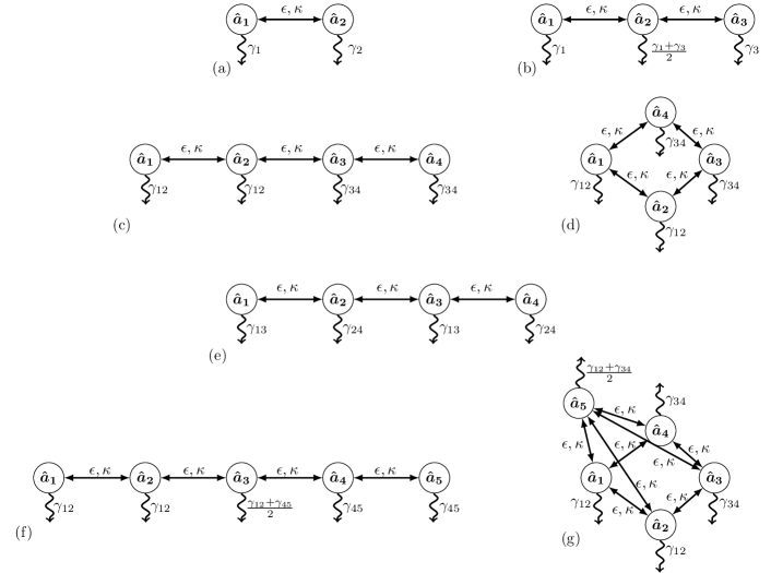
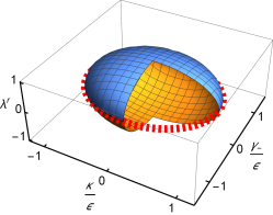
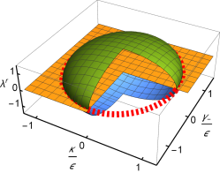
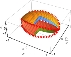
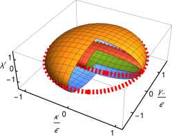
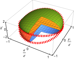
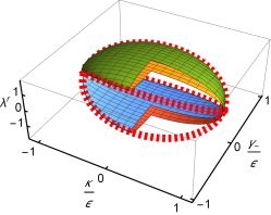
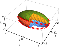
Figure 2: Real parts λr\lambda^{\rm r} of the eigenvalues (a) λ1,2M(2)\lambda_{1,2}^{M^{(2)}} of the matrix 𝑴(𝟐)\bm{M^{(2)}}, given in Eq. (15), for the two-mode bosonic system, (b) λ1,2,3M(3)\lambda_{1,2,3}^{M^{(3)}} of the matrix 𝑴(𝟑)\bm{M^{(3)}}, given in Eq. (35), for the three-mode linear bosonic system, (c) [(d)] λ1,,4Ml1(4)\lambda_{1,\ldots,4}^{M^{(4)}_{\rm l1}} [λ1,,4Ml2(4)\lambda_{1,\ldots,4}^{M^{(4)}_{\rm l2}}] of the matrix 𝑴𝐥𝟏(𝟒)\bm{M^{(4)}_{\rm l1}} [𝑴𝐥𝟐(𝟒)\bm{M^{(4)}_{\rm l2}}], given in Eqs. (IV.1), (45), and [(49)] for the four-mode linear bosonic system with neighbor modes having equal [different] damping and/or amplification rates, (e) λ1,,4Mc1(4)\lambda_{1,\ldots,4}^{M^{(4)}_{\rm c1}} of the matrix 𝑴𝐜𝟏(𝟒)\bm{M^{(4)}_{\rm c1}}, given in Eq. (IV.2), for the four-mode circular bosonic system with neighbor modes having equal the damping and/or amplification rates, (f) λ2,,5Ml(5)\lambda_{2,\ldots,5}^{M^{(5)}_{\rm l}} of the matrix 𝑴𝐥(𝟓)\bm{M^{(5)}_{\rm l}}, given by Eq. (V.1), for the five-mode linear bosonic system, and (g,h) λ2,,5Mp(5)\lambda_{2,\ldots,5}^{M^{(5)}_{\rm p}} of the matrix 𝑴𝐩(𝟓)\bm{M^{(5)}_{\rm p}}, given in Eq. (V.2), for the five-mode pyramid bosonic system assuming (g) β1=0\beta_{1}=0 and (h) β2=0\beta_{2}=0. The eigenvalues are drawn in the parameter space (κ/ϵ,γ/ϵ)(\kappa/\epsilon,\gamma_{-}/\epsilon), where ϵ\epsilon (κ\kappa) is the linear (nonlinear) coupling strength and γ\gamma_{-} the difference of the damping/amplification rates in individual models. Dashed red curves indicate the positions of the QHPs given by (a,e,g) Eq. (22), (b) Eq. (37), (c) Eq. (48), (d) Eq. (52), (f) Eq. (74), and (h) Eq. (86).

Deeper insight into the structure of higher-order FOMs, as well as the system dynamics, can be obtained once we transform the Heisenberg-Langevin equations (2) into the form in which the dynamical matrix has the diagonal form. Using the transformation matrix 𝑷=[𝒀𝟏𝑴(𝟐),𝒀𝟐𝑴(𝟐),𝒀𝟑𝑴(𝟐),𝒀𝟒𝑴(𝟐)]\bm{P}=\left[\bm{Y_{1}^{M^{(2)}}},\bm{Y_{2}^{M^{(2)}}},\bm{Y_{3}^{M^{(2)}}},\bm{Y_{4}^{M^{(2)}}}\right] formed from the eigenvectors in Eq. (16), we define the corresponding field operators 𝒃^=[b^1,b^2,b^1,b^2]T\hat{\bm{b}}=\left[\hat{b}_{1},\hat{b}_{2},\hat{b}_{1}^{\dagger},\hat{b}_{2}^{\dagger}\right]^{T}, the Langevin operator forces 𝑲^=[K^1,K^2,K^1,K^2]T\hat{\bm{K}}=\left[\hat{K}_{1},\hat{K}_{2},\hat{K}_{1}^{\dagger},\hat{K}_{2}^{\dagger}\right]^{T}, and the diagonal dynamical matrix 𝚲(𝟐)\bm{\Lambda^{(2)}}:

𝚲(𝟐)=𝑷1𝑴(𝟐)𝑷,𝒃^=𝑷1𝒂^,𝑲^=𝑷1𝑳^.\displaystyle\bm{\Lambda^{(2)}}=\bm{P}^{-1}\bm{M^{(2)}}\bm{P},\hskip 8.53581pt\hat{\bm{b}}=\bm{P}^{-1}\hat{\bm{a}},\hskip 8.53581pt\hat{\bm{K}}=\bm{P}^{-1}\hat{\bm{L}}. (23)

We note that the order of elements in the operator vector 𝒃^\hat{\bm{b}} (and similarly in the vector 𝑲^\hat{\bm{K}} of the accompanying Langevin operator forces) is given by the numbering of the eigenvalues in Eq. (15) and the corresponding diagonalization transform.

In the transformed basis, the Heisenberg-Langevin equations take the form:

d𝒃^dt\displaystyle\frac{d\hat{\bm{b}}}{dt} =\displaystyle= i𝚲(𝟐)𝒃^+𝑲^.\displaystyle-i\bm{\Lambda^{(2)}}\hat{\bm{b}}+\hat{\bm{K}}. (24)

We note that the positions of the newly-defined annihilation and creation operators in the vector 𝒃^\hat{\bm{b}}, as well as the positions of the accompanying Langevin operator forces in the vector 𝑲^\hat{\bm{K}}, differ from those in the original vectors 𝒂^\hat{\bm{a}} and 𝑳^\hat{\bm{L}} defined above Eq. (2). The solution to Eq. (24) is expressed as:

𝒃^(t)\displaystyle\hat{\bm{b}}(t) =\displaystyle= exp(i𝚲(𝟐)t)𝒃^(0)\displaystyle\exp(-i\bm{\Lambda^{(2)}}t)\hat{\bm{b}}(0) (25)
+0tdtexp[i𝚲(𝟐)(tt)]𝑲^(t).\displaystyle\mbox{}+\int_{0}^{t}dt^{\prime}\exp[-i\bm{\Lambda^{(2)}}(t-t^{\prime})]\hat{\bm{K}}(t^{\prime}).

Using the inverse transformation, we arrive at the solution for the operators 𝒂^\hat{\bm{a}}, which reads:

𝒂^(t)\displaystyle\hat{\bm{a}}(t) =\displaystyle= 𝑷exp(i𝚲(𝟐)t)𝑷1𝒂^(0)\displaystyle\bm{P}\exp(-i\bm{\Lambda^{(2)}}t)\bm{P}^{-1}\hat{\bm{a}}(0) (26)
+0tdt𝑷exp[i𝚲(𝟐)(tt)]𝑷1𝑳^(t).\displaystyle\mbox{}+\int_{0}^{t}dt^{\prime}\bm{P}\exp[-i\bm{\Lambda^{(2)}}(t-t^{\prime})]\bm{P}^{-1}\hat{\bm{L}}(t^{\prime}).

The solution in Eq. (26) of the Heisenberg-Langevin equations in the diagonal form together with the assumption of the Gaussian Markovian character of the Langevin operator forces allows us to follow the dynamics of FOMs of an arbitrary order. We note that, from the point of view of eigenfrequencies, the FOMs of a given order form a closed dynamical system Peřina Jr. et al. 2022. In this dynamics, we observe the genuine QEPs and QHPs that are derived from the inherited QEPs and QHPs discussed above. In general, the higher is the FOM order, the higher are the observed EDs and DDs at QEPs and QHPs. These degeneracies were systematically studied in Ref. Peřina Jr. et al. 2022 up to the fourth-order FOMs. Here, we summarize in Tab. 1 these degeneracies for up to second-order FOMs to give the comparison of the QEP and QHP degeneracies found in the first- and second-order FOM dynamics. It is useful to compare QEP and QHP degeneracies in Tab. 1 with those observed in the systems with greater numbers of modes presented below.

𝚲𝒋𝐢\bm{\Lambda^{\rm i}_{j}} 𝚲𝒋𝐫\bm{\Lambda^{\rm r}_{j}} Moments Moment Genuine and induced QHPs Genuine QHPs
deg. Partial Partial Partial Partial
QDP x QDP x QDP x QDP x
QEP deg. QEP deg. QEP deg. QEP deg.
γ+\gamma_{+} β\mp\beta b^1\langle\hat{b}_{1}\rangle, b^1\langle\hat{b}_{1}^{\dagger}\rangle 𝑩^𝟏\langle\bm{\hat{B}_{1}}\rangle 1 1x2 2x2 1x2 2x2
b^2\langle\hat{b}_{2}\rangle, b^2\langle\hat{b}_{2}^{\dagger}\rangle 𝑩^𝟐\langle\bm{\hat{B}_{2}}\rangle 1 1x2 1x2
2γ+2\gamma_{+} 2β\mp 2\beta b^1b^2\langle\hat{b}_{1}\hat{b}_{2}\rangle, b^1b^2\langle\hat{b}_{1}^{\dagger}\hat{b}_{2}^{\dagger}\rangle 𝑩^𝟏𝑩^𝟐\langle\bm{\hat{B}_{1}\hat{B}_{2}}\rangle 2 2x4 4x4 1x4 1x4
ββ\beta-\beta b^1b^2\langle\hat{b}_{1}^{\dagger}\hat{b}_{2}\rangle 2 +
ββ\beta-\beta b^1b^2\langle\hat{b}_{1}\hat{b}_{2}^{\dagger}\rangle 2
2β\mp 2\beta b^12\langle\hat{b}_{1}^{2}\rangle, b^12\langle\hat{b}_{1}^{\dagger 2}\rangle 𝑩^𝟏𝟐\langle\bm{\hat{B}_{1}^{2}}\rangle 1 1x4 1x3 2x3
ββ\beta-\beta b^1b^1\langle\hat{b}_{1}^{\dagger}\hat{b}_{1}\rangle 2
2β\mp 2\beta b^22\langle\hat{b}_{2}^{2}\rangle, b^22\langle\hat{b}_{2}^{\dagger 2}\rangle 𝑩^𝟐𝟐\langle\bm{\hat{B}_{2}^{2}}\rangle 1 1x4 1x3
ββ\beta-\beta b^2b^2\langle\hat{b}_{2}^{\dagger}\hat{b}_{2}\rangle 2
Table 1: Real and imaginary parts of the complex eigenfrequencies 𝚲𝒋𝐫i𝚲𝒋𝐢\bm{\Lambda_{j}^{\rm r}}-i\bm{\Lambda_{j}^{\rm i}} of the matrix 𝑴(𝟐)\bm{M^{(2)}} given in Eq. (II) for the two-mode bosonic system derived from the equations for the FOMs up to second order. The corresponding moments in the ‘diagonalized’ field operators are written together with their degeneracies (deg.) coming from different positions of the field operators. The DDs of QHPs (partial DDs) derived from the indicated FOMs and the EDs of the constituting QEPs are given. Both genuine and induced QEPs and QHPs are considered. The operators 𝑩^𝒋\bm{\hat{B}_{j}} for j=1,2j=1,2 are defined in the lines written for 𝚲𝒋𝐢=γ+\bm{\Lambda^{\rm i}_{j}}=\gamma_{+} devoted to the first-order FOMs.

We note that the quadratic form of Hamiltonian H^2\hat{H}_{2}, in Eq. (1), is not the most general one. It can be extended by considering additional terms describing local squeezing in modes 1 and 2 described by a constant gg, as it was done in Ref. Peřina Jr. et al. 2022:

H~^2=[ϵa^1a^2+κa^1a^2+j=1,2ga^j2/2]+H.c.\displaystyle\hat{\tilde{H}}_{2}=\left[\hbar\epsilon\hat{a}^{\dagger}_{1}\hat{a}_{2}+\hbar\kappa\hat{a}_{1}\hat{a}_{2}+\sum_{j=1,2}\hbar g\hat{a}_{j}^{\dagger 2}/2\right]+{\rm H.c.} (27)

However, the structure of the dynamical matrix 𝑴(𝟐)\bm{M^{(2)}}, built from the 2×22\times 2 submatrices, is broken for nonzero values of the constant gg. This results in the loss of the second-order DD that follows from the structure of the 𝝃\bm{\xi} and 𝜸~𝒋\bm{\tilde{\gamma}_{j}} matrices written in Eq. (II). As a consequence, only second-order inherited QEPs occur for g0g\neq 0 in the parameter space (κ/ϵ,γ/ϵ,g/ϵ)(\kappa/\epsilon,\gamma_{-}/\epsilon,g/\epsilon). Detailed analysis of the positions of inherited QEPs, as well as EDs and DDs of QEPs and QHPs observed in the FOMs dynamics was provided in Ref. Peřina Jr. et al. 2022. Similar reduction of eigenvalue and eigenvector degeneracies in the Hilbert space after including these terms was observed in more complex bosonic systems. We further pay attention only to the systems described by quadratic Hamiltonians without these terms.

III Three-mode bosonic system

The above-analyzed two-mode system provided QHPs with second-order ED and DD. Whereas the DD originates in the mutual coupling between the two modes (described by the strengths ϵ\epsilon and κ\kappa), the ED arises from different strengths of damping and amplification of the modes and a given system configuration. Bosonic systems composed of more than two modes give a promise for revealing QHPs with a larger number of EDs and DDs. However, the question is how to choose a suitable configuration of interactions among the modes and their damping and/or amplification rates. Whereas the parity symmetry is useful in seeking promising geometries, the temporal symmetry allows to define suitable relations among the damping and amplification rates. In this section, we begin our investigation by considering three-mode bosonic systems in the linear configuration, and define specific conditions under which QHPs occur. In the following sections, we extend our analysis to the four- and five-mode systems. The geometries together with their characteristic parameters are schematically shown in Fig. 1. We also identify the positions of QHPs in the corresponding parameter spaces. Moreover, we analyze the occurrence of genuine QEPs and QHPs and determine their EDs and DDs from the point of view of the dynamics of second-order FOMs.

Among the bosonic systems with three modes we succeeded in identifying QHPs in the linear configuration that is shown in Fig. 1(b). Similar system in this configuration was experimentally realized in Ref. Hodaei et al. 2017. We note that a QEP with third-order ED was identified in Ref. Jing et al. 2017 in an optomechanical system of three interacting bosonic modes. Hamiltonian H^3\hat{H}_{3} of such a system can be written as follows:

H^3\displaystyle\hat{H}_{3} =\displaystyle= [ϵa^1a^2+ϵa^2a^3+κa^1a^2+κa^2a^3]+H.c.\displaystyle\left[\hbar\epsilon\hat{a}_{1}^{\dagger}\hat{a}_{2}+\hbar\epsilon\hat{a}_{2}^{\dagger}\hat{a}_{3}+\hbar\kappa\hat{a}_{1}\hat{a}_{2}+\hbar\kappa\hat{a}_{2}\hat{a}_{3}\right]+\textrm{H.c.}

Using the 2×22\times 2 submatrices 𝜸~𝒋\bm{\tilde{\gamma}_{j}}, j=1,2,3j=1,2,3, describing mode damping or amplification, and 𝝃\bm{\xi} defined in Eq. (II), we derive the Heisenberg-Langevin equations in the form

d𝒂^dt\displaystyle\frac{d\hat{\bm{a}}}{dt} =\displaystyle= i𝑴(𝟑)𝒂^+𝑳^,\displaystyle-i\bm{M^{(3)}}\hat{\bm{a}}+\hat{\bm{L}}, (29)

where

𝑴(𝟑)\displaystyle\bm{M^{(3)}} =\displaystyle= [i𝜸~𝟏𝝃𝟎𝝃i𝜸~𝟐𝝃𝟎𝝃i𝜸~𝟑],\displaystyle\left[\begin{array}[]{ccc}-i\bm{\tilde{\gamma}_{1}}&\bm{\xi}&\bm{0}\\ \bm{\xi}&-i\bm{\tilde{\gamma}_{2}}&\bm{\xi}\\ \bm{0}&\bm{\xi}&-i\bm{\tilde{\gamma}_{3}}\\ \end{array}\right],

and 𝟎\bm{0} denotes the 2×22\times 2 null matrix, while 𝒂^=[𝒂^𝟏,𝒂^𝟐,𝒂^𝟑]T[a^1,a^1,a^2,a^2,a^3,a^3]T\hat{\bm{a}}=\left[\hat{\bm{a}}_{\bm{1}},\hat{\bm{a}}_{\bm{2}},\hat{\bm{a}}_{\bm{3}}\right]^{T}\equiv\left[\hat{a}_{1},\hat{a}_{1}^{\dagger},\hat{a}_{2},\hat{a}_{2}^{\dagger},\hat{a}_{3},\hat{a}_{3}^{\dagger}\right]^{T} and 𝑳^=[L^1,L^1,L^2,L^2,L^3,L^3]T\hat{\bm{L}}=\left[\hat{L}_{1},\hat{L}_{1}^{\dagger},\hat{L}_{2},\hat{L}_{2}^{\dagger},\hat{L}_{3},\hat{L}_{3}^{\dagger}\right]^{T}.

Assuming the condition

2γ2=γ1+γ3,2\gamma_{2}=\gamma_{1}+\gamma_{3}, (34)

the eigenvalues λjM(3)\lambda_{j}^{M^{(3)}} (j=1,2,3j=1,2,3) of the dynamical matrix 𝑴(𝟑)\bm{M^{(3)}} in Eq. (III) share the common damping or amplification rate γ+\gamma_{+} and we may write

λ1M(3)\displaystyle\lambda_{1}^{M^{(3)}} =\displaystyle= iγ+,λ2,3M(3)=iγ+β,\displaystyle-i\gamma_{+},\quad\lambda_{2,3}^{M^{(3)}}=-i\gamma_{+}\mp\beta, (35)

using 4γ±=γ1±γ34\gamma_{\pm}=\gamma_{1}\pm\gamma_{3} and β2=2ξ2γ2\beta^{2}=2\xi^{2}-\gamma_{-}^{2}; ξ\xi being an eigenvalue of the matrix 𝝃\bm{\xi} in Eq. (II). The eigenvectors corresponding to the eigenvalues λjM(3)\lambda_{j}^{M^{(3)}} in Eq. (35) are derived in the form:

𝒚𝟏𝑴(𝟑)\displaystyle\bm{y_{1}^{M^{(3)}}} =\displaystyle= [1,iγξ,1]T,\displaystyle\left[-1,-\frac{i\gamma_{-}}{\xi},1\right]^{T},
𝒚𝟐,𝟑𝑴(𝟑)\displaystyle\bm{y_{2,3}^{M^{(3)}}} =\displaystyle= [1+iγ(iγ±β)ξ2,iγ±βξ,1]T.\displaystyle\left[1+\frac{i\gamma_{-}(i\gamma_{-}\pm\beta)}{\xi^{2}},-\frac{i\gamma_{-}\pm\beta}{\xi},1\right]^{T}. (36)

Provided that β=0\beta=0, the three eigenvalues λjM(3)\lambda_{j}^{M^{(3)}} for j=1,2,3j=1,2,3 in Eq. (35), as well as the corresponding eigenvectors in Eq. (36), are equal and, thus, third-order QEPs of the 3×33\times 3 matrix 𝑴(𝟑)\bm{M^{(3)}} are found. Taking into account the structure of the submatrices of the matrix 𝑴(𝟑)\bm{M^{(3)}}, these QEPs are in fact QHPs with second-order DD. Substituting for the eigenvalues ξ\xi of matrix 𝝃\bm{\xi} from Eq. (13), the condition β=2ζ2γ2=0\beta=\sqrt{2\zeta^{2}-\gamma_{-}^{2}}=0 for having a QHP attains the form:

κ2ϵ2+γ22ϵ2=1.\frac{\kappa^{2}}{\epsilon^{2}}+\frac{\gamma_{-}^{2}}{2\epsilon^{2}}=1. (37)

This condition is visualized by the red dashed curve in Fig. 2(b) that shows the real parts of the eigenvalues λjM(3)\lambda_{j}^{M^{(3)}} as they vary in the parameter space (κ/ϵ,γ/ϵ)(\kappa/\epsilon,\gamma_{-}/\epsilon).

The analysis of QEPs and QHPs appropriate for the FOM dynamics requires the construction of eigenvalues and eigenvectors of the matrix 𝑴(𝟑)\bm{M^{(3)}} in its full 6×66\times 6 space combining the eigenvalues and eigenvectors in Eqs. (36) and (37) with those of the matrix 𝝃\bm{\xi} given in Eqs. (13) and (14). They are written in Appendix A. The obtained eigenvectors then allow us to introduce new field operators 𝒃^=[b^1,b^1,b^2,b^3,b^2,b^3]T\hat{\bm{b}}=\left[\hat{b}_{1},\hat{b}_{1}^{\dagger},\hat{b}_{2},\hat{b}_{3},\hat{b}_{2}^{\dagger},\hat{b}_{3}^{\dagger}\right]^{T} in which the dynamical matrix 𝑴(𝟑)\bm{M^{(3)}} of the Heisenberg-Langevin equations attains its diagonal form 𝚲(𝟑)\bm{\Lambda^{(3)}}, similarly as it was done in Sec. II in the case of the two-mode system. The QEPs and QHPs predicted in the dynamics of the first- and second-order FOMs are summarized in Tab. 2.

𝚲𝒋𝐢\bm{\Lambda^{\rm i}_{j}} 𝚲𝒋𝐫\bm{\Lambda^{\rm r}_{j}} Moments Moment Genuine and induced QHPs Genuine QHPs
deg. Partial Partial Partial Partial
QDP x QDP x QDP x QDP x
QEP deg. QEP deg. QEP deg. QEP deg.
γ+\gamma_{+} 0, β\mp\beta b1\langle b_{1}\rangle, b2\langle b_{2}\rangle, b2\langle b_{2}^{\dagger}\rangle 𝑩^𝟏\langle\bm{\hat{B}_{1}}\rangle 1 1x3 2x3 1x3 2x3
0, β\mp\beta b1\langle b_{1}^{\dagger}\rangle, b3\langle b_{3}\rangle, b3\langle b_{3}^{\dagger}\rangle 𝑩^𝟐\langle\bm{\hat{B}_{2}}\rangle 1 1x3 1x3
2γ+2\gamma_{+} 00 b12\langle b_{1}^{2}\rangle 𝑩^𝟏𝟐\langle\bm{\hat{B}_{1}^{2}}\rangle 1 1x9 4x9 1x6 2x6
β\mp\beta b1b2\langle b_{1}b_{2}\rangle, b1b2\langle b_{1}b_{2}^{\dagger}\rangle 2 +
2β\mp 2\beta b22\langle b_{2}^{2}\rangle, b22\langle b_{2}^{\dagger 2}\rangle 1
ββ\beta-\beta b2b2\langle b_{2}^{\dagger}b_{2}\rangle 2
0 b1b1\langle b_{1}^{\dagger}b_{1}\rangle 𝑩^𝟐𝑩^𝟏\langle\bm{\hat{B}_{2}\hat{B}_{1}}\rangle 2 2x9 1x9 1x9
β\mp\beta b1b2\langle b_{1}^{\dagger}b_{2}\rangle, b1b2\langle b_{1}^{\dagger}b_{2}^{\dagger}\rangle 2
β\mp\beta b3b1\langle b_{3}b_{1}\rangle, b3b1\langle b_{3}^{\dagger}b_{1}\rangle 2
2β\mp 2\beta b3b2\langle b_{3}b_{2}\rangle, b3b2\langle b_{3}^{\dagger}b_{2}^{\dagger}\rangle 2
ββ\beta-\beta b3b2\langle b_{3}b_{2}^{\dagger}\rangle, b3b2\langle b_{3}^{\dagger}b_{2}\rangle 2
00 b12\langle b_{1}^{\dagger 2}\rangle 𝑩^𝟐𝟐\langle\bm{\hat{B}_{2}^{2}}\rangle 1 1x9 1x6
β\mp\beta b1b3\langle b_{1}^{\dagger}b_{3}\rangle, b1b3\langle b_{1}^{\dagger}b_{3}^{\dagger}\rangle 2
2β\mp 2\beta b32\langle b_{3}^{2}\rangle, b33\langle b_{3}^{\dagger 3}\rangle 1
ββ\beta-\beta b3b3\langle b_{3}^{\dagger}b_{3}\rangle 2
Table 2: Real and imaginary parts of the complex eigenfrequencies 𝚲𝒋𝐫i𝚲𝒋𝐢\bm{\Lambda_{j}^{\rm r}}-i\bm{\Lambda_{j}^{\rm i}} of the matrix 𝑴(𝟑)\bm{M^{(3)}}, given in Eq. (III), for the linear three-mode bosonic system derived from the equations for the FOMs up to second order. For details, see the caption to Tab. 1.

IV Four-mode bosonic systems

Let us move to the investigations of four-mode bosonic systems, in which we revealed QEPs and QHPs in two arrangements: linear and circular. In the linear arrangement, we consider two configurations that differ by the damping and/or amplification rates assigned to the modes: Either the neighbor modes share their damping and/or amplification rates or their rates differ. On the other hand, equal damping and/or amplification rates of the neighbor modes are needed in the circular arrangement to reveal QEPs and QHPs.

IV.1 Linear configurations

In the linear configuration, the quadratic Hamiltonian H^4,l\hat{H}_{4,{\rm l}} of four-mode system is expressed in the form

H^4,l\displaystyle\hat{H}_{4,{\rm l}} =\displaystyle= [ϵa^1a^2+ϵa^2a^3+ϵa^3a^4+κa^1a^2\displaystyle\Bigl[\hbar\epsilon\hat{a}_{1}^{\dagger}\hat{a}_{2}+\hbar\epsilon\hat{a}_{2}^{\dagger}\hat{a}_{3}+\hbar\epsilon\hat{a}_{3}^{\dagger}\hat{a}_{4}+\hbar\kappa\hat{a}_{1}\hat{a}_{2} (38)
+κa^2a^3+κa^3a^4]+H.c.\displaystyle+\hbar\kappa\hat{a}_{2}\hat{a}_{3}+\hbar\kappa\hat{a}_{3}\hat{a}_{4}\Bigr]+\textrm{H.c.}

The corresponding Heisenberg-Langevin equations are derived as follows:

d𝒂^dt\displaystyle\frac{d\hat{\bm{a}}}{dt} =\displaystyle= i𝑴𝐥(𝟒)𝒂^+𝑳^,\displaystyle-i\bm{M^{(4)}_{\rm l}}\hat{\bm{a}}+\hat{\bm{L}}, (39)

Using the 2×22\times 2 submatrices defined in Eq. (II) we write the dynamical matrix 𝑴𝐥(𝟒)\bm{M^{(4)}_{\rm l}}:

𝑴𝐥(𝟒)\displaystyle\bm{M^{(4)}_{\rm l}} =\displaystyle= [i𝜸~𝟏𝝃𝟎𝟎𝝃i𝜸~𝟐𝝃𝟎𝟎𝝃i𝜸~𝟑𝝃𝟎𝟎𝝃i𝜸~𝟒].\displaystyle\left[\begin{array}[]{cccc}-i\bm{\tilde{\gamma}_{1}}&\bm{\xi}&\bm{0}&\bm{0}\\ \bm{\xi}&-i\bm{\tilde{\gamma}_{2}}&\bm{\xi}&\bm{0}\\ \bm{0}&\bm{\xi}&-i\bm{\tilde{\gamma}_{3}}&\bm{\xi}\\ \bm{0}&\bm{0}&\bm{\xi}&-i\bm{\tilde{\gamma}_{4}}\\ \end{array}\right].

The vectors 𝒂^\hat{\bm{a}} of field operators and 𝑳^\hat{\bm{L}} of the Langevin operator forces in Eq. (39) are given as 𝒂^=[𝒂^𝟏,𝒂^𝟐,𝒂^𝟑,𝒂^𝟒]T[a^1,a^1,a^2,a^2,a^3,a^3,a^4,a^4]T\hat{\bm{a}}=\left[\hat{\bm{a}}_{\bm{1}},\hat{\bm{a}}_{\bm{2}},\hat{\bm{a}}_{\bm{3}},\hat{\bm{a}}_{\bm{4}}\right]^{T}\equiv\left[\hat{a}_{1},\hat{a}_{1}^{\dagger},\hat{a}_{2},\hat{a}_{2}^{\dagger},\hat{a}_{3},\hat{a}_{3}^{\dagger},\hat{a}_{4},\hat{a}_{4}^{\dagger}\right]^{T} and 𝑳^=[L^1,L^1,L^2,L^2,L^3,L^3,L^4,L^4]T\hat{\bm{L}}=\left[\hat{L}_{1},\hat{L}_{1}^{\dagger},\hat{L}_{2},\hat{L}_{2}^{\dagger},\hat{L}_{3},\hat{L}_{3}^{\dagger},\hat{L}_{4},\hat{L}_{4}^{\dagger}\right]^{T}.

QEPs and QHPs have been found in the following two configurations:

IV.1.1 Linear configuration with equal damping and/or amplification rates of neighbor modes

In this configuration schematically shown in Fig. 2(c) we assume equal damping and/or amplification rates in modes 1 and 2, and also modes 3 and 4:

γ1=γ2γ12,γ3=γ4γ34.\gamma_{1}=\gamma_{2}\equiv\gamma_{12},\hskip 14.22636pt\gamma_{3}=\gamma_{4}\equiv\gamma_{34}. (45)

In this case, diagonalization of the dynamical matrix 𝑴𝐥𝟏(𝟒)\bm{M^{(4)}_{\rm l1}} in Eq. (IV.1) provides the eigenvalues

λ1,2Ml1(4)\displaystyle\lambda_{1,2}^{M^{(4)}_{\rm l1}} =\displaystyle= iγ+±α,\displaystyle-i\gamma_{+}\pm{\alpha}_{-},
λ3,4Ml1(4)\displaystyle\lambda_{3,4}^{M^{(4)}_{\rm l1}} =\displaystyle= iγ+±α+,\displaystyle-i\gamma_{+}\pm{\alpha}_{+}, (46)

and the corresponding eigenvectors

𝒚𝟏,𝟑𝑴𝐥𝟏(𝟒)\displaystyle\bm{y_{1,3}^{M^{(4)}_{\rm l1}}} =\displaystyle= [δ±2ξ3,χ2ξ21,χξ,1]T,\displaystyle\left[-\frac{\delta^{*}_{\pm}}{{2\xi^{3}}},\frac{\chi_{\mp}^{*2}}{{\xi^{2}}}-1,\frac{\chi_{\mp}^{*}}{{\xi}},1\right]^{T},
𝒚𝟐,𝟒𝑴𝐥𝟏(𝟒)\displaystyle\bm{y_{2,4}^{M^{(4)}_{\rm l1}}} =\displaystyle= [δ±2ξ3,χ2ξ21,χξ,1]T.\displaystyle\left[\frac{\delta_{\pm}}{{2\xi^{3}}},\frac{\chi_{\mp}^{2}}{{\xi^{2}}}-1,-\frac{\chi_{\mp}}{{\xi}},1\right]^{T}.

where δ±=ξ2(2iγ+χ)±2μχ\delta_{\pm}=\xi^{2}(-2i\gamma_{-}+\chi_{\mp})\pm 2\mu\chi_{\mp}, χ±=iγ++α±\chi_{\pm}=-i\gamma_{+}+\alpha_{\pm}, α±2=β2±μ\alpha_{\pm}^{2}=\beta^{2}\pm\mu, β2=3ξ2/2γ2\beta^{2}=3\xi^{2}/2-\gamma_{-}^{2}, and μ2=4ξ2(5ξ2/16γ2)\mu^{2}=4\xi^{2}(5\xi^{2}/16-\gamma_{-}^{2}) using 4γ±=γ12±γ344\gamma_{\pm}=\gamma_{12}\pm\gamma_{34}.

If μ=0\mu=0 then α+=α{\alpha}_{+}={\alpha}_{-} and χ+=χ\chi_{+}=\chi_{-}. The eigenvalues in Eq. (46) are doubly degenerated: λ1Ml1(4)=λ3Ml1(4)\lambda_{1}^{M^{(4)}_{\rm l1}}=\lambda_{3}^{M^{(4)}_{\rm l1}} and λ2Ml1(4)=λ4Ml1(4)\lambda_{2}^{M^{(4)}_{\rm l1}}=\lambda_{4}^{M^{(4)}_{\rm l1}}. The same holds also for their eigenvectors given in Eq. () and we have two QEPs with second-order ED. Similarly as in the case of three-mode bosonic system, the inclusion of the structure of submatrices in the matrix 𝑴𝐥𝟏(𝟒)\bm{M^{(4)}_{\rm l1}} gives the second-order DD to these QEPs and we, thus, have two QHPs. They are localized at the ellipse

κ2ϵ2+16γ25ϵ2=1\frac{\kappa^{2}}{\epsilon^{2}}+\frac{16\gamma_{-}^{2}}{5\epsilon^{2}}=1 (48)

defined in the parameter space (κ/ϵ,γ/ϵ)(\kappa/\epsilon,\gamma_{-}/\epsilon). Real parts of the eigenvalues λjMl1(4)\lambda_{j}^{M^{(4)}_{\rm l1}} for j=1,,4j=1,\ldots,4 are drawn in this space in Fig. 2(c).

The eigenvalues and eigenvectors of the 8×88\times 8 matrix 𝑴𝐥𝟏(𝟒)\bm{M^{(4)}_{\rm l1}} obtained by merging those written in Eqs. (46) and () and Eqs. (13) and (14) for the matrix 𝝃\bm{\xi} (for details, see Appendix A) define the transformation into the new field operators 𝒃^=[b^1,b^2,b^1,b^2,b^3,b^4,b^3,b^4]T\hat{\bm{b}}=\left[\hat{b}_{1},\hat{b}_{2},\hat{b}_{1}^{\dagger},\hat{b}_{2}^{\dagger},\hat{b}_{3},\hat{b}_{4},\hat{b}_{3}^{\dagger},\hat{b}_{4}^{\dagger}\right]^{T} in which the Heisenberg-Langevin equations have the diagonal form. This allows to reveal QEPs and QHPs in the dynamics of the first- and second-order FOMs. They are summarized in Tab. 3.

𝚲𝒋𝐢\bm{\Lambda^{\rm i}_{j}} 𝚲𝒋𝐫\bm{\Lambda^{\rm r}_{j}} Moments Moment Genuine and induced QHPs Genuine QHPs
deg. Partial Partial Partial Partial
QDP x QDP x QDP x QDP x
QEP deg. QEP deg. QEP deg. QEP deg.
γ+\gamma_{+} α±\alpha_{\pm} b1\langle b_{1}\rangle, b3\langle b_{3}\rangle 𝑩^𝟏\langle\bm{\hat{B}_{1}}\rangle 1 2x2 4x2 2x2 4x2
b4\langle b_{4}\rangle, b2\langle b_{2}\rangle 𝑩^𝟐\langle\bm{\hat{B}_{2}}\rangle 1
α±-\alpha_{\pm} b1\langle b_{1}^{\dagger}\rangle, b3\langle b_{3}^{\dagger}\rangle 𝑩^𝟑\langle\bm{\hat{B}_{3}}\rangle 1 2x2 2x2
b4\langle b_{4}^{\dagger}\rangle, b2\langle b_{2}^{\dagger}\rangle 𝑩^𝟒\langle\bm{\hat{B}_{4}}\rangle 1
2γ+2\gamma_{+} 2α±2\alpha_{\pm} b12\langle b_{1}^{2}\rangle, b32\langle b_{3}^{2}\rangle 𝑩^𝟏𝟐\langle\bm{\hat{B}_{1}^{2}}\rangle 1 1x4 16x4 1x3 4x3
α+α+\alpha_{-}+\alpha_{+} b1b3\langle b_{1}b_{3}\rangle 2 +
2α2\alpha_{\mp} b22\langle b_{2}^{2}\rangle, b42\langle b_{4}^{2}\rangle 𝑩^𝟐𝟐\langle\bm{\hat{B}_{2}^{2}}\rangle 1 1x4 1x3
α+α+\alpha_{-}+\alpha_{+} b2b4\langle b_{2}b_{4}\rangle 2
2α±-2\alpha_{\pm} b12\langle b_{1}^{\dagger 2}\rangle, b32\langle b_{3}^{\dagger 2}\rangle 𝑩^𝟑𝟐\langle\bm{\hat{B}_{3}^{2}}\rangle 1 1x4 1x3
αα+-\alpha_{-}-\alpha_{+} b1b3\langle b_{1}^{\dagger}b_{3}^{\dagger}\rangle 2
2α-2\alpha_{\mp} b22\langle b_{2}^{\dagger 2}\rangle, b42\langle b_{4}^{\dagger 2}\rangle 𝑩^𝟒𝟐\langle\bm{\hat{B}_{4}^{2}}\rangle 1 1x4 1x3
αα+-\alpha_{-}-\alpha_{+} b2b4\langle b_{2}^{\dagger}b_{4}^{\dagger}\rangle 2
α±+α±-\alpha_{\pm}+\alpha_{\pm} b1b1\langle b_{1}^{\dagger}b_{1}\rangle, b3b3\langle b_{3}^{\dagger}b_{3}\rangle 𝑩^𝟑𝑩^𝟏\langle\bm{\hat{B}_{3}\hat{B}_{1}}\rangle 2 2x4 1x4 6x4
±αα+\pm\alpha_{-}\mp\alpha_{+} b1b3\langle b_{1}^{\dagger}b_{3}\rangle, b1b3\langle b_{1}b_{3}^{\dagger}\rangle 2
α+α-\alpha_{\mp}+\alpha_{\mp} b2b2\langle b_{2}^{\dagger}b_{2}\rangle, b4b4\langle b_{4}^{\dagger}b_{4}\rangle 𝑩^𝟒𝑩^𝟐\langle\bm{\hat{B}_{4}\hat{B}_{2}}\rangle 2 2x4 1x4
α±α+\mp\alpha_{-}\pm\alpha_{+} b2b4\langle b_{2}^{\dagger}b_{4}\rangle, b4b2\langle b_{4}^{\dagger}b_{2}\rangle 2
α++α\alpha_{+}+\alpha_{-} b1b2\langle b_{1}b_{2}\rangle, b3b4\langle b_{3}b_{4}\rangle 𝑩^𝟏𝑩^𝟐\langle\bm{\hat{B}_{1}\hat{B}_{2}}\rangle 2 2x4 1x4
2α±2\alpha_{\pm} b1b4\langle b_{1}b_{4}\rangle, b3b2\langle b_{3}b_{2}\rangle 2
αα±\alpha_{\mp}-\alpha_{\pm} b1b2\langle b_{1}^{\dagger}b_{2}\rangle, b3b4\langle b_{3}^{\dagger}b_{4}\rangle 𝑩^𝟑𝑩^𝟐\langle\bm{\hat{B}_{3}\hat{B}_{2}}\rangle 2 2x4 1x4
α±α±\alpha_{\pm}-\alpha_{\pm} b1b4\langle b_{1}^{\dagger}b_{4}\rangle, b3b2\langle b_{3}^{\dagger}b_{2}\rangle 2
α±α\alpha_{\pm}-\alpha_{\mp} b2b1\langle b_{2}^{\dagger}b_{1}\rangle, b4b3\langle b_{4}^{\dagger}b_{3}\rangle 𝑩^𝟒𝑩^𝟏\langle\bm{\hat{B}_{4}\hat{B}_{1}}\rangle 2 2x4 1x4
α±α±\alpha_{\pm}-\alpha_{\pm} b4b1\langle b_{4}^{\dagger}b_{1}\rangle, b2b3\langle b_{2}^{\dagger}b_{3}\rangle 2
α+α-\alpha_{+}-\alpha_{-} b1b2\langle b_{1}^{\dagger}b_{2}^{\dagger}\rangle, b3b4\langle b_{3}^{\dagger}b_{4}^{\dagger}\rangle 𝑩^𝟑𝑩^𝟒\langle\bm{\hat{B}_{3}\hat{B}_{4}}\rangle 2 2x4 1x4
2α±-2\alpha_{\pm} b1b4\langle b_{1}^{\dagger}b_{4}^{\dagger}\rangle, b3b2\langle b_{3}^{\dagger}b_{2}^{\dagger}\rangle 2
Table 3: Real and imaginary parts of the complex eigenfrequencies 𝚲𝒋𝐫i𝚲𝒋𝐢\bm{\Lambda_{j}^{\rm r}}-i\bm{\Lambda_{j}^{\rm i}} of the matrix 𝑴𝐥𝟏(𝟒)\bm{M^{(4)}_{\rm l1}}, given in Eq. (IV.1) with Eq. (45), for the linear four-mode bosonic system with equal damping and/or amplification rates for neighbor modes derived from the equations for the FOMs up to second order. We note that α±(ζ)=α(ζ){\alpha}_{\pm}\left(\zeta\right)={\alpha}_{\mp}\left(-\zeta\right) is used here. For details, see the caption to Tab. 1.

IV.1.2 Linear configuration with different damping and/or amplification rates for neighbor modes

We assume equal the damping and/or amplification rates in modes 1 and 3 and also in modes 2 and 4:

γ1=γ3γ13,γ2=γ4γ24.\gamma_{1}=\gamma_{3}\equiv\gamma_{13},\hskip 14.22636pt\gamma_{2}=\gamma_{4}\equiv\gamma_{24}. (49)

In this configuration, which is schematically depicted in Fig. 1(e), the eigenvalues of the 4×44\times 4 dynamical matrix 𝑴𝐥𝟐(𝟒)\bm{M^{(4)}_{\rm l2}} are obtained as follows:

λ1,2Ml2(4)\displaystyle\lambda_{1,2}^{M^{(4)}_{\rm l2}} =\displaystyle= iγ+±α+,\displaystyle-i\gamma_{+}\pm\alpha_{+},
λ3,4Ml2(4)\displaystyle\lambda_{3,4}^{M^{(4)}_{\rm l2}} =\displaystyle= iγ+±α.\displaystyle-i\gamma_{+}\pm\alpha_{-}. (50)

The corresponding eigenvectors are reached in the form:

𝒚𝟏,𝟑𝑴𝐥𝟐(𝟒)\displaystyle\bm{y_{1,3}^{M^{(4)}_{\rm l2}}} =\displaystyle= [κξ,κ±,χ±ξ,1]T,\displaystyle\left[\frac{-\kappa_{\mp}}{{\xi}},\kappa_{\pm},\frac{\chi_{\pm}^{*}}{{\xi}},1\right]^{T},
𝒚𝟐,𝟒𝑴𝐥𝟐(𝟒)\displaystyle\bm{y_{2,4}^{M^{(4)}_{\rm l2}}} =\displaystyle= [κχ±ξ,κ±,χ±ξ,1]T,\displaystyle\left[\frac{\kappa_{\mp}\chi_{\pm}}{{\xi}},\kappa_{\pm},-\frac{\chi_{\pm}}{{\xi}},1\right]^{T},

where κ±=(±5+1)/2\kappa_{\pm}=(\pm\sqrt{5}+1)/2, χ±=iγ++α±{\chi}_{\pm}=-i\gamma_{+}+\alpha_{\pm}, α±2=β~±μ\alpha_{\pm}^{2}=\tilde{\beta}\pm\mu, β~=3ξ2/2γ2\tilde{\beta}=3\xi^{2}/2-\gamma_{-}^{2}, and μ=5ξ2/2\mu=\sqrt{5}\xi^{2}/2 using 4γ±=γ13±γ244\gamma_{\pm}=\gamma_{13}\pm\gamma_{24}.

Provided that α+=0\alpha_{+}=0 [α=0\alpha_{-}=0] the eigenvalues λ1Ml2(4)\lambda_{1}^{M^{(4)}_{\rm l2}} and λ2Ml2(4)\lambda_{2}^{M^{(4)}_{\rm l2}} [λ3Ml2(4)\lambda_{3}^{M^{(4)}_{\rm l2}} and λ4Ml2(4)\lambda_{4}^{M^{(4)}_{\rm l2}}] in Eq. (50) and the eigenvectors 𝒚𝟏𝑴𝐥𝟐(𝟒)\bm{y_{1}^{M^{(4)}_{\rm l2}}} and 𝒚𝟐𝑴𝐥𝟐(𝟒)\bm{y_{2}^{M^{(4)}_{\rm l2}}} [𝒚𝟑𝑴𝐥𝟐(𝟒)\bm{y_{3}^{M^{(4)}_{\rm l2}}} and 𝒚𝟒𝑴𝐥𝟐(𝟒)\bm{y_{4}^{M^{(4)}_{\rm l2}}}] in Eq. () are equal to each other and we have a QEP with second-order ED. This means that, for the 8×88\times 8 dynamical matrix 𝑴𝐥𝟐(𝟒)\bm{M^{(4)}_{\rm l2}}, we predict a QHP with second-order ED and DD observed either for α+=0\alpha_{+}=0 or α=0\alpha_{-}=0. These conditions define two ellipses in the parameter space (κ/ϵ,γ/ϵ)(\kappa/\epsilon,\gamma_{-}/\epsilon),

κ2ϵ2+2γ2(3±5)ϵ2=1.\frac{\kappa^{2}}{\epsilon^{2}}+\frac{2\gamma_{-}^{2}}{(3\pm\sqrt{5})\epsilon^{2}}=1. (52)

They are shown in Fig. 2(d) where the real parts of the eigenvalues λjMl2(4)\lambda_{j}^{M^{(4)}_{\rm l2}} for j=1,,4j=1,\ldots,4 are plotted.

The eigenvalues and eigenvectors of the 8×88\times 8 matrix 𝑴𝐥𝟐(𝟒)\bm{M^{(4)}_{\rm l2}}, given in Appendix A, determine the transformation that leaves the Heisenberg-Langevin equations in their diagonal form. Thus, we define the new field operators 𝒃^=[b^1,b^2,b^1,b^2,b^3,b^4,b^3,b^4]T\hat{\bm{b}}=\left[\hat{b}_{1},\hat{b}_{2},\hat{b}_{1}^{\dagger},\hat{b}_{2}^{\dagger},\hat{b}_{3},\hat{b}_{4},\hat{b}_{3}^{\dagger},\hat{b}_{4}^{\dagger}\right]^{T}, whose evolution identifies the QEPs and QHPs in the first- and second-order FOM dynamics given in Tab. 4.

𝚲𝒋𝐢\bm{\Lambda^{\rm i}_{j}} 𝚲𝒋𝐫\bm{\Lambda^{\rm r}_{j}} Moments Moment Genuine and induced QHPs Genuine QHPs
deg. Partial Partial Partial Partial
QDP x QDP x QDP x QDP x
QEP deg. QEP deg. QEP deg. QEP deg.
γ+\gamma_{+} ±α+\pm\alpha_{+} b1\langle b_{1}\rangle, b1\langle b_{1}^{\dagger}\rangle 𝑩^𝟏\langle\bm{\hat{B}_{1}}\rangle 1 1x2 2x2 1x2 2x2
b2\langle b_{2}\rangle, b2\langle b_{2}^{\dagger}\rangle 𝑩^𝟐\langle\bm{\hat{B}_{2}}\rangle 1 1x2 1x2
α\alpha_{-} b3\langle b_{3}\rangle 𝑩^𝟑\langle\bm{\hat{B}_{3}}\rangle 1 2x1 2x1 2x1 2x1
b4\langle b_{4}\rangle 𝑩^𝟒\langle\bm{\hat{B}_{4}}\rangle 1
α-\alpha_{-} b3\langle b_{3}^{\dagger}\rangle 𝑩^𝟓\langle\bm{\hat{B}_{5}}\rangle 1 2x1 2x1 2x1 2x1
b4\langle b_{4}^{\dagger}\rangle 𝑩^𝟔\langle\bm{\hat{B}_{6}}\rangle 1
2γ+2\gamma_{+} ±2α+\pm 2\alpha_{+} b12\langle b_{1}^{2}\rangle, b12\langle b_{1}^{\dagger 2}\rangle 𝑩^𝟏𝟐\langle\bm{\hat{B}_{1}^{2}}\rangle 1 1x4 4x4 1x3 2x3
α+α+\alpha_{+}-\alpha_{+} b1b1\langle b_{1}^{\dagger}b_{1}\rangle 2 +
±2α+\pm 2\alpha_{+} b22\langle b_{2}^{2}\rangle, b22\langle b_{2}^{\dagger 2}\rangle 𝑩^𝟐𝟐\langle\bm{\hat{B}_{2}^{2}}\rangle 1 1x4 1x3
α+α+\alpha_{+}-\alpha_{+} b2b2\langle b_{2}^{\dagger}b_{2}\rangle 2
±α+\pm\alpha_{+} b1b2\langle b_{1}b_{2}\rangle, b1b2\langle b_{1}^{\dagger}b_{2}^{\dagger}\rangle 𝑩^𝟏𝑩^𝟐\langle\bm{\hat{B}_{1}\hat{B}_{2}}\rangle 2 2x4 1x4 1x4
α+α+\alpha_{+}-\alpha_{+} b1b2\langle b_{1}^{\dagger}b_{2}\rangle, b1b2\langle b_{1}b_{2}^{\dagger}\rangle 2
α±α+\alpha_{-}\pm\alpha_{+} b1b3\langle b_{1}b_{3}\rangle, b1b3\langle b_{1}^{\dagger}b_{3}\rangle 𝑩^𝟏𝑩^𝟑\langle\bm{\hat{B}_{1}\hat{B}_{3}}\rangle 2 2x2 16x2 2x2 16x2
b1b4\langle b_{1}b_{4}\rangle, b1b4\langle b_{1}^{\dagger}b_{4}\rangle 𝑩^𝟏𝑩^𝟒\langle\bm{\hat{B}_{1}\hat{B}_{4}}\rangle 2 2x2 2x2
α±α+\alpha_{-}\pm\alpha_{+} b2b3\langle b_{2}b_{3}\rangle, b2b3\langle b_{2}^{\dagger}b_{3}\rangle 𝑩^𝟐𝑩^𝟑\langle\bm{\hat{B}_{2}\hat{B}_{3}}\rangle 2 2x2 2x2
b2b4\langle b_{2}b_{4}\rangle, b2b4\langle b_{2}^{\dagger}b_{4}\rangle 𝑩^𝟐𝑩^𝟒\langle\bm{\hat{B}_{2}\hat{B}_{4}}\rangle 2 2x2 2x2
α±α+-\alpha_{-}\pm\alpha_{+} b1b3\langle b_{1}b_{3}^{\dagger}\rangle, b1b3\langle b_{1}^{\dagger}b_{3}^{\dagger}\rangle 𝑩^𝟏𝑩^𝟓\langle\bm{\hat{B}_{1}\hat{B}_{5}}\rangle 2 2x2 2x2
b1b4\langle b_{1}b_{4}^{\dagger}\rangle, b1b4\langle b_{1}^{\dagger}b_{4}^{\dagger}\rangle 𝑩^𝟏𝑩^𝟔\langle\bm{\hat{B}_{1}\hat{B}_{6}}\rangle 2 2x2 2x2
α±α+-\alpha_{-}\pm\alpha_{+} b2b3\langle b_{2}b_{3}^{\dagger}\rangle, b2b3\langle b_{2}^{\dagger}b_{3}^{\dagger}\rangle 𝑩^𝟐𝑩^𝟓\langle\bm{\hat{B}_{2}\hat{B}_{5}}\rangle 2 2x2 2x2
b2b4\langle b_{2}b_{4}^{\dagger}\rangle, b2b4\langle b_{2}^{\dagger}b_{4}^{\dagger}\rangle 𝑩^𝟐𝑩^𝟔\langle\bm{\hat{B}_{2}\hat{B}_{6}}\rangle 2 2x2 2x2
2α2\alpha_{-} b32\langle b_{3}^{2}\rangle, b42\langle b_{4}^{2}\rangle 𝑩^𝟑𝟐\langle\bm{\hat{B}_{3}^{2}}\rangle, 𝑩^𝟒𝟐\langle\bm{\hat{B}_{4}^{2}}\rangle 1 4x1 4x1 3x1 3x1
b3b4\langle b_{3}b_{4}\rangle 𝑩^𝟑𝑩^𝟒\langle\bm{\hat{B}_{3}\hat{B}_{4}}\rangle 2
2α-2\alpha_{-} b32\langle b_{3}^{\dagger 2}\rangle, b42\langle b_{4}^{\dagger 2}\rangle 𝑩^𝟓𝟐\langle\bm{\hat{B}_{5}^{2}}\rangle, 𝑩^𝟔𝟐\langle\bm{\hat{B}_{6}^{2}}\rangle 1 4x1 4x1 3x1 3x1
b3b4\langle b_{3}^{\dagger}b_{4}^{\dagger}\rangle 𝑩^𝟓𝑩^𝟔\langle\bm{\hat{B}_{5}\hat{B}_{6}}\rangle 2
αα\alpha_{-}-\alpha_{-} b3b3\langle b_{3}^{\dagger}b_{3}\rangle, b4b4\langle b_{4}^{\dagger}b_{4}\rangle 𝑩^𝟓𝑩^𝟑\langle\bm{\hat{B}_{5}\hat{B}_{3}}\rangle, 𝑩^𝟔𝑩^𝟒\langle\bm{\hat{B}_{6}\hat{B}_{4}}\rangle 2 8x1 8x1 4x1 4x1
b3b4\langle b_{3}^{\dagger}b_{4}\rangle, b3b4\langle b_{3}b_{4}^{\dagger}\rangle 𝑩^𝟓𝑩^𝟒\langle\bm{\hat{B}_{5}\hat{B}_{4}}\rangle, 𝑩^𝟑𝑩^𝟔\langle\bm{\hat{B}_{3}\hat{B}_{6}}\rangle 2
Table 4: Real and imaginary parts of the complex eigenfrequencies 𝚲𝒋𝐫i𝚲𝒋𝐢\bm{\Lambda_{j}^{\rm r}}-i\bm{\Lambda_{j}^{\rm i}} of the matrix 𝑴𝐥𝟐(𝟒)\bm{M^{(4)}_{\rm l2}}, given in Eq. (IV.1) with Eq. (49) for the linear four-mode bosonic system with different damping and/or amplification rates of neighbor modes, as derived from the equations for the FOMs up to second order assuming α+=0\alpha_{+}=0. For details, see the caption to Tab. 1.

IV.2 Circular configuration

In the circular configuration, the Hamiltonian H^4,c\hat{H}_{4,{\rm c}} of four-mode system is expressed as

H^4,c\displaystyle\hat{H}_{4,{\rm c}} =\displaystyle= [ϵa^1a^2+ϵa^2a^3+ϵa^3a^4+ϵa^4a^1+κa^1a^2\displaystyle\left[\hbar\epsilon\hat{a}_{1}^{\dagger}\hat{a}_{2}+\hbar\epsilon\hat{a}_{2}^{\dagger}\hat{a}_{3}+\hbar\epsilon\hat{a}_{3}^{\dagger}\hat{a}_{4}+\hbar\epsilon\hat{a}_{4}^{\dagger}\hat{a}_{1}+\hbar\kappa\hat{a}_{1}\hat{a}_{2}\right. (53)
+κa^2a^3+κa^3a^4+κa^4a^1]+H.c.\displaystyle\left.+\hbar\kappa\hat{a}_{2}\hat{a}_{3}+\hbar\kappa\hat{a}_{3}\hat{a}_{4}+\hbar\kappa\hat{a}_{4}\hat{a}_{1}\right]+\textrm{H.c.}

Whereas the Heisenberg-Langevin equations keep the form of Eq. (39), the original dynamical matrix 𝑴𝐥(𝟒)\bm{M^{(4)}_{\rm l}} of the linear configuration in Eq. (IV.1) is modified into the form

𝑴𝐜(𝟒)\displaystyle\bm{M^{(4)}_{\rm c}} =\displaystyle= [i𝜸~𝟏𝝃𝟎𝝃𝝃i𝜸~𝟐𝝃𝟎𝟎𝝃i𝜸~𝟑𝝃𝝃𝟎𝝃i𝜸~𝟒].\displaystyle\left[\begin{array}[]{cccc}-i\bm{\tilde{\gamma}_{1}}&\bm{\xi}&\bm{0}&\bm{\xi}\\ \bm{\xi}&-i\bm{\tilde{\gamma}_{2}}&\bm{\xi}&\bm{0}\\ \bm{0}&\bm{\xi}&-i\bm{\tilde{\gamma}_{3}}&\bm{\xi}\\ \bm{\xi}&\bm{0}&\bm{\xi}&-i\bm{\tilde{\gamma}_{4}}\\ \end{array}\right].

We derive the eigenvalues of the matrix 𝑴𝐜(𝟒)\bm{M^{(4)}_{\rm c}} under the condition of the equal damping and/or amplification rates of the neighbor modes valid for the configuration plotted in Fig. 1(d); i.e.,

γ1=γ2γ12,γ3=γ4γ34.\gamma_{1}=\gamma_{2}\equiv\gamma_{12},\hskip 14.22636pt\gamma_{3}=\gamma_{4}\equiv\gamma_{34}. (59)

We obtain the following eigenvalues

λ1,2Mc1(4)\displaystyle\lambda_{1,2}^{M^{(4)}_{\rm c1}} =\displaystyle= iγ+α±,\displaystyle-i\gamma_{+}-\alpha_{\pm},
λ3,4Mc1(4)\displaystyle\lambda_{3,4}^{M^{(4)}_{\rm c1}} =\displaystyle= iγ++α\displaystyle-i\gamma_{+}+\alpha_{\mp} (60)

that are accompanied by the following eigenvectors

𝒚𝟏,𝟐𝑴𝐜𝟏(𝟒)\displaystyle\bm{y_{1,2}^{M^{(4)}_{\rm c1}}} =\displaystyle= [χξ,±χξ,1,1]T,\displaystyle\left[-\frac{\chi}{\xi},\pm\frac{\chi}{\xi},\mp 1,1\right]^{T},
𝒚𝟑,𝟒𝑴𝐜𝟏(𝟒)\displaystyle\bm{y_{3,4}^{M^{(4)}_{\rm c1}}} =\displaystyle= [χξ,χξ,1,1]T.\displaystyle\left[\frac{\chi^{*}}{\xi},\mp\frac{\chi^{*}}{\xi},\mp 1,1\right]^{T}. (61)

The symbols introduced in Eqs. (60) and (61) are defined as χ=iγ++β\chi=i\gamma_{+}+\beta, α±=β±ξ\alpha_{\pm}=\beta\pm\xi, β2=ξ2γ2\beta^{2}=\xi^{2}-\gamma_{-}^{2}, and 4γ±=γ12±γ344\gamma_{\pm}=\gamma_{12}\pm\gamma_{34}.

For β=0\beta=0, we have α+=α\alpha_{+}=-\alpha_{-} and χ=χ\chi^{*}=-\chi. This leads to the relations λ1Mc1(4)=λ3Mc1(4)\lambda_{1}^{M^{(4)}_{\rm c1}}=\lambda_{3}^{M^{(4)}_{\rm c1}} and λ2Mc1(4)=λ4Mc1(4)\lambda_{2}^{M^{(4)}_{\rm c1}}=\lambda_{4}^{M^{(4)}_{\rm c1}}. Also the corresponding eigenvectors coincide: 𝒚𝟏𝑴𝐜𝟏(𝟒)=𝒚𝟑𝑴𝐜𝟏(𝟒)\bm{y_{1}^{M^{(4)}_{\rm c1}}}=\bm{y_{3}^{M^{(4)}_{\rm c1}}} and 𝒚𝟐𝑴𝐜𝟏(𝟒)=𝒚𝟒𝑴𝐜𝟏(𝟒)\bm{y_{2}^{M^{(4)}_{\rm c1}}}=\bm{y_{4}^{M^{(4)}_{\rm c1}}}. As a consequence, the two QEPs with second-order EDs occur. This means that the two QHPs with second-order EDs and DDs for the 8×88\times 8 matrix 𝑴𝐜𝟏(𝟒)\bm{M^{(4)}_{\rm c1}} are formed. These QHPs occur under the condition specified in Eq. (22) that identifies the QHPs in the analyzed two-mode bosonic system. The real values of the eigenvalues λjMc1(4)\lambda_{j}^{M^{(4)}_{\rm c1}} for j=1,,4j=1,\ldots,4 are plotted in Fig. 2(e) together with the condition for the QHPs.

Using the eigenvalues and eigenvectors of the 4×44\times 4 matrix 𝑴𝐜𝟏(𝟒)\bm{M^{(4)}_{\rm c1}} and the 2×22\times 2 matrix 𝝃\bm{\xi} given in Eqs. (60), (61), (13), and (14), we arrive at the system dynamical matrix in its diagonal form (for details, see Appendix A). This brings us the new field operators 𝒃^=[b^1,b^2,b^3,b^4,b^3,b^4,b^1,b^2]T\hat{\bm{b}}=\left[\hat{b}_{1},\hat{b}_{2},\hat{b}_{3}^{\dagger},\hat{b}_{4}^{\dagger},\hat{b}_{3},\hat{b}_{4},\hat{b}_{1}^{\dagger},\hat{b}_{2}^{\dagger}\right]^{T} suitable for revealing QEPs and QHPs found in the dynamics of FOMs. As the structure of eigenvalues and eigenvectors is the same as that characterizing the four-mode linear system with equal damping and/or amplification rates of neighbor modes, the appropriate QEPs and QHPs are given in Tab. 3.

V Five-mode bosonic systems

The largest bosonic systems in our investigations consist of five bosonic modes. Among them, QEPs and QHPs were identified in two configurations: linear and pyramid.

V.1 Linear configuration

A five-mode bosonic system in its linear configuration is depicted in Fig. 1(f). Its Hamiltonian H^5,l\hat{H}_{5,{\rm l}} is given as follows:

H^5,l\displaystyle\hat{H}_{5,{\rm l}} =\displaystyle= [ϵa^1a^2+ϵa^2a^3+ϵa^3a^4+ϵa^4a^5+κa^1a^2\displaystyle\Bigl[\hbar\epsilon\hat{a}_{1}^{\dagger}\hat{a}_{2}+\hbar\epsilon\hat{a}_{2}^{\dagger}\hat{a}_{3}+\hbar\epsilon\hat{a}_{3}^{\dagger}\hat{a}_{4}+\hbar\epsilon\hat{a}_{4}^{\dagger}\hat{a}_{5}+\hbar\kappa\hat{a}_{1}\hat{a}_{2} (62)
+κa^2a^3+κa^3a^4+κa^4a^5]+H.c.\displaystyle+\hbar\kappa\hat{a}_{2}\hat{a}_{3}+\hbar\kappa\hat{a}_{3}\hat{a}_{4}+\hbar\kappa\hat{a}_{4}\hat{a}_{5}\Bigr]+\textrm{H.c.}

Defining the vectors 𝒂^=[𝒂^𝟏,𝒂^𝟐,𝒂^𝟑,𝒂^𝟒,𝒂^𝟓]T[a^1,a^1,a^2,a^2,a^3,a^3,a^4,a^4,a^5,a^5]T\hat{\bm{a}}=\left[\hat{\bm{a}}_{\bm{1}},\hat{\bm{a}}_{\bm{2}},\hat{\bm{a}}_{\bm{3}},\hat{\bm{a}}_{\bm{4}},\hat{\bm{a}}_{\bm{5}}\right]^{T}\equiv\left[\hat{a}_{1},\hat{a}_{1}^{\dagger},\hat{a}_{2},\hat{a}_{2}^{\dagger},\hat{a}_{3},\hat{a}_{3}^{\dagger},\hat{a}_{4},\hat{a}_{4}^{\dagger},\hat{a}_{5},\hat{a}_{5}^{\dagger}\right]^{T} of field operators and 𝑳^=[L^1,L^1,L^2,L^2,L^3,L^3,L^4,L^4,L^5,L^5]T\hat{\bm{L}}=\left[\hat{L}_{1},\hat{L}_{1}^{\dagger},\hat{L}_{2},\hat{L}_{2}^{\dagger},\hat{L}_{3},\hat{L}_{3}^{\dagger},\hat{L}_{4},\hat{L}_{4}^{\dagger},\hat{L}_{5},\hat{L}_{5}^{\dagger}\right]^{T} of the Langevin operator forces, we obtain the following Heisenberg-Langevin equations:

d𝒂^dt\displaystyle\frac{d\hat{\bm{a}}}{dt} =\displaystyle= i𝑴𝐥(𝟓)𝒂^+𝑳^.\displaystyle-i\bm{M^{(5)}_{\rm l}}\hat{\bm{a}}+\hat{\bm{L}}. (63)

The dynamical matrix 𝑴𝐥(𝟓)\bm{M^{(5)}_{\rm l}} introduced in Eq. (63) is written with the help of 2×22\times 2 submatrices introduced in Eq. (II) as

𝑴𝐥(𝟓)\displaystyle\bm{M^{(5)}_{\rm l}} =\displaystyle= [i𝜸~𝟏𝝃𝟎𝟎𝟎𝝃i𝜸~𝟐𝝃𝟎𝟎𝟎𝝃i𝜸~𝟑𝝃𝟎𝟎𝟎𝝃i𝜸~𝟒𝝃𝟎𝟎𝟎𝝃i𝜸~𝟓].\displaystyle\left[\begin{array}[]{ccccc}-i\bm{\tilde{\gamma}_{1}}&\bm{\xi}&\bm{0}&\bm{0}&\bm{0}\\ \bm{\xi}&-i\bm{\tilde{\gamma}_{2}}&\bm{\xi}&\bm{0}&\bm{0}\\ \bm{0}&\bm{\xi}&-i\bm{\tilde{\gamma}_{3}}&\bm{\xi}&\bm{0}\\ \bm{0}&\bm{0}&\bm{\xi}&-i\bm{\tilde{\gamma}_{4}}&\bm{\xi}\\ \bm{0}&\bm{0}&\bm{0}&\bm{\xi}&-i\bm{\tilde{\gamma}_{5}}\\ \end{array}\right].

Motivated by 𝒫𝒯\mathcal{PT} symmetry we assume:

γ1=γ2γ12,γ4=γ5γ45.\gamma_{1}=\gamma_{2}\equiv\gamma_{12},\hskip 14.22636pt\gamma_{4}=\gamma_{5}\equiv\gamma_{45}. (70)

Moreover, inspired by the condition in Eq. (34) derived for the three-mode linear system, we additionally assume:

2γ3=γ12+γ45.2\gamma_{3}=\gamma_{12}+\gamma_{45}. (71)

Then, diagonalization of the matrix 𝑴𝐥(𝟓)\bm{M^{(5)}_{\rm l}} results in the following eigenvalues λjMl(5){\lambda_{j}^{M^{(5)}_{\rm l}}}:

λ1Ml(5)\displaystyle\lambda_{1}^{M^{(5)}_{\rm l}} =\displaystyle= iγ+,\displaystyle-i\gamma_{+},
λ2,3Ml(5)\displaystyle\lambda_{2,3}^{M^{(5)}_{\rm l}} =\displaystyle= iγ+±α,\displaystyle-i\gamma_{+}\pm\alpha_{-},
λ4,5Ml(5)\displaystyle\lambda_{4,5}^{M^{(5)}_{\rm l}} =\displaystyle= iγ+±α+.\displaystyle-i\gamma_{+}\pm\alpha_{+}. (72)

The corresponding eigenvectors are derived as follows:

𝒚𝟏𝑴𝐥(𝟓)\displaystyle\bm{y_{1}^{M^{(5)}_{\rm l}}} =\displaystyle= [1,iγξ,γ2ξ21,iγξ,1]T,\displaystyle\left[1,\frac{i\gamma_{-}}{\xi},-\frac{\gamma_{-}^{2}}{\xi^{2}}-1,-\frac{i\gamma_{-}}{\xi},1\right]^{T},
𝒚𝟐,𝟒𝑴𝐥(𝟓)\displaystyle\bm{y_{2,4}^{M^{(5)}_{\rm l}}} =\displaystyle= [1n4ξ3,mξ32βχξ2,χ2ξ21,χξ,1]T,\displaystyle\left[-1\mp\frac{n_{\mp}}{4\xi^{3}},-\frac{m_{\mp}}{\xi^{3}}\mp\frac{2\beta\chi_{\mp}}{\xi^{2}},\frac{\chi_{\mp}^{2}}{{\xi^{2}}}-1,\frac{\chi_{\mp}}{\xi},1\right]^{T},
𝒚𝟑,𝟓𝑴𝐥(𝟓)\displaystyle\bm{y_{3,5}^{M^{(5)}_{\rm l}}} =\displaystyle= [1n4ξ3,mξ3±2βχξ2,χ2ξ21,χξ,1]T,\displaystyle\left[-1\mp\frac{n_{\mp}^{*}}{4\xi^{3}},\frac{m_{\mp}^{*}}{\xi^{3}}\pm\frac{2\beta\chi_{\mp}^{*}}{\xi^{2}},\frac{\chi_{\mp}^{*2}}{{\xi^{2}}}-1,-\frac{\chi_{\mp}^{*}}{{\xi}},1\right]^{T},

where n=(2βξ)[(2βξ)24iγα]n_{\mp}=(2\beta\mp\xi)[(2\beta\mp\xi)^{2}-4i\gamma_{-}\alpha_{\mp}], m=iγ(χ2+ξ2)m_{\mp}=i\gamma_{-}(\chi_{\mp}^{2}+\xi^{2}), χ±=iγ++α±{\chi}_{\pm}=-i\gamma_{+}+\alpha_{\pm}, α±2=β2+7ξ2/4±2βξ\alpha_{\pm}^{2}=\beta^{2}+7\xi^{2}/4\pm 2\beta\xi, β2=ξ2/4γ2\beta^{2}=\xi^{2}/4-\gamma_{-}^{2}, and 4γ±=γ12±γ454\gamma_{\pm}=\gamma_{12}\pm\gamma_{45}.

If β=0\beta=0 then α+=α\alpha_{+}=\alpha_{-} and χ+=χ\chi_{+}=\chi_{-}. Under these conditions, we have λ2Ml(5)=λ4Ml(5)\lambda_{2}^{M^{(5)}_{\rm l}}=\lambda_{4}^{M^{(5)}_{\rm l}} and 𝒚𝟐𝑴𝐥(𝟓)=𝒚𝟒𝑴𝐥(𝟓)\bm{y_{2}^{M^{(5)}_{\rm l}}}=\bm{y_{4}^{M^{(5)}_{\rm l}}}. We also have λ3Ml(5)=λ5Ml(5)\lambda_{3}^{M^{(5)}_{\rm l}}=\lambda_{5}^{M^{(5)}_{\rm l}} and 𝒚𝟑𝑴𝐥(𝟓)=𝒚𝟓𝑴𝐥(𝟓)\bm{y_{3}^{M^{(5)}_{\rm l}}}=\bm{y_{5}^{M^{(5)}_{\rm l}}}. Thus, we observe two QEPs with second-order EDs that give rise to two QHPs with second-order EDs and DDs when the 10×1010\times 10 matrix 𝑴𝐥(𝟓)\bm{M^{(5)}_{\rm l}} is analyzed. In the parameter space (κ/ϵ,γ/ϵ)(\kappa/\epsilon,\gamma_{-}/\epsilon), these QHPs are localized at the positions obeying the condition

κ2ϵ2+4γ2ϵ2=1.\frac{\kappa^{2}}{\epsilon^{2}}+\frac{4\gamma_{-}^{2}}{\epsilon^{2}}=1. (74)

The real parts of the eigenvalues λjMl(5)\lambda_{j}^{M^{(5)}_{\rm l}} forming QHPs (j=2,,5j=2,\ldots,5) are plotted in Fig. 2(f).

The eigenvalues and eigenvectors of the 10×1010\times 10 matrix 𝑴𝐥(𝟓)\bm{M^{(5)}_{\rm l}} constructed from the formulas given in Eqs. (72) and () together with those in Eqs. (13) and (14) (for details, see Appendix A) allow us to describe the system dynamics via a diagonal dynamical matrix. The appropriate operators 𝒃^=[b^1,b^1,b^2,b^3,b^2,b^3,b^4,b^5,b^4,b^5]T\hat{\bm{b}}=\left[\hat{b}_{1},\hat{b}_{1}^{\dagger},\hat{b}_{2},\hat{b}_{3},\hat{b}_{2}^{\dagger},\hat{b}_{3}^{\dagger},\hat{b}_{4},\hat{b}_{5},\hat{b}_{4}^{\dagger},\hat{b}_{5}^{\dagger}\right]^{T} then reveal QEPs and QHPs found in the dynamics of the first- and second-order FOMs (see Tab. 5).

𝚲𝒋𝐢\bm{\Lambda^{\rm i}_{j}} 𝚲𝒋𝐫\bm{\Lambda^{\rm r}_{j}} Moments Moment Genuine and induced QHPs Genuine QHPs
deg. Partial Partial Partial Partial
QDP x QDP x QDP x QDP x
QEP deg. QEP deg. QEP deg. QEP deg.
γ+\gamma_{+} α\alpha_{\mp} b2\langle b_{2}\rangle, b4\langle b_{4}\rangle 𝑩^𝟏\langle\bm{\hat{B}_{1}}\rangle 1 2x2 4x2 2x2 4x2
b3\langle b_{3}\rangle, b5\langle b_{5}\rangle 𝑩^𝟐\langle\bm{\hat{B}_{2}}\rangle 1
α-\alpha_{\mp} b2\langle b_{2}^{\dagger}\rangle, b4\langle b_{4}^{\dagger}\rangle 𝑩^𝟑\langle\bm{\hat{B}_{3}}\rangle 1 2x2 2x2
b3\langle b_{3}^{\dagger}\rangle, b5\langle b_{5}^{\dagger}\rangle 𝑩^𝟒\langle\bm{\hat{B}_{4}}\rangle 1
0 b1\langle b_{1}\rangle 𝑩^𝟓\langle\bm{\hat{B}_{5}}\rangle 1 2x1 2x1 2x1 2x1
b1\langle b_{1}^{\dagger}\rangle 𝑩^𝟔\langle\bm{\hat{B}_{6}}\rangle 1
2γ+2\gamma_{+} 2α2\alpha_{\mp} b22\langle b_{2}^{2}\rangle, b42\langle b_{4}^{2}\rangle 𝑩^𝟏𝟐\langle\bm{\hat{B}_{1}^{2}}\rangle 1 1x4 16x4 1x3 4x3
α+α+\alpha_{-}+\alpha_{+} b2b4\langle b_{2}b_{4}\rangle 2 +
2α2\alpha_{\mp} b32\langle b_{3}^{2}\rangle, b52\langle b_{5}^{2}\rangle 𝑩^𝟐𝟐\langle\bm{\hat{B}_{2}^{2}}\rangle 1 1x4 1x3
α+α+\alpha_{-}+\alpha_{+} b3b5\langle b_{3}b_{5}\rangle 2
2α-2\alpha_{\mp} b22\langle b_{2}^{\dagger 2}\rangle, b42\langle b_{4}^{\dagger 2}\rangle 𝑩^𝟑𝟐\langle\bm{\hat{B}_{3}^{2}}\rangle 1 1x4 1x3
αα+-\alpha_{-}-\alpha_{+} b2b4\langle b_{2}^{\dagger}b_{4}^{\dagger}\rangle 2
2α-2\alpha_{\mp} b32\langle b_{3}^{\dagger 2}\rangle, b52\langle b_{5}^{\dagger 2}\rangle 𝑩^𝟒𝟐\langle\bm{\hat{B}_{4}^{2}}\rangle 1 1x4 1x3
αα+-\alpha_{-}-\alpha_{+} b3b5\langle b_{3}^{\dagger}b_{5}^{\dagger}\rangle 2
2α2\alpha_{\mp} b2b3\langle b_{2}b_{3}\rangle, b4b5\langle b_{4}b_{5}\rangle 𝑩^𝟏𝑩^𝟐\langle\bm{\hat{B}_{1}\hat{B}_{2}}\rangle 2 2x4 1x4
α++α\alpha_{+}+\alpha_{-} b2b5\langle b_{2}b_{5}\rangle, b4b3\langle b_{4}b_{3}\rangle 2
α+α-\alpha_{\mp}+\alpha_{\mp} b2b2\langle b_{2}^{\dagger}b_{2}\rangle, b4b4\langle b_{4}^{\dagger}b_{4}\rangle 𝑩^𝟑𝑩^𝟏\langle\bm{\hat{B}_{3}\hat{B}_{1}}\rangle 2 2x4 1x4 6x4
α+α±-\alpha_{\mp}+\alpha_{\pm} b2b4\langle b_{2}^{\dagger}b_{4}\rangle, b2b4\langle b_{2}b_{4}^{\dagger}\rangle 2
αα\alpha_{\mp}-\alpha_{\mp} b3b2\langle b_{3}^{\dagger}b_{2}\rangle, b5b4\langle b_{5}^{\dagger}b_{4}\rangle 𝑩^𝟒𝑩^𝟏\langle\bm{\hat{B}_{4}\hat{B}_{1}}\rangle 2 2x4 1x4
α±α\alpha_{\pm}-\alpha_{\mp} b5b2\langle b_{5}^{\dagger}b_{2}\rangle, b3b4\langle b_{3}^{\dagger}b_{4}\rangle 2
αα\alpha_{\mp}-\alpha_{\mp} b2b3\langle b_{2}^{\dagger}b_{3}\rangle, b4b5\langle b_{4}^{\dagger}b_{5}\rangle 𝑩^𝟑𝑩^𝟐\langle\bm{\hat{B}_{3}\hat{B}_{2}}\rangle 2 2x4 1x4
α±α\alpha_{\pm}-\alpha_{\mp} b2b5\langle b_{2}^{\dagger}b_{5}\rangle, b4b3\langle b_{4}^{\dagger}b_{3}\rangle 2
α+α-\alpha_{\mp}+\alpha_{\mp} b3b3\langle b_{3}^{\dagger}b_{3}\rangle, b5b5\langle b_{5}^{\dagger}b_{5}\rangle 𝑩^𝟒𝑩^𝟐\langle\bm{\hat{B}_{4}\hat{B}_{2}}\rangle 2 2x4 1x4
α+α±-\alpha_{\mp}+\alpha_{\pm} b3b5\langle b_{3}^{\dagger}b_{5}\rangle, b5b3\langle b_{5}^{\dagger}b_{3}\rangle 2
2α-2\alpha_{\mp} b2b3\langle b_{2}^{\dagger}b_{3}^{\dagger}\rangle, b4b5\langle b_{4}^{\dagger}b_{5}^{\dagger}\rangle 𝑩^𝟑𝑩^𝟒\langle\bm{\hat{B}_{3}\hat{B}_{4}}\rangle 2 2x4 1x4
α+α-\alpha_{+}-\alpha_{-} b2b5\langle b_{2}^{\dagger}b_{5}^{\dagger}\rangle, b4b3\langle b_{4}^{\dagger}b_{3}^{\dagger}\rangle 2
α\alpha_{\mp} b2b1\langle b_{2}b_{1}\rangle, b4b1\langle b_{4}b_{1}\rangle 𝑩^𝟏𝑩^𝟓\langle\bm{\hat{B}_{1}\hat{B}_{5}}\rangle 2 8x2 16x2 4x2 8x2
b2b1\langle b_{2}b_{1}^{\dagger}\rangle b4b1\langle b_{4}b_{1}^{\dagger}\rangle 𝑩^𝟏𝑩^𝟔\langle\bm{\hat{B}_{1}\hat{B}_{6}}\rangle 2
b3b1\langle b_{3}b_{1}\rangle, b5b1\langle b_{5}b_{1}\rangle 𝑩^𝟐𝑩^𝟓\langle\bm{\hat{B}_{2}\hat{B}_{5}}\rangle 2
b3b1\langle b_{3}b_{1}^{\dagger}\rangle b5b1\langle b_{5}b_{1}^{\dagger}\rangle 𝑩^𝟐𝑩^𝟔\langle\bm{\hat{B}_{2}\hat{B}_{6}}\rangle 2
α-\alpha_{\mp} b2b4\langle b_{2}^{\dagger}b_{4}\rangle, b4b1\langle b_{4}^{\dagger}b_{1}\rangle 𝑩^𝟑𝑩^𝟓\langle\bm{\hat{B}_{3}\hat{B}_{5}}\rangle 2 8x2 4x2
b2b1\langle b_{2}^{\dagger}b_{1}^{\dagger}\rangle b4b1\langle b_{4}^{\dagger}b_{1}^{\dagger}\rangle 𝑩^𝟑𝑩^𝟔\langle\bm{\hat{B}_{3}\hat{B}_{6}}\rangle 2
b3b1\langle b_{3}^{\dagger}b_{1}\rangle, b5b1\langle b_{5}^{\dagger}b_{1}\rangle 𝑩^𝟒𝑩^𝟓\langle\bm{\hat{B}_{4}\hat{B}_{5}}\rangle 2
b3b1\langle b_{3}^{\dagger}b_{1}^{\dagger}\rangle b5b1\langle b_{5}^{\dagger}b_{1}^{\dagger}\rangle 𝑩^𝟒𝑩^𝟔\langle\bm{\hat{B}_{4}\hat{B}_{6}}\rangle 2
0 b12\langle b_{1}^{2}\rangle, b12\langle b_{1}^{\dagger 2}\rangle 𝑩^𝟓𝟐\langle\bm{\hat{B}_{5}^{2}}\rangle, 𝑩^𝟔𝟐\langle\bm{\hat{B}_{6}^{2}}\rangle 1 4x1 4x1 3x1 3x1
b1b1\langle b_{1}^{\dagger}b_{1}\rangle 𝑩^𝟔𝑩^𝟓\langle\bm{\hat{B}_{6}\hat{B}_{5}}\rangle 2
Table 5: Real and imaginary parts of the complex eigenfrequencies 𝚲𝒋𝐫i𝚲𝒋𝐢\bm{\Lambda_{j}^{\rm r}}-i\bm{\Lambda_{j}^{\rm i}} of the matrix 𝑴𝐥(𝟓)\bm{M^{(5)}_{\rm l}}, given in Eq. (V.1), for the five-mode linear bosonic system derived from the equations for the FOMs up to second order. For details, see the caption to Tab. 1.

V.2 Pyramid configuration

Second-order QEPs and QHPs can also be identified in the pyramid configuration [the only considered non-planar configuration, see Fig. 1(g)] described by the following Hamiltonian H^5,p\hat{H}_{5,{\rm p}}:

H^5,p\displaystyle\hat{H}_{5,{\rm p}} =\displaystyle= [ϵa^1a^2+ϵa^1a^4+ϵa^1a^5+ϵa^2a^3+ϵa^2a^5\displaystyle\left[\hbar\epsilon\hat{a}_{1}^{\dagger}\hat{a}_{2}+\hbar\epsilon\hat{a}_{1}^{\dagger}\hat{a}_{4}+\hbar\epsilon\hat{a}_{1}^{\dagger}\hat{a}_{5}+\hbar\epsilon\hat{a}_{2}^{\dagger}\hat{a}_{3}+\hbar\epsilon\hat{a}_{2}^{\dagger}\hat{a}_{5}\right. (75)
+ϵa^3a^4+ϵa^3a^5+ϵa^4a^5+κa^1a^2\displaystyle+\hbar\epsilon\hat{a}_{3}^{\dagger}\hat{a}_{4}+\hbar\epsilon\hat{a}_{3}^{\dagger}\hat{a}_{5}+\hbar\epsilon\hat{a}_{4}^{\dagger}\hat{a}_{5}+\hbar\kappa\hat{a}_{1}\hat{a}_{2}
+κa^1a^4+κa^1a^5+κa^2a^3+κa^2a^5\displaystyle+\hbar\kappa\hat{a}_{1}\hat{a}_{4}+\hbar\kappa\hat{a}_{1}\hat{a}_{5}+\hbar\kappa\hat{a}_{2}\hat{a}_{3}+\hbar\kappa\hat{a}_{2}\hat{a}_{5}
+κa^3a^4+κa^3a^5+κa^4a^5+]H.c.\displaystyle\left.+\hbar\kappa\hat{a}_{3}\hat{a}_{4}+\hbar\kappa\hat{a}_{3}\hat{a}_{5}+\hbar\kappa\hat{a}_{4}\hat{a}_{5}+\right]\textrm{H.c.}

The Hamiltonian H^5,p\hat{H}_{5,{\rm p}} given in Eq. (75) leads to the Heisenberg-Langevin equations (63) in which the dynamical matrix 𝑴𝐩(𝟓)\bm{M^{(5)}_{\rm p}} attains the form using the 2×22\times 2 submatrices introduced in Eq. (II):

𝑴𝐩(𝟓)\displaystyle\bm{M^{(5)}_{\rm p}} =\displaystyle= [i𝜸~𝟏𝝃𝟎𝝃𝝃𝝃i𝜸~𝟐𝝃𝟎𝝃𝟎𝝃i𝜸~𝟑𝝃𝝃𝝃𝟎𝝃i𝜸~𝟒𝝃𝝃𝝃𝝃𝝃i𝜸~𝟓].\displaystyle\left[\begin{array}[]{ccccc}-i\bm{\tilde{\gamma}_{1}}&\bm{\xi}&\bm{0}&\bm{\xi}&\bm{\xi}\\ \bm{\xi}&-i\bm{\tilde{\gamma}_{2}}&\bm{\xi}&\bm{0}&\bm{\xi}\\ \bm{0}&\bm{\xi}&-i\bm{\tilde{\gamma}_{3}}&\bm{\xi}&\bm{\xi}\\ \bm{\xi}&\bm{0}&\bm{\xi}&-i\bm{\tilde{\gamma}_{4}}&\bm{\xi}\\ \bm{\xi}&\bm{\xi}&\bm{\xi}&\bm{\xi}&-i\bm{\tilde{\gamma}_{5}}\\ \end{array}\right].

Motivated by the 𝒫𝒯\mathcal{PT} symmetry we assume:

γ1=γ2γ12,γ3=γ4γ34.\gamma_{1}=\gamma_{2}\equiv\gamma_{12},\hskip 14.22636pt\gamma_{3}=\gamma_{4}\equiv\gamma_{34}. (82)

Moreover, inspired by the condition (34) derived for the three-mode linear bosonic system, we additionally assume:

2γ5=γ12+γ34.2\gamma_{5}=\gamma_{12}+\gamma_{34}. (83)

Under these conditions, diagonalization of the matrix 𝑴𝐩(𝟓)\bm{M^{(5)}_{\rm p}} leaves us the following five eigenvalues λjMp(5){\lambda_{j}^{M^{(5)}_{\rm p}}}:

λ1M(5)p\displaystyle\lambda_{1}^{M^{(5)_{\rm p}}} =\displaystyle= iγ+,\displaystyle-i\gamma_{+},
λ2,3Mp(5)\displaystyle\lambda_{2,3}^{M^{(5)}_{\rm p}} =\displaystyle= iγ+ξ±β1,\displaystyle-i\gamma_{+}-\xi\pm\beta_{1},
λ4,5Mp(5)\displaystyle\lambda_{4,5}^{M^{(5)}_{\rm p}} =\displaystyle= iγ++ξ±β2.\displaystyle-i\gamma_{+}+\xi\pm\beta_{2}. (84)

The corresponding eigenvectors are obtained as follows:

𝒚𝟏𝑴𝐩(𝟓)\displaystyle\bm{y_{1}^{M^{(5)}_{\rm p}}} =\displaystyle= [iξγ,iξγ,iξγ,iξγ,1]T,\displaystyle\left[\frac{-i\xi}{\gamma_{-}},\frac{-i\xi}{\gamma_{-}},\frac{i\xi}{\gamma_{-}},\frac{i\xi}{\gamma_{-}},1\right]^{T},
𝒚𝟐𝑴𝐩(𝟓)\displaystyle\bm{y_{2}^{M^{(5)}_{\rm p}}} =\displaystyle= [χ1ξ,χ1ξ,1,1,0]T,\displaystyle\left[\frac{\chi_{1}}{\xi},-\frac{\chi_{1}}{\xi},-1,1,0\right]^{T},
𝒚𝟑𝑴𝐩(𝟓)\displaystyle\bm{y_{3}^{M^{(5)}_{\rm p}}} =\displaystyle= [χ1ξ,χ1ξ,1,1,0]T,\displaystyle\left[-\frac{\chi_{1}^{*}}{\xi},\frac{\chi_{1}^{*}}{\xi},-1,1,0\right]^{T},
𝒚𝟒𝑴𝐩(𝟓)\displaystyle\bm{y_{4}^{M^{(5)}_{\rm p}}} =\displaystyle= [σ+,σ+,σ+8,σ+,1]T,\displaystyle\left[\sigma_{+},\sigma_{+},\sigma_{+}^{8},\sigma_{+}^{*},1\right]^{T},
𝒚𝟓𝑴𝐩(𝟓)\displaystyle\bm{y_{5}^{M^{(5)}_{\rm p}}} =\displaystyle= [σ,σ,σ,σ,1]T,\displaystyle\left[\sigma_{-}^{*},\sigma_{-}^{*},\sigma_{-},\sigma_{-},1\right]^{T},

where σ±=(ξ±χ2)/(4ξ)\sigma_{\pm}=(\xi\pm\chi_{2})/(4\xi), β12=ξ2γ2\beta_{1}^{2}=\xi^{2}-\gamma_{-}^{2}, β22=5ξ2γ2\beta_{2}^{2}=5\xi^{2}-\gamma_{-}^{2}, χ1,2=β1,2iγ\chi_{1,2}=\beta_{1,2}-i\gamma_{-}, and 4γ±=γ12±γ344\gamma_{\pm}=\gamma_{12}\pm\gamma_{34}.

Contrary to the eigenvalues of the models discussed above, the eigenvalues λjMp(5)\lambda_{j}^{M^{(5)}_{\rm p}} for j=2,,5j=2,\ldots,5 in Eq. () exhibit the linear dependence on ξ\xi. This means that the DD inherited to all the above-discussed models is removed in this model. It remains only for the eigenvalue λ1Mp(5)\lambda_{1}^{M^{(5)}_{\rm p}} that, however, has no ability to form EDs.

Provided that β1=0\beta_{1}=0, we have λ2Mp(5)=λ3Mp(5)\lambda_{2}^{M^{(5)}_{\rm p}}=\lambda_{3}^{M^{(5)}_{\rm p}} and 𝒚𝟐𝑴𝐩(𝟓)=𝒚𝟑𝑴𝐩(𝟓)\bm{y_{2}^{M^{(5)}_{\rm p}}}=\bm{y_{3}^{M^{(5)}_{\rm p}}}. Thus, we have the QEP with second-order ED. When the 10×1010\times 10 matrix 𝑴𝐩(𝟓)\bm{M^{(5)}_{\rm p}} is analyzed, there occur one second-order QEP for ξ=ζ\xi=\zeta and one second-order QEP for ξ=ζ\xi=-\zeta. These QEPs occur in the parameter space (κ/ϵ,γ/ϵ)(\kappa/\epsilon,\gamma_{-}/\epsilon) under the condition written in Eq. (22).

Moreover, in parallel, if β2=0\beta_{2}=0, it holds that λ4Mp(5)=λ5Mp(5)\lambda_{4}^{M^{(5)}_{\rm p}}=\lambda_{5}^{M^{(5)}_{\rm p}} and 𝒚𝟒𝑴𝐩(𝟓)=𝒚𝟓𝑴𝐩(𝟓)\bm{y_{4}^{M^{(5)}_{\rm p}}}=\bm{y_{5}^{M^{(5)}_{\rm p}}}. Thus, similarly as above, we observe the QEP with second-order ED for the 5×55\times 5 matrix 𝑴𝐩(𝟓)\bm{M^{(5)}_{\rm p}}. There occur one second-order QEP for ξ=ζ\xi=\zeta and one second-order QEP for ξ=ζ\xi=-\zeta for the 10×1010\times 10 matrix 𝑴𝐩(𝟓)\bm{M^{(5)}_{\rm p}}. These QEPs are localized in the parameter space (κ/ϵ,γ/ϵ)(\kappa/\epsilon,\gamma_{-}/\epsilon) at the points fulfilling the condition:

κ2ϵ2+γ25ϵ2=1.\frac{\kappa^{2}}{\epsilon^{2}}+\frac{\gamma_{-}^{2}}{5\epsilon^{2}}=1. (86)

The real parts of the eigenvalues λjMp(5)\lambda_{j}^{M^{(5)}_{\rm p}} forming QEPs (j=2,,5j=2,\ldots,5) are drawn in Fig. 2(g,h).

We note that for ξ=0\xi=0 (i.e., γ=0\gamma_{-}=0, κ=ϵ\kappa=\epsilon) we have a specific QHP with ten-fold frequency degeneracy that belongs to four doubly-degenerate eigenvectors and another two eigenvectors.

The eigenvalues and eigenvectors of the 10×1010\times 10 matrix 𝑴𝐩(𝟓)\bm{M^{(5)}_{\rm p}} formed from the expressions given in Eqs. (84) and () and also in Eqs. (13) and (14) (for details, see Appendix A) allow us to analyze the system dynamics via a diagonal dynamical matrix. The appropriate operators 𝒃^=[b^1,b^1,b^2,b^3,b^3,b^2,b^4,b^5,b^5,b^4]T\hat{\bm{b}}=\left[\hat{b}_{1},\hat{b}_{1}^{\dagger},\hat{b}_{2},\hat{b}_{3},\hat{b}_{3}^{\dagger},\hat{b}_{2}^{\dagger},\hat{b}_{4},\hat{b}_{5},\hat{b}_{5}^{\dagger},\hat{b}_{4}^{\dagger}\right]^{T} then allow to identify the QEPs and QHPs observed in the dynamics of the first- and second-order FOMs, as summarized in Tab. 6).

𝚲𝒋𝐢\bm{\Lambda^{\rm i}_{j}} 𝚲𝒋𝐫\bm{\Lambda^{\rm r}_{j}} Moments Moment Genuine and induced QHPs Genuine QHPs
deg. Partial Partial Partial Partial
QDP x QDP x QDP x QDP x
QEP deg. QEP deg. QEP deg. QEP deg.
γ+\gamma_{+} ζβ2-\zeta\mp\beta_{2} b4\langle b_{4}\rangle, b5\langle b_{5}^{\dagger}\rangle 𝑩^𝟏\langle\bm{\hat{B}_{1}}\rangle 1 1x2 1x2 1x2 1x2
ζ±β2\zeta\pm\beta_{2} b4\langle b_{4}^{\dagger}\rangle, b5\langle b_{5}\rangle 𝑩^𝟐\langle\bm{\hat{B}_{2}}\rangle 1 1x2 1x2 1x2 1x2
ζβ1\zeta-\beta_{1} b2\langle b_{2}\rangle 𝑩^𝟑\langle\bm{\hat{B}_{3}}\rangle 1 1x1 1x1 1x1 1x1
ζ+β1-\zeta+\beta_{1} b2\langle b_{2}^{\dagger}\rangle 𝑩^𝟒\langle\bm{\hat{B}_{4}}\rangle 1 1x1 1x1 1x1 1x1
ζβ1-\zeta-\beta_{1} b3\langle b_{3}\rangle 𝑩^𝟓\langle\bm{\hat{B}_{5}}\rangle 1 1x1 1x1 1x1 1x1
ζ+β1\zeta+\beta_{1} b3\langle b_{3}^{\dagger}\rangle 𝑩^𝟔\langle\bm{\hat{B}_{6}}\rangle 1 1x1 1x1 1x1 1x1
0 b1\langle b_{1}\rangle 𝑩^𝟕\langle\bm{\hat{B}_{7}}\rangle 1 2x1 2x1 2x1 2x1
b1\langle b_{1}^{\dagger}\rangle 𝑩^𝟖\langle\bm{\hat{B}_{8}}\rangle 1
2γ+2\gamma_{+} 2ζ2β2-2\zeta\mp 2\beta_{2} b42\langle b_{4}^{2}\rangle, b52\langle b_{5}^{\dagger 2}\rangle 𝑩^𝟏𝟐\langle\bm{\hat{B}_{1}^{2}}\rangle 1 1x4 1x4 1x3 1x3
2ζ-2\zeta b5b4\langle b_{5}^{\dagger}b_{4}\rangle 2
2ζ±2β22\zeta\pm 2\beta_{2} b42\langle b_{4}^{\dagger 2}\rangle, b52\langle b_{5}^{2}\rangle 𝑩^𝟐𝟐\langle\bm{\hat{B}_{2}^{2}}\rangle 1 1x4 1x4 1x3 1x3
2ζ2\zeta b4b5\langle b_{4}^{\dagger}b_{5}\rangle 2
2ζ2β12\zeta-2\beta_{1} b22\langle b_{2}^{2}\rangle 𝑩^𝟑𝟐\langle\bm{\hat{B}_{3}^{2}}\rangle 1 1x1 1x1 1x1 1x1
2ζ+2β1-2\zeta+2\beta_{1} b22\langle b_{2}^{\dagger 2}\rangle 𝑩^𝟒𝟐\langle\bm{\hat{B}_{4}^{2}}\rangle 1 1x1 1x1 1x1 1x1
2ζ2β1-2\zeta-2\beta_{1} b32\langle b_{3}^{2}\rangle 𝑩^𝟓𝟐\langle\bm{\hat{B}_{5}^{2}}\rangle 1 1x1 1x1 1x1 1x1
2ζ+2β12\zeta+2\beta_{1} b32\langle b_{3}^{\dagger 2}\rangle 𝑩^𝟔𝟐\langle\bm{\hat{B}_{6}^{2}}\rangle 1 1x1 1x1 1x1 1x1
0 b12\langle b_{1}^{2}\rangle, b12\langle b_{1}^{\dagger 2}\rangle 𝑩^𝟕𝟐\langle\bm{\hat{B}_{7}^{2}}\rangle, 𝑩^𝟖𝟐\langle\bm{\hat{B}_{8}^{2}}\rangle 1 4x1 4x1 3x1 3x1
b1b1\langle b_{1}^{\dagger}b_{1}\rangle 𝑩^𝟖𝑩^𝟕\langle\bm{\hat{B}_{8}\hat{B}_{7}}\rangle 2
±2β2\pm 2\beta_{2} b4b5\langle b_{4}^{\dagger}b_{5}^{\dagger}\rangle, b4b5\langle b_{4}b_{5}\rangle 𝑩^𝟐𝑩^𝟏\langle\bm{\hat{B}_{2}\hat{B}_{1}}\rangle 2 2x4 2x4 1x4 1x4
β2β2\beta_{2}-\beta_{2} b4b4\langle b_{4}^{\dagger}b_{4}\rangle, b5b5\langle b_{5}b_{5}^{\dagger}\rangle 2
β1β2-\beta_{1}\mp\beta_{2} b4b2\langle b_{4}b_{2}\rangle, b5b2\langle b_{5}^{\dagger}b_{2}\rangle 𝑩^𝟏𝑩^𝟑\langle\bm{\hat{B}_{1}\hat{B}_{3}}\rangle 2 4x1 4x1 2x1 2x1
2ζβ1±β22\zeta-\beta_{1}\pm\beta_{2} b4b2\langle b_{4}^{\dagger}b_{2}\rangle, b5b2\langle b_{5}b_{2}\rangle 𝑩^𝟐𝑩^𝟑\langle\bm{\hat{B}_{2}\hat{B}_{3}}\rangle 2 4x1 4x1 2x1 2x1
2ζ+β1β2-2\zeta+\beta_{1}\mp\beta_{2} b2b4\langle b_{2}^{\dagger}b_{4}\rangle, b2b5\langle b_{2}^{\dagger}b_{5}^{\dagger}\rangle 𝑩^𝟒𝑩^𝟏\langle\bm{\hat{B}_{4}\hat{B}_{1}}\rangle 2 4x1 4x1 2x1 2x1
β1±β2\beta_{1}\pm\beta_{2} b2b4\langle b_{2}^{\dagger}b_{4}^{\dagger}\rangle, b2b5\langle b_{2}^{\dagger}b_{5}\rangle 𝑩^𝟒𝑩^𝟐\langle\bm{\hat{B}_{4}\hat{B}_{2}}\rangle 2 4x1 4x1 2x1 2x1
2ζβ1β2-2\zeta-\beta_{1}\mp\beta_{2} b4b3\langle b_{4}b_{3}\rangle, b5b3\langle b_{5}^{\dagger}b_{3}\rangle 𝑩^𝟏𝑩^𝟓\langle\bm{\hat{B}_{1}\hat{B}_{5}}\rangle 2 4x1 4x1 2x1 2x1
β1±β2-\beta_{1}\pm\beta_{2} b4b3\langle b_{4}^{\dagger}b_{3}\rangle, b5b3\langle b_{5}b_{3}\rangle 𝑩^𝟐𝑩^𝟓\langle\bm{\hat{B}_{2}\hat{B}_{5}}\rangle 2 4x1 4x1 2x1 2x1
β1β2\beta_{1}\mp\beta_{2} b3b4\langle b_{3}^{\dagger}b_{4}\rangle, b3b5\langle b_{3}^{\dagger}b_{5}^{\dagger}\rangle 𝑩^𝟔𝑩^𝟏\langle\bm{\hat{B}_{6}\hat{B}_{1}}\rangle 2 4x1 4x1 2x1 2x1
2ζ+β1±β22\zeta+\beta_{1}\pm\beta_{2} b3b4\langle b_{3}^{\dagger}b_{4}^{\dagger}\rangle, b3b5\langle b_{3}^{\dagger}b_{5}\rangle 𝑩^𝟔𝑩^𝟐\langle\bm{\hat{B}_{6}\hat{B}_{2}}\rangle 2 4x1 4x1 2x1 2x1
ζβ2-\zeta\mp\beta_{2} b4b1\langle b_{4}b_{1}\rangle, b5b1\langle b_{5}^{\dagger}b_{1}\rangle 𝑩^𝟕𝑩^𝟏\langle\bm{\hat{B}_{7}}\bm{\hat{B}_{1}}\rangle 2 4x2 4x2 2x2 2x2
b4b1\langle b_{4}b_{1}^{\dagger}\rangle, b5b1\langle b_{5}^{\dagger}b_{1}^{\dagger}\rangle 𝑩^𝟖𝑩^𝟏\langle\bm{\hat{B}_{8}}\bm{\hat{B}_{1}}\rangle 2
ζ±β2\zeta\pm\beta_{2} b4b1\langle b_{4}^{\dagger}b_{1}\rangle, b5b1\langle b_{5}b_{1}\rangle 𝑩^𝟕𝑩^𝟐\langle\bm{\hat{B}_{7}}\bm{\hat{B}_{2}}\rangle 2 4x2 4x2 2x2 2x2
b4b1\langle b_{4}^{\dagger}b_{1}^{\dagger}\rangle, b5b1\langle b_{5}b_{1}^{\dagger}\rangle 𝑩^𝟖𝑩^𝟐\langle\bm{\hat{B}_{8}}\bm{\hat{B}_{2}}\rangle 2
β1β1\beta_{1}-\beta_{1} b2b2\langle b_{2}^{\dagger}b_{2}\rangle 𝑩^𝟒𝑩^𝟑\langle\bm{\hat{B}_{4}\hat{B}_{3}}\rangle 2 2x1 2x1 1x1 1x1
2β1-2\beta_{1} b3b2\langle b_{3}b_{2}\rangle 𝑩^𝟓𝑩^𝟑\langle\bm{\hat{B}_{5}\hat{B}_{3}}\rangle 2 2x1 2x1 1x1 1x1
2ζ2\zeta b3b2\langle b_{3}^{\dagger}b_{2}\rangle 𝑩^𝟔𝑩^𝟑\langle\bm{\hat{B}_{6}\hat{B}_{3}}\rangle 2 2x1 2x1 1x1 1x1
ζβ1\zeta-\beta_{1} b1b2\langle b_{1}b_{2}\rangle 𝑩^𝟕𝑩^𝟑\langle\bm{\hat{B}_{7}}\bm{\hat{B}_{3}}\rangle 2 4x1 4x1 2x1 2x1
b1b2\langle b_{1}^{\dagger}b_{2}\rangle 𝑩^𝟖𝑩^𝟑\langle\bm{\hat{B}_{8}}\bm{\hat{B}_{3}}\rangle 2
2ζ-2\zeta b2b3\langle b_{2}^{\dagger}b_{3}\rangle 𝑩^𝟒𝑩^𝟓\langle\bm{\hat{B}_{4}\hat{B}_{5}}\rangle 2 2x1 2x1 1x1 1x1
2β12\beta_{1} b2b3\langle b_{2}^{\dagger}b_{3}^{\dagger}\rangle 𝑩^𝟒𝑩^𝟔\langle\bm{\hat{B}_{4}\hat{B}_{6}}\rangle 2 2x1 2x1 1x1 1x1
ζβ1-\zeta-\beta_{1} b2b1\langle b_{2}^{\dagger}b_{1}\rangle 𝑩^𝟒𝑩^𝟕\langle\bm{\hat{B}_{4}}\bm{\hat{B}_{7}}\rangle 2 4x1 4x1 2x1 2x1
b2b1\langle b_{2}^{\dagger}b_{1}^{\dagger}\rangle 𝑩^𝟒𝑩^𝟖\langle\bm{\hat{B}_{4}}\bm{\hat{B}_{8}}\rangle 2
β1β1\beta_{1}-\beta_{1} b3b3\langle b_{3}^{\dagger}b_{3}\rangle 𝑩^𝟔𝑩^𝟓\langle\bm{\hat{B}_{6}\hat{B}_{5}}\rangle 2 2x1 2x1 1x1 1x1
ζβ1-\zeta-\beta_{1} b1b3\langle b_{1}b_{3}\rangle 𝑩^𝟕𝑩^𝟓\langle\bm{\hat{B}_{7}}\bm{\hat{B}_{5}}\rangle 2 4x1 4x1 2x1 2x1
b1b3\langle b_{1}^{\dagger}b_{3}\rangle 𝑩^𝟖𝑩^𝟓\langle\bm{\hat{B}_{8}}\bm{\hat{B}_{5}}\rangle 2
ζ+β1\zeta+\beta_{1} b3b1\langle b_{3}^{\dagger}b_{1}\rangle 𝑩^𝟔𝑩^𝟕\langle\bm{\hat{B}_{6}}\bm{\hat{B}_{7}}\rangle 2 4x1 4x1 2x1 2x1
b3b1\langle b_{3}^{\dagger}b_{1}^{\dagger}\rangle 𝑩^𝟔𝑩^𝟖\langle\bm{\hat{B}_{6}}\bm{\hat{B}_{8}}\rangle 2
Table 6: Real and imaginary parts of the complex eigenfrequencies 𝚲𝒋𝐫i𝚲𝒋𝐢\bm{\Lambda_{j}^{\rm r}}-i\bm{\Lambda_{j}^{\rm i}} of the matrix 𝑴𝐩(𝟓)\bm{M^{(5)}_{\rm p}}, given in Eq. (V.2), for the five-mode pyramid bosonic system derived from the equations for the FOMs up to second order assuming β2=0\beta_{2}=0. For details, see the caption to Tab. 1. If β1=0\beta_{1}=0 instead of β2=0\beta_{2}=0, simple relabelling of bjb_{j}, bjb_{j}^{\dagger} operators provides the corresponding table.

VI Conclusions

We have analyzed the dynamics of simple bosonic systems described by quadratic non-Hermitian Hamiltonians from the point of view of the occurrence of quantum exceptional, diabolical, and hybrid points. Non-Hermiticity of the considered systems, composed of from two to five coupled modes, originated in their damping and/or amplification, that are accompanied by the corresponding Langevin fluctuating forces to assure the physically consistent behavior. We have identified specific configurations defined by two-mode couplings and conditions for the damping and amplification rates of the modes at which the inherited quantum exceptional and diabolical points occur. Surprisingly, in these physically consistent models, we have found only second- and third-order inherited quantum exceptional points including their doubling due to second-order diabolical degeneracies. We have shown in general that the analyzed bosonic systems naturally exhibit these second-order diabolical degeneracies. The exceptional and diabolical degeneracies of inherited quantum hybrid points have then been used to construct higher-order degeneracies observed in the dynamics of second-order field-operator moments. The corresponding quantum exceptional and hybrid points are summarized in tables that demonstrate a rich structure of the evolution of the general-order field-operator moments.

The investigations have revealed the need for further looking for the bosonic systems with higher-order inherited quantum exceptional and hybrid points by weakening the requirements to the considered systems. In Ref. Peřina Jr. et al. 2024 we extend our investigations to bosonic systems with partial 𝒫𝒯\mathcal{PT}-symmetry like dynamics (nonconventional 𝒫𝒯\mathcal{PT}-symmetry) as well as non-Hermitian bosonic systems with unidirectional coupling.

We may conclude in general that the performed analysis opens the door for further detailed investigations of the role of exceptional and diabolical degeneracies responsible for inducing unusual physical effects observed in physically well-behaved systems at exceptional, diabolical, and hybrid points.

VII Acknowledgements

The authors thank Ievgen I. Arkhipov for useful discussions. J.P. and K.T. acknowledge support by the project OP JAC CZ.02.01.01/00/22_008/0004596 of the Ministry of Education, Youth, and Sports of the Czech Republic. A.K.-K., G.Ch., and A.M. were supported by the Polish National Science Centre (NCN) under the Maestro Grant No. DEC-2019/34/A/ST2/00081.

Appendix A Eigenvalues and eigenvectors of three-, four- and five-mode bosonic systems

In this Appendix, we present the eigenvalues and eigenvectors of the dynamical matrices of the Heisenberg-Langevin equations for the three-, four-, and five-mode bosonic systems in configurations depicted in Fig. 1.

A.1 General nn-mode bosonic systems

The eigenvalues of the 2n×2n2n\times 2n dynamical matrix 𝑴(𝒏)\bm{M^{(n)}} belonging to a system with nn modes (n=2,3,n=2,3,\ldots) are constructed from the eigenvalues λjM(n)\lambda_{j}^{M^{(n)}}, j=1,,nj=1,\ldots,n, derived for the form of the dynamical matrix containing 2×22\times 2 submatrices and the eigenvalues λjξ\lambda^{\xi}_{j}, j=1,2j=1,2, of the matrix 𝝃\bm{\xi} given in Eq. (13) as follows:

Λ2j1M(n)\displaystyle\Lambda_{2j-1}^{M^{(n)}} =\displaystyle= λjM(n)(ξ=λ1ξ),\displaystyle{\lambda_{j}^{M^{(n)}}}({\xi}=\lambda^{\xi}_{1}),
Λ2jM(n)\displaystyle\Lambda_{2j}^{M^{(n)}} =\displaystyle= λjM(n)(ξ=λ2ξ),j=1,2,,n.\displaystyle{\lambda_{j}^{M^{(n)}}}({\xi}=\lambda^{\xi}_{2}),\hskip 14.22636ptj=1,2,\ldots,n. (87)

Similarly, using the corresponding eigenvectors 𝒚𝒋𝑴(𝒏)\bm{y_{j}^{M^{(n)}}} of the n×nn\times n matrix 𝑴(𝒏)\bm{M^{(n)}} formed by submatrices and the eigenvectors 𝒚𝒋𝝃\bm{y^{\xi}_{j}}, j=1,2j=1,2, of the matrix 𝝃\bm{\xi} in Eq. (14), we arrive at the following eigenvectors of the 2n×2n2n\times 2n matrix 𝑴(𝒏)\bm{M^{(n)}} associated with the eigenvalues given in Eq. (87):

𝒀𝟐𝒋𝟏𝑴(𝒏)\displaystyle\bm{Y_{2j-1}^{M^{(n)}}} =\displaystyle= [yj,1M(n)(ξ=λ1ξ)𝒚𝟏𝝃yj,2M(n)(ξ=λ1ξ)𝒚𝟏𝝃yj,nM(n)(ξ=λ1ξ)𝒚𝟏𝝃],\displaystyle\left[\begin{array}[]{c}{y_{j,1}^{M^{(n)}}}({\xi}=\lambda^{\xi}_{1})\bm{y^{\xi}_{1}}\\ {y_{j,2}^{M^{(n)}}}({\xi}=\lambda^{\xi}_{1})\bm{y^{\xi}_{1}}\\ \ldots\\ {y_{j,n}^{M^{(n)}}}({\xi}=\lambda^{\xi}_{1})\bm{y^{\xi}_{1}}\end{array}\right],
𝒀𝟐𝒋𝑴(𝒏)\displaystyle\bm{Y_{2j}^{M^{(n)}}} =\displaystyle= [yj,1M(n)(ξ=λ2ξ)𝒚𝟐𝝃yj,2M(n)(ξ=λ2ξ)𝒚𝟐𝝃yj,nM(n)(ξ=λ2ξ)𝒚𝟐𝝃],j=1,,n.\displaystyle\left[\begin{array}[]{c}{y_{j,1}^{M^{(n)}}}({\xi}=\lambda^{\xi}_{2})\bm{y^{\xi}_{2}}\\ {y_{j,2}^{M^{(n)}}}({\xi}=\lambda^{\xi}_{2})\bm{y^{\xi}_{2}}\\ \ldots\\ {y_{j,n}^{M^{(n)}}}({\xi}=\lambda^{\xi}_{2})\bm{y^{\xi}_{2}}\end{array}\right],\hskip 5.69054ptj=1,\ldots,n.

A.2 Three-mode bosonic system

In the three-mode system (n=3n=3) assuming β=2ζ2γ2=0\beta=\sqrt{2\zeta^{2}-\gamma_{-}^{2}}=0, we find a QHP with third-order ED and second-order DD. All the eigenvalues in Eq. (87) are the same in this case and the eigenvectors in Eq. (A.1) obey the relations 𝒀𝟏𝑴(𝟑)=𝒀𝟑𝑴(𝟑)=𝒀𝟓𝑴(𝟑)\bm{Y_{1}^{M^{(3)}}}=\bm{Y_{3}^{M^{(3)}}}=\bm{Y_{5}^{M^{(3)}}} and 𝒀𝟐𝑴(𝟑)=𝒀𝟒𝑴(𝟑)=𝒀𝟔𝑴(𝟑)\bm{Y_{2}^{M^{(3)}}}=\bm{Y_{4}^{M^{(3)}}}=\bm{Y_{6}^{M^{(3)}}}.

A.3 Four-mode bosonic systems

In the four-mode system (n=4n=4) in the linear configuration with equal damping and/or amplification rates of neighbor modes and assuming μ=2ζ2(5ζ2/16γ2)=0\mu=2\sqrt{\zeta^{2}(5\zeta^{2}/16-\gamma_{-}^{2})}=0, we observe two QHPs with second-order ED and second-order DD. The eigenvalues Λ1,2,5,6Ml1(4)\Lambda_{1,2,5,6}^{M^{(4)}_{\rm l1}} and also the eigenvalues Λ3,4,7,8Ml1(4)\Lambda_{3,4,7,8}^{M^{(4)}_{\rm l1}} in Eq. (87) coincide. The eigenvectors in Eq. (A.1) obey the relations 𝒀𝒋𝑴𝐥𝟏(𝟒)=𝒀𝒋+𝟒𝑴𝐥𝟏(𝟒)\bm{Y_{j}^{M^{(4)}_{\rm l1}}}=\bm{Y_{j+4}^{M^{(4)}_{\rm l1}}} for j=1,,4j=1,\ldots,4.

In the four-mode system (n=4n=4) in the linear configuration with different damping and/or amplification rates in neighbor modes and assuming α+=0\alpha_{+}=0 [α=0\alpha_{-}=0], α±=OPEN(3±5)ζ2/2γ2)=0\alpha_{\pm}=\sqrt{(3\pm\sqrt{5})\zeta^{2}/2-\gamma_{-}^{2})}=0, we find a single QHP with second-order ED and DD. The eigenvalues Λ1,2,3,4Ml2(4)\Lambda_{1,2,3,4}^{M^{(4)}_{\rm l2}} [Λ5,6,7,8Ml2(4)\Lambda_{5,6,7,8}^{M^{(4)}_{\rm l2}}] in Eq. (87) are equal. The eigenvectors in Eq. (A.1) fulfil: 𝒀𝟏𝑴𝐥𝟐(𝟒)=𝒀𝟑𝑴𝐥𝟑(𝟒)\bm{Y_{1}^{M^{(4)}_{\rm l2}}}=\bm{Y_{3}^{M^{(4)}_{\rm l3}}} and 𝒀𝟐𝑴𝐥𝟐(𝟒)=𝒀𝟒𝑴𝐥𝟐(𝟒)\bm{Y_{2}^{M^{(4)}_{\rm l2}}}=\bm{Y_{4}^{M^{(4)}_{\rm l2}}} [𝒀𝟓𝑴𝐥𝟐(𝟒)=𝒀𝟕𝑴𝐥𝟐(𝟒)\bm{Y_{5}^{M^{(4)}_{\rm l2}}}=\bm{Y_{7}^{M^{(4)}_{\rm l2}}} and 𝒀𝟔𝑴𝐥𝟐(𝟒)=𝒀𝟖𝑴𝐥𝟐(𝟒)\bm{Y_{6}^{M^{(4)}_{\rm l2}}}=\bm{Y_{8}^{M^{(4)}_{\rm l2}}}].

In the four-mode system (n=4n=4) in the circular configuration with equal damping and/or amplification rates of neighbor modes and assuming β=ζ2γ2=0\beta=\sqrt{\zeta^{2}-\gamma_{-}^{2}}=0, we have two QHPs with second-order EDs and second-order DDs. The eigenvalues and eigenvectors in this case behave analogous to those given above for the four-mode system in the linear configuration with equal damping and/or amplification rates of neighbor modes.

A.4 Five-mode bosonic systems

In the five-mode system (n=5n=5) in the linear configuration and assuming β=ζ2/4γ2=0\beta=\sqrt{\zeta^{2}/4-\gamma_{-}^{2}}=0, we have two QHPs with second-order EDs and second-order DDs. The eigenvalues Λ3,4,7,8Ml(5)\Lambda_{3,4,7,8}^{M^{(5)}_{\rm l}} and also the eigenvalues Λ5,6,9,10Ml(5)\Lambda_{5,6,9,10}^{M^{(5)}_{\rm l}} in Eq. (87) are the same. The eigenvectors in Eq. (A.1) fulfill the relations: 𝒀𝟑𝑴𝐥(𝟓)=𝒀𝟕𝑴𝐥(𝟓)\bm{Y_{3}^{M^{(5)}_{\rm l}}}=\bm{Y_{7}^{M^{(5)}_{\rm l}}}, 𝒀𝟒𝑴𝐥(𝟓)=𝒀𝟖𝑴𝐥(𝟓)\bm{Y_{4}^{M^{(5)}_{\rm l}}}=\bm{Y_{8}^{M^{(5)}_{\rm l}}}, 𝒀𝟓𝑴𝐥(𝟓)=𝒀𝟗𝑴𝐥(𝟓)\bm{Y_{5}^{M^{(5)}_{\rm l}}}=\bm{Y_{9}^{M^{(5)}_{\rm l}}}, and 𝒀𝟔𝑴𝐥(𝟓)=𝒀𝟏𝟎𝑴𝐥(𝟓)\bm{Y_{6}^{M^{(5)}_{\rm l}}}=\bm{Y_{10}^{M^{(5)}_{\rm l}}}.

In the five-mode system (n=5n=5) in the pyramid configuration and assuming β1=ζ2γ2=0\beta_{1}=\sqrt{\zeta^{2}-\gamma_{-}^{2}}=0, we have two QEPs with second-order ED. The eigenvalues Λ3Mp(5)\Lambda_{3}^{M^{(5)}_{\rm p}} and Λ5Mp(5)\Lambda_{5}^{M^{(5)}_{\rm p}} together with their accompanying eigenvectors 𝒀𝟑𝑴𝐩(𝟓)=𝒀𝟓𝑴𝐩(𝟓)\bm{Y_{3}^{M^{(5)}_{\rm p}}}=\bm{Y_{5}^{M^{(5)}_{\rm p}}} coincide. The same is true for eigenvalues Λ4Mp(5)\Lambda_{4}^{M^{(5)}_{\rm p}} and Λ6Mp(5)\Lambda_{6}^{M^{(5)}_{\rm p}} and eigenvectors 𝒀𝟒𝑴𝐩(𝟓)\bm{Y_{4}^{M^{(5)}_{\rm p}}} and 𝒀𝟔𝑴𝐩(𝟓)\bm{Y_{6}^{M^{(5)}_{\rm p}}}. Provided that β2=5ζ2γ2=0\beta_{2}=\sqrt{5\zeta^{2}-\gamma_{-}^{2}}=0, we reveal two QEPs with second-order ED. The eigenvalues Λ7Mp(5)\Lambda_{7}^{M^{(5)}_{\rm p}} and Λ9Mp(5)\Lambda_{9}^{M^{(5)}_{\rm p}} together with their accompanying eigenvectors 𝒀𝟕𝑴𝐩(𝟓)\bm{Y_{7}^{M^{(5)}_{\rm p}}} and 𝒀𝟗𝑴𝐩(𝟓)\bm{Y_{9}^{M^{(5)}_{\rm p}}} are the same. Similarly, the eigenvalues Λ8Mp(5)\Lambda_{8}^{M^{(5)}_{\rm p}} and Λ10Mp(5)\Lambda_{10}^{M^{(5)}_{\rm p}} and eigenvectors 𝒀𝟖𝑴𝐩(𝟓)\bm{Y_{8}^{M^{(5)}_{\rm p}}} and 𝒀𝟏𝟎𝑴𝐩(𝟓)\bm{Y_{10}^{M^{(5)}_{\rm p}}} equal.

References

  • Bender and Boettcher (1998) C. M. Bender and S. Boettcher, Real spectra in non-Hermitian Hamiltonians having 𝒫𝒯\mathcal{PT} symmetry, Phys. Rev. Lett. 80, 5243 (1998).
  • Bender et al. (2003) C. M. Bender, D. C. Brody, and H. F. Jones, Must a Hamiltonian be Hermitian?, Am. J. Phys. 71, 1095 (2003).
  • Bender (2007) C. M. Bender, Making sense of non-Hermitian Hamiltonians, Contemp. Phys. 70, 947 (2007).
  • El-Ganainy et al. (2018) R. El-Ganainy, K. G. Makris, M. Khajavikhan, Z. H. Musslimani, S. Rotter, and D. N. Christodoulides, Non-Hermitian physics and 𝒫𝒯\mathcal{PT} symmetry, Nat. Phys. 14, 11 (2018).
  • Ashida et al. (2020) Y. Ashida, Z. Gong, and M. Ueda, Non-Hermitian physics, Adv. Phys. 69, 249 (2020).
  • Mostafazadeh (2003) A. Mostafazadeh, Pseudo-Hermiticity and generalized 𝒫𝒯\mathcal{PT} and 𝒞𝒫𝒯\mathcal{CPT}-symmetries, J. Math. Phys. (Melville, NY) 44, 974 (2003).
  • Mostafazadeh (2004) A. Mostafazadeh, Time dependent Hilbert spaces, geometric phases, and general covariance in quantum mechanics, Phys. Lett. A 320, 375 (2004).
  • Mostafazadeh (2010) A. Mostafazadeh, Pseudo-Hermitian representation of quantum mechanics, Int. J. Geom. Meth. Mod. Phys. 7, 1191 (2010).
  • Znojil (2008) M. Znojil, Time-dependent version of crypto-Hermitian quantum theory, Phys. Rev. D 78, 085003 (2008).
  • Brody (2014) D. C. Brody, Biorthogonal quantum mechanics, J. Phys. A: Math. Theor. 47, 035305 (2014).
  • Bagarello et al. (2016) F. Bagarello, R. Passante, and C. Trapani, Non-Hermitian Hamiltonians in Quantum Physics (Springer, New York, 2016).
  • Chen et al. (2017) W. Chen, Ş. K. Özdemir, G. Zhao, J. Wiersig, and L. Yang, Exceptional points enhance sensing in an optical microcavity, Nature (London) 548, 192 (2017).
  • Liu et al. (2016) Z.-P. Liu, J. Zhang, S. K. Özdemir, B. Peng, H. Jing, X.-Y. Lü, C.-W. Li, L. Yang, F. Nori, and Y.-X. Liu, Metrology with 𝒫𝒯\mathcal{PT}-symmetric cavities: Enhanced sensitivity near the 𝒫𝒯\mathcal{PT}-phase transition, Phys. Rev. Lett. 117, 110802 (2016).
  • Feng et al. (2017) L. Feng, R. El-Ganainy, and L. Ge, Non-Hermitian physics and 𝒫𝒯\mathcal{PT} symmetry, Nat. Photon. 11, 752 (2017).
  • El-Ganainy et al. (2019) R. El-Ganainy, M. Khajavikhan, S. Rotter, D. N. Christodoulides, and Ş. K. Özdemir, Non-Hermitian physics and 𝒫𝒯\mathcal{PT} symmetry, Commun. Phys. 2, 1 (2019).
  • Parto et al. (2021) M. Parto, Y. G. N. Liu, B. Bahari, M. Khajavikhan, and D. N. Christodoulides, Non-Hermitian and topological photonics: Optics at an exceptional point, Nanophotonics 10, 403 (2021).
  • Peřina Jr. and Lukš (2019) J. Peřina Jr. and A. Lukš, Quantum behavior of a 𝒫𝒯\mathcal{PT}-symmetric two-mode system with cross-Kerr nonlinearity, Symmetry 11, 1020 (2019).
  • Peřina Jr. et al. (2019) J. Peřina Jr., A. Lukš, J. K. Kalaga, W. Leoński, and A. Miranowicz, Nonclassical light at exceptional points of a quantum 𝒫𝒯\mathcal{PT}-symmetric two-mode system, Phys. Rev. A 100, 053820 (2019).
  • Turitsyna et al. (2017) E. G. Turitsyna, I. V. Shadrivov, and Y. S. Kivshar, Guided modes in non-Hermitian optical waveguides, Phys. Rev. A 96, 033824 (2017).
  • Xu et al. (2018) X. Xu, L. Shi, L. Ren, and X. Zhang, Optical gradient forces in 𝒫𝒯\mathcal{PT}-symmetric coupled-waveguide structures, Opt. Express 26, 10220 (2018).
  • Graefe and Jones (2011) E.-M. Graefe and H. F. Jones, 𝒫𝒯\mathcal{PT}-symmetric sinusoidal optical lattices at the symmetry-breaking threshold, Phys. Rev. A 84, 013818 (2011).
  • Miri et al. (2012) M.-A. Miri, A. Regensburger, U. Peschel, and D. N. Christodoulides, Optical mesh lattices with 𝒫𝒯\mathcal{PT} symmetry, Phys. Rev. A 86, 023807 (2012).
  • Ornigotti and Szameit (2014) M. Ornigotti and A. Szameit, Quasi 𝒫𝒯\mathcal{PT}-symmetry in passive photonic lattices, J. Opt. 16, 065501 (2014).
  • Shui et al. (2019) T. Shui, W.-X. Yang, L. Li, and X. Wang, Lop-sided Raman-Nath diffraction in 𝒫𝒯\mathcal{PT}-antisymmetric atomic lattices, Opt. Lett. 44, 2089 (2019).
  • Drong et al. (2022) M. Drong, M. Dems, J. Peřina Jr., T. Fordos, H. Y. Jaffres, K. Postava, and H. J. Drouhin, Time-dependent laser cavity perturbation theory: Exploring future nano-structured photonic devices in semi-analytic way, J. Lightwave Technol. 40, 4735 (2022).
  • El-Ganainy et al. (2007) R. El-Ganainy, K. G. Makris, D. N. Christodoulides, and Z. H. Musslimani, Theory of coupled optical 𝒫𝒯\mathcal{PT}-symmetric structures, Opt. Lett. 32, 2632 (2007).
  • Ramezani et al. (2010) H. Ramezani, T. Kottos, R. El-Ganainy, and D. N. Christodoulides, Unidirectional nonlinear 𝒫𝒯\mathcal{PT}-symmetric optical structures, Phys. Rev. A 82, 043803 (2010).
  • Zyablovsky et al. (2014) A. A. Zyablovsky, A. P. Vinogradov, A. A. Pukhov, A. V. Dorofeenko, and A. A. Lisyansky, 𝒫𝒯\mathcal{PT}-symmetry in optics, Physics-Uspekhi 57, 1063 (2014).
  • Ögren et al. (2017) M. Ögren, F. K. Abdullaev, and V. V. Konotop, Solitons in a 𝒫𝒯\mathcal{PT}-symmetric χ(2)\chi^{(2)} coupler, Opt. Lett. 42, 4079 (2017).
  • Naikoo et al. (2019) J. Naikoo, K. Thapliyal, S. Banerjee, and A. Pathak, Quantum Zeno effect and nonclassicality in a 𝒫𝒯\mathcal{PT}-symmetric system of coupled cavities, Phys. Rev. A 99, 023820 (2019).
  • Peng et al. (2014a) B. Peng, Ş. K. Özdemir, F. Lei, F. Monifi, M. Gianfreda, G. L. Long, S. Fan, F. Nori, C. Bender, and L. Yang, Parity–time-symmetric whispering-gallery microcavities, Nat. Phys. 10, 394 (2014a).
  • Peng et al. (2014b) B. Peng, Ş. K. Özdemir, S. Rotter, H. Yilmaz, M. Liertzer, F. Monifi, C. M. Bender, F. Nori, and L. Yang, Loss-induced suppression and revival of lasing, Science 346, 328 (2014b).
  • Zhou and Chong (2016) X. Zhou and Y. D. Chong, 𝒫𝒯\mathcal{PT} symmetry breaking and nonlinear optical isolation in coupled microcavities, Opt. Express 24, 6916 (2016).
  • Arkhipov et al. (2019) I. I. Arkhipov, A. Miranowicz, O. Di Stefano, R. Stassi, S. Savasta, F. Nori, and S. K. Özdemir, Scully-Lamb quantum laser model for parity-time-symmetric whispering-gallery microcavities: Gain saturation effects and nonreciprocity, Phys. Rev. A 99, 053806 (2019).
  • Arkhipov et al. (2020) I. I. Arkhipov, A. Miranowicz, F. Minganti, and F. Nori, Quantum and semiclassical exceptional points of a linear system of coupled cavities with losses and gain within the Scully-Lamb laser theory, Phys. Rev. A 101, 013812 (2020).
  • Quijandría et al. (2018) F. Quijandría, U. Naether, S. K. Özdemir, F. Nori, and D. Zueco, 𝒫𝒯\mathcal{PT}-symmetric circuit QED, Phys. Rev. A 97, 053846 (2018).
  • Guo et al. (2009) A. Guo, G. J. Salamo, D. Duchesne, R. Morandotti, M. Volatier-Ravat, V. Aimez, G. A. Siviloglou, and D. N. Christodoulides, Observation of 𝒫𝒯\mathcal{PT}-symmetry breaking in complex optical potentials, Phys. Rev. Lett. 103, 093902 (2009).
  • Tchodimou et al. (2017) C. Tchodimou, P. Djorwe, and S. G. Nana Engo, Distant entanglement enhanced in 𝒫𝒯\mathcal{PT}-symmetric optomechanics, Phys. Rev. A 96, 033856 (2017).
  • Wang et al. (2019) D.-Y. Wang, C.-H. Bai, S. Liu, S. Zhang, and H.-F. Wang, Distinguishing photon blockade in a 𝒫𝒯\mathcal{PT}-symmetric optomechanical system, Phys. Rev. A 99, 043818 (2019).
  • El-Ganainy et al. (2014) R. El-Ganainy, M. Khajavikhan, and L. Ge, Exceptional points and lasing self-termination in photonic molecules, Phys. Rev. A 90, 013802 (2014).
  • Minganti et al. (2022) F. Minganti, D. Huybrechts, C. Elouard, F. Nori, and I. I. Arkhipov, Creating and controlling exceptional points of non-Hermitian Hamiltonians via homodyne Lindbladian invariance, Phys. Rev. A 106, 042210 (2022).
  • Berry and Wilkinson (1984) M. V. Berry and M. Wilkinson, Diabolical points in the spectra of triangles, Proc. R. Soc. London A 392, 15 (1984).
  • Peřina Jr. et al. (2022) J. Peřina Jr., A. Miranowicz, G. Chimczak, and A. Kowalewska-Kudłaszyk, Quantum Liouvillian exceptional and diabolical points for bosonic fields with quadratic Hamiltonians: The Heisenberg-Langevin equation approach, Quantum 6, 883 (2022).
  • Arkhipov et al. (2023a) I. I. Arkhipov, A. Miranowicz, F. Minganti, S. K. Özdemir, and F. Nori, Dynamically crossing diabolic points while encircling exceptional curves: A programmable symmetric-asymmetric multimode switch, Nature Commun. 14, 2076 (2023a).
  • Minganti et al. (2019) F. Minganti, A. Miranowicz, R. Chhajlany, and F. Nori, Quantum exceptional points of non-Hermitian Hamiltonians and Liouvillians: The effects of quantum jumps, Phys. Rev. A 100, 062131 (2019).
  • Minganti et al. (2020) F. Minganti, A. Miranowicz, R. W. Chhajlany, I. I. Arkhipov, and F. Nori, Hybrid-Liouvillian formalism connecting exceptional points of non-Hermitian Hamiltonians and Liouvillians via postselection of quantum trajectories, Phys. Rev. A 101, 062112 (2020).
  • Peřina (1991) J. Peřina, Quantum Statistics of Linear and Nonlinear Optical Phenomena (Kluwer, Dordrecht, 1991).
  • Peřina Jr. (1995) J. Peřina Jr., On the equivalence of some projection operator techniques, Physica A 214, 309 (1995).
  • Arkhipov et al. (2021) I. I. Arkhipov, F. Minganti, A. Miranowicz, and F. Nori, Generating high-order quantum exceptional points in synthetic dimensions, Phys. Rev. A 101, 012205 (2021).
  • Peřina Jr. et al. (2024) J. Peřina Jr., K. Thapliyal, G. Chimczak, A. Kowalewska-Kudłaszyk, and A. Miranowicz, Multiple quantum exceptional, diabolical, and hybrid points in multimode bosonic systems: II. nonconventional 𝒫𝒯\mathcal{PT}-symmetric dynamics, unidirectional coupling and general genuine points, arxiv (2024).
  • Arkhipov et al. (2023b) I. I. Arkhipov, A. Miranowicz, F. Nori, S. K. Özdemir, and F. Minganti, Fully solvable finite simplex lattices with open boundaries in arbitrary dimensions, Phys. Rev. Res. 5, 043092 (2023b).
  • Mandel and Wolf (1995) L. Mandel and E. Wolf, Optical Coherence and Quantum Optics (Cambridge Univ. Press, Cambridge, 1995).
  • Lukš et al. (1988) A. Lukš, V. Peřinová, and J. Peřina, Principal squeezing of vacuum fluctuations, Opt. Commun. 67, 149 (1988).
  • Dodonov (2002) V. V. Dodonov, Nonclassical states in quantum optics: A squeezed review of the first 75 years, J. Opt. B: Quantum Semiclass. Opt. 4, R1 (2002).
  • Chimczak et al. (2023) G. Chimczak, A. Kowalewska-Kudłaszyk, E. Lange, K. Bartkiewicz, and J. Peřina Jr., The effect of thermal photons on exceptional points in coupled resonators, Sci. Rep. 13, 5859 (2023).
  • Boyd (2003) R. W. Boyd, Nonlinear Optics, 2nd edition (Academic Press, New York, 2003).
  • Vogel and Welsch (2006) W. Vogel and D. G. Welsch, Quantum Optics, 3rd ed. (Wiley-VCH, Weinheim, 2006).
  • Peřina Jr. and Peřina (2000) J. Peřina Jr. and J. Peřina, Quantum statistics of nonlinear optical couplers, in Progress in Optics, Vol. 41, edited by E. Wolf (Elsevier, Amsterdam, 2000) pp. 361—419.
  • Hodaei et al. (2017) H. Hodaei, A. U. Hassan, S. Wittek, H. Garcia-Gracia, R. El-Ganainy, D. N. Christodoulides, and M. Khajavikhan, Enhanced sensitivity at higher-order exceptional points, Nature (London) 548, 187 (2017).
  • Jing et al. (2017) H. Jing, S. K. Özdemir, H. Lu, and F. Nori, High-order exceptional points in optomechanics, Sci. Rep. 7, 3386 (2017).