Driven Multiphoton Qubit-Resonator Interactions

Abstract

We develop a general theory for multiphoton qubit-resonator interactions enhanced by a qubit drive. The interactions generate qubit-conditional operations in the resonator when the driving is near $n$-photon cross-resonance, namely, the qubit drive is $n$-times the resonator frequency. We pay special attention to the strong driving regime, where the interactions are conditioned on the qubit dressed states. We consider the specific case where $n=2$, which results in qubit-conditional squeezing (QCS). We propose to use the QCS protocol for amplifying resonator displacements and their superpositions. We find the QCS protocol to generate a superposition of orthogonally squeezed states following a properly chosen qubit measurement. We outline quantum information processing applications for these states, including encoding a qubit in a resonator and performing a quantum non-demolition measurement of the qubit inferred from the resonator’s second statistical moment. Next, we employ a two-tone drive to engineer an effective $n$-photon Rabi Hamiltonian in any desired coupling regime. In other words, the effective coupling strengths can be tuned over a wide range, thus allowing for the realization of new regimes that have so far been inaccessible. Finally, we propose a multiphoton circuit QED implementation based on a transmon qubit coupled to a resonator via an asymmetric SQUID. We provide realistic parameter estimates for the two-photon operation regime that can host the aforementioned two-photon protocols. We use numerical simulations to show that even in the presence of spurious terms and decoherence, our analytical predictions are robust.

I Introduction

In the last century, mastering the manipulation of quantum-mechanical light-matter interactions emerged as a groundbreaking achievement. Today, the focus has evolved towards the precise engineering of versatile interactions, resilient to decoherence and practical imperfections, essential for advancing quantum technologies. This pursuit has the potential to advance information processing and error correction, and ultimately, it could lead to the realization of fault-tolerant quantum computing. Moreover, the precise control of light-matter interactions extends far beyond computing, finding diverse applications in quantum metrology, communication, and simulations, highlighting its profound impact across various domains.

The elementary model of quantum light-matter interactions is captured by the Rabi model where a qubit is linearly coupled to a single quantized field mode or a resonator [1, 2, 3, 4]. This model describes the basic physics underlying most quantum computing implementations. This includes circuit quantum electrodynamics (QED) [5], trapped ions [6], optomechanics [7], and cavity QED [8].

Different variants of the Rabi model exhibit a variety of higher order perturbative multiphoton effects stemming from a linear interaction (see for example Refs. [9, 10, 11, 12, 13, 14, 15]). These multiphoton perturbative effects have proven their utility in various applications, e.g. improved readout due to qubit-induced nonlinearity [16]. Thus, to further control and leverage multiphoton effects, the Rabi model can be generalized to include nonlinear interactions, namely, a qubit nonlinearly coupled to a resonator through an $n$-photon interaction. These nonlinear models are nonperturbative, as the nonlinear interaction is inherent to the Hamiltonian rather than higher-order effects of a linear interaction term. Some of the spectral and dynamical properties of multiphoton Rabi models describing such nonlinear interactions, e.g. two-photon interactions, have been previously studied [17, 18, 19, 20, 21, 22, 23, 24, 25, 26, 27]. Other studies of these models were focused on multiphoton blockades [28, 29, 30], ‘Fock state filters’ that effectively confine the dynamics to a finite-dimensional subspace [29], enhancement of collective multiqubit phenomena [31] and stabilization of nonclassical states for quantum error correction [32]. Towards the goal of experimental realization, a series of nonperturbative implementations of the two-photon Rabi model have been recently proposed in superconducting circuits [28, 33, 30] and trapped ions [34, 35].

Much remains to be discovered about the various regimes of nonperturbative multiphoton qubit-resonator interactions, particularly when the qubit or resonator is driven, since the driving alters these interactions. In this paper, we develop a general theory for driving-enhanced nonperturbative multiphoton interactions in a qubit-resonator system. In particular, we study a qubit nonlinearly coupled to a resonator through an $n$-photon Rabi interaction in the presence of a qubit drive.

The paper is structured as follows: Sec. II lays out the formalism for the theory. Then, the driving regimes on- and off-resonance from the qubit and resonator are explored. The driving is found to generate qubit-conditional operations on the resonator. We apply the theory to the case of $n=2$, where we discover a qubit-conditional squeezing (QCS) process. We showcase the amplification of resonator displacements based on QCS. The QCS protocol allows for the encoding of a qubit state in the superposition of orthogonally squeezed states in the resonator. Additionally, we outline how to perform a quantum-non-demolition (QND) measurement of the qubit using the QCS protocol relying on the resonator’s second statistical moment. In Sec. III, we use two-tone driving to engineer an effective $n$-photon Rabi model that is tunable to arbitrary coupling strengths, thereby performing a quantum simulation of the model. Section IV proposes an implementation scheme based on the transmon qubit which can host the required two-photon interaction for implementing the QCS protocols. Lastly, we summarize our findings and present an outlook in Sec. V.

II driven multiphoton interactions

In this section, we develop the theory of driving-enhanced interactions that enables qubit-conditional resonator operations. We proceed by stating the system and drive Hamiltonians and applying the necessary transformations to simplify its time dependence. Once we arrive at a simplified effective Hamiltonian, using the dressed basis, we explore the dynamics and its implications. Finally, we apply the theory to the case of $n=2$ and consider the quantum information processing applications of qubit-conditional squeezing.

II.1 System Hamiltonian

We start by considering the driven $n$-photon Rabi model whose Hamiltonian reads

$$\hat{H}=\hat{H}_{n-\text{R}}+\hat{H}_{d}$$ (1a)

where

$$\hat{H}_{n-R}=\frac{\hbar\omega_{q}}{2}\hat{\sigma}_{z}+\hbar\omega_{r}\hat{a}^{\dagger}\hat{a}+\hbar g_{n}(\hat{\sigma}_{+}+\hat{\sigma}_{-})(\hat{a}^{\dagger n}+\hat{a}^{n}),$$ (1b)

and

$$\hat{H}_{d}=\hbar\Omega\cos(\omega_{d}t)(\hat{\sigma}_{+}+\hat{\sigma}_{-}).$$ (1c)

Here, $\hat{\sigma}_{z}=\outerproduct{e}{e}-\outerproduct{g}{g}$ describes the population difference between the excited energy state $\ket{e}$ and the ground state $\ket{g}$ of the qubit, $\hat{\sigma}_{+}=\outerproduct{e}{g}$ and $\hat{\sigma}_{-}=\hat{\sigma}_{+}^{\dagger}$ are raising and lowering operators of the qubit, $\hat{a}$ and $\hat{a}^{\dagger}$ are the annihilation and creation operators of the resonator, $\omega_{q}$ is the transition frequency of the qubit, $\omega_{r}$ is the resonance frequency of the resonator, $g_{n}$ is the $n$-photon coupling strength between the resonator and qubit, $\Omega$ is the strength of the driving field and $\omega_{\text{d}}$ is the driving frequency.

We rewrite the Hamiltonian of Eq. (1) in a particular rotating frame, accounting for the $n$-photon nature of the qubit-resonator interaction, by means of the unitary transformation $\hat{U}^{r,n}=\exp[-i\omega_{\text{d}}t(\hat{\sigma}_{z}/2+\hat{a}^{\dagger}\hat{a}/n)]$,

$$\hat{H}^{r}= \hat{U}^{r,n\dagger}\hat{H}\hat{U}^{r,n}+i\hbar\dot{\hat{U}}^{r,n\dagger}\hat{U}^{r,n}$$

$$= \frac{\hbar\Delta}{2}\hat{\sigma}_{z}+\hbar\delta_{n}\hat{a}^{\dagger}\hat{a}$$

$$+\hbar g_{n}\big{(}\hat{\sigma}_{+}\hat{a}^{n}+\hat{\sigma}_{-}\hat{a}^{\dagger n}$$

$$\,\,\,\,\,\,\,\,\,\,\,\,\,\,\,\,\,\,\,\,+e^{i2\omega_{d}t}\hat{\sigma}_{+}\hat{a}^{\dagger n}+e^{-i2\omega_{d}t}\hat{\sigma}_{-}\hat{a}\big{)}$$

$$+\frac{\hbar\Omega}{2}(\hat{\sigma}_{+}+\hat{\sigma}_{-}+e^{i2\omega_{d}t}\hat{\sigma}_{+}+e^{-i2\omega_{d}t}\hat{\sigma}_{-}),$$ (2)

where $\Delta=\omega_{q}-\omega_{d}$ and $\delta_{n}=\omega_{r}-\omega_{d}/n$. We may now simplify this Hamiltonian by imposing the rotating-wave approximation (RWA) condition,

$$g_{n},\,\Omega,\,\Delta,\,\delta_{n}\ll\omega_{d}.$$ (3)

This condition is neccesary to eliminate the fast-oscillating counter-rotating interaction terms, $g_{n}(e^{+i2\omega_{\text{d}}t}\hat{\sigma}_{+}\hat{a}^{\dagger n}+e^{-i2\omega_{\text{d}}t}\hat{\sigma}_{-}\hat{a}^{n})$, and counter-rotating driving terms, $\Omega(e^{+i2\omega_{\text{d}}t}\hat{\sigma}_{+}+e^{-i2\omega_{\text{d}}t}\hat{\sigma}_{-})/2$. Imposing these RWA conditions, the simplified Hamiltonian reads

$$\hat{H}^{r}_{\text{RWA}}= \frac{\hbar\Delta}{2}\hat{\sigma}_{z}+\frac{\hbar\Omega}{2}\hat{\sigma}_{x}+\hbar\delta_{n}\hat{a}^{\dagger}\hat{a}$$

$$+\hbar g_{n}(\hat{\sigma}_{+}\hat{a}^{n}+\hat{\sigma}_{-}\hat{a}^{\dagger n}),$$ (4)

where $\hat{\sigma}_{x}=\hat{\sigma}_{+}+\hat{\sigma}_{-}$. This last Hamiltonian will serve as the basis for our study.

II.2 Effective interaction

The qubit-resonator interaction changes depending on the driving parameters. We now aim to investigate the dynamics within the strong driving regime, focusing on how the drive affects the qubit-resonator interaction. To better understand the driving regime’s effect on the interaction and further simplify the analytical calculations, we transform to the interaction picture using the unitary $\hat{U}^{(I)}=\exp[-i\hat{H}_{0}t/\hbar]$, where $\hat{H}_{0}=\hbar\Delta\hat{\sigma}_{z}/2+\hbar\Omega\hat{\sigma}_{x}/2+\hbar\delta_{n}\hat{a}^{\dagger}\hat{a}$. The interaction picture Hamiltonian reads

$$\hat{H}^{(I)}= \hat{U}^{(I)\dagger}\hat{H}^{r}_{\text{RWA}}\hat{U}^{(I)}+i\hbar\dot{\hat{U}}^{(I)\dagger}\hat{U}^{(I)}$$

$$= \hbar g_{n}\bigg{[}\frac{\sin(\theta)}{2}\left(\outerproduct{\overline{+}}{\overline{+}}-\outerproduct{\overline{-}}{\overline{-}}\right)$$

$$+\cos^{2}\left(\frac{\theta}{2}\right)e^{i\varepsilon t}\outerproduct{\overline{+}}{\overline{-}}$$

$$-\sin^{2}\left(\frac{\theta}{2}\right)e^{-i\varepsilon t}\outerproduct{\overline{-}}{\overline{+}}\bigg{]}\hat{a}^{n}e^{-in\delta_{n}t}+\text{H.c.},$$ (5)

where we use the dressed states $\ket{\overline{+}}=\sin\left(\theta/2\right)\ket{{g}}+\cos\left(\theta/2\right)\ket{{e}}$ and $\ket{\overline{-}}=\cos\left(\theta/2\right)\ket{{g}}-\sin\left(\theta/2\right)\ket{{e}}$, $\varepsilon=\sqrt{\Omega^{2}+\Delta^{2}}$ and $\theta=\arctan(\Omega/\Delta)$.

The Hamiltonian of Eq. (II.2) reveals two distinct interactions taking place at different timescales. One of these interactions oscillates with $e^{\pm i\varepsilon t}$; as the driving strength, $\Omega$, increases, these terms oscillate rapidly. We can eliminate these fast-oscillating terms by imposing the driving-detuning RWA condition

$$|n\delta_{n}|,g_{n}\ll\varepsilon.$$ (6)

Imposing this condition allows us to obtain the effective Hamiltonian

$$\hat{H}^{(I)}_{\text{eff}}=\hbar\overline{g}_{n}(\outerproduct{\overline{+}}{\overline{+}}-\outerproduct{\overline{-}}{\overline{-}})(\hat{a}^{\dagger n}e^{ni\delta_{n}t}+\hat{a}^{n}e^{-ni\delta_{n}t}),$$ (7)

where $\overline{g}_{n}=g_{n}\sin(\theta)/2.$ The dynamics associated with this Hamiltonian result in a conditional $n$-photon operation on the resonator state dependent on the qubit state. The driving-detuning condition can be achieved by changing $\Omega$ and $\Delta$ such that Eq. (6) is satisfied. The dressed basis states also depend on $\Omega$ and $\Delta$, and depending on the parameter regime, they can be approximated as the $\hat{\sigma}_{x}$ or $\hat{\sigma}_{z}$ bases. In what follows, we explore the two extremes of strong driving and qubit-detuned weak driving.

II.2.1 Strong driving regime

When the driving is strong, $\Omega\gg\Delta$, $\ket{\overline{\pm}}\simeq\ket{\pm}=(\ket{g}\pm\ket{e})/\sqrt{2}$, i.e., the dressed basis is the $\hat{\sigma}_{x}$ basis. In this case, the effective Hamiltonian is

$$\hat{H}_{\text{eff}}^{(I)}\simeq\hbar\overline{g}_{n}\hat{\sigma}_{x}(\hat{a}^{\dagger n}e^{ni\delta_{n}t}+\hat{a}^{n}e^{-ni\delta_{n}t}).$$ (8)

Note that this last equation becomes exact when $\Delta=0$, since in this case, $\varepsilon=\Omega$ and $\sin(\theta/2)=\cos(\theta/2)=1/\sqrt{2}$. In this strong driving regime, the multiphoton interaction is conditioned on the basis $\{\ket{+},\ket{-}\}$.

The Hamiltonian of Eq. (8) admits another useful interpretation, namely, the strong driving effectively places the co-rotating ($n$-photon JC) terms, $\hat{\sigma}_{+}\hat{a}^{n}+\hat{\sigma}_{-}\hat{a}^{\dagger n}$, and the counter-rotating ($n$-photon anti-JC) terms, $\hat{\sigma}_{+}\hat{a}^{\dagger n}+\hat{\sigma}_{-}\hat{a}^{n}$, being on the same timescale. In general, when the co-rotating and counter-rotating interactions are on the same timescale, we get effective interactions that generate qubit-conditional operations.

The case of $n=1$ yields qubit-conditional displacements of the resonator state [36, 37]. This is similar to other dispersive techniques in which the resonator is strongly driven, leading to qubit-conditional displacements [38, 39]. When $n=2$, Eq. (7) generates qubit-conditional squeezing, which will be the primary focus of Sec. II.3. For $n=3$, the effective interactions result in qubit-conditional ‘trisqueezing’. Unconditional trisqueezing has been recently achieved in superconducting circuits [40, 41]. Trisqueezed states can be used to generate resource states for continuous-variable universal quantum computation [42]. In general, resonator states generated by $n$-photon interactions (for $n>2$) acting on the vacuum are typically used as non-Gaussian resource states for quantum computation.

II.2.2 Qubit-detuned weak driving regime

The driving-detuning RWA performed on Eq. (II.2) to obtain Eq. (7) relies on the condition $\varepsilon=\sqrt{\Omega^{2}+\Delta^{2}}\gg|n\delta_{n}|,g_{n}$, which can be satisfied even for weak driving with a large qubit detuning that keeps $\varepsilon$ large. When $|\Delta|\gg\Omega$, $\ket{\overline{+}}\simeq\ket{e}$ and $\ket{\overline{-}}\simeq\ket{g}$, and the Hamiltonian of Eq. (7) becomes

$$\hat{H}^{(I)}_{\text{eff}} \simeq\hbar\overline{g}_{n}(\outerproduct{e}{e}-\outerproduct{g}{g})(\hat{a}^{\dagger n}e^{ni\delta_{n}t}+\hat{a}^{n}e^{-ni\delta_{n}t})$$

$$=\hbar\overline{g}_{n}\hat{\sigma}_{z}(\hat{a}^{\dagger n}e^{ni\delta_{n}t}+\hat{a}^{n}e^{-ni\delta_{n}t}),$$ (9)

where the $n$-photon interaction is now conditioned on the qubit state in the bare basis $\{\ket{g},\ket{e}\}.$ In this weak but largely detuned driving regime, the case of $n=1$ where the drive is cross-resonant with the resonator, $\Delta=0$, corresponds to the well-known cross-resonance readout [43]. Generally, the rate of photon generation in the resonator depends on $\overline{g}_{n}$, which is greater in the strong driving regime when compared to weak detuned driving.

II.3 Two-photon interactions and applications

The Hamiltonian in Eq. (7) generates effective displacement ($n=1$), squeezing ($n=2$), trisqueezing ($n=3$), etc., whose effects are most pronounced when the driving is ($n$-photon) cross-resonant, $\delta_{n}=0$, as the relevant parameters grow linearly in time, $i\overline{g}_{n}t$. The effect of cross-resonance is, therefore, to facilitate the most efficient and sustained channeling of photons from the drive through the qubit into the resonator.

The strong driving regime of the one-photon interaction has been studied in the works of Refs. [37, 36]. The main outcome, when $n=1$, is the generation of qubit-conditional displacements that allow for the generation of Schrödinger cat states. In this section, we explore the case of $n=2$ yielding qubit-conditional squeezing and its applications.

II.3.1 Schrödinger-cat-like superposition of orthogonally squeezed states

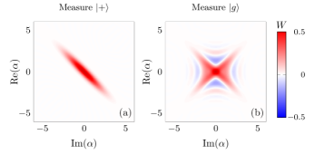
Figure 1: Wigner function heatmap of the resonator state for the case of $n=2$ when measuring the qubit in the dressed vs the bare bases. The resonator state (after a qubit measurement) generated by Eq. (10) after time-evolution period of $g_{2}t/2\pi=0.15$ for an initial state $\ket{g}\ket{0}$. The parameters used are $g_{2}=2\pi\times$20\text{\,}\mathrm{MHz}$$, and $\Delta=\delta_{2}=0$. (a) The resonator is left in a single well-defined squeezed state when the qubit is measured in the dressed basis. (b) On on the other hand, it is left in a superposition of orthogonally squeezed states when the qubit is measured in the bare basis.

When $n=2$, the time-evolution operator generated by Eq. (7) is

$$\hat{U}_{\text{eff}}^{(I)}(t,0)=\outerproduct{\overline{+}}{\overline{+}}\hat{S}(\zeta(t))+\outerproduct{\overline{-}}{\overline{-}}\hat{S}(-\zeta(t)),$$ (10)

where $\hat{S}(\zeta)=\exp((\zeta^{*}\hat{a}^{2}-\zeta\hat{a}^{\dagger 2})/2)$ is the squeezing operator and $\zeta(t)=\overline{g}_{2}(e^{i2\delta_{2}t}-1)/2\delta_{2}$ is the squeezing parameter; when $\delta_{2}\rightarrow 0$, $\zeta(t)=i\overline{g}_{2}t$. For simplicity, we henceforth assume $\Delta=0$ such that $\ket{\overline{\pm}}=\ket{\pm}$ . When the system is initialized with the qubit in the ground state and the resonator in vacuum, $\ket{\psi_{\text{i}}}=\ket{g}\ket{0}=(\ket{+}+\ket{-})\ket{0}/\sqrt{2}$, the time-evolved state reads

$$\ket{\psi(t)}^{(I)}= \frac{1}{\sqrt{2}}(\ket{+}\ket{\zeta(t)}+\ket{-}\ket{-\zeta(t)})$$

$$= \frac{1}{2}\ket{g}(\ket{\zeta(t)}+\ket{-\zeta(t)})$$

$$+\frac{1}{2}\ket{e}(\ket{\zeta(t)}-\ket{-\zeta(t)}),$$ (11)

where $\ket{\zeta}=\hat{S}(\zeta)\ket{0}$ is a squeezed vacuum state. If the qubit is measured in the basis $\{\ket{g},\ket{e}\}$, the resonator state becomes a Schrödinger-cat-like superposition of orthogonally (opposite phase) squeezed states $\propto\ket{\zeta(t)}\pm\ket{-\zeta(t)}$ with the sign depending on the measured qubit state. The Wigner function of the resonator state after measuring the qubit state in different bases is shown in Fig. 1. When the resonator is in a superposition of orthogonally squeezed states, its Wigner function dips to negative values in various regions of phase space, as shown in Fig. 1(b), thus making it a useful resource for non-Gaussian quantum computation [45]. The statistical and interference properties of general superpositions of squeezed states with different phases have been previously examined [46]. More recently, these states have been proposed as a resource for generating of heralded single photons [47].

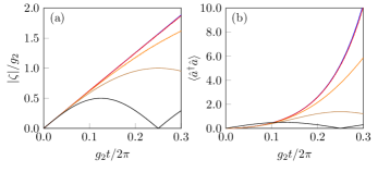
Figure 2: Dynamics of the squeezing parameter and photon number over time. The values of $\delta_{2}$ used are $\delta_{2}=2g_{2}$ (brown), $\delta_{2}=g_{2}$ (brown), $\delta_{2}=0.5g_{2}$ (orange), $\delta_{2}=0.1g_{2}$ (red) and $\delta_{2}=0$ (blue). For a fixed value of $g_{2}$, the squeezing and, consequently, the photon number grow larger in time as $\delta_{2}$ goes to zero.

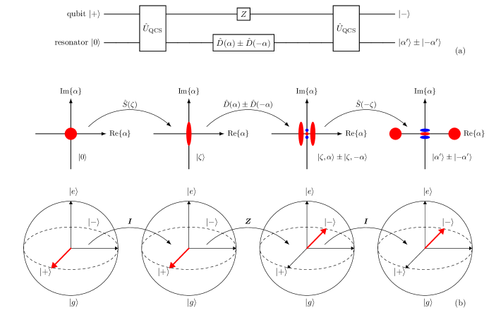
Figure 3: Cat-state amplification schematic using the phase-space and Bloch sphere pictures of the resonator and qubit, respectively. (a) Quantum circuit schematic showing the required operations for amplification. Note that this is the same scheme that amplifies a single displacement by replacing $\hat{D}(\alpha)\pm\hat{D}(-\alpha)$ with $\hat{D}(\alpha).$ (b) Effect of the steps in the circuit schematic on the phase-space picture of the resonator via its Wigner function (red is positive and blue is negative), and on the Bloch-sphere picture of the qubit via the Bloch vector of its state.

As mentioned above, when the qubit driving is two-photon-cross-resonant with the resonator ($\delta_{2}=0$), the squeezing parameter, $\zeta$, grows linearly in time. This leads to an exponential growth of the resonator photon number in time,

$$\bra{\pm\zeta(t)}\hat{a}^{\dagger}\hat{a}\ket{\pm\zeta(t)}=\sinh^{2}(\overline{g}_{2}t).$$ (12)

Figure 2 displays how the squeezing parameter and photon number change as a function of time for a fixed $\overline{g}_{2}$ and varying $\delta_{2}$. When $\delta_{2}\ll\overline{g}_{2}$, $\zeta$ behaves similarly to the two-photon-cross-resonant case.

Henceforth, we refer to the procedure of applying Eq. (10) as the QCS protocol. Interestingly, this protocol allows for the encoding of an arbitrary qubit state in a superposition of orthogonally squeezed states, akin to how qubit states can be encoded using coherent states in bosonic cat codes [48, 49, 50]. We prepare an arbitary qubit state in the $\{\ket{+},\ket{-}\}$ basis, $\ket{\psi_{q}}=c_{g}\ket{+}+c_{e}\ket{-}$ ($|c_{g}|^{2}+|c_{e}|^{2}=1$) and we initialize the resonator in vacuum. Then, we apply the QCS protocol such that the final joint state reads

$$\ket{\psi_{f}}=c_{g}\ket{+}\ket{\zeta}+c_{e}\ket{-}\ket{-\zeta}.$$ (13)

Measuring the qubit in the bare basis $\{\ket{g},\ket{e}\}$ leaves the resonator in a state $\propto c_{g}\ket{\zeta(t)}\pm c_{e}\ket{-\zeta(t)}$. As a result, the qubit state is now encoded in a superposition of orthogonally squeezed states . We now provide an alternative view of the state in Eq. (13). If the resonator is measured through its second moment $\propto(\hat{a}^{\dagger}+\hat{a})^{2}$ which is the square of the typically measured output voltage, we find one of the orthogonally squeezed states, and the qubit state is inferred from the axis of squeezing. This serves as a quantum-non-demolition (QND) measurement of the qubit through the resonator. Squeezing has been previously applied to the widely-used dispersive readout [52]. It reportedly shows significant improvements in the signal-to-noise ratio as well as a reduction in the measurement-induced dephasing. Therefore, our QCS protocol can also be used with the dispersive readout, where the benefits of unconditional squeezing will apply.

II.3.2 Amplification of displacements

The aforementioned exponential photon growth rate in the case of two-photon-cross-resonant driving can be leveraged for a fast amplification of resonator states. To this end, we prepare the system in $\ket{+}\ket{0}$, and we perform the QCS protocol using Eq. (10) to yield the state, $\ket{+}\ket{\zeta}$, where we drop the time dependence and keep it implicit. Next, we drive the resonator with a microwave field displacing the resonator state along the axis orthogonal to the axis of squeezing, leaving the system in $\ket{+}\ket{\zeta,\alpha}=\ket{+}\hat{D}(\alpha)\hat{S}(\zeta)\ket{0}$. For amplification, we now seek to ‘anti-squeeze’ the resonator, i.e., apply $\hat{S}^{\dagger}(\zeta)$. This can be done by first applying a phase flip to the qubit state such that the system is in now in $\ket{-}\ket{\zeta,\alpha}$. Alternatively, it can be done by changing the phase of the qubit drive. Then, we apply the QCS protocol again (for the same value of $\zeta$) which results in the state $\ket{-}\ket{\alpha^{\prime}}$. Here, $|\alpha^{\prime}|=G|\alpha|$ with $G=\exp(|\zeta|)=\exp(\overline{g}_{2}\tau)>0$ being the gain and $\tau$ being the time period the QCS protocol is applied in squeezing and anti-squeezing the resonator, where we use the identities $\hat{S}(-\zeta)=\hat{S}^{\dagger}(\zeta)$ and $\hat{S}^{\dagger}(\zeta)\hat{D}(\alpha)\hat{S}(\zeta)=\hat{D}(\alpha^{\prime})$ with $\alpha^{\prime}=\alpha\cosh(|\zeta|)-\alpha^{*}e^{i\arg(\zeta)}\sinh(|\zeta|)$. The final displacement on the resonator is now amplified compared to the original displacement [53].

The amplification of a single displacement is a simple example that can be generalized to amplify superpositions of displacements such as those used in generating cat states – superpositions of coherent states with different phases. It will still be true that the amplification is maximized when the squeezing and displacement axes are orthogonal, thus, we consider superpositions of collinear displacements. Here, we assume access to a cat-state-preparation method relying on an auxiliary system such as a qubit to generate a superposition of displacements [36, 37, 38]. It is possible to use the same qubit for the cat-state preparation and amplification if the qubit simultaneously interacts with the resonator via one- and two-photon interactions. We can tune the qubit to be one-photon resonant and perform qubit-conditional displacements (Eq. (7) with $n=1$) during which the two-photon interaction can be neglected. Next, we can tune the qubit to be two-photon resonant and perform the amplification scheme.

In the resonator phase space, the cat-state preparation can be seen as applying a superposition of opposite phase displacements, $\hat{D}(\alpha)\pm\hat{D}(-\alpha)$, and the QCS protocol can be seen as applying $\hat{S}(\pm\zeta)$ with the sign depending on the dressed qubit states $\ket{\pm}$. We drop normalizations for notational convenience. We perform the same steps from the single displacement amplification and, instead of applying a displacement, we now use an auxiliary system to generate a cat state in the direction orthogonal to squeezing (for maximum amplification) in the resonator which leaves the qubit-resonator system in $\ket{+}(\hat{D}(\alpha)\pm\hat{D}(-\alpha))\ket{\zeta}=\ket{+}(\ket{\zeta,\alpha}\pm\ket{\zeta,-\alpha})$. Then, as in the single displacement case, we apply a phase flip to the qubit followed by the QCS operation where the system is in $\ket{-}(\ket{\alpha^{\prime}}\pm\ket{-\alpha^{\prime}})$, where $|\alpha^{\prime}|=G|\alpha|$ with $G$ being the same gain as before. Figure 3(a) shows a quantum circuit schematic summarizing the amplification steps, while Fig. 3(b) displays the effect at each step in the phase-space and Bloch-sphere pictures of the resonator and qubit, respectively.

III Engineering Effective $n$-photon Rabi Hamiltonian with Arbitary Coupling Strength

The $n$-photon Jaynes-Cummings Hamiltonian introduced in Eq. (1) is often an excellent approximation, for weak coupling, of the more general $n$-photon Rabi model. The main difference is the presence or absence of the counter-rotating interaction terms, $\propto\hat{\sigma}_{+}\hat{a}^{\dagger n}+\hat{\sigma}_{-}\hat{a}^{n}$. We now use an additional qubit drive on the system to arrive at an effective $n$-photon Rabi model with arbitary coupling strengths, allowing the access to regimes that are currently unachievable in experimental settings [54].

We relabel the drive parameters to distinguish the two drives considered; each drive is characterized by a strength $\Omega_{k}$ and a driving frequency $\omega_{dk}$ with $k=1,2$. We start by considering the Hamiltonian of Eq. (II.1) in the presence of the two drives, which reads

$$\hat{\widetilde{H}}^{r}_{\text{RWA}}= \frac{\hbar\Delta}{2}\hat{\sigma}_{z}+\frac{\hbar\Omega_{1}}{2}\hat{\sigma}_{x}+\hbar\delta_{n}\hat{a}^{\dagger}\hat{a}$$

$$+\hbar g_{n}(\hat{\sigma}_{+}\hat{a}^{n}+\hat{\sigma}_{-}\hat{a}^{\dagger n})$$

$$+\frac{\hbar\Omega_{2}}{2}(e^{i\delta_{d}t}\hat{\sigma}_{+}+e^{-i\delta_{d}t}\hat{\sigma}_{-}),$$ (14)

where $\Delta=\omega_{q}-\omega_{d1}$, $\delta_{n}=\omega_{r}-\omega_{d1}/n$ and $\delta_{d}=\omega_{d1}-\omega_{d2}$. Here, we note that the Hamiltonian is in the rotating frame with respect to $\omega_{d1}$. Both drives are operated within the RWA regime, where

$$\Omega_{k}\ll\omega_{dk}.$$

In this setup, we seek to obtain three tunable terms in the effective Hamiltonian; qubit, resonator and interaction terms. The importance of the second drive is that it introduces a qubit term in the final effective Hamiltonian. To elucidate how the second drive plays this role, we make another transformation to the interaction picture with respect to the $\hat{\sigma}_{x}$ term in Eq. (III) via $\hat{U}^{(I)}=\exp[-i\hat{H}_{0}t/\hbar]$, where $\hat{H}_{0}=\hbar\Omega_{1}\hat{\sigma}_{x}/2$. This frame is chosen on the basis that we operate in the strong driving regime of the first drive, where $\Omega_{1}$ is the largest energy scale in Eq. (III). In this interaction picture, the system Hamiltonian reads

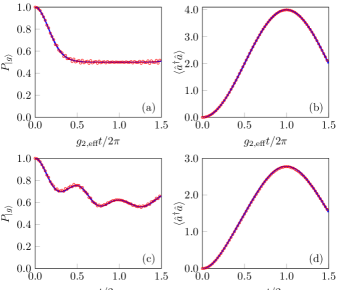
Figure 4: Quantum simulation of the two-photon Rabi model in the ultrastrong coupling regime. The time-evolution of the ground state probablity and the resonator photon number are shown for a system initialized in $\ket{g}\ket{0}$. The blue solid line is generated by Eq. (III) and the red circles are generated by Eq. (III). The parameters used are $\Omega_{1}=\delta_{d}=2\pi\times$1.4\text{\,}\mathrm{GHz}$$, $\Delta=2\pi\times$20\text{\,}\mathrm{MHz}$$, $g_{2,\text{eff}}=2\pi\times$10\text{\,}\mathrm{MHz}$$, $\omega_{r,\text{eff}}=2\pi\times$10\text{\,}\mathrm{MHz}$$. For (a),(b) $\omega_{q,\text{eff}}=0$ and for (c),(d) $\omega_{q,\text{eff}}=2\pi\times$10\text{\,}\mathrm{MHz}$$.

$$\hat{H}^{(I)}= -\frac{\hbar\Delta}{2}(e^{i\Omega_{1}t}\outerproduct{+}{-}+e^{-i\Omega_{1}t}\outerproduct{-}{+})+\hbar\delta_{n}\hat{a}^{\dagger}\hat{a}$$

$$+\frac{\hbar}{2}\Bigg{[}\bigg{(}\outerproduct{+}{+}-\outerproduct{-}{-}+e^{i\Omega_{1}t}\outerproduct{+}{-}$$

$$-e^{-i\Omega_{1}t}\outerproduct{-}{+}\bigg{)}\bigg{(}g_{n}\hat{a}^{n}+\frac{\Omega_{2}}{2}e^{i\delta_{d}t}\bigg{)}+\text{H.c.}\Bigg{]}.$$ (15)

As discussed in Sec. II.2.1, with $\Omega_{1}$ as the dominant energy scale, we explicitly impose $\Omega_{1}\gg|\Delta|,g_{n}$. This assumption enables us to disregard the rapidly oscillating terms with factors of $e^{\pm i\Omega_{1}t}$. Next, we set $\delta_{d}=\Omega_{1}$, which cancels the time dependence in the terms responsible for the effective qubit term, $-(\outerproduct{-}{+}e^{i(\delta_{d}-\Omega_{1})t}+\text{H.c.})$. Note that the term $(\outerproduct{+}{-}e^{i(\delta_{d}+\Omega_{1})t}+\text{H.c.})$ oscillates with $e^{\pm i(\delta_{d}+\Omega_{1})t}$ and can therefore be ignored. This allows us to obtain an effective $n$-photon Rabi Hamiltonian

$$\hat{H}_{\text{eff}}^{(I)}= -\frac{\hbar\Omega_{2}}{4}(\outerproduct{+}{-}+\outerproduct{-}{+})+\hbar\delta_{n}\hat{a}^{\dagger}\hat{a}$$

$$+\frac{\hbar g_{n}}{2}(\outerproduct{+}{+}-\outerproduct{-}{-})(\hat{a}^{\dagger n}+\hat{a}^{n})$$

$$= \frac{\hbar\omega_{q,\text{eff}}}{2}\hat{\sigma}_{z}+\hbar\omega_{r,\text{eff}}\hat{a}^{\dagger}\hat{a}$$

$$+\hbar g_{n,\text{eff}}\hat{\sigma}_{x}(\hat{a}^{\dagger n}+\hat{a}^{n}),$$ (16)

where $\omega_{q,\text{eff}}=\Omega_{2}/2$, $\omega_{r,\text{eff}}=\delta_{n}$ and $g_{n,\text{eff}}=g_{n}/2$. Here, we have rewritten the Hamiltonian in the bare basis where $\hat{\sigma}_{x}=\hat{\sigma}_{+}+\hat{\sigma}_{-}=\outerproduct{+}{+}-\outerproduct{-}{-}$ and $\hat{\sigma}_{z}=-(\outerproduct{+}{-}+\outerproduct{-}{+})/2$. The effective system parameters are highly tunable and allow for a quantum simulation of the $n$-photon Rabi model in various coupling regimes. Note that when $\Omega_{2}=0$ (i.e. in the absence of the second drive), Eq. (III) is the same as Eq. (8) with the only difference being a transformation with respect to the resonator term via $\exp(i\delta_{n}t\hat{a}^{\dagger}\hat{a})$. Therefore, in the case of $\Omega_{2}=0$, we recover the results of Sec. II.2.1.

In the multiphoton generalizations of the Rabi model, the phenomenon of spectral collapse occurs at stronger coupling regimes where $g_{n,\text{eff}}$ is comparable to (or larger than) $\omega_{q,\text{eff}}$ and $\omega_{r,\text{eff}}$. Thus, an effective Hamiltonian with tunable parameters allows us to probe the dynamical behaviour in such extreme scenarios. Figure 4 shows the dynamics of the effective Hamiltonian in Eq. (III) compared to Eq. (III) for the case $n=2$ in the ultrastrong coupling regime $g_{2,\text{eff}}/\omega_{r,\text{eff}}\simeq 0.1$. As the amplitude $\Omega_{1}$ increases, the effective and full Hamiltonian dynamics get closer to each other. Even for experimentally realistic drive strengths (Fig. 4 uses $\Omega_{1}=2\pi\times$1.4\text{\,}\mathrm{GHz}$$), the dynamics of the full Hamiltonian with the same parameters very closely resembles that of the effective model.

Increasing the native coupling strength of the system – as we will see in the next section – typically comes with an increase in the strength of spurious terms that may completely ruin the desired interaction. Thus, engineering effective Hamiltonians in extreme parameter regimes using appropriately designed driving fields allows for achieving experimentally inaccessible regimes using easily accessible coupling strengths.

IV Circuit QED implementation

While the experiments proposed in Secs. II.3 and III are implementation independent, we are interested in circuit QED as an implementation platform due to the range of coupling strengths it can achieve and its potential for scalability. There are two proposals in the literature for a circuit implementation of the two-photon Rabi model; a flux qubit inductively coupled to a superconducting quantum interference device (SQUID) [28, 33] and a split-Cooper-pair-box (charge qubit) inductively coupled to a transmission line [30]. In fact, the use of a (dc or rf) SQUID as a tunable coupler has long been known (see e.g. Refs. [55, 56]), even though employing it to obtain nonperturbative nonlinear interactions is fairly recent [40, 57].

Figure 5: Transmon coupled to a resonator via an asymmetric SQUID. The transmon is characterized by a Josephson energy $E_{Jt}$ and charging energy $E_{Ct}=2e/(C_{Jt}+C_{t})$ depending on the junction and shunt capactiance; $E_{Jt}/E_{Ct}$ for this device is above 50 to operate in the transmon regime. The asymmetric SQUID has differing Josephson energies, $E_{J1}$ and $E_{J2}$, to exclusively allow for odd-order terms. The flux degrees of freedom are shown for the transmon, $\phi_{t}$, resonator, $\phi_{r}$, and the SQUID (coupler), $\phi_{1}$ and $\phi_{2}$. The coupler degrees of freedom are a function of the transmon, resonator and external flux threading the SQUID.

Here, we propose to employ the more widely used transmon qubit [58] coupled to a lumped-element LC resonator via an asymmetric DC-SQUID threaded with an external flux, as shown in Fig. 5. The circuit Hamiltonian is (see App. B for a detailed derivation)

$$\hat{H}= \frac{\hat{q}_{t}^{2}}{2\overline{C}_{t}}-E_{Jt}\cos(\frac{2\pi\hat{\phi}_{t}}{\phi_{0}})+\frac{\hat{q}_{r}^{2}}{\overline{C}_{r}}+\frac{\hat{\phi}_{r}^{2}}{2L_{r}}+\frac{1}{\overline{C}_{c}}\hat{q}_{t}\hat{q}_{r}$$

$$-E_{c}\cos(\frac{2\pi(\hat{\phi}_{t}-\hat{\phi}_{r})}{\Phi_{0}})$$

$$-E_{s}\sin(\frac{2\pi(\hat{\phi}_{t}-\hat{\phi}_{r})}{\Phi_{0}}).$$ (17)

where $\Phi_{0}$ is the magnetic flux quantum, $\Phi_{\text{ext}}$ is the external flux threading the SQUID, and $\hat{\phi}_{k}$ and $\hat{q}_{k}$ are subsystem $k$’s flux and charge operators with $k=r$ referring to the resonator and $k=t$ referring to the transmon. The transmon is characterized by a Josephson energy $E_{Jt}$ and total (renormalized) capacitance $\overline{C}_{t}$, while the resonator is characterized by an inductance $L_{r}$ and (renormalized) capacitance $\overline{C}_{r}$. Finally, the SQUID coupler is characterized by asymmetric Josephson junctions with energies $E_{J1}$ and $E_{J2}$ dictacting effective coupler energies $E_{c}=E_{J1}\cos(2\pi\Phi_{\text{ext}}/{\Phi_{0}})+E_{J2}$ and $E_{s}=E_{J1}\sin({2\pi\Phi_{\text{ext}}}/{\Phi_{0}})$. We assume that $E_{J1}\geq E_{J2}$. The asymmetry is necessary to exclusively generate odd-order qubit-resonator interactions, i.e., interactions of the form $\hat{\phi}_{t}^{j}\hat{\phi}_{r}^{k}$ where $j+k$ is an odd integer. We set $\Phi_{\text{ext}}=\Phi_{0}\arccos(-E_{J2}/E_{J1})/2\pi$, thus, making $E_{c}=0$ such that the even order interactions are completely cancelled. This results in a purely odd-order interaction. The two-photon JC interaction is classified under odd-order terms, generated by $\hat{\phi}_{t}\hat{\phi}_{r}^{2}$. When the qubit and resonator zero-point-fluctuation flux values are small, we may truncate the sine term, $\sin({2\pi(\hat{\phi}_{t}-\hat{\phi}_{r})}/{\Phi_{0}})$, at third order. Since the transmon is anharmonic and we assume the transition between the ground and first excited states to be the only resonant transition, the dynamics are confined to the lowest two energy eigenstates. Therefore, we also employ the two-level approximation (TLA) such that the circuit QED Hamiltonian reads

Table 1: Circuit and Hamiltonian parameter estimates for operating a transmon coupled to a resonator via an asymmetric SQUID in the two-photon Jaynes-Cummings regime.

Parameter	Two-photon mode
$\omega_{q}$	$2\pi\times$$10\text{\,}\mathrm{GHz}$
$E_{Jt}/\hbar$	$2\pi\times$$86.5\text{\,}\mathrm{GHz}$
$E_{Ct}/\hbar$	$2\pi\times$$150\text{\,}\mathrm{MHz}$
$\omega_{r}$	$2\pi\times$$5\text{\,}\mathrm{GHz}$
$C_{r}$	$330\text{\,}\mathrm{fF}$
$E_{J1}/\hbar$	$2\pi\times$10.00-$18.00\text{\,}\mathrm{GHz}$
$E_{J2}/\hbar$	$2\pi\times$9.94-$17.50\text{\,}\mathrm{GHz}$
$g_{2}$	$2\pi\times$25-$50\text{\,}\mathrm{MHz}$
$\widetilde{g}_{e1}$	$2\pi\times$1.08-$2.16\text{\,}\mathrm{GHz}$
$\widetilde{g}_{e2}$	$2\pi\times$1.34-$2.68\text{\,}\mathrm{GHz}$
$\widetilde{g}_{e3}$	$2\pi\times$5-$10\text{\,}\mathrm{MHz}$
$\widetilde{g}_{e4}$	$2\pi\times$10-$40\text{\,}\mathrm{MHz}$
$\widetilde{g}_{e5}$	$2\pi\times$20-$80\text{\,}\mathrm{MHz}$
$\widetilde{g}_{c}$	$2\pi\times$30-$50\text{\,}\mathrm{MHz}$

$$\hat{H}^{\text{TLA}}= \frac{\hbar\omega_{q}}{2}\hat{\sigma}_{z}+\hbar\omega_{r}\hat{a}^{\dagger}\hat{a}-\hbar\widetilde{g}_{e4}(\hat{a}^{\dagger}+\hat{a})^{3}$$

$$-\hbar\widetilde{g}_{e5}\hat{\sigma}_{z}(\hat{a}^{\dagger}+\hat{a})+\hbar g_{2}(\hat{\sigma}_{+}+\hat{\sigma}_{-})(\hat{a}^{\dagger}+\hat{a})^{2}$$

$$-\hbar\widetilde{g}_{c}(\hat{\sigma}_{+}-\hat{\sigma}_{-})(\hat{a}^{\dagger}-\hat{a}),$$

$$-\hbar(\widetilde{g}_{e1}-\widetilde{g}_{e3})(\hat{\sigma}_{+}+\hat{\sigma}_{-})$$

$$-\hbar(2\widetilde{g}_{e5}-\widetilde{g}_{e2})(\hat{a}^{\dagger}+\hat{a}),$$

where $\widetilde{g}_{e1},\,\widetilde{g}_{e2}\,\widetilde{g}_{e3},\,\widetilde{g}_{e4}$ and $\widetilde{g}_{e5}$ are spurious inductive couplings and $\widetilde{g}_{c}$ is a spurious capactive coupling. Here, $\omega_{q}=\sqrt{8E_{Ct}E_{Jt}}-E_{Ct}$ and $\omega_{r}=1/\sqrt{L_{r}\overline{C}_{r}}$. We now proceed to simplify this model to achieve the two-photon JC Hamiltonian. First, we neglect the linear offset terms, $\propto\hat{\sigma}_{+}+\hat{\sigma}_{-}$ and $\propto\hat{a}^{\dagger}+\hat{a}$, as they can be tuned to zero in-situ by applying a microwave field, and, thus, the tuned circuit QED Hamiltonian reads

$$\hat{H}^{\text{TLA}}= \frac{\hbar\omega_{q}}{2}\hat{\sigma}_{z}+\hbar\omega_{r}\hat{a}^{\dagger}\hat{a}-\hbar\widetilde{g}_{e4}(\hat{a}^{\dagger}+\hat{a})^{3}$$

$$-\hbar\widetilde{g}_{e5}\hat{\sigma}_{z}(\hat{a}^{\dagger}+\hat{a})+\hbar g_{2}(\hat{\sigma}_{+}+\hat{\sigma}_{-})(\hat{a}^{\dagger}+\hat{a})^{2}$$

$$-\hbar\widetilde{g}_{c}(\hat{\sigma}_{+}-\hat{\sigma}_{-})(\hat{a}^{\dagger}-\hat{a}).$$ (18)

We now assume the two-photon JC conditions

$$2\omega_{r}=\omega_{q}\text{ and }g_{2}\ll\omega_{r}.$$ (19)

With these conditions, only the two-photon JC terms are resonant, while all the other terms are off-resonant and can be neglected (see App. B for details). Then, the effective circuit QED Hamiltonian becomes

$$\hat{H}^{\text{TLA}}\simeq\frac{\hbar\omega_{q}}{2}\hat{\sigma}_{z}+\hbar\omega_{r}\hat{a}^{\dagger}\hat{a}-\hbar g_{2}(\hat{\sigma}_{+}\hat{a}^{2}+\hat{\sigma}_{-}\hat{a}^{\dagger 2}).$$ (20)

This final Hamiltonian shows that the proposed circuit has the necessary two-photon qubit-resonator interaction required to host the QCS protocol (and its subsequent applications) and to obtain an effective two-photon Rabi Hamiltonian at arbitrary coupling strengths.

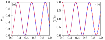
Figure 6: Two-photon Rabi oscillations exhibited in the dynamics of the qubit excited state probability and resonator photon number for an initial state $\ket{g}\ket{2}$. The blue lines are generated by the two-photon Jaynes-Cummings Hamiltonian in Eq. (20) and the red lines are generated by the two-level approximation circuit QED Hamiltonian in Eq. (IV).

In Table 1, we provide realistic experimental parameters of the proposed circuit that can achieve the two-photon JC interaction. The details of the spurious couplings and their relations to the physical circuit parameters are derived in detail in App. B. We perform numerical simulations of the circuit QED model including spurious couplings using our estimated parameters to validate the two-photon JC interaction. Figure 6 shows the dynamics generated using Eq. (IV) contrasted to those generated using Eq. (20). The probability of the excited state and the resonator photon number are shown as they evolve in time starting from an initial state $\ket{g}\ket{2}$. The circuit QED model exhibits two-photon Rabi oscillations in in excellent agreement with the ideal model.

The asymmetry of the SQUID we rely on here has also been used to implement multiphoton spontaneous parametric down conversion (SPDC) between bosonic modes [59, 40, 57, 32, 60]. The proposed device here is based on the same principles used for multiphoton SPDC with the difference being that we are coupling a bosonic mode to a transmon effectively truncated to its two lowest energy eigenstates. Our proposal can be used to reach the two-photon near-resonance strong coupling regime, i.e., $g_{2}\gg\kappa,\gamma_{1},\gamma_{\phi}$ and $\omega_{q}\simeq 2\omega_{r}$, where $\kappa$ is the resonator photon loss rate, $\gamma_{1}$ is the qubit relaxation rate and $\gamma_{\phi}$ is the qubit dephasing rate. The potential use for an asymmetric SQUID is not limited to the two-photon interactions. In fact, we have already investigated this same circuit for a three-photon qubit-resonator interaction; it can be adapted to tune the SQUID interaction, which in this case significantly renormalizes the qubit and resonator frequencies, and introduces resonant spurious couplings that need careful management. The details of a three-photon implementation will be published elsewhere.

V Summary and Conclusions

To summarize, we presented a general theory on driving-enhanced $n$-photon qubit-resonator interactions. The multiphoton interactions are generated in the strong and qubit-detuned weak driving regimes with $n$-photon cross-resonance yielding the highest rate of channeling photons into the resonator. After developing the general framework, we focused on the case of $n=2$, where the theory yields qubit-conditional squeezing (QCS). Then, we described how the QCS protocol can be used in encoding a qubit state in the superposition of orthogonally squeezed states. We also showed how to perform a QND measurement of the qubit via QCS. Additionally, we outlined a scheme that amplifies displacements (single and a superposition of them) using QCS.

After exploring the regimes of the driving-enhanced interactions and their applications for the case of $n=2$, we explored the use of two drives to obtain an effective $n$-photon Rabi Hamiltonian with arbitrary coupling strength. When the first drive is the largest energy scale, we showed that the second drive plays the role of the qubit term in the effective Hamiltonian. While, the detuning between the first drive and the resonator served as the effective resonator frequency. Interestingly, the effective qubit-resonator $n$-photon coupling is given by the native coupling strength and is independent of the drive parameters.

From the implementation side, the generation of nonperturbative $n$-photon qubit-resonator interactions beyond $n=1$ is a challenging task. First, one major difficulty lies in obtaining a Hamiltonian where the $n^{\text{th}}$ order interaction can be isolated without the presence of spurious terms of comparable coupling strength. Second, the coupling strength in most systems significantly diminishes as the order of the interaction increases. Therefore, even if it is possible to obtain a Hamiltonian with the desired interaction, we require the strong coupling regime, i.e., $g_{n}\gg\kappa,\,\gamma_{1},\,\gamma_{\phi}$. Without satisfying these conditions, the system will be dominated by losses, rendering the sought effects incoherent and suppressed by the system’s losses. Here, we proposed an implementation that can achieve the necessary conditions for our theory in the case of $n=2$. The circuit uses a transmon qubit coupled to a lumped-element LC resonator by means of an asymmetric SQUID. We provided realistic experimental parameters and validated the circuit QED model using numerical simulations exhibiting two-photon Rabi oscillations.

Throughout the paper, we exclusively discussed unitary evolution. In App. A, we perform extensive open system numerical simulations for worse-than-average decoherence qubit and resonator parameters and corroborate the analytical results; the predictions are robust against qubit energy relaxation and dephasing and resonator photon loss. We find the fidelity of the states generated to be largely unaffected at the timescales of consideration used in the paper.

This work paves the way for a new set of nonperturbative multiphoton qubit-resonator effects that can be leveraged for applications in various quantum applications for information processing — as presented here, sensing, and communication.

Appendix A Decoherence

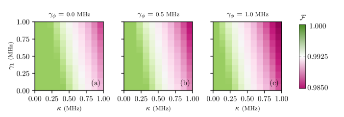
Figure 7: Fidelity of prepared state with varying decoherence rates. The Hamiltonian parameters and initial state used for the simulations are $\Omega=2\pi\times$0.5\text{\,}\mathrm{GHz}$$, $g_{2}=2\pi\times$20\text{\,}\mathrm{MHz}$$, and $\Delta=\delta_{2}=0$ (identical to those in Fig. 1 in the main text with the decoherence parameters varied). (a)-(c) The fidelity between a state prepared via time-evolution using Eq.(21) and a reference state evolved with Eq.(1) is plotted for different qubit and resonator decoherence rates, with a time-evolution period of $g_{2}t/2\pi=0.3$. The resonator photon loss rate, $\kappa$, is the most detrimental parameter to the state fidelity. The qubit relaxation rate, $\gamma_{1}$, also diminishes the fidelity but the qubit dephasing, $\gamma_{\phi}$, is practically negligible as the three plots are nearly identical.

We only considered unitary time evolution in the main text. The qubit-resonator system are not completely isolated from the environment. Here, we take into account qubit energy relaxation, qubit dephasing and resonator photon loss. Since we are operating in the strong coupling regime, the qubit and resonator are not strongly hybradized and, thus, we can assume they interact with separate baths at zero temperature. For these conditions, it suffices to model the open system using a Lindblad master equation that reads [61, 62]

$$\frac{d}{dt}\hat{\rho}=-\frac{i}{\hbar}[\hat{H},\hat{\rho}]+\gamma_{1}\mathcal{D}(\hat{\sigma}_{-})\hat{\rho}+\frac{\gamma_{\phi}}{2}\mathcal{D}(\hat{\sigma}_{z})\hat{\rho}+\kappa\mathcal{D}(\hat{a})\hat{\rho},$$ (21)

where $\hat{\rho}$ is the full system density matrix, $\mathcal{D}(\hat{O})\hat{\rho}=\hat{O}\hat{\rho}\hat{O}^{\dagger}-\{\hat{O}^{\dagger}\hat{O},\hat{\rho}\}/2$ is the dissipator for a given operator $\hat{O}$, $\gamma_{1}$ and $\gamma_{\phi}$ are the qubit energy relaxation and dephasing rates, and $\kappa$ is the resonator photon loss rate. In what follows we use the Python library QuTiP [63]

We seek to evaluate the contribution of different decoherence parameters on the prepared state, $\hat{\rho}_{\text{prep}}$. For that purpose, we define the fidelity as

$$\mathcal{F}=\left(\Tr(\sqrt{\sqrt{\hat{\rho}_{\text{prep}}}\hat{\rho}_{\text{ideal}}\sqrt{\hat{\rho}_{\text{prep}}}})\right)^{2},$$

where we use an ideal reference state $\hat{\rho}_{\text{ideal}}$ obtained using Eq. (1) and $\hat{\rho}_{\text{prep}}$ is arrived at using the master equation, Eq. (21). Figure 7 demonstrates the results of numerical simulations in which both the reference and prepared states experienced time evolution over a normalized time of $g_{2}t/2\pi=0.3$. The same figure also highlights that the photon loss rate in the resonator is the most significant factor affecting the fidelity of the state. Although qubit relaxation contributes to a reduction in fidelity, the influence of qubit dephasing is almost inconsequential within this timescale. It is important to note that the maximum decoherence rates used in our simulations, set at $1\text{\,}\mathrm{MHz}$, are substantially higher than those typically found in present circuit QED setups, and even more so in state-of-the-art devices.

Note that the time-evolution period may seem short ($g_{2}t/2\pi=0.3$), but by the analytic estimate of Eq. (7) in the main text, the resonator will contain much more than 100 photons in a duration less than $g_{2}t/2\pi=0.5$. This is also apparent by the form of the squeezing parameter, $\zeta=ig_{2}t$ which grows linearly in time. Due to this fact, it is very hard to simulate long-time dynamics using traditional software packages such as QuTiP (employed here). For these simulations, we truncated the resonator Hilbert space to 150 photons. A more rigorous numerical study is needed for the study of the long-time dynamics and eventual decay of the photon number, but for the purpose of ensuring the robustness of state preparation against decoherence, the simulations here suffice to corroborate the analytical predicitions.

Appendix B Derivation of Circuit QED Implementation

In this section, we derive and quantize the system Hamiltonian for the circuit implementation proposed in the main text. We then proceed to apply the two-level approximation to the transmon along with the relevant RWA to obtain the two-photon Jaynes-Cummings Hamiltonian.

B.1 Circuit Hamiltonian

We first begin by stating the total system (transmon, resonator and coupler) Lagrangian for the circuit shown in Fig. 5. We use the system constraints to eliminate the coupler degree of freedom and express it in terms of the transmon and resonator degrees of freedom. Then, we obtain the classical Hamiltonian by means of a Legendre transformation. Then, we promote the conjugate variables to quantum operators, arriving at a quantum-mechanical description of the circuit.

The total system Lagrangian is [40]

$$\mathcal{L}_{\text{total}}=\mathcal{L}_{\text{transmon}}+\mathcal{L}_{\text{resonator}}+\mathcal{L}_{\text{coupler}},$$ (22)

where

$$\mathcal{L}_{\text{transmon}}=\frac{1}{2}C_{\Sigma}\dot{\phi}_{t}^{2}+E_{Jt}\cos(\frac{2\pi\phi_{t}}{\Phi_{0}}),$$ (23)

$$\mathcal{L}_{\text{resonator}}=\frac{1}{2}C_{r}\dot{\phi}_{r}^{2}-\frac{1}{2L_{r}}\phi_{r}^{2},$$ (24)

and

$$\mathcal{L}_{\text{coupler}}= \frac{1}{2}C_{J1}\dot{\phi}_{1}^{2}+\frac{1}{2}C_{J2}\dot{\phi}_{2}^{2}$$

$$+E_{J1}\cos(\frac{2\pi\phi_{1}}{\Phi_{0}})+E_{J2}\cos(\frac{2\pi\phi_{2}}{\Phi_{0}}).$$ (25)

Here, $\phi_{j}$ is the flux variable and $\dot{\phi}_{j}$ is its time derivative for the $j$ subsystem with $t$ denoting the transmon, $r$ denoting the resonator and 1 and 2 denoting the two junctions of the DC-SQUID coupler. The transmon is characterized by Josephson energy $E_{Jt}$ and total (junction and shunting capacitance) $C_{\Sigma}=C_{Jt}+C_{t}$. The resonator is characterized by the inductance $L_{r}$ and capacitance $C_{r}$. Lastly, the DC-SQUID is characterized by its junction capacitances $C_{J1}$ and $C_{J2}$ and Josephson energies $E_{J1}$ and $E_{J2}$.

We now derive relations between the different circuit variables and use these relations as constraints to eliminate redundant variables. Specifically, we would like to eliminate the coupler and instead obtain a Lagrangian written in terms of the transmon and resonator variables only. For this purpose, we need to examine the circuit in Fig. 5. We assume that there is no external flux applied to the loop that goes from the ground through the transmon, the bottom junction of the coupler, the resonator and back to the ground. Assuming a constant external flux, the loops are related through Kirchoff’s voltage law (KVL) constraints by:

$$\dot{\phi}_{t}-\dot{\phi}_{2}-\dot{\phi}_{r}=0$$ (26)

and

$$\dot{\phi}_{1}-\dot{\phi}_{2}=0.$$ (27)

Integrating these KVL constraints yields the flux relations

$${\phi}_{t}-{\phi}_{2}-{\phi}_{r}=\widetilde{\Phi}$$ (28)

and

$$\phi_{1}-\phi_{2}+\Phi_{\text{ext}}=\widetilde{\widetilde{\Phi}},$$ (29)

where $\tilde{\Phi}$ and $\widetilde{\widetilde{\Phi}}$ are constants of integration. In the case of a superconducting loop, these constants of integration correspond to an integer multiple of the flux quantum $\Phi_{0}$, i.e. $\widetilde{\Phi}=k_{1}\Phi_{0}$ and $\widetilde{\widetilde{\Phi}}=k_{2}\Phi_{0}$ for some integers $k_{1}$ and $k_{2}$. We now use Eqs. (29) and (27) to eliminate $\phi_{1}$ from Eq. (25) and obtain

$$\mathcal{L}_{\text{coupler}}= \frac{1}{2}(C_{J1}+C_{J2})\dot{\phi}_{2}^{2}+E_{J1}\cos(\frac{2\pi(\phi_{2}-\Phi_{\text{ext}})}{\Phi_{0}})$$

$$+E_{J2}\cos(\frac{2\pi\phi_{2}}{\Phi_{0}})$$

$$= \frac{1}{2}C_{c}\dot{\phi}_{2}^{2}+E_{c}\cos(\frac{2\pi\phi_{2}}{\Phi_{0}})+E_{s}\sin(\frac{2\pi\phi_{2}}{\Phi_{0}}),$$ (30)

where

$$C_{c}= C_{J1}+C_{J2},$$

$$E_{c}= E_{J1}\cos(\frac{2\pi\Phi_{\text{ext}}}{\Phi_{0}})+E_{J2},$$

$$E_{s}= E_{J1}\sin(\frac{2\pi\Phi_{\text{ext}}}{\Phi_{0}}).$$ (31)

Next we use Eqs. (28) and (26) to eliminate $\phi_{2}$ from Eq. (30) and obtain

$$\mathcal{L}_{\text{coupler}}= \frac{1}{2}C_{c}(\dot{\phi}_{t}-\dot{\phi}_{r})^{2}+E_{c}\cos(\frac{2\pi(\phi_{t}-\phi_{r})}{\Phi_{0}})$$

$$+E_{s}\sin(\frac{2\pi(\phi_{t}-\phi_{r})}{\Phi_{0}}).$$ (32)

The total Lagrangian can then be written as

$$\mathcal{L}=\frac{1}{2}\dot{\vec{\phi}}^{\,T}\bm{C}\dot{\vec{\phi}}-U(\vec{\phi})$$ (33)

where

$$\vec{\phi}=\begin{pmatrix}\phi_{t}\\ \phi_{r}\end{pmatrix},$$ (34)

$$\bm{C}=\begin{pmatrix}C_{t}+C_{Jt}+C_{J1}+C_{J2}&-(C_{J1}+C_{J2})\\ -(C_{J1}+C_{J2})&C_{r}+C_{J1}+C_{J2}\end{pmatrix},$$ (35)

and

$$U(\vec{\phi})= -E_{c}\cos(\frac{2\pi(\phi_{t}-\phi_{r})}{\Phi_{0}})$$

$$+E_{s}\sin(\frac{2\pi(\phi_{t}-\phi_{r})}{\Phi_{0}})$$

$$-E_{Jt}\cos(\frac{2\pi\phi_{t}}{\Phi_{0}})+\frac{1}{2L_{r}}\phi_{r}^{2}.$$ (36)

Then, the Hamiltonian can be derived via the Legendre transform as

$$H=\frac{1}{2}\vec{q}^{\,T}(\bm{C}^{-1})\vec{q}+U(\vec{\phi}),$$ (37)

where

$$\vec{q}=\begin{pmatrix}q_{t}\\ q_{r}\end{pmatrix},$$ (38)

with $q_{k}=\partial\mathcal{L}/\partial\dot{\phi}_{k}$ ($k=q,r$) being the charges stored in the qubit and resonator. We label $(\bm{C}^{-1})_{11}\equiv\overline{C}_{t}^{-1}$, $(\bm{C}^{-1})_{22}\equiv\overline{C}_{r}^{-1}$, and $(\bm{C}^{-1})_{12}=(\bm{C}^{-1})_{21}\equiv\overline{C}_{c}^{-1}$. Thus, the Hamiltonian can be written as

$$H= \frac{q_{t}^{2}}{2\overline{C}_{t}}-E_{Jt}\cos(\frac{2\pi\phi_{t}}{\phi_{0}})+\frac{q_{r}^{2}}{\overline{C}_{r}}+\frac{\phi_{r}^{2}}{2L_{r}}+\frac{1}{\overline{C}_{c}}q_{t}q_{r}$$

$$-E_{c}\cos(\frac{2\pi(\phi_{t}-\phi_{r})}{\Phi_{0}})$$

$$+E_{s}\sin(\frac{2\pi(\phi_{t}-\phi_{r})}{\Phi_{0}}).$$ (39)

Finally, we promote the classical Poisson brackets to commutator brackets via the rule

$$\{\phi_{t},q_{t}\}\mapsto[\hat{\phi}_{t},\hat{q}_{t}]=i\hbar,$$

$$\{\phi_{r},q_{r}\}\mapsto[\hat{\phi}_{r},\hat{q}_{r}]=i\hbar,$$

where $\hat{q}_{k},\,\hat{\phi}_{k}$ are now quantized operators. By reeplacing the variables with operators, we obtain the quantum circuit Hamiltonian in Eq. (IV).

For the derivations to follow, we isolate the inductive and capacitive SQUID interactions from the total Hamiltonian. The inductive SQUID interaction Hamiltonian we refer to is

$$\hat{H}_{I,\text{SQ}}^{\text{ind}}= -E_{c}\cos(\frac{2\pi(\hat{\phi}_{t}-\hat{\phi}_{r})}{\Phi_{0}})$$

$$-E_{s}\sin(\frac{2\pi(\hat{\phi}_{t}-\hat{\phi}_{r})}{\Phi_{0}}).$$ (40)

While, the capacitive SQUID interaction Hamiltonian is

$$\hat{H}_{I,\text{SQ}}^{\text{cap}}=\frac{1}{\overline{C}_{c}}\hat{q}_{t}\hat{q}_{r}.$$ (41)

Finally, we rewrite the qubit and resonator flux and charge operators using the bosonic creation and annihilation operators,

$$\hat{q}_{r}=iq_{\text{zpf},r}(\hat{a}^{\dagger}-\hat{a}),$$ (42a)

$$\hat{\phi}_{r}=\phi_{\text{zpf},r}(\hat{a}^{\dagger}+\hat{a}),$$ (42b)

$$\hat{q}_{t}=iq_{\text{zpf},t}(\hat{b}^{\dagger}-\hat{b}),$$ (42c)

and

$$\hat{\phi}_{t}=\phi_{\text{zpf},t}(\hat{b}^{\dagger}+\hat{b}),$$ (42d)

where $\phi_{\text{zpf},t}$ and $q_{\text{zpf},t}$ ($\phi_{\text{zpf},r}$ and $q_{\text{zpf},r}$) are the qubit (resonator) zero-point-fluctuation flux and charge values, respectively. The commutation relations for the qubit and resonator creation and annihilation operators are $[\hat{b},\hat{b}^{\dagger}]=\mathbb{I}$ and $[\hat{a},\hat{a}^{\dagger}]=\mathbb{I}$, respectively.

B.2 Two-photon Jaynes-Cummings Hamiltonian

For small zero-point-fluctuation flux values, we may Taylor-expand the sine and cosine into the first few polynomial terms. We are interested in the odd order terms to obtain an effective two-photon Jaynes-Cummings Hamiltonian. For this purpose, we now focus on the odd order terms by setting $\Phi_{\text{ext}}=\Phi_{0}\arccos(-E_{J2}/E_{J1})/2\pi$, thus, making $E_{c}=0$.

$$\hat{H}_{I,\text{SQ}}^{\text{ind}} =-E_{s}\left[\frac{2\pi(\hat{\phi}_{t}-\hat{\phi}_{r})}{\Phi_{0}}-\frac{1}{3!}\frac{8\pi^{3}(\hat{\phi}_{t}-\hat{\phi}_{r})^{3}}{\Phi_{0}^{3}}\right]$$

$$=-E_{s}\Bigg{[}\frac{2\pi}{\Phi_{0}}(\phi_{\text{zpf},t}(\hat{b}^{\dagger}+\hat{b})-\phi_{\text{zpf},r}(\hat{a}^{\dagger}+\hat{a}))-\frac{1}{3!}\frac{8\pi^{3}}{\Phi_{0}^{3}}\big{(}\phi_{\text{zpf},t}^{3}(\hat{b}^{\dagger}+\hat{b})^{3}-\phi_{\text{zpf},r}^{3}(\hat{a}^{\dagger}+\hat{a})^{3}$$

$$\,\,\,\,\,-3\phi_{\text{zpf},t}^{2}\phi_{\text{zpf},r}(\hat{b}^{\dagger}+\hat{b})^{2}(\hat{a}^{\dagger}+\hat{a})+3\phi_{\text{zpf},t}\phi_{\text{zpf},r}^{2}(\hat{b}^{\dagger}+\hat{b})(\hat{a}^{\dagger}+\hat{a})^{2}\big{)}\Bigg{]}$$ (43)

We now rearrange terms using the commutation relations, $[\hat{b},\hat{b}^{\dagger}]=\mathbb{I}$ and $[\hat{a},\hat{a}^{\dagger}]=\mathbb{I}$, and we use the two-level approximation where usually $\hat{b}\mapsto\hat{\sigma}_{-}\,\,(\hat{b}^{\dagger}\mapsto\hat{\sigma}_{+})$ and $\hat{b}^{\dagger}\hat{b}\mapsto\hat{\sigma}_{z}$, and for the higher-order terms we truncate to the two-dimensional subspace. In this case, $\hat{b}^{\dagger}+\hat{b}\simeq\hat{\sigma}_{+}+\hat{\sigma}_{-}$, $(\hat{b}^{\dagger}+\hat{b})^{2}\simeq\hat{\sigma}_{z}+2\hat{\mathbb{I}}$, $(\hat{b}^{\dagger}+\hat{b})^{3}\simeq 3(\hat{\sigma}_{+}+\hat{\sigma}_{-})$ and $(\hat{b}^{\dagger}+\hat{b})^{4}\simeq(9\hat{\sigma}_{z}+6\hat{\mathbb{I}})$. Thus, we get that

$$\hat{H}_{\text{SQ},I}^{\text{ind,TLA}} \simeq-E_{s}\Bigg{[}\frac{2\pi}{\Phi_{0}}(\phi_{\text{zpf},t}(\hat{\sigma}_{+}+\hat{\sigma}_{-}))-\frac{2\pi}{\Phi_{0}}(\phi_{\text{zpf},r}(\hat{a}^{\dagger}+\hat{a}))-\frac{1}{3!}\frac{8\pi^{3}}{\Phi_{0}^{3}}\big{(}\phi_{\text{zpf},t}^{3}3(\hat{\sigma}_{+}+\hat{\sigma}_{-})-\phi_{\text{zpf},r}^{3}(\hat{a}^{\dagger}+\hat{a})^{3}$$

$$\,\,\,\,\,\,\,\,\,\,\,\,\,\,\,\,\,\,\,\,\,\,\,\,-3\phi_{\text{zpf},t}^{2}\phi_{\text{zpf},r}(\hat{\sigma}_{z}+2\hat{\mathbb{I}})(\hat{a}^{\dagger}+\hat{a})+3\phi_{\text{zpf},t}\phi_{\text{zpf},r}^{2}(\hat{\sigma}_{+}+\hat{\sigma}_{-})(\hat{a}^{\dagger}+\hat{a})^{2}\big{)}\Bigg{]}$$

$$=-\hbar\widetilde{g}_{e1}(\hat{\sigma}_{+}+\hat{\sigma}_{-})+\hbar\widetilde{g}_{e2}(\hat{a}^{\dagger}+\hat{a})+\hbar\widetilde{g}_{e3}(\hat{\sigma}_{+}+\hat{\sigma}_{-})-\hbar\widetilde{g}_{e4}(\hat{a}^{\dagger}+\hat{a})^{3}$$

$$\,\,\,\,\,-\hbar\widetilde{g}_{e5}(\hat{\sigma}_{z}+2\hat{\mathbb{I}})(\hat{a}^{\dagger}+\hat{a})+\hbar g_{2}(\hat{\sigma}_{+}+\hat{\sigma}_{-})(\hat{a}^{\dagger}+\hat{a})^{2},$$ (44)

where $\hbar\widetilde{g}_{e1}=E_{s}\eta_{t}$, $\hbar\widetilde{g}_{e2}=E_{s}\eta_{r}$, $\hbar\widetilde{g}_{e3}=3E_{s}\eta_{t}^{3}/3!$, $\hbar\widetilde{g}_{e4}=E_{s}\eta_{r}^{3}/3!$, $\hbar\widetilde{g}_{e5}=3E_{s}\eta_{t}^{2}\eta_{r}/3!$ and $\hbar g_{2}=3E_{s}\eta_{t}\eta_{r}^{2}/3!$. Here, $\eta_{t/r}=2\pi\phi_{\text{zpf},t/r}/\Phi_{0}$ is the ratio between the zero-point-fluctuation flux of the qubit (resonator) and the flux quantum. For simplicity, we drop the linear offset qubit and resonator terms, $\propto\hat{\sigma}_{+}\pm\hat{\sigma}_{-}$ and $\propto\hat{a}^{\dagger}\pm\hat{a}$, since we can cancel them with a displacement that can be tuned in situ during the experiment.

Next, we turn our attention to the capacitive interaction term with the goal of obtaining the final two-level approximation form,

$$\hat{H}_{\text{SQ},I}^{\text{cap}} =\frac{1}{\overline{C}_{c}}\hat{q}_{t}\hat{q}_{r}\simeq-\hbar\widetilde{g}_{c}(\hat{\sigma}_{+}-\hat{\sigma}_{-})(\hat{a}^{\dagger}-\hat{a}),$$ (45)

where $\hbar\widetilde{g}_{c}={q_{\text{zpf},t}q_{\text{zpf},r}}/{\overline{C}_{c}}$. We now collect the bare and interaction terms to write down the full Hamiltonian in the two-level approximation.

$$\hat{H}^{\text{TLA}}= \frac{\hbar\omega_{q}}{2}\hat{\sigma}_{z}+\hbar\omega_{r}\hat{a}^{\dagger}\hat{a}-\hbar\widetilde{g}_{e4}(\hat{a}^{\dagger}+\hat{a})^{3}$$

$$-\hbar\widetilde{g}_{e5}\hat{\sigma}_{z}(\hat{a}^{\dagger}+\hat{a})+\hbar g_{2}(\hat{\sigma}_{+}+\hat{\sigma}_{-})(\hat{a}^{\dagger}+\hat{a})^{2}$$

$$-\hbar\widetilde{g}_{c}(\hat{\sigma}_{+}-\hat{\sigma}_{-})(\hat{a}^{\dagger}-\hat{a}),$$ (46)

where $\omega_{q}=\sqrt{8E_{Ct}E_{Jt}}-E_{Ct}$ and $\omega_{r}=1/\sqrt{L_{r}\overline{C}_{r}}$. We now assume near two-photon resonance between the qubit and resonator, $\omega_{q}\simeq 2\omega_{r}$. We can then transform to the usual rotating frame via $\hat{U}_{r}=\exp[-it(\omega_{q}\hat{\sigma}_{z}/2+\omega_{r}\hat{a}^{\dagger}\hat{a})]$. In this frame the operators oscillate as

$$\hat{\sigma}_{-}\mapsto\hat{\sigma}_{-}e^{-i\omega_{q}t},$$

$$\hat{a}\mapsto\hat{a}e^{-i\omega_{r}t},$$

which leads to the two-photon Jaynes-Cummings terms, $\hat{\sigma}_{+}\hat{a}^{\dagger 2}$ and $\hat{\sigma}_{-}\hat{a}^{2}$, being the only slow-rotating terms while everything else is fast-rotating. In particular, we require that

$$\widetilde{g}_{e4},\widetilde{g}_{e5}\ll\omega_{r},$$ (47a)

$$\widetilde{g}_{c}\ll|\omega_{q}-\omega_{r}|,\,\omega_{q}+\omega_{r},$$ (47b)

and

$${g}_{2}\ll\omega_{q}+2\omega_{r}.$$ (47c)

Finally, imposing these conditions and dropping their associated terms, we arrive at the two-photon Jaynes-Cummings Hamiltonian

$$\hat{H}^{\text{TLA}}\simeq\hat{H}_{\text{2-JC}}=\frac{\hbar\omega_{q}}{2}\hat{\sigma}_{z}+\hbar\omega_{r}\hat{a}^{\dagger}\hat{a}+\hbar g_{2}(\hat{\sigma}_{+}\hat{a}^{\dagger 2}+\hat{\sigma}_{-}\hat{a}^{2}).$$ (48)

This is the system Hamiltonian needed in Eq. (II.1) in the main text for the case of $n=2$.