New Tools for Smoothed Analysis: Least Singular Value Bounds for Random Matrices with Dependent Entries

Abstract

We develop new techniques for proving lower bounds on the least singular value of random matrices with limited randomness. The matrices we consider have entries that are given by polynomials of a few underlying base random variables. This setting captures a core technical challenge for obtaining smoothed analysis guarantees in many algorithmic settings. Least singular value bounds often involve showing strong anti-concentration inequalities that are intricate and much less understood compared to concentration (or large deviation) bounds.

First, we introduce a general technique involving a hierarchical $\varepsilon$-nets to prove least singular value bounds. Our second tool is a new statement about least singular values to reason about higher-order lifts of smoothed matrices, and the action of linear operators on them.

Apart from getting simpler proofs of existing smoothed analysis results, we use these tools to now handle more general families of random matrices. This allows us to produce smoothed analysis guarantees in several previously open settings. These include new smoothed analysis guarantees for power sum decompositions, subspace clustering and certifying robust entanglement of subspaces, where prior work could only establish least singular value bounds for fully random instances or only show non-robust genericity guarantees.

1 Introduction

Over the past two decades, there has been significant progress in using algebraic methods for high-dimensional statistical estimation (e.g., [AGH⁺15]). Techniques like tensor decomposition have been used for parameter estimation in mixture models [AHK12, BCV14, GVX14a], shallow neural networks [SA16, ATV21], stochastic block models [AGH⁺15], and more [SDLF⁺17]. Recently, more sophisticated decomposition methods based on tensor networks [MW19], circuit complexity [GKS20] and algebraic geometry [GKS20, JLV23] have given to rise to new algorithms for many problems in high-dimensional geometry and parameter estimation. These algorithms start by building appropriate algebraic structures that “encode” the hidden parameters of interest. Then, they use the algebraic techniques described above for recovering the solution.

Unfortunately, in most of these applications, the recovery problem turns out to be NP hard in general. So the algorithms have provable recovery guarantees only under certain algebraic conditions. Typically, these conditions can be formulated in terms of appropriately defined matrices being well-conditioned, i.e., having a non-negligible least singular value. Furthermore, the least singular value determines the sample complexity and running time, and so it is important to obtain inverse polynomial bounds.

Now it is natural to ask: do the algebraic conditions typically hold? Due to NP hardness, we know there exist parameters for which the conditions do not hold. But how common or rare are such parameter settings/instances? A strong way to address this question is via the framework of smoothed analysis, developed in the seminal work of Spielman and Teng [ST04, Rou20, Ten23]. A condition is said to hold in a smoothed analysis setting if for any instance, a small random perturbation of magnitude, say $\rho=1/n^{2}$, results in an instance that satisfies the condition with high probability. Smoothed analysis guarantees show that any potential bad instance is isolated or degenerate: most other instances in a small ball around it have good guarantees. On the one hand, smoothed analysis gives a much stronger guarantee than average case analysis, where one shows that the condition holds w.h.p. for a random choice of parameters from some distribution. On the other hand, it provides quantitative, robust analogs of genericity results in algebraic settings, which are needed in most algorithmic applications.

Considering the flavor of the algebraic non-degeneracy conditions, the problem of smoothed analysis boils down to the following: given a matrix $\mathcal{M}$ whose entries are functions (typically polynomials) of some base variables, does randomly perturbing the variables result in $\mathcal{M}$ having a non-negligible least singular value with high probability?

This question is non-trivial even in very specialized settings, as it is a statement about anti-concentration — a topic that is less understood in probability theory than concentration or large deviation bounds. For example when the underlying variables form a matrix $U\in\mathbb{R}^{n\times m}$, the structured matrix $\mathcal{M}=U\odot U=\big{(}u_{i}\otimes u_{i}\big{)}_{i\in[m]}$, represents the Khatri-Rao product, and has been the subject of much past work [BCMV14, ADM⁺18, BCPV19] that developed intricate arguments specialized for this setting. Least singular value bounds of $\mathcal{M}=\widetilde{U}\odot\widetilde{U}$ for randomly perturbed $\widetilde{U}$ have lead to smoothed analysis guarantees for several problems including tensor decomposition [BCMV14], recovering assemblies of neurons [ADM⁺18], parameter estimation of latent variable models like mixtures of Gaussians [GHK15], hidden Markov models [BCPV19], independent component analysis [GVX14b] and even learning shallow neural networks [ATV21].Another approach is to use concentration bounds to prove lower bounds on the least singular value [Ver20, AMP16, BHKX22, RT] for analyzing random instances; these techniques based on concentration bounds cannot handle smoothed instances. We lack a broader toolkit that allows us to analyze more general classes of random matrices that arise in many other smoothed analysis settings of interest.

Consider, for example the symmetric lift of the matrix $\widetilde{U}$ represented by

$$\widetilde{U}^{\circledast 2}\coloneqq((\tilde{u}_{i}\otimes\tilde{u}_{j}+\tilde{u}_{j}\otimes\tilde{u}_{i}):1\leq i\leq j\leq m),$$

where the columns (up to reshaping) give a basis for the space of all the symmetric matrices that are supported on the subspace $\tilde{U}$. Here $\circledast$ denotes the symmetrized Kronecker product.

Question 1.1.

For a linear operator $\Phi$ acting on the space of symmetric $n\times n$ matrices (e.g., a projection matrix), can we obtain an inverse polynomial lower bound with high probability on the least singular value of the matrix

$$\mathcal{M}=\Phi(\widetilde{U}^{\circledast 2})=\Big{(}\Phi(\tilde{u}_{i}\otimes\tilde{u_{j}}+\tilde{u}_{j}\otimes\tilde{u}_{i}):1\leq i\leq j\leq m\Big{)},$$

when $m\leq cn$ for a sufficiently small $c\in(0,1)$?

The new techniques developed in this paper, to our knowledge, give the first inverse polynomial lower bound on the least singular value of $\mathcal{M}$, and its higher order generalizations; see Theorem 1.3. As it turns out, this already captures the Khatri-Rao product $\widetilde{U}\odot\widetilde{U}$ setting as a special case by setting $m=1$ and $\Phi$ appropriately. One interpretation of the statement is that $\widetilde{U}\circledast\widetilde{U}$ acts like “truly random” subspace in the lifted space $\mathsf{Sym}(\mathbb{R}^{n}\otimes\mathbb{R}^{n})$ with the same dimension. With high probability, a random subspace of $\mathsf{Sym}(\mathbb{R}^{n}\otimes\mathbb{R}^{n})$ with dimension $o(n^{2})$ will not contain any vector near the kernel of $\Phi$. The affirmative answer to the above question shows that the lifted space that corresponds to column space of $(\widetilde{U})^{\circledast 2}$ behaves similarly and is far from the kernel of $\Phi$! In other words, it is rotationally well-spread; it is not too aligned with any specific subspace. Note that $\widetilde{U}$ only has about $nm$ truly independent coordinates or “bits”, whereas a random subspace of the same dimension has $c\cdot n^{2}m^{2}$ independent coordinates. Hence the lift $\mathcal{U}^{\circledast 2}$ of a smoothed subspace $\mathcal{U}$ acts “pseudorandom” – it acts like a random subspace in the lifted space with respect to all linear operators of reasonable rank.

Matrices of this flavor arise in open questions about the smoothed analysis of various algebraic algorithms for problems like robust certification of quantum entanglement in subspaces, certifying distance from varieties [JLV23], and decomposition into sums of powers of polynomials [GKS20, BHKX22]. Specifically, rank-$1$ matrices (of unit norm) correspond to separable or non-entangled states in bipartite quantum systems. For a certain specific choice of $\Phi$, the positive resolution of Question 1.1 certifies that a smoothed subspace of $n_{1}\times n_{2}$ matrices of dimension $cn_{1}n_{2}$ (for some $c>0$) is far from any rank-$1$ matrix of unit norm. Moreover, in the recent algebraic algorithms of [GKS20, BHKX22], they consider generic or random subspaces $\mathcal{U}_{1},\mathcal{U}_{2},\dots,\mathcal{U}_{t}\subset\mathbb{R}^{n}$ and they need to argue that the corresponding $d$th order lifts $\mathcal{U}_{1}^{\circledast d},\mathcal{U}_{2}^{\circledast d},\dots,\mathcal{U}_{t}^{\circledast d}$ are far from each other.

Our results give a novel and modular way to analyze such matrices. Our contributions are two fold:

• We give new tools for proving least singular value lower bounds via $\varepsilon$-nets. This involves identifying a key property that is sufficient for carrying forth net based arguments, and giving a new tool for proving such a property.

• We consider higher-order lifts of smoothed matrices and linear operators applied to them, as considered in Question 1.1. We prove lower bounds on the least singular value of these higher-order lifts. This is our main technical result and this helps resolve open questions in smoothed analysis raised in [GKS20, BHKX22, JLV23].

1.1 Our Results – New Tools for Least Singular Value Lower Bounds

1.1.1 Hierarchical Nets

Our first set of results focus on $\varepsilon$-net based arguments for proving bounds for least singular values. Suppose we have a random matrix $\mathcal{M}$, the idea is to consider a fixed “test” vector $\alpha$, prove that $\lVert\mathcal{M}\alpha\rVert$ is large enough with high probability, and then take a union bound over “all possible vectors $\alpha$”. As the set of candidate $\alpha$ is infinite, the idea is to take a fine enough net over possible vectors $\alpha$. The challenge when dealing with structured matrices (of the kind discussed above) is that for a single test vector $\alpha$, we do not obtain a sufficiently strong probability guarantee. This is because the individual columns of $\mathcal{M}$ may not have “sufficient randomness”, and since we do not know how $\alpha$ spreads its mass across columns, the bound will be weak. Our main observation is that in the matrices we consider for our application, as long as $\alpha$ is well spread, we can obtain a much stronger bound. We refer to this as a “combination amplifies anticoncentration” (CAA) property of $\mathcal{M}$.

CAA Property (Informal Definition). We say that $\mathcal{M}$ has the CAA property if for every $k\geq 1$, for any test vector $\alpha$ that has $k$ entries of magnitude $\geq\delta$, we have that $\lVert\mathcal{M}\alpha\rVert\geq\Omega(\delta)$, with probability $1-\exp(-\omega(k))$.

Formally, to capture the $\omega(k)$ term, we have a parameter $\beta$. See Definition 4.1 for details. Our first result is that for any matrix with this property, we have a bound on $\sigma_{\min}(\mathcal{M})$.

Informal Theorem 1.2.

Suppose $\mathcal{M}$ is a random matrix with $m$ columns and that $\mathcal{M}$ satisfies the CAA property with parameter $\beta>0$. Then with high probability (indeed, exponentially small probability of failure), we have $\sigma_{\min}(\mathcal{M})>\mathrm{poly}(1/m)$. (See Theorem 4.2 for the formal statement.)

The proof uses a novel $\varepsilon$-net construction. Nets that use structural properties of the test vector $\alpha$ have been used in prior works in the context of proving least singular value bounds, notably in the celebrated work of Rudelson and Vershynin [RV08]. In proving our result, the natural approach of constructing a hierarchy of nets based on increasing $k$ (and using some threshold $\delta$) does not work. Informally, this is because the error from ignoring terms that are slightly smaller than $\delta$ can add up significantly, causing the argument to fail. We introduce a new hierarchical construction that overcomes this problem.

The above technique shows that establishing the CAA property for the random matrix $\mathcal{M}$ of interest suffices for proving least singular value lower bounds. This can be shown via a direct argument when $\mathcal{M}$ is simple, e.g., a random matrix with independent entries. However, for matrices with more structured entries, it can need a careful analysis. As one of our applications, in subsection 1.2.1, we establish the CAA property by using a new technique involving the Jacobian of some polynomial maps, and obtain alternate proofs of existing smoothed analysis results in [BCMV14] and [ADM⁺18]. This technique may have other applications to proving anti-concentration of polynomials of random variables.

1.1.2 Higher Order Lifts of Smoothed Matrices

Next, we consider a general class of matrices that are obtained by linear operator $\Phi$ applied to higher order lifts i.e., taking the symmetrized Kronecker product of some $\rho$-perturbation $\widetilde{U}$ of an underlying matrix $U$. Here, the $\rho$-perturbation $\widetilde{U}$ of $U$ means that every entry of $\widetilde{U}$ is obtained by adding a small Gaussian perturbation $\mathcal{N}(0,\rho^{2})$ to the corresponding entry of $U$, independent of other entries. In other words, the matrix of interest is $\mathcal{M}=\Phi\widetilde{U}^{\circledast d}$, where $d$ is a constant. We can ask the question: are there conditions on $\Phi$ under which we can prove that $\sigma_{\min}(\mathcal{M})$ is large, with high probability over the perturbation? This question is interesting even in the setting when $\Phi$ is a projection matrix onto a subspace. We show that $\sigma_{\min}(\mathcal{M})$ is non-negligible with high probability, for any matrix $\Phi$ of sufficiently large rank (note that an assumption on the rank is necessary).

This question captures a variety of settings studied previously. For example, [BCPV19] studies matrices $\mathcal{M}$ whose columns are tensor products of some underlying vectors (i.e., the columns have the form $u_{i_{1}}\otimes u_{i_{2}}\otimes\dots\otimes u_{i_{d}}$). This turns out to be a special case of our setting above. Likewise, in the works of both of [BHKX22] and [CGK⁺24], they consider a random matrix $\mathcal{M}$ formed by concatenating the Kronecker products of a collection of underlying matrices, and the analysis of their algorithms relies on $\sigma_{\min}(\mathcal{M})$ being non-negligible. This also falls into our setting by choosing $\Phi$ appropriately (as we show in Corollary 5.3). Finally, as we discuss in our applications, the setting $\mathcal{M}=\Phi\widetilde{U}^{\circledast d}$ also directly appears in the work of [JLV23].

The following is an informal statement of our result. $\mathsf{Sym}_{d}(\mathbb{R}^{n})$ will refer to a symmetrization of $(\mathbb{R}^{n})^{\otimes d}$. Also, as before, $\sigma_{\min}$ corresponds to right singular vectors.

Informal Theorem 1.3.

Suppose $\Phi$ be a projection matrix of rank $\delta\binom{n+d-1}{d}$ for some constant $\delta>0$, and let $U$ be any $n\times m$ matrix. Let $\widetilde{U}$ be a $\rho$-perturbation of $U$. Then as long as $m\leq cn$ for some constant $c$, we have $\geq 1-\exp(-\Omega(n))$,

$$\sigma_{\min}(\Phi\widetilde{U}^{\circledast d})\geq\mathrm{poly}\left(\rho,\frac{1}{n}\right).$$

(See Theorem 5.1 for a formal statement.)

Note that the above Theorem 1.3 with $d=2$ answers Question 1.1 affirmatively. It also proves a similar statement for $d$th order lifts of the form $\widetilde{U}^{\circledast}d$. It shows that the column space of this lift is far from the nullspace of any linear operator of large rank, similar to a random subspace in the lifted space of the same dimension. This “pseudorandom” property is surprisingly true even though we have only $dnm$ random “bits” as opposed to $\Omega_{d}((mn)^{d})$. As we describe in Section 2, the proof relies on first moving to non-symmetric products via a new decoupling argument. In the case of non-symmetric products, we end up having to analyze the least singular value of a matrix of the form $\Phi(\widetilde{U}^{(1)}\otimes\widetilde{U}^{(2)}\otimes\dots\otimes\widetilde{U}^{(d)})$. This can be interpreted as a “modal contraction” (or dimension reduction of the mode) defined by $\{\widetilde{U}^{(i)}\}$ applied to the tensor $\Phi$. We then show how to analyze such smoothed modal contractions, which ends up being one our technical contributions (see Section 2.3 and Theorem 5.2). The above theorem constitutes the main technical result of this paper, and helps establish the smoothed analysis results that we describe in sections 1.2.2,1.2.3 and 1.2.4.

1.2 Applications

1.2.1 Anti-concentration of a Vector of Polynomials and alternate proof of [Bhaskara, Charikar, Moitra, Vijayaraghavan]

In order to apply our hierarchical nets technique, we have to prove that a random matrix $\mathcal{M}$ of interest satisfies the CAA property. This requires taking a well-spread (in the sense discussed earlier) vector $\alpha$, and bounding the probability that $\lVert\mathcal{M}\alpha\rVert$ is small. In general, viewing $\mathcal{M}\alpha$ as a vector whose entries are polynomials of the underlying random variables, this amounts to proving an anti-concentration statement for a vector of polynomials. We develop a sufficient condition for proving such results. This lets us establish the CAA property for some well-studied settings for $\mathcal{M}$.

Consider $P(x):=(p_{1}(x),p_{2}(x),\dots,p_{N}(x))$, where each $p_{i}$ is a polynomial of $n$ “base” random variables. Suppose we wish to show anti-concentration bounds for $P(\tilde{x})$, where $\tilde{x}$ is a perturbation of some $x$ (i.e., we wish to bound the probability that $P(\tilde{x})$ is within a small ball of a point $y$ is small, for all $y$). One hope is to use a coordinate-wise bound (e.g., using known results like [Vu17]) and take the product over $1,2,\dots,N$. It is easy to see that this is too good to be true: consider an example where $p_{i}$ are all equal; here having $N$ coordinates is the same as having just one. So we need a good metric for “how different” the polynomials $p_{i}$ are for a typical $x$. We capture this notion using the Jacobian of the polynomial map $P$. Recall that in this case, the Jacobian $J(x)$ is a matrix with one column per $p_{i}$, containing the vector of partial derivatives, $\nabla p_{i}(x)$.

Jacobian rank property (Informal Definition). We say that $P(x)$ has the Jacobian rank property if for every $x$, at a perturbed point $\tilde{x}$, $J(\tilde{x})$ has at least $k$ singular values that are large enough (where $k$ is a parameter).

We refer to Definition 6.1 for the formal statement. Our result here is that this property implies anticoncentration:

Informal Theorem 1.4.

Suppose $P(x)$ defined as above satisfies the Jacobian rank property with parameter $k$. Then for a perturbation of any point $x$, we have that $\forall y$, $\operatorname*{\mathbb{P}}[\lVert P(\tilde{x})-y\rVert<\varepsilon]<\exp(-\Omega(k))$. (Here, $\varepsilon$ is a quantity that depends on the dimensions, $k$, the perturbation, and the singular value guarantee; see Theorem 6.2 for the formal statement.)

Intuitively, the Jacobian having several large singular values must result in anticoncentration (because $P(x)$ locally behaves linearly). However, the challenging aspect is that the Jacobian need not always have many large singular values. Our assumption (Jacobian rank property) is itself made for a perturbed vector, i.e., we assume that $J(\tilde{x})$ has many high singular values with high probability. Further, the magnitude of these singular values will depend on the perturbation: if a “bad” $x$ was perturbed by $\rho$, $J(\tilde{x})$ will have most of the large singular values being $\approx\rho$. Dealing with this issue turns out to be the main challenge in proving the theorem (see Theorem 6.2 for a formal statement).

As an application of the Jacobian rank method, we re-prove the main result of [BCMV14] and [ADM⁺18]. They consider random matrices $\mathcal{M}$ where the $i$th column is $\tilde{u}_{i}\otimes\tilde{v}_{i}$, and $\tilde{u}_{i},\tilde{v}_{i}$ are perturbed vectors in $\mathbb{R}^{n}$. We show that this $\mathcal{M}$ satisfies the CAA property, and thus our first result (above) implies a condition number lower bound. In order to prove the CAA property, we consider a combination of the columns $\sum_{i}\alpha_{i}(\tilde{u}_{i}\otimes\tilde{v}_{i})$ and prove that if $\alpha$ has $k$ entries $\geq\delta$, then the Jacobian has $nk/2$ large singular values. Using our second result, we obtain a strong anticoncentration bound, thus completing the proof. This technique also lets us tackle Question 1.1 described above, but in what follows, we describe a different technique that also generalizes to higher orders.

1.2.2 Certifying distance from variety and quantum entanglement

Next, we discuss applications of our results on least singular value bounds for higher order lifts. The first such application is to the problem of certifying that a variety is “far” from a generic linear subspace. As a simple motivation, suppose we have a linear subspace $\mathcal{X}$ of dimension $\delta n$ in $\mathbb{R}^{n}$ (assume $\delta<1/2$). Then for a randomly $\rho$-perturbed subspace $\widetilde{\mathcal{U}}$ of dimension $<n/2$, we can show that the two spaces have no overlap in a strong sense: every unit vector $u\in\mathcal{X}$ is at a distance $\Omega(\rho)$ from $\widetilde{\mathcal{U}}$. It is natural to ask if a similar statement holds when $\mathcal{X}$ is an algebraic variety (as opposed to a subspace). This problem also has applications to quantum information, by instantiating with specific choices of the variety $\mathcal{X}$ e.g., the set of all rank-$1$ matrices of dimension $n_{1}\times n_{2}$ (see [JLV23] and references therein). Furthermore, we can ask if there is an efficient algorithm that can certify that every unit vector in $\mathcal{X}$ is far from $\widetilde{\mathcal{U}}$.

We answer both these questions in the affirmative.

Informal Theorem 1.5.

Suppose $\mathcal{X}\subset\mathbb{R}^{n}$ is an irreducible variety cut out by $\delta\binom{n+d-1}{d}$ homogeneous degree $d$ polynomials. There exists a $c>0$ such that for any $\rho$-perturbed subspace $\widetilde{\mathcal{U}}$ of dimension at most $cn$, with probability $1-\exp(-\Omega(n))$, every unit vector in $\mathcal{X}$ has distance $\geq\mathrm{poly}\left(\rho,\frac{1}{n}\right)$ to $\widetilde{\mathcal{U}}$. Further, this can be certified by an efficient algorithm. (See Theorem 7.1 for the formal statement.)

The recent work of [JLV23] gave an algorithm that we also use, but our new least singular value bounds imply the quantitative distance lower bound stated above. Applying this theorem with the variety of rank-$1$ matrices gives the following direct corollary.

Corollary 1.6.

There is a polynomial time algorithm that given a random $\rho$-perturbed subspace $\widetilde{\mathcal{U}}$ of $n_{1}\times n_{2}$ matrices of dimension $m\leq cn_{1}n_{2}$ (for some universal constant $c>0$) certifies w.h.p. that $\widetilde{\mathcal{U}}$ is at least $\mathrm{poly}(\rho,1/n)$ far from every rank-$1$ matrix of unit norm.

The above theorem also has a direct implication to robustly certifying entanglement of different kinds, which we describe in Section 7.

1.2.3 Decomposing sums of powers of polynomials

Our next application is to the problem of “decomposing power sums” of polynomials, a question that has applications to learning mixtures of distributions. In the simplest setting, [GKS20] and [BHKX22] consider the following problem: given a polynomial $p(\mathbf{x})$ that can be expressed as

$$p(\mathbf{x})=\sum_{t\in[m]}a_{t}(\mathbf{x})^{3}+e(\mathbf{x})$$ (1)

where $a_{t}$ are quadratic polynomials and $e(\mathbf{x})$ is a small enough error term, the goal is to recover $\{a_{t}(\mathbf{x})\}_{t\in[m]}$. The work of [BHKX22] gave an algorithm for this problem, but their analysis relies on certain non-degeneracy conditions, which can be formulated as a lower bound on the least singular value of appropriate matrices. They prove that these conditions hold if the instances (i.e., the polynomials $a_{t}$) are random, using the machinery of graph matrices [AMP16]. However, the question of obtaining a smoothed analysis guarantee is left open. As discussed earlier, a smoothed analysis guarantee is much stronger than a guarantee for random instances, as it shows that even in the neighborhood of hard instances, most instances are easy.

Their analysis requires least singular value bounds for various matrices that arise from higher order lifts and polynomials of some underlying random variables. For example, they require least singular value bounds on matrices of the form $\Phi(\tilde{U}^{\circledast 3})$, for a specific symmetrization operator $\Phi$ that acts on the lifted space. Another type of matrix that they analyze are block Kronecker products, of the form $V=[\tilde{U}_{1}^{\circledast 2}\dots\tilde{U}_{m}^{\circledast 2}]$ that arise from different partial derivatives. These kinds of matrices are ideal candidates for our techniques. These least singular bounds allow us to conclude that the algorithm of [BHKX22] indeed has a smoothed analysis guarantee.

Informal Theorem 1.7.

The algorithm of [BHKX22] to decompose sums of 3rd powers of quadratic polynomials as expressed in (1) admits a smoothed analysis guarantee. (This corresponds the formal statements of Propositions 8.1, 8.2, and 8.3.)

In Section 8, we outline the algorithm of [BHKX22], identify the different non-degeneracy conditions required and show that each of these conditions holds for smoothed/perturbed polynomials $a_{t}$. Interestingly, we can avoid the technically heavy machinery of graph matrices, while obtaining stronger (smoothed) results. Our new techniques can also help obtain smoothed analysis guarantees for other algebraic algorithms, as we describe next.

1.2.4 Subspace clustering

Very recently, [CGK⁺24] extended the framework of [GKS20] to obtain robust analogs of their corresponding unsupervised learning algorithms. One application of their work is to the problem of subspace clustering. In this problem, we see a set of points $A\subset\mathbb{R}^{n}$, that admits a hidden partition into $A_{1},\dots,A_{s}$, such that the points in each $A_{i}$ are drawn from a hidden underlying $m$-dimensional subspace $W_{i}$. Our goal is to recover the subspaces $W_{1},\dots,W_{s}$ from $A$, assuming that the subspaces $W_{i}$ along with the points in $A$ are sufficiently perturbed.

To prove that this algorithm succeeds in the smoothed framework, [CGK⁺24] assume two conjectures. We provide proofs of these conjectures, establishing rigorous guarantees for their method.

Informal Theorem 1.8.

The algorithm of [CGK⁺24] for subspace clustering admits a smoothed analysis guarantee. (This corresponds to establishing the formal statements in Conjecture 9.1 and Conjecture 9.3.)

In Section 9, we outline the algorithm, and the two conjectures that they assume. Then we address the conjectures using our techniques. We note that this algorithm is one in a class of algebraic algorithms that [CGK⁺24] design. It is an interesting future direction to see if these techniques can also extend to their more general framework.

2 Proof Overview and Techniques

2.1 Improved Net Analyses

$\varepsilon$-Nets and limitations.

The classic approach to proving least singular value bounds is an $\varepsilon$-net argument. The argument proceeds by trying to prove that $\lVert\mathcal{M}\alpha\rVert$ is large for all $\alpha$ in the unit sphere. It does so by constructing a fine “net” over points in the sphere with the properties that (a) the net has a small number of points, and hence a union bound can establish the desired bound for points in the net, and (b) for every other point $\alpha$ in the sphere, there is a point $\alpha^{\prime}$ in the net that is close enough, and hence the bound for $\alpha^{\prime}$ “translates” to a bound for $\alpha$. However, in settings where the columns $\widetilde{X}_{i}$ of $\mathcal{M}$ have “limited randomness”, this approach cannot be applied in many parameter regimes of interest. The simplest example is one where each $\widetilde{X}_{i}$ is of the form $\tilde{u}_{i}\otimes\tilde{u}_{i}$, where $\tilde{u}_{i}\in\mathbb{R}^{n}$ and we have around $m=n^{2}/4$ such vectors. In this case, (a) above causes a problem: the size of a net for unit vectors in a sphere in $\mathbb{R}^{m}$ is $\exp(m)=\exp(n^{2}/4)$. This is much too big for applying a union bound, since each column only has “$n$ bits” of randomness, so the failure probability we can obtain for a general $\alpha$ is $\exp(-n)$. For this specific example, the works [BCMV14, ADM⁺18] overcome this limitation by considering alternative methods for showing least singular value bounds, not based on $\varepsilon$-nets.

Main idea from Section 4.1.

As described above, the limited randomness in each column $\widetilde{X}_{i}$ limits the probability with which we can show that $\operatorname*{\mathbb{P}}[\lVert\mathcal{M}\alpha\rVert]$ is large. However, we observe that in many settings, as long as we consider an $\alpha$ that is spread out, we can show that $\operatorname*{\mathbb{P}}[\lVert\mathcal{M}\alpha\rVert]$ is large with a significantly better probability. Informally, in this case, the randomness across many different columns gets “accumulated”, thus amplifying the resulting bound. We refer to this phenomenon as combination amplifies anticoncentration (CAA) (described informally in Section 1.1; see Definition 4.1). Our first theorem states that the CAA property automatically implies a lower bound on $\sigma_{\min}(\mathcal{M})$ with high probability.

To outline the proof of the theorem, let us consider some unit vector $\alpha\in\mathbb{R}^{m}$. If $\alpha$ has say $m/2$ “large enough” entries, then the CAA property implies that $\lVert\mathcal{M}\alpha\rVert$ is non-negligible with probability $1-\exp(-m)$ (roughly), and so we can take a union bound over a (standard) $\varepsilon$-net, and we would be done. However, suppose $\alpha$ had only $k$ entries that are large enough (defined as $>\delta$ for some threshold), and $k\ll m$. In this case, the CAA property implies that $\lVert\mathcal{M}\alpha\rVert\geq c\delta$ with probability roughly $1-\exp(-k)$. While this is large enough to allow a union bound over just the large entries of $\alpha$ (placing a zero in the other entries), the problem is that there can be many entries in $\alpha$ that are just slightly smaller than $\delta$. In this case, having $\lVert\mathcal{M}\alpha_{\geq\delta}\rVert\geq c\delta$ (where $\alpha_{\geq\delta}$ is the vector $\alpha$ restricted to the entries $\geq\delta$ in magnitude, and zeros everywhere else) does not let us conclude that $\lVert\mathcal{M}\alpha\rVert>0$, unless $c$ is very large. Since we cannot ensure that $c$ is large, we need a different argument.

The idea will be to use the fact that our definition of the CAA comes with a slack parameter $\beta$. In particular, for $\alpha$ as above with $k$ values of magnitude $\geq\delta$, it allows us to take a union bound over $k\cdot m^{\beta}$ parameters. Thus, if we knew that there are at most $k\cdot m^{\beta}$ entries that are “slightly smaller” (by a factor roughly $\theta$) than $\delta$, we can include them in the $\varepsilon$-net. Defining $\theta$ appropriately, we can ensure that the problem described above (where the slightly smaller entries cancel out the $\mathcal{M}\alpha_{\geq\delta}$) does not occur. The problem now is when $\alpha$ has $>k\cdot m^{\beta}$ entries of magnitude between $\theta\delta$ and $\delta$. While this is indeed a problem for this value of $\delta$, it turns out that we can try to work with $\theta\delta$ instead. Now the problem can recur, but it cannot recur more than $(1/\beta)$ times (because each time, $k$ grows by an $m^{\beta}$ factor). This allows to define a hierarchical net, which helps us identify the threshold $\delta$ for which the ratio of the number of entries $\geq\theta\delta$ and $\geq\delta$ is smaller than $m^{\beta}$.

By carefully bounding the sizes of all the nets and setting $\theta$ appropriately, Theorem 4.2 follows.

2.2 Jacobian Based Anticoncentration and alternate proof of [Bhaskara, Charikar, Moitra, Vijaraghavan]

As described in Section 1.2.1, proving that a random matrix $\mathcal{M}$ of interest satisfies the CAA property requires taking a well-spread vector $\alpha$, and bounding the probability that $\lVert\mathcal{M}\alpha\rVert$ is small. In general, viewing $\mathcal{M}\alpha$ as a vector whose entries are polynomials of the underlying random variables, this amounts to proving an anti-concentration statement for a vector of polynomials of the form $P(x)=(p_{1}(x),p_{2}(x),\dots,p_{N}(x))$ in some underlying variables $x$. The goal is to show that for every $x$, evaluating $P$ at a $\rho$-perturbed point $\tilde{x}$ gives a vector that is not too small in magnitude. (A slight generalization is to show that $P(\tilde{x})$ is not too close to any fixed $y$.)

We first observe that such a statement is not hard to prove if we know that the Jacobian $J(x)$ of $P(x)$ has many large singular values at every $x$, and if the perturbation $\rho$ is small enough. This is because around the given point $x$, we can consider the linear approximation of $P(\tilde{x})$ given by the Jacobian. Now as long as the perturbation has a high enough projection onto the span of the corresponding singular vectors of $J(x)$, $P(\tilde{x})$ can be shown to have desired anticoncentration properties (by using the standard anticoncentration result for Gaussians). Finally, if $J(x)$ has $k$ large singular values, a random $\rho$-perturbation will have a large enough projection to the span of the singular vectors with probability $1-\exp(-k)$.

Now, in the applications we are interested in, the polynomials $P$ tend to have the Jacobian property above for “typical” points $x$, but not all $x$. Our main result here is to show that this property suffices. Specifically, suppose we know that for every $x$, the Jacobian at a $\rho$ perturbed point has $k$ singular values of magnitude $\geq c\rho$ with high probability. Then, in order to show anticoncentration, we view the $\rho$ perturbation of $x$ as occurring in two independent steps: first perturb by $\rho\sqrt{1-z^{2}}$ for some parameter $z$, and then perturb by $\rho z$. The key observation is that for Gaussian perturbations, this is identical to a $\rho$ perturbation!

This gives an approach for proving anticoncentration. We use the fact that the first perturbation yields a point with sufficiently many large Jacobian singular values with high probability, and combine this with our earlier result (discussed above) to show that if $z$ is small enough, the linear approximation can indeed be used for the second perturbation, and this yields the desired anticoncentration bound.

Applications. The simplest application for our framework is the setting where $\mathcal{M}$ has columns being $\tilde{u}_{i}\otimes\tilde{v}_{i}$, for some $\rho$-perturbations of underlying vectors $u_{i},v_{i}$. (This setting was studied in [BCMV14, ADM⁺18] and already had applications to parameter recovery in statistical models.) Here, we can show that $\mathcal{M}$ has the CAA property. To show this, we consider some combination $\sum_{i}\alpha_{i}(\tilde{u}_{i}\otimes\tilde{v}_{i})$ with $k$ “large” coefficients in $\alpha$, and show that in this case, the Jacobian property holds. Specifically, we show that the Jacobian has $\Omega(kn)$ large singular values. This establishes the CAA property, which in turn implies a lower bound on $\sigma_{\min}(\mathcal{M})$. This gives an alternative proof of the results of the works above.

2.3 Higher-order lifts and Structured Matrices from Kronecker Products

Our second set of techniques allow us to handle structured matrices that arise from the action of a linear operator on Kronecker products, as described in Question 1.1. For simplicity let us focus on the setting when $d=2$, and let $\Phi:\mathsf{Sym}(\mathbb{R}^{n}\otimes\mathbb{R}^{n})\to\mathbb{R}^{k}$ be an (orthogonal) projection matrix of rank $R\geq 0.01n^{2}$ acting on the space of symmetric matrices $\mathsf{Sym}(\mathbb{R}^{n}\otimes\mathbb{R}^{n})$ (in general $\Phi$ can also be any linear operator of large rank). Let $m=o(n)$ and $\widetilde{U}\in\mathbb{R}^{n\times m}$ be a small random $\rho$-perturbation of arbitrary matrix $U\in\mathbb{R}^{n\times m}$. The columns of the matrix $\widetilde{U}^{\circledast 2}$ are linearly independent with high probability, and span the symmetric lift of the column space of $\widetilde{U}$. An arbitrary subspace of $\mathsf{Sym}(\mathbb{R}^{n}\otimes\mathbb{R}^{n})$ of the same dimension may intersect non-trivially, or lie close to the kernel of $\Phi$. Theorem 1.3 shows that the column space of $\widetilde{U}^{\circledast 2}$ for a smoothed $\widetilde{U}$ is in fact far from the kernel of $\Phi$ with high probability. Note that $\widetilde{U}$ only has about $nm$ truly independent coordinates or “bits”, whereas a random subspace (matrix) of the same dimension has $c\cdot n^{2}m^{2}$ independent coordinates.

Challenge with existing approaches

This setting captures many kinds of random matrices that have been studied earlier including [BCMV14, ADM⁺18, BCPV19]. For example, [BCPV19] studies the setting when a fixed polynomial map $f:\mathbb{R}^{n}\to\mathbb{R}^{k}$ applied to a randomly perturbed vector $\tilde{u}_{i}$ to produce the $i$th column $f(\tilde{u}_{i})$. It turns out to be a special case of our setting above when $m=1$. These works use the leave-one-out approach to lower bound the least singular value, where they establish that every column has a non-negligible component orthogonal to the span of the rest of the columns (see Lemma 3.1). However this approach crucially relies on the columns bringing in independent randomness. This does not hold in our setting, since every column share randomness with $\Omega(m)$ other columns.

In the recent algebraic algorithms of [GKS20, BHKX22] for decomposing sum of powers of polynomials, the analysis of the algorithm involves analyzing the least singular value of different random matrices. One such matrix $\mathcal{M}$ is formed by concatenating the Kronecker products of a collection of underlying matrices. This allows us to reason about that the non-overlap or distance between the lifts of a collection of subspaces. The work of [BHKX22] analyzed the fully random setting and proves least singular value bounds with intricate arguments involving graph matrices, matrix concentration, and other ideas. Specifically, like in [Ver20], they show that $\operatorname*{\mathbb{E}}[\mathcal{M}]$ has good least singular value, and then prove deviation bounds on the largest singular value of $\mathcal{M}-\operatorname*{\mathbb{E}}[\mathcal{M}]$ to get a bound of $\sigma_{\min}(\operatorname*{\mathbb{E}}[\mathcal{M}])-\lVert\mathcal{M}-\operatorname*{\mathbb{E}}[\mathcal{M}]\rVert$. But this approach does not extend to the smoothed setting, since the underlying arbitrary matrix $U$ makes it challenging to get good bounds for $\lVert\mathcal{M}-\operatorname*{\mathbb{E}}[\mathcal{M}]\rVert$.

For the smoothed case, when $d=2$, it turns out that we can use ideas similar to those described in Sections 2.1 and 6.1 to show Theorem 1.3. However, the approach runs into technical issues for larger $d$. Thus, we develop an alternate technique to analyze higher-order lifts that proves Theorem 1.3 for all constant $d$. In order to prove Theorem 1.3 we first move to a decoupled setting where we are analyzing the action of a linear operator on decoupled products of the form

$$\Phi(\widetilde{U}\otimes\widetilde{V}),$$

where $\widetilde{V}$ has a random component that is independent of $\widetilde{U}$. This new decoupling step leverages symmetry and the Taylor expansion and carefully groups together terms in a way that decouples the randomness. The main technical statement we prove is the following non-symmetric version of Theorem 1.3 which analyzes a linear operator acting on a Kronecker product of different smoothed matrices.

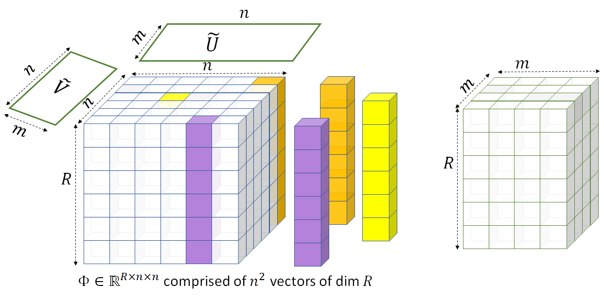
Figure 1: The figure shows the setting of Theorem 2.1 with $d=2$. Left: The linear operator $\Phi:\mathbb{R}^{n\times n}\to\mathbb{R}^{R}$ interpreted as a tensor consisting of a $n\times n$ array of $R$-dimensional vectors. There are smoothed or random contractions applied using matrices $\widetilde{U},\widetilde{V}\in\mathbb{R}^{n\times m}$. Right: The operator $\Phi(\widetilde{U}\otimes\widetilde{V}):\mathbb{R}^{m\times m}\to\mathbb{R}^{R}$ interpreted as an $m^{2}$ array of $R$-dimensional vectors. Theorem 2.1 shows that under the conditions of the theorem, with high probability the robust rank is $m^{2}$.

Informal Theorem 2.1 (Non-symmetric version for $d=2$ and modal contractions).

Suppose $\Phi\in\mathbb{R}^{R\times n^{d}}$ is a matrix with at least $\Omega(n^{2})$ singular values larger than $1$, and let $\widetilde{U},\widetilde{V}$ be random $\rho$-perturbations of arbitrary matrices $U,V$. Then if $m\leq cn$ for an appropriate small constant $c>0$, we have with probability $\geq 1-\exp(-\Omega(n))$ that

$$\sigma_{\min}\Big{(}\Phi(\widetilde{U}\otimes\widetilde{V})\Big{)}\geq\mathrm{poly}\left(\rho,\frac{1}{n}\right).$$

(See Theorem 5.2 for the formal statement for general $d$.)

Smoothed modal contractions

While $\Phi$ is specified as a linear operator or a matrix of dimension $R\times n^{2}$ in Theorem 2.1, one can alternately view $\Phi$ as a order-$3$ tensor of dimensions $R\times n\times n$ as shown in Figure 1. Theorem 2.1 then gives a lower bound for the multilinear rank (or its robust analog) under smoothed modal contractions (dimension reduction) along the modes of dimension $n$ each. The proof of this theorem is by induction on the order $d$. We perform each modal contraction one at a time. As shown in Figure 2, we first do modal contraction by $\widetilde{V}$ to obtain a $R\times n\times m$ tensor $W$ and then by $\widetilde{U}$ to form the final $R\times m\times m$ tensor. We need to argue about the (robust) ranks of the matrix slices (we also call them blocks) and tensors obtained in intermediate steps. For any matrix $M$ (potentially a matrix slice of the tensor $\Phi$) of large (robust) rank $k>1.1m$, a smoothed contraction $M\tilde{U}$ has full rank $m$ (i.e., non-negligible least singular value) with probability $1-\exp(-\Omega(k))$. To argue that the final tensor (when flattened) has full rank $m^{2}$, we need to argue that for the tensor in the intermediate step $W$, each of the $m$ slices (along the contracted mode) has rank at least $\Omega(n)$. The original rank of $\Phi$ was large, so we know that a constant fraction of the slices $\Phi_{1},\dots,\Phi_{n}$ must have rank $\Omega(n)$. But this alone may not be enough since many of the slices can be identical, in which case the $m$ slices are not sufficiently different from each other.

We can use the large rank of $\Phi$ to argue that a constant fraction of the matrix slices should have large “marginal rank” i.e., they have large rank even if we project out the column spaces of the slices that were chosen before it. While this strategy may work in the non-robust setting, this incurs an exponential blowup in the least singular value. Instead we use the following randomized strategy of finding a collection of blocks or slices $S_{1}\subset[n]$, each of which has a large “relative rank”, even after we project out the column spaces of all the other blocks in $S_{1}$ (we show these statements in a robust sense, formalized using appropriate least singular values).

Finding many blocks with large relative rank

We note that while the idea is quite intuitive, the proof of the corresponding claim (Lemma 5.4) is non-trivial because we require that in any selected block, there must be many vectors with a large component orthogonal to the entire span of the other selected blocks. As a simple example, consider setting $n_{2}=2t$ and $\Phi_{1}=\{e_{1},e_{2},\dots,e_{t},\varepsilon e_{t+1},\varepsilon e_{t+2},\dots,\varepsilon e_{2t}\}$, and $\Phi_{2}=\{\varepsilon e_{1},\varepsilon e_{2},\dots,\varepsilon e_{t},e_{t+1},e_{t+2},\dots,e_{2t}\}$. In this case, even if $\varepsilon$ is tiny, we cannot choose both the blocks, because the span of the vectors in $\Phi_{2}$ contains all the vectors in $\Phi_{1}$.

The proof will proceed by first identifying a set of roughly $R=\Omega(n^{2})$ vectors (spread across the blocks) that form a well conditioned matrix, followed by randomly restricting to a subset of the blocks. We start with the following claim, which gives us the first step.

Claim 2.2 (Same as Lemma 5.7).

Suppose $A$ is an $m\times n$ matrix such that $\sigma_{k}(A)\geq\theta$. Then there exists a submatrix $A_{S}$ with $|S|=k$ columns, such that $\sigma_{k}(A_{S})\geq\theta/\sqrt{nk}$.

The lemma is a robust version of the simple statement that if $\sigma_{k}(A)>0$, then there exist $k$ linearly independent columns. The proof of the claim is elegant and uses the choice of a so-called Auerbach basis or a well-conditioned basis for the column span.

The outline of the main argument is as follows:

1. First find a submatrix $M$ of $R=\delta n^{2}$ columns of $\Phi$ such that $\sigma_{R}(M)$ is large

2. Randomly sample a subset $T\subseteq[n]$ of the blocks.

3. Discard any block $j\in T$ that has fewer than $\delta n/6$ vectors with a non-negligible component orthogonal to the span of $\cup_{r\in(T\setminus\{j\})}\Phi_{r}$; argue that there are $\Omega(\delta n)$ blocks remaining.

We remark that the above idea of a random restriction to obtain many blocks with large relative rank (in a robust sense) seems of independent interest and also comes in handy in the application to power sum decompositions (Claim 8.5).

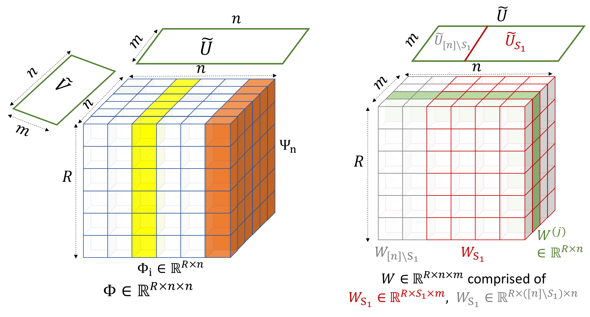
Figure 2: Left: The setting of $d=2$ with linear operator $\Phi:\mathbb{R}^{n\times n}\to\mathbb{R}^{R}$ having slices $\Phi_{1},\dots,\Phi_{n}\in\mathbb{R}^{R\times n}$. The modal contractions $\widetilde{U},\widetilde{V}\in\mathbb{R}^{n\times m}$ have not yet been applied. Right: After modal contraction along $\widetilde{V}\in\mathbb{R}^{n\times m}$, we get $W\in\mathbb{R}^{R\times n\times m}$ with slices $W_{1},\dots,W_{n}$. $W_{S_{1}}\in\mathbb{R}^{R\times S_{1}\times m}$ represents the slices obtained from the “good” blocks $S_{1}\subset[n]$, and $W_{[n]\setminus S_{1}}\in\mathbb{R}^{R\times([n]\setminus S_{1})\times m}$ represents the remaining slices. The random modal contraction $\widetilde{U}$ is also split into $\widetilde{U}_{S_{1}}\in\mathbb{R}^{S_{1}\times m},\widetilde{U}_{[n]\setminus S_{1}}\in\mathbb{R}^{[n]\setminus S_{1}\times m}$.

Finishing the inductive argument

As shown in Figure 2, after modal contraction along $\tilde{V}\in\mathbb{R}^{n\times m}$, we get $W\in\mathbb{R}^{R\times n\times m}$ with slices $W_{1},\dots,W_{n}$.

Now we would like to argue that when we perform a smoothed contraction with $\widetilde{U}$, the contracted slices have large rank, while simultaneously preserving the relative rank across the slices. Let $W_{S_{1}}\in\mathbb{R}^{R\times S_{1}\times m}$ represent the subtensor corresponding to the slices obtained from the “good” blocks $S_{1}\subset[n]$ (which have large relative rank), and let $W_{[n]\setminus S_{1}}\in\mathbb{R}^{R\times([n]\setminus S_{1})\times m}$ represent the remaining slices. Also let $W^{(j)}\in\mathbb{R}^{R\times n}$ denote the matrix slices along the alternate mode for each $j\in[m]$. We can show that the randomly contracted matrices $W^{(j)}_{S_{1}}$ have large relative rank with respect to each other. The random modal contraction $\widetilde{U}$ can also now be split into $\widetilde{U}_{S_{1}}\in\mathbb{R}^{S_{1}\times m},\widetilde{U}_{[n]\setminus S_{1}}\in\mathbb{R}^{[n]\setminus S_{1}\times m}$. The final matrix slice obtained for each $j\in[m^{d-1}]$ can be written as

$$M^{(j)}=W^{(j)}_{S_{1}}\widetilde{U}_{S_{1}}+W^{(j)}_{[n]\setminus S_{1}}\widetilde{U}_{[n]\setminus S_{1}},$$

where the randomness in the two summands is independent. Arguing that the high relative rank across the slices is preserved involves some work, and this is achieved in Lemma 5.5. The lemma proves that with high probability, every test unit vector $\alpha\in\mathbb{R}^{m\cdot m}$ has non-negligible value of $\lVert M\alpha\rVert_{2}$. A standard argument would consider a net over all potential unit vectors $\alpha\in\mathbb{R}^{m\cdot m}$. However this approach fails here, since we cannot get high enough concentration (of the form $e^{-\Omega(m^{2})}$) that is required for this argument. Instead, we argue that if there were such a test vector $\alpha\in\mathbb{R}^{m\cdot m}$, there exists a block $j^{*}\in[m]$ where we get a highly unlikely event. This allows us to conclude the inductive proof that establishes Theorem 2.1.

3 Preliminaries

We now introduce our basic definitions and notation. For a matrix $U\in\mathbb{R}^{n\times m}$, let $\|U\|$ and $\|U\|_{F}$ denote the operator and Frobenius norms of $U$, respectively. Central to the paper are $\rho$-smoothed matrices. In particular, given a matrix $U\in\mathbb{R}^{n\times m}$, we let $\tilde{U}=U+E$ where $E\in\mathcal{N}(0,\rho^{2})$. We commonly call $\tilde{U}$ a $\rho$-smoothing of $U$ or a $\rho$-perturbation of $U$. Similar notation is used for vector inputs $x=(x_{1},\dots,x_{n})$ to a polynomial $p:\mathbb{R}^{n}\to\mathbb{R}^{m}$. I.e., $\tilde{x}=x+\eta$ where $\eta\in\mathcal{N}(0,\rho^{2})$. Thus, for example, $p(\tilde{x})$ is the evaluation of $p$ on a $\rho$-smoothed $x$.

Products.

We also frequently use the Kronecker product, denoted $\otimes$, and the Khatri-Rao product, denoted $\odot$. Given matrices, $A\in\mathbb{R}^{n\times m}$ and $B\in\mathbb{R}^{k\times\ell}$, the Kronecker product $A\otimes B$ is the block matrix

$$A\otimes B=\begin{bmatrix}a_{11}B&\dots&a_{1m_{1}}B\\ \vdots&\ddots&\vdots\\ a_{n_{1}1}B&\dots&a_{n_{1}m_{1}}B\end{bmatrix}\in R^{nk\times m\ell}.$$

We let $A^{\otimes d}\in R^{n^{d}\times m^{d}}$ denote the Kroncker product of a total of $d$ copies of $A$. In the case that $m=\ell$, the Khatri-Rao product $A\odot B$ is defined by

$$A\odot B=\begin{bmatrix}\uparrow&&\uparrow\\ a_{1}\otimes b_{1}&\dots&a_{m}\otimes b_{m}\\ \downarrow&&\downarrow\end{bmatrix}\in\mathbb{R}^{nk\times m}.$$

Here $a_{j}$ and $b_{j}$ denote the $j$th column of $A$ and $B$, respectively, and $a_{j}\otimes b_{j}$ is the Kronecker product (or simply the tensor product) of these columns.

For vector spaces $\mathcal{U},\mathcal{V}$, the tensor product space $\mathcal{U}\otimes\mathcal{V}=\{u\otimes v:u\in\mathcal{U},v\in\mathcal{V}\}$. When $\mathcal{U}=\mathcal{V}$, we also call $\mathcal{U}^{\otimes 2}=\mathcal{U}\otimes\mathcal{U}$ a lift of the space $\mathcal{U}$ (of degree/order $2$). This can also be generalized to $d$-wise products and lifts. When $\mathcal{U}=\mathbb{R}^{n}$, the space $(\mathbb{R}^{n})^{\otimes d}$ corresponds to the space of all $d$-th order tensors of dimensions $n\times n\dots\times n$. This is isomorphic to the space $\mathbb{R}^{n^{d}}$; each tensor can be flattened to form a vector in $n^{d}$ dimensions i.e., $(\mathbb{R}^{n})^{\otimes d}\cong\mathbb{R}^{n^{d}}$.

Symmetrized products.

We are often concerned with symmetrized versions of matrix products. To handle these, we introduce a (partially) symmetrized Kronecker product $\circledast$ which is defined for tuples of matrices $(U^{(1)},\dots,U^{(d)})$ where $U^{(j)}\in\mathbb{R}^{n_{j}\times m}$. We define $U^{(1)}\circledast U^{(2)}\circledast\dots\circledast U^{(d)}\in\mathbb{R}^{\Pi_{i=1}^{d}n_{j}\times\binom{m+d-1}{d}}$ to be the matrix with columns indexed by tuples $(i_{1},i_{2},\dots,i_{d})$ with $1\leq i_{1}\leq i_{2}\leq\dots\leq i_{d}\leq m$ where the column corresponding to $(i_{1},i_{2},\dots,i_{d})$ is

$$\frac{1}{|S_{d}|}\sum_{\pi\in S_{d}}u^{(1)}_{i_{\pi(1)}}\otimes u^{(2)}_{i_{\pi(2)}}\otimes\dots\otimes u^{(d)}_{i_{\pi(d)}}.$$

Here $S_{d}$ denotes the symmetric group on $[d]$ and $u^{(j)}_{i_{\pi(j)}}$ denotes the $i_{\pi(j)}$th column of $U^{(j)}$. For example, for matrices $U,V\in\mathbb{R}^{n\times m}$, the column of $U\circledast V$ corresponding to a tuple $(i,j)$ with $i\leq j$ is

$$\frac{1}{2}(u_{i}\otimes v_{j}+u_{j}\otimes v_{j}).$$

In the case that $i=j$, this reduces to $u_{i}\otimes v_{i}$. For a matrix $U\in\mathbb{R}^{n\times m}$, we let $U^{\circledast d}\in\mathbb{R}^{n^{d}\times\binom{m+d-1}{d}}$ denote the $\circledast$ product of a total of $d$ copies of $U$. The product $\circledast$ can be viewed as a partially symmetrized version of the Kronecker product since all columns of $U^{\circledast d}$ are symmetric with respect to the natural symmetrization of $\mathbb{R}^{n^{d}}\cong(\mathbb{R}^{n})^{\otimes d}$.

Along these lines, we introduce the operator $\mathsf{Sym}_{d}:\mathbb{R}^{n^{d}}\to\mathbb{R}^{n^{d}}$ which symmetrizes elements of $\mathbb{R}^{n^{d}}$ with respect to the identification $\mathbb{R}^{n^{d}}\cong(\mathbb{R}^{n})^{\otimes d}$. With this notation, we have that

$$\mathsf{Sym}_{d}(U^{\circledast d})=U^{\circledast d}.$$

Moreover, the columns of the matrix $U^{\circledast d}$ are precisely the unique columns of the matrix $\mathsf{Sym}_{d}(U^{\otimes d})$.

Finally, for a vector space $\mathcal{U}$, we have that $\mathcal{U}^{\circledast d}=\mathsf{Sym}_{d}(\mathcal{U}^{\otimes d})$ is the space of symmetric $d$th tensors over the spacd $\mathcal{U}$. We also call this the symmetric $d$th order left of the space $\mathcal{U}$.

Leave-one-out distance.

The leave-one-out distance of a matrix $U$ is a useful tool for analyzing least singular values. Given $U\in\mathbb{R}^{n\times m}$, define the leave-one-out distance $\ell(U)$ by

$$\ell(U)=\min_{i}\mathrm{dist}\left(u_{i},\mathrm{Span}\{u_{j}:j\neq i\}\right).$$

The least singular value of $U$ is related to the leave-one-out distance of $U$ through the following lemma [RV08].

Lemma 3.1 (Leave one out distance).

Let $U\in\mathbb{R}^{n\times m}$. Then

$$\frac{\ell(U)}{\sqrt{m}}\leq\sigma_{\min}(U)\leq\ell(U).$$

See also Lemma A.2 for a block-version of leave-one-out singular value bounds.

In our work we also encounter the Jacobian of a polynomial map. Given a vector valued function $P(x)=(p_{1}(x),p_{2}(x),\dots,p_{N}(x))$ over underlying variables $x=(x_{1},x_{2},\dots,x_{n})$, the Jacobian is defined as the $(n\times N)$ matrix of partial derivatives where the $(i,j)$th entry is $\frac{\partial p_{j}}{\partial x_{i}}$. Thus, the linear approximation of $P(x)$ around a point $x$ is simply $P(x+\eta)=P(x)+J(x)^{T}\eta$.

4 Hierarchical Nets and Anti-concentration from Jacobian Conditioning

In this section, we will primarily deal with a matrix $\mathcal{M}$ of dimensions $N\times m$ where $m<N$. The columns will be denoted by $\widetilde{X}_{i}$, and we wish to show a lower bound on $\sigma_{m}(\mathcal{M})$.

In this section, we describe the finer $\varepsilon$-net argument outlined in Section 2. We begin with a formal definition of the CAA property.

Definition 4.1 (CAA property).

We say that a random matrix $\mathcal{M}$ with $m$ columns has the CAA property with parameter $\beta>0$, if ?? for all $k\geq 1$, ?? for all test vectors $\alpha\in\mathbb{R}^{m}$ with at least $k$ coordinates of magnitude $\delta$, there exist $\lambda>0$ and $c\geq\frac{8}{\beta}$ (dependent only on $\mathcal{M}$) such that

$$\forall h\in(0,1),\quad\operatorname*{\mathbb{P}}[\lVert\mathcal{M}\alpha\rVert<\delta h/\lambda]\leq\exp\left(-c\min(m,km^{\beta})\log(1/h)\right).$$

Remark.

We note that the condition $c\geq 8/\beta$ may seem strong; however, as we will see in applications, it is satisfied as long as $m$ is small enough compared to $N$, the number of rows of the matrix.

4.1 Hierarchical nets

The following shows that the CAA property implies a least singular value guarantee.

Theorem 4.2.

Suppose $\mathcal{M}$ is a random matrix with $m$ columns and that $\mathcal{M}$ satisfies the CAA property with some parameter $\beta>0$. Suppose additionally that we have the spectral norm bound $\lVert\mathcal{M}\rVert\leq L$ with probability $1-\eta$. Then with probability at least $1-\exp(-m^{\beta})-\eta$, we have

$$\sigma_{m}(\mathcal{M})\geq\frac{1}{(Lm\lambda)^{2\lceil\frac{1}{\beta}\rceil}},$$

where $\lambda$ comes from the CAA property.

As discussed in Section 2, the natural approach to proving such a result would be to take nets based on the sparsity of the test vector $\alpha$. In other words, if there are $k$ nonzero values of magnitude $\delta>0$, the CAA property yields a least singular value lower bound of $\delta/\lambda$ (choosing $h$ to be a small constant), and we can take a union bound over a net of size $\exp(k)$. The issue with this argument is that $\alpha$ might have many other non-zero values that are slightly smaller than $\delta$, and these might lead to a zero singular value (unless it so happened that $\lambda<1/m$, which we do not have a control of). Of course, in this case, we should have worked with a slightly smaller value of $\delta$, but this issue may recur, so we need a more careful argument.

The rest of this subsection will focus on proving Theorem 4.2. For defining the nets, we will use threshold values $\tau_{1}=1/m$, $\tau_{2}=\theta/m$, and so on (more generally, $\tau_{j}=\theta^{j-1}/m$). $\theta$ is a parameter that will be chosen appropriately; for now we simply use $\theta\in(0,1/m)$.

We construct a sequence of nets $\mathcal{N}_{1},\mathcal{N}_{2},\dots,\mathcal{N}_{s-1}$ as follows. The net $\mathcal{N}_{1}$ is a set of vectors parametrized by pairs $(r_{1},r_{2})\in\mathbb{N}^{2}$, where: (a) $1\leq r_{1}\leq m^{1-\beta}$, (b) $r_{2}\leq m^{\beta}r_{1}$. For each pair $(r_{1},r_{2})$, we include all the vectors whose entries are integer multiples of $\frac{\theta}{m}$ with have exactly $(r_{1}+r_{2})$ non-zero entries, of which $r_{1}$ entries are in $(\tau_{1},1]$ and $r_{2}$ entries are in $[\tau_{2},\tau_{1}]$.

Thus, the number of vectors in $\mathcal{N}_{1}$ for a single pair $(r_{1},r_{2})$ is bounded by:

$$\binom{m}{r_{1}}\binom{m}{r_{2}}\left(\frac{m}{\theta}\right)^{r_{1}}\left(\frac{m}{\theta}\right)^{r_{2}}<\left(\frac{m}{\theta}\right)^{2(r_{1}+r_{2})}.$$

The next net $\mathcal{N}_{2}$ has vectors parametrized by $(r_{1},r_{2},r_{3})\in\mathbb{N}^{3}$, where (a) $r_{2}\leq m^{1-\beta}$, (b) $r_{3}\leq m^{\beta}r_{2}$, and additionally, (c) $r_{2}\geq m^{\beta}r_{1}$. For each such tuple, we include vectors that have exactly $(r_{1}+r_{2}+r_{3})$ non-zero entries (in the corresponding $\tau$ ranges as above), and have values that are all integer multiples of $\theta^{2}/m$.

More generally, the vectors of $\mathcal{N}_{j}$ will be parametrized by $(r_{1},r_{2},\dots,r_{j+1})\in\mathbb{N}^{j+1}$, where (a) $r_{j}\leq m^{1-\beta}$, (b) $r_{j+1}\leq m^{\beta}r_{j}$, and additionally, (c) for $1\leq i<j$, we have $r_{i+1}>m^{\beta}r_{i}$. In other words, $r_{j+1}$ is the first value that does not grow by a factor $m^{\beta}$. For every such tuple, $\mathcal{N}_{j}$ includes all vectors that have exactly $(r_{1}+\dots+r_{j+1})$ non-zero entries, each of which is an integer multiple of $\frac{\theta^{j}}{m}$, and exactly $r_{i}$ of them in the range $(\tau_{i},\tau_{i-1}]$ for all $i\leq j+1$.

We have nets of this form for $j=1,2,\dots,s-1$, where $s=\lceil\frac{1}{\beta}\rceil$. We now have the following claim.

Claim 4.3.

Fix any $1\leq j<s$. We have

$$\operatorname*{\mathbb{P}}\left[\exists\alpha\in\mathcal{N}_{j},\lVert\mathcal{M}\alpha\rVert<\frac{\theta^{j-\frac{1}{2}}}{m\lambda}\right]<\exp\left(-\tfrac{1}{2}cm^{j\beta}\right).$$

Proof.

First consider any single $\alpha\in\mathcal{N}_{j}$. By assumption, it has $r_{j}$ coordinates with magnitude $\geq\frac{\theta^{j-1}}{m}$. Thus, from the CAA property,

$$\operatorname*{\mathbb{P}}\left[\lVert\mathcal{M}\alpha\rVert<\frac{\theta^{j-1}}{m}\frac{h}{\lambda}\right]\leq\exp\left(-cr_{j}m^{\beta}\log(1/h)\right).$$ (2)

The number of vectors in $\mathcal{N}_{j}$ for a given tuple of $r_{j}$ values is clearly bounded by $\left(\frac{m}{\theta^{j}}\right)^{r_{1}+r_{2}+\dots+r_{j+1}}$. We choose $h=\theta^{1/2}$, and $\theta<1/m$, and argue that as long as these are true,

$$(r_{1}+\dots+r_{j+1})\log\frac{m}{\theta^{j}}\leq\frac{c}{2}r_{j}m^{\beta}\log(1/h).$$ (3)

We can simplify this by noting that from our assumptions on $r_{j}$, $r_{j}m^{\beta}\geq\frac{1}{2}(r_{1}+r_{2}+\dots+r_{j+1})$. Thus to show (3), it suffices to have

$$\frac{c}{4}\log\frac{1}{h}\geq\log\frac{m}{\theta^{j}}.$$

Since $\theta<1/m$, we have $\theta^{j}/m>\theta^{j+1}>\theta^{s}$. Since $c\geq 8s$ and $h=\theta^{1/2}$, the above inequality holds, and so inequality (3) also holds.

Next, we observe that for any tuple of $\{r_{i}\}$ values in $\mathcal{N}_{j}$, since $r_{1}\geq 1$, we have $r_{j}\geq m^{(j-1)\beta}$, which implies that $r_{j}m^{\beta}\geq m^{j\beta}$. Using this fact, together with (3), we first take a union bound over all $\alpha\in\mathcal{N}_{j}$ corresponding to a given tuple $(r_{i})_{1\leq i\leq j+1}$ (call this set $\mathcal{N}_{j}^{\prime}$ for now), and obtain

$$\operatorname*{\mathbb{P}}\left[\exists\alpha\in\mathcal{N}_{j}^{\prime}:\lVert\mathcal{M}\alpha\rVert<\frac{\theta^{j-\frac{1}{2}}}{m\lambda}\right]<\exp\left(-\frac{c}{2}m^{j\beta}\log(1/h)\right).$$

Now since the total number of tuples is easily bounded by $m^{j+1}\leq m^{s}$, taking a further union bound over these choices and simplifying, we obtain the claim. ∎

Finally, we have a bigger net for all “dense” vectors $\alpha$, that have at least $m^{1-\beta}$ coordinates of magnitude $\geq\frac{\theta^{s-1}}{m}$. This net consists of vectors $\in\mathbb{R}^{m}$ for which (a) every coordinate is an integer multiple of $\theta^{s}/m$ (between $0$ and $1$), and (b) at least $m^{1-\beta}$ coordinates are $\geq\frac{\theta^{s-1}}{m}$. Call this net $\mathcal{N}_{0}$.

An easy upper bound for the size is

$$|\mathcal{N}_{0}|\leq\left(\frac{m}{\theta^{s}}\right)^{m}.$$

Using this, we have the following:

Claim 4.4.

$$\operatorname*{\mathbb{P}}\left[\exists\alpha\in\mathcal{N}_{0}:\lVert\mathcal{M}\alpha\rVert<\frac{\theta^{s-\frac{1}{2}}}{m\lambda}\right]<\exp\left(-\frac{c}{2}m\right).$$

Proof.

First, consider any fixed $\alpha\in\mathcal{N}_{0}$. Using part (b) of the definition of $\mathcal{N}_{0}$, we can use the CAA property to obtain

$$\operatorname*{\mathbb{P}}\left[\lVert\mathcal{M}\alpha\rVert<\frac{\theta^{s-1}h}{m\lambda}\right]<\exp\left(-cm\log(1/h)\right),$$

for any parameter $h$. As before, we show that this is small enough to take a union bound over $|\mathcal{N}_{0}|$ terms. Specifically, we argue that setting $h=\theta^{1/2}$,

$$\log|\mathcal{N}_{0}|\leq m\log\frac{m}{\theta^{s}}\leq\frac{1}{4}cm\log\frac{1}{\theta}.$$

The latter holds because $\theta<1/m$, and $c\geq 8s\geq 4(s+1)$. This completes the proof. ∎

We can now complete the proof of Theorem 4.2 as follows.

Proof of Theorem 4.2..

Consider any $\alpha\in\mathbb{R}^{m}$ with $\lVert\alpha\rVert=1$. Also, suppose we condition on the event that $\lVert\mathcal{M}\rVert\leq L$ (which happens with probability $1-\eta$). Let $s=\lceil\frac{1}{\beta}\rceil$ as before. Now define $r_{1},r_{2},\dots r_{s}$ to be the number of entries of $\alpha$ in the intervals $(\frac{1}{m},1],(\frac{\theta}{m},\frac{1}{m}]$, and so on. We consider two cases:

Case 1. $(r_{1}+r_{2}+\dots+r_{s})\geq m^{1-\beta}$. I.e., there are sufficiently many “large” coordinates in $\alpha$.

In this case, we observe that there exists a vector $\alpha^{\prime}\in\mathcal{N}_{0}$ such that $\lVert\alpha-\alpha^{\prime}\rVert\leq\theta^{s}$. Now, we have from Claim 4.4 that with high probability, $\lVert\mathcal{M}\alpha^{\prime}\rVert\geq\frac{\theta^{s-\frac{1}{2}}}{m\lambda}$. If this holds, then $\lVert\mathcal{M}\alpha\rVert\geq\frac{\theta^{s-\frac{1}{2}}}{m\lambda}-L\theta^{s}$, where $L$ is the spectral norm bound on $\mathcal{M}$. We choose $\theta$ such that

$$L\theta^{1/2}<\frac{1}{m\lambda}\iff\theta<\frac{1}{m^{2}L^{2}\lambda^{2}}.$$

Thus for this value of $\theta$,

$$\operatorname*{\mathbb{P}}\left[\exists\alpha,\lVert\alpha\rVert=1,\text{ satisfying (Case 1)}:~{}\lVert\mathcal{M}\alpha\rVert<\frac{\theta^{s-\frac{1}{2}}}{2m\lambda}\right]<\exp\left(-\frac{c}{2}m\right).$$ (4)

Case 2. $(r_{1}+r_{2}+\dots+r_{s})<m^{1-\beta}$. In this case, we claim that we must have some index $j<s$ such that $r_{j+1}/r_{j}\leq m^{\beta}$. This is because $r_{1}\geq 1$ (a unit vector must have some entry $>1/m$), and if the above does not hold, then $r_{j}>m^{(j-1)\beta}$. Plugging $j=s$ gives a contradiction to our assumption that $(r_{1}+r_{2}+\dots r_{s})<m^{1-\beta}$.

Thus, let $j$ be the smallest index for which we have $r_{j+1}/r_{j}\leq m^{\beta}$. We can now consider the net $\mathcal{N}_{j}$ and find some $\alpha^{\prime}\in\mathcal{N}_{j}$ such that $\lVert\alpha-\alpha^{\prime}\rVert<\theta^{j}$.

We can use an argument identical to the one in (Case 1), this time leveraging Claim 4.3, to conclude that for all $j$,

$$\operatorname*{\mathbb{P}}\left[\exists\alpha,\lVert\alpha\rVert=1,\text{satisfying (Case 2)}:\lVert\mathcal{M}\alpha\rVert<\frac{\theta^{s-\frac{1}{2}}}{2m\lambda}\right]<\sum_{1\leq j<s}\exp\left(-\frac{c}{2}m^{j\beta}\right).$$

The first term on the RHS dominates, and plugging in the chosen values of $\theta,s$, this completes the proof. ∎

One of the advantages of our $\varepsilon$-net argument is that if we only care about “well spread” vectors, we can obtain a much stronger concentration bound (Eq (4)).

Observation 4.5.

Suppose $\mathcal{M}$ is a random matrix that satisfies the CAA property with parameter $\beta$. Let us call a test vector $\alpha$ (of length $\leq 1$) “dense” if it has at least $m^{1-\beta}$ coordinates of magnitude $>\delta$. Then

$$\operatorname*{\mathbb{P}}\left[\exists\text{ dense }\alpha:\lVert\mathcal{M}\alpha\rVert<\frac{1}{(Lm\lambda)^{2\lceil\frac{1}{\beta}\rceil}}\right]<\exp\left(-\tfrac{1}{2}cm\right).$$

Note that in the above claim, $m$ could be quite large compared to $n$. The observation follows immediately from (4), but we will use it later in Section 6.3.

5 Higher Order Lifts of Smoothed Matrices

We provide the following theorem.

Theorem 5.1.

Suppose $d\in\mathbb{N}$, and let $\Phi:\mathsf{Sym}^{d}(\mathbb{R}^{n})\to\mathbb{R}^{D}$ be an orthogonal projection of rank $R=\delta\binom{n+d-1}{d}$ for some constant $\delta>0$, and let $\mathsf{Sym}_{d}:(\mathbb{R}^{n})^{\otimes d}\to\mathsf{Sym}^{d}(\mathbb{R}^{n})$ be the orthogonal projection on to the symmetric subspace of $(\mathbb{R}^{n})^{\otimes d}$. Let $U=(u_{i}:i\in[m])\in\mathbb{R}^{n\times m}$ be an arbitrary matrix, and let $\tilde{U}$ be a random $\rho$-perturbation of $U$. Then there exists a constant $c_{d}>0$ such that for $m\leq c_{d}\delta n$, with probability at least $1-\exp\big{(}-\Omega_{d,\delta}(n)\big{)}$, we have the least singular value

$$\sigma_{\binom{m+d-1}{d}}(\Phi\tilde{U}^{\circledast d}) \geq\frac{\rho^{d}}{n^{O(d)}},\text{ where }$$

$$\tilde{U}^{\circledast d} \coloneqq\Big{(}\mathsf{Sym}_{d}(\tilde{u}_{i_{1}}\otimes\tilde{u}_{i_{2}}\dots\otimes\tilde{u}_{i_{d}}):1\leq i_{1}\leq i_{2}\leq\dots\leq i_{d}\leq n\Big{)}.$$ (5)

In the above statement, one can also consider an arbitrary linear operator $\Phi$ and suffer an extra factor of $\sigma_{R}(\Phi)$ in the least singular value bound (by considering the projector onto the span of the top $R$ singular vectors). In the rest of the section, we assume that $\Phi$ is an orthogonal projector of rank $R$ without loss of generality.

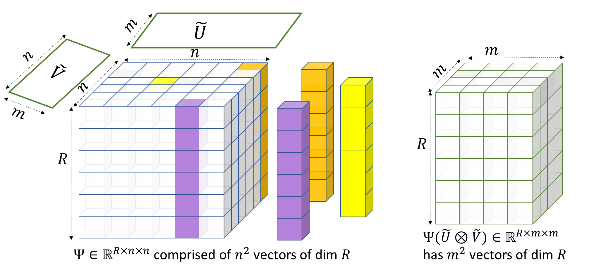
Figure 3: Left: The linear operator $\Psi:\mathbb{R}^{n\times n}\to\mathbb{R}^{R}$ interpreted as a tensor consisting of a $n\times n$ array of $R$-dimensional vectors. There are smoothed or random contractions applied using matrices $\tilde{U},\tilde{V}\in\mathbb{R}^{n\times m}$. Right: The operator $\Psi(\tilde{U}\otimes\tilde{V}):\mathbb{R}^{m\times m}\to\mathbb{R}^{R}$ interpreted as an $m^{2}$ array of $R$-dimensional vectors. Theorem 5.2 shows that under the conditions of the theorem, with high probability the robust rank of this operator is $m^{2}$ i.e, the least singular value of $R\times m^{2}$ matrix is inverse polynomial.

Theorem 5.1 follows from the following theorem (Theorem 5.2) which gives a non-symmetric analog of the same statement. The proof of Theorem 5.1 follows from a reduction to Theorem 5.2 that is given by Lemma 5.9. In what follows, $\Psi\in\mathbb{R}^{R\times n^{d}}$ denotes the natural matrix representation of $\Phi$ such that $\Psi x^{\otimes d}=\Phi(x^{\otimes d})$ for all $x\in\mathbb{R}^{n}$.

Theorem 5.2.

Suppose $\ell\in\mathbb{N}$, $R=\delta\binom{n+d-1}{d}$ for some constant $\delta>0$ and let $\Psi:(\mathbb{R}^{n})^{\otimes\ell}\to\mathbb{R}^{D}$ be a linear operator with $\sigma_{R}(\Psi)\geq 1$. Suppose random matrices $\tilde{U}^{(1)},\dots,\tilde{U}^{(d)}\in\mathbb{R}^{n\times m}$ are generated as follows:

$$\forall j\in[d],\ \tilde{U}^{(j)}=U^{(j)}+Z^{(j)},\text{ where }Z^{(j)}\sim_{i.i.d}\mathcal{N}(0,\rho^{2})^{n\times m}\text{ and is independent of }U^{(j)},$$

while $U^{(j)}\in\mathbb{R}^{n\times m}$ is arbitrary and can also depend on $\tilde{U}^{(j+1)},\dots,\tilde{U}^{(d)}$. Then there exists constants $c_{d},c^{\prime}_{d}>0$ and an absolute constant $c_{0}\geq 1$ such that for $m\leq c_{d}\delta n$, with probability at least $1-\exp\big{(}-\Omega_{d,\delta}(n)\big{)}$, we have

$$\sigma_{m^{d}}\Big{(}\Psi\big{(}\tilde{U}^{(1)}\otimes\dots\otimes\tilde{U}^{(d)}\big{)}\Big{)} \geq\frac{c^{\prime}_{d}\rho^{d}}{n^{c_{0}d}}.$$ (6)

While $\Psi$ is specified as a matrix of dimension $R\times n^{d}$ in Theorem 5.2, one can alternately view $\Psi$ as a $(d+1)$-order tensor of dimensions $R\times n\times n\times\dots\times n$ as shown in Figure 3. Theorem 5.2 then gives a lower bound for the multilinear rank (in fact, for its robust analog) under smoothed modal contractions along the $d$ modes of dimension $n$ each.

Applying Theorem 5.1 along with the block leave-one-out approach (see Lemma A.2) we arrive at the following corollary.

Corollary 5.3.

Suppose $d,t\in\mathbb{N}$ and let $1\geq\delta_{1}>\delta_{2}>0$ be given. Also let $\Phi:\mathsf{Sym}^{d}(\mathbb{R}^{n})\to\mathbb{R}^{D}$ be an orthogonal projection of rank $R\geq\delta_{1}\binom{n+d-1}{d}$. Let $\{U_{j}\}_{j=1}^{t}\subset\mathbb{R}^{n\times m}$ be an arbitrary collection of $n\times m$ matrices, and for each $j$, let $\tilde{U}_{j}$ be a random $\rho$-perturbation of $U_{j}$. Then there exists a constant $c_{d}>0$ such that if $t\binom{m+d-1}{d}\leq\delta_{2}\binom{n+d-1}{d}$ and $m\leq c_{d}(\delta_{1}-\delta_{2})n$, then with probability at least $1-\exp\big{(}-\Omega_{d,\delta_{1},\delta_{2}}(n)\big{)}$, we have the least singular value

$$\sigma_{t\binom{m+d-1}{d}}\left(\Phi\begin{bmatrix}\tilde{U}_{1}^{\circledast d}&\tilde{U}_{2}^{\circledast d}&\dots&\tilde{U}_{t}^{\circledast d}\end{bmatrix}\right) \geq\frac{\rho^{d}}{\sqrt{t}n^{O(d)}}.$$ (7)

Proof.

For each $j=1,\dots,t$, let $\Pi_{-j}$ denote the orthgonal projection onto

$$\mathrm{range}(\Phi)\cap\Big{(}\mathrm{range}\big{(}[\tilde{U}_{1}^{\circledast d}\ \dots\tilde{U}_{j-1}^{\circledast d}\ \tilde{U}_{j+1}^{\circledast d}\ \dots\tilde{U}_{t}^{\circledast d}]\big{)}\Big{)}^{\perp}.$$

We first lower bound the least singular value of $\Pi_{-j}(\tilde{U}_{j}^{\circledast d}).$ Observe that from our assumptions, the rank of $\Pi_{-j}$ is at least

$$\delta_{1}\binom{n+d-1}{d}+(1-\delta_{2})\binom{n+d-1}{d}-\binom{n+d-1}{d}=(\delta_{1}-\delta_{2})\binom{n+d-1}{d}.$$

Taking $c_{d}$ to be the constant from Theorem 5.1, we can then apply Theorem 5.1 to conclude that with probability at least $1-\exp(-\Omega_{d,\delta_{1},\delta_{2}}(n))$ we have

$$\sigma_{\binom{m+d-1}{d}}(\Pi_{-j}\tilde{U}_{j}^{\otimes d})\geq\frac{\rho^{d}}{n^{O(d)}}.$$

The result now follows by applying the block leave one out bound of Lemma A.2. ∎

5.1 Proof of Theorem 5.2

We will prove Theorem 5.2 for general $d$ by induction on $d$. The following crucial lemma considers a linear operator $\Psi$ acting on the space $\mathbb{R}^{n_{1}}\otimes\mathbb{R}^{n_{2}}$, and shows that if $\Psi$ has large rank $\Omega(n_{1}n_{2})$, then it has many “blocks” of large relative rank as described in Section 2.3.

Lemma 5.4.

Let $\Psi\in\mathbb{R}^{R\times(n_{1}n_{2})}$ be a projection matrix of rank $R=\delta n_{1}n_{2}$ for some constant $\delta>0$, and let $\Psi=[\Psi_{1}\ \Psi_{2}\ \dots\ \Psi_{n_{1}}]$ where the blocks $\Psi_{i}\in\mathbb{R}^{R\times n_{2}}~{}\forall i\in[n_{1}]$. Then there exists constants $c_{1},c_{2},c_{3}>0$ and a subset $S_{1}\subset[n_{1}]$ with $|S_{1}|\geq c_{1}\delta n_{1}$ such that

$$\forall i\in S_{1},~{}\sigma_{c_{2}\delta n_{2}}\Big{(}\Pi^{\perp}_{S_{1}\setminus\{i\}}\Psi_{i}\Big{)}\geq\frac{1}{(nk)^{c_{3}}},$$ (8)

where $\Pi^{\perp}_{S}$ is the projection orthogonal to $\mathrm{span}\big{(}\cup_{i\in S}\mathrm{colspan}(\Psi_{i})\big{)}$.

We prove this lemma in Section 5.2 by restricting to randomly chosen columns as described in the overview (Section 2.3). We now proceed with the proof of Theorem 5.2 assuming the above lemma.

The following lemma will be important in the inductive proof of the theorem. It reasons about the robust rank (also called multi-linear rank) after the modal contraction by a smoothed matrix along a specific mode. The lemma is proved in slightly more generality; we will use it for the theorem with $\varepsilon=1$.

Lemma 5.5 (Robust rank under random contractions).

Suppose $\varepsilon\in(0,1]$ is a constant. For every constant $\gamma,C>0$, there is a constant $c\in(0,1)$ such that the following holds for all $s=2^{o(k)}$. Consider matrices $A_{1},A_{2},\dots,A_{s}\in\mathbb{R}^{R\times k}$, $C_{1},\dots,C_{s}\in\mathbb{R}^{R\times m}$ and $\forall j\in[s]$ let $\Pi^{\perp}_{-j}$ denote the projector orthogonal to the span of the column spaces of $\{A_{j^{\prime}}:j^{\prime}\neq j,j^{\prime}\in[s]\}$. Suppose the following conditions are satisfied:

$$\forall j\in[s],~{}\sigma_{\varepsilon k}(\Pi^{\perp}_{-j}A_{j})\geq k^{-\gamma}$$ (9)

and $\sigma_{1}(A_{j}),\sigma_{1}(C_{j})\leq k^{C}$. For a random $\rho$-perturbed matrix $\tilde{U}\in\mathbb{R}^{k\times m}$ with $m\leq c\varepsilon k$, we have with probability at least $1-\exp(-\Omega(\varepsilon k))$ that

$$\text{if }~{}\forall j\in[s],~{}M_{j}=C_{j}+A_{j}\tilde{U},\text{ then }\sigma_{sm}\Big{(}M_{1}\mid M_{2}\mid\dots\mid M_{s}\Big{)}\geq\frac{\rho}{2k^{\gamma+1}\sqrt{s}}.$$

Proof.

Let $\tilde{U}=U+Z$ where $Z\sim N(0,\rho^{2})^{k\times m}$ is the random perturbation. Denote $M=(M_{1}\mid\dots\mid M_{s})$. Recall $\Pi^{\perp}_{-j^{*}}$ is the projector orthogonal to the span of the column spaces of $\{A_{j}:j\neq j^{*},j\in[s]\}$. We prove that with high probability, for any (test) unit vector $\alpha\in\mathbb{R}^{s\cdot m}$, we have $\lVert M\alpha\rVert_{2}$ is non-negligible. A standard argument would consider a net over all potential unit vectors $\alpha\in\mathbb{R}^{sm}$. However this approach fails here, since we cannot get high enough concentration (of the form $e^{-\Omega(sm)}$) that is required for this argument. Instead, we argue that if there were such a test vector $\alpha\in\mathbb{R}^{s\cdot m}$, there exists a block $j^{*}\in[s]$ where we observe a highly unlikely event.

We will use the following simple claim that is proven using a standard net argument.

Claim 5.6.

In the above notation, given a (fixed) vector $w\in\mathbb{R}^{R}$, and a random matrix $Z\sim N(0,\rho^{2})^{R\times k}$ with i.i.d entries, we have that with probability at least $1-\exp(-\Omega(k))$ that

$$\forall v\in\mathbb{R}^{m}\text{ with }\lVert v\rVert_{2}=1\text{ and }\forall j\in[s],~{}\lVert w+\Pi^{\perp}_{-j}(A_{j}Z)v\rVert_{2}\geq\frac{\rho}{2k^{\gamma+1}}$$

Proof of Claim. We first prove the claim using a net argument over test vectors $v\in\mathbb{R}^{m}$. Consider a fixed $j\in[s]$; we will do a union bound over all $j\in[s]$.

Let $v\in\mathbb{R}^{m}$ be a fixed unit vector. Let $A^{\prime}=\Pi^{\perp}_{-j}A_{j}$. Observe that $Zv\sim N(0,\rho^{2}I)$ is a random Gaussian vector with i.i.d entries each with mean $0$ and variance $1$. By assumption $\sigma_{\varepsilon k}(A^{\prime})=\sigma_{\varepsilon k}(\Pi^{\perp}_{-j}A_{j})\geq k^{-\gamma}$. Let the SVD of $A^{\prime}=E\text{diag}(\mu)F^{\top}=\sum_{i=1}^{k}\mu_{i}e_{i}f_{i}^{\top}$ where $\mu_{i}\geq 0~{}\forall i\in[k]$ and $\mu_{1}\geq\mu_{2}\geq\dots\geq\mu_{\varepsilon k}\geq k^{-\gamma}$.

$$A^{\prime}(Zv)=E\text{diag}(\mu)(FZv)=E\text{diag}(\mu)\zeta=\sum_{i=1}^{k}\zeta_{i}\mu_{i}e_{i},$$

where $\zeta\sim N(0,I)$ is a random Gaussian vector with i.i.d entries. Moreover $\mu_{i}\geq k^{-\gamma}$ for all $i\in[\varepsilon k]$. Hence $\forall\delta\in(0,1/2)$,

$$\operatorname*{\mathbb{P}}\Big{[}\lVert w+\Pi^{\perp}_{-j}A_{j}Zv\rVert<\frac{\delta\rho}{k^{\gamma}}\Big{]} \leq\operatorname*{\mathbb{P}}\Big{[}\forall i\in[\varepsilon k],|\langle w,e_{i}\rangle+\langle e_{i},\Pi^{\perp}_{-j}A_{j}Zv\rangle|<\frac{\delta\rho}{k^{\gamma}}\Big{]}$$

$$=\prod_{i=1}^{\varepsilon k}\operatorname*{\mathbb{P}}\Big{[}|\langle w,e_{i}\rangle+\mu_{i}\zeta_{i}|<\frac{\delta\rho}{k^{\gamma}}\Big{]}\leq(c_{0}\delta)^{\varepsilon k},$$

for some absolute constant $c_{0}>0$. The equality used the independence of $(\zeta_{i}:i\in[k])$, while the last inequality used that $\mu_{i}\geq k^{-\gamma}$ for $i\leq\varepsilon k$ along with standard anti-concentration of a Gaussian r.v.

Set $\varepsilon^{\prime}\coloneqq\delta/(4k^{C+1/2})$. Consider an $\varepsilon^{\prime}$-net $\mathcal{N}_{\varepsilon^{\prime}}$ over unit vectors in $\mathbb{R}^{m}$. By a union bound over $\mathcal{N}_{\varepsilon^{\prime}}$, we get

$$\operatorname*{\mathbb{P}}\Big{[}\forall j\in[s],\forall\hat{v}\in\mathcal{N}_{\varepsilon},\lVert w+\Pi^{\perp}_{-j}A_{j}Z\hat{v}\rVert\geq\frac{\delta\rho}{k^{\gamma}}~{}\Big{]} \geq 1-s(c\delta)^{\varepsilon k}|\mathcal{N}_{\varepsilon^{\prime}}|$$

$$\geq 1-\exp\Big{(}-\varepsilon k\log\big{(}\tfrac{1}{c\delta}\big{)}+\log s+m\log(2/\varepsilon^{\prime})\Big{)}$$

$$\geq 1-\exp(-\Omega(k)),$$

by picking $\delta=1/k$, and $m\leq c\varepsilon k$ for an appropriately small constant $c>0$ (depending on $C$). Finally conditioned on the above event, for any unit vector $v\in\mathbb{R}^{k}$, we can consider the closest point $\hat{v}$ in $\mathcal{N}_{\varepsilon^{\prime}}$ and conclude that $\forall j\in[s],\lVert\Pi^{\perp}_{-j}A_{j}Zv\rVert\geq\lVert\Pi^{\perp}_{-j}A_{j}Zv\rVert-\lVert A_{j}\rVert\lVert Z\rVert\lVert v-\hat{v}\rVert\leq O(k^{C}\cdot\sqrt{k}\rho)\varepsilon^{\prime}\geq\frac{\delta\rho}{2k^{\gamma}}$.

Finishing the proof of Lemma 5.5 Let us condition on the event that the conclusion of Claim 5.6 holds; note that this holds with probability at least $1-\exp(-\Omega(\varepsilon k))$.

Suppose for contradiction there exists a vector $\alpha\in\mathbb{R}^{s\cdot k}$ such that $\lVert M\alpha\rVert_{2}<\frac{\rho}{k^{\gamma+1}\sqrt{s}}$. The vector $M\alpha\in\mathbb{R}^{R}$ is

$$M\alpha =\sum_{j\in[s]}M_{j}\alpha^{(j)}=\sum_{j\in[s]}\big{(}C_{j}+A_{j}(U+Z)\big{)}\alpha^{(j)}=\sum_{j\in[s]}\big{(}C_{j}+A_{j}U\big{)}\alpha^{(j)}+\sum_{j\in[s]}A_{j}Z\alpha^{(j)}$$

$$=b_{\alpha}+\sum_{j\in[s]}A_{j}Z\alpha^{(j)},$$ (10)

where $b_{\alpha}$ is a fixed vector in $\mathbb{R}^{R}$. We have for all $j^{*}\in[s]$

$$\Pi^{\perp}_{-j^{*}}M\alpha =\Pi^{\perp}_{-j^{*}}b_{\alpha}+\sum_{j\in[s]}\Pi^{\perp}_{-j^{*}}A_{j}Z\alpha^{(j)}$$

$$=\Pi^{\perp}_{-j^{*}}b_{\alpha}+\Pi^{\perp}_{-j^{*}}A_{j^{*}}(Z\alpha^{(j^{*})}),$$ (11)

In the above, (11) holds since $\Pi^{\perp}_{-j^{*}}$ is orthogonal to the column spaces of all $j\neq j^{*}$ and $A^{\prime}=\Pi^{\perp}_{-j^{*}}A_{j^{*}}$.

Now consider any index $j^{*}\in[s]$ such that $\lVert\alpha^{(j^{*})}\rVert_{2}\geq 1/\sqrt{s}$ (note $\sum_{j=1}^{s}\lVert\alpha^{(j)}\rVert^{2}_{2}=1$). Now applying Claim 5.6 with $j=j^{*}$, $v=\alpha^{(j^{*})}/\lVert\alpha^{(j^{*})}\rVert$ and $w=\Pi^{\perp}_{-j^{*}}b_{\alpha}/\lVert\alpha^{(j^{*})}\rVert$, we get that

$$\lVert M\alpha\rVert_{2}\geq\lVert\Pi^{\perp}_{-j^{*}}M\alpha\rVert\geq\frac{1}{\sqrt{s}}\cdot\frac{\rho}{2k^{\gamma+1}},$$

which contradicts the assumption. This concludes the proof.

∎

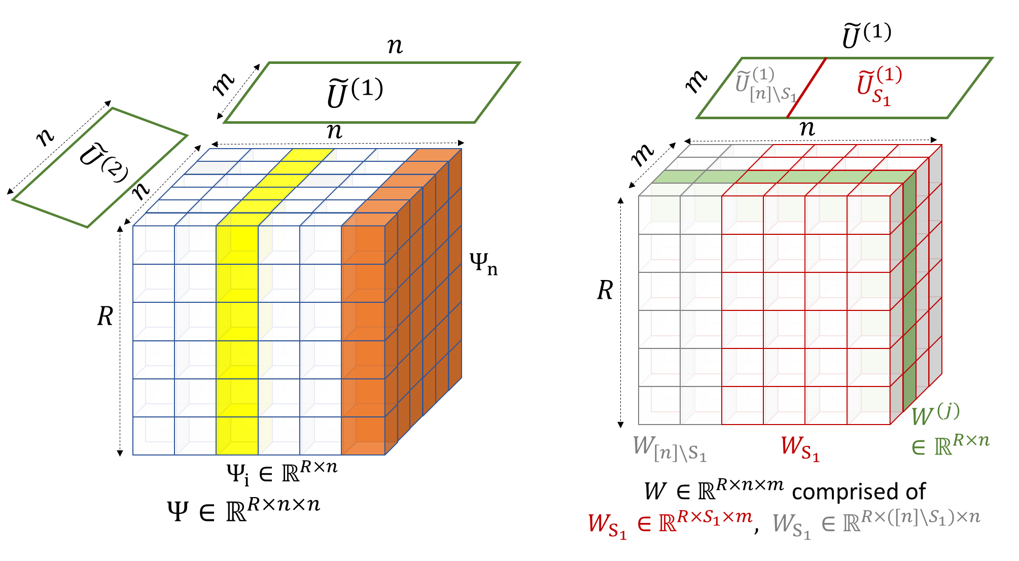
Figure 4: Left: The setting of $d=2$ with linear operator $\Psi:\mathbb{R}^{n\times n}\to\mathbb{R}^{R}$ having slices $\Psi_{1},\dots,\Psi_{n}\in\mathbb{R}^{R\times n}$. The modal contractions $\tilde{U}^{(1)},\tilde{U}^{(2)}\in\mathbb{R}^{n\times m}$ have not yet been applied. Right: After modal contraction along $U^{(2)}\in\mathbb{R}^{n\times m}$, we get $W\in\mathbb{R}^{R\times n\times m}$ with lateral slices $W_{1},\dots,W_{n}$. The subtensor $W_{S_{1}}\in\mathbb{R}^{R\times|S_{1}|\times m}$ represents the slices obtained from the “good” blocks $S_{1}\subset[n]$, and $W_{[n]\setminus S_{1}}\in\mathbb{R}^{R\times|[n]\setminus S_{1}|\times m}$ represents the remaining slices. The random modal contraction $\tilde{U}^{(1)}$ can also now be split into $\tilde{U}^{(1)}_{S_{1}}\in\mathbb{R}^{S_{1}\times m},\tilde{U}^{(1)}_{[n]\setminus S_{1}}\in\mathbb{R}^{[n]\setminus S_{1}\times m}$. Let $W^{(j)}\in\mathbb{R}^{R\times n}$ denote the $j$th frontal slice for each $j\in[m^{d-1}]$. Then the final matrix slice obtained for each $j\in[m^{d-1}]$ can be written as $M^{(j)}=W^{(j)}_{S_{1}}\tilde{U}^{(1)}_{S_{1}}+W^{(j)}_{[n]\setminus S_{1}}\tilde{U}^{(1)}_{[n]\setminus S_{1}}$, where the randomness in the two summands is independent.

Proof of Theorem 5.2.

We now proceed by induction on $d$. For the proof it will be useful to think of $\rho$ as a sufficiently small inverse polynomial (this is without loss of generality and suffers only a $\mathrm{poly}(n)$ extra factor in the bound).

The base case $d=1$ follows by simple random matrix arguments; specifically, Lemma 5.5 applied with $s=1,d=1$ implies it.

For higher $d$, we will apply the induction hypothesis for modal contractions along the last $d-1$ modes using matrices $\tilde{U}^{(2)},\dots,\tilde{U}^{(d)}$, and then finally apply modal contraction along $\tilde{U}^{(1)}$.

Set $n_{1}=n,n_{2}=n^{d-1}$. First applying Lemma 5.4 with $\Psi$ (i.e., applied with the projection matrix onto the top $R$ singular vectors), we get a set of blocks $\{\Psi_{i}:i\in S_{1}\}$ with $|S_{1}|=\Omega(\delta n_{1})$, satisfying (8). Define for each $i\in S_{1}$, $\mathcal{V}_{i}\coloneqq\mathrm{colspan}(\Psi_{i})$, and $\mathcal{V}_{-i}\coloneqq\mathrm{span}(\cup_{j\in S_{1},j\neq i}\mathrm{colspan}(\Psi_{i}))$ and let $\Pi^{\perp}_{-i}$ be the projection matrix for the subspace orthogonal to $\mathcal{V}_{-i}$. Then for absolute constants $c,c^{\prime}>0,c^{\prime\prime}>0$,

$$\sigma_{c\delta n^{d-1}}\Big{(}\Pi^{\perp}_{-i}\Psi_{i}\Big{)}\geq\frac{c^{\prime\prime}}{(nk)^{c^{\prime}}}\text{ for all }i\in S_{1}.$$

Also suppose for each $i\in[n]$ that $W_{i}\coloneqq\Psi_{i}\big{(}\tilde{U}^{(2)}\otimes\tilde{U}^{(3)}\otimes\dots\otimes\tilde{U}^{(d)}\big{)}\in\mathbb{R}^{R\times m^{d-1}}$. By using the induction hypothesis with order $(d-1)$ with the matrices $\{\Pi^{\perp}_{-i}\Psi_{i}\}$ along with a union bound over the $n$ blocks, for appropriate constants $c_{0}>0$ and $c^{\prime}_{d-1}>0$,

$$\forall i\in S_{1},~{}\sigma_{m^{d-1}}\Big{(}\Pi^{\perp}_{-i}W_{i}\Big{)}=\sigma_{m^{d-1}}\Big{(}\Pi^{\perp}_{-i}\Psi_{i}\big{(}\tilde{U}^{(2)}\otimes\dots\otimes\tilde{U}^{(d)}\big{)}\Big{)}\geq\frac{c^{\prime}_{d-1}\rho^{d-1}}{n^{c_{0}(d-1)}}.$$ (12)

Let $W\in\mathbb{R}^{R\times n\times m^{d-1}}$ be the tensor obtained by stacking the matrices $W_{i}\in\mathbb{R}^{R\times m^{d-1}}$ as shown in the Figure 4. Let $W_{S_{1}}\in\mathbb{R}^{R\times S_{1}\times m^{d-1}}$ denote the subtensor comprising just the slices $i\in S_{1}$, and let $W_{[n]\setminus S_{1}}$ be the remaining portion. For each $j\in[m^{d-1}]$, let $W^{(j)}\in\mathbb{R}^{R\times n}$ be obtained from the slices along the third mode. We will use $W^{(j)}_{S_{1}},W^{(j)}_{[n]\setminus S_{1}}$ to denote the portions of the slices $W^{(j)}$ formed by the columns $S_{1}$ and $[n]\setminus S_{1}$ respectively. If $W^{\textrm{flat}}_{S_{1}}\in\mathbb{R}^{R\times(|S_{1}|m^{d-1})}$ is the matrix obtained by flattening $W_{S_{1}}$ appropriately, then by Lemma A.2 on the block leave-one-out distance,

$$\sigma_{|S_{1}|m^{d-1}}\Big{(}W^{\textrm{flat}}_{S_{1}}\Big{)}=\sigma_{|S_{1}|m^{d-1}}\Big{(}W_{S_{1}}^{(1)}\mid\dots\mid W_{S_{1}}^{(m^{d-1})}\Big{)}\geq\frac{c^{\prime}_{d-1}\rho^{d-1}}{n^{c_{0}(d-1)+\tfrac{1}{2}}}.$$ (13)

The final matrix is obtained by concatenating the matrices $M^{(j)}\in\mathbb{R}^{R\times m}$ for each $j\in[m^{d-1}]$, where

$$M^{(j)} =W^{(j)}\tilde{U}^{(1)}=W^{(j)}_{S_{1}}\tilde{U}^{(1)}_{S_{1}}+W^{(j)}_{[n]\setminus S_{1}}\tilde{U}^{(1)}_{[n]\setminus S_{1}}$$

$$=W^{(j)}_{S_{1}}\tilde{U}^{(1)}_{S_{1}}+C^{(j)},~{}\text{ where }C^{(j)}\coloneqq W^{(j)}_{[n]\setminus S_{1}}\tilde{U}^{(1)}_{[n]\setminus S_{1}}.$$

Consider any fixed $j\in[m^{d-1}]$. We will treat $C^{(j)}$ as fixed matrices. Note that the randomness in $\tilde{U}^{(1)}_{S_{1}}$ is independent of the randomness in $\tilde{U}^{(1)}_{[n]\setminus S_{1}}$. Now we can apply Lemma 5.5 with $s=m^{d-1}$, $A_{j}=W^{(j)}_{S_{1}}$ and $\tilde{U}=\tilde{U}^{(1)}_{S_{1}}$ and $C_{j}=C^{(j)}$ to conclude the inductive proof of Theorem 5.2. ∎

5.2 Finding many blocks with large relative rank

We note that while the statement of the lemma is quite intuitive, the proof is non-trivial because we require that in any selected block, there must be many vectors with a large component orthogonal to the entire span of the other selected blocks. As a simple example, consider setting $n_{2}=2t$ and $\Psi_{1}=\{e_{1},e_{2},\dots,e_{t},\varepsilon e_{t+1},\varepsilon e_{t+2},\dots,\varepsilon e_{2t}\}$, and $\Psi_{2}=\{\varepsilon e_{1},\varepsilon e_{2},\dots,\varepsilon e_{t},e_{t+1},e_{t+2},\dots,e_{2t}\}$. In this case, even if $\varepsilon$ is tiny, we cannot choose both the blocks, because the span of the vectors in $\Psi_{2}$ contains all the vectors in $\Psi_{1}$.

The proof will proceed by first identifying a set of roughly $R$ vectors (spread across the blocks) that form a well conditioned matrix, followed by randomly restricting to a subset of the blocks.

We start with the following lemma, which gives us the first step.

Lemma 5.7.

Suppose $A$ is an $m\times n$ matrix such that $\sigma_{k}(A)\geq\theta$. Then there exists a submatrix $A_{S}$ with $|S|=k$ columns, such that $\sigma_{k}(A_{S})\geq\theta/\sqrt{nk}$.

Remark.

The lemma is a robust version of the simple statement that if $\sigma_{k}(A)>0$, then there exist $k$ linearly independent columns.

Proof.

We start by noting that we can restrict to the case $m=k$. This is because we can project the columns of $A$ onto the span of the top $k$ singular vectors of $A$ and pick the $S$ using the resulting matrix. Formally, if $\Pi$ is the $(k\times m)$ matrix that defines the projection, then we work with $\Pi A$. (By definition, $\sigma_{k}(\Pi A)=\sigma_{k}(A)\geq\theta$, so the hypothesis of the lemma holds.) For the obtained set $S$, it is easy to see that the vectors before projection will satisfy, for any test vector $\alpha$,

$$\|\sum_{i}\alpha_{i}v_{i}\|\geq\|\sum_{i}\alpha_{i}\Pi v_{i}\|.$$

Thus if we show a lower bound for $\sigma_{k}(\Pi A_{S})$, the same bound holds for $\sigma_{k}(A_{S})$. So in what follows, assume that $m=k$.

Next, we find an Auerbach basis [LT13] (also referred to as a Barycentric spanner or a well-conditioned basis [AK08, HK16]) for the columns of $A$. Recall that this is a subset of the columns of $A$ defined by a subset $S$ of indices such that $|S|=k$, and for all $i\in[n]$, $A_{i}$ can be expressed as $\sum_{j\in S}\alpha_{j}A_{j}$ with $|\alpha_{j}|\leq 1$.

We claim that for this choice of $S$, we have a lower bound on $\sigma_{k}(A_{S})$. Suppose not; suppose $\|\sum_{i\in S}\alpha_{i}A_{i}\|<\theta/\sqrt{nk}$ for some unit vector $\alpha$ (whose non-zero entries are indexed by $S$). Since $\alpha$ is a unit vector with at most $k$ non-zeros, one of its coefficients, say $\alpha_{j}$, must be $\geq 1/\sqrt{k}$. Thus we have $A_{j}=x+w$, for some $x\in\text{span}(A_{S\setminus\{j\}})$ and $\|w\|\leq\theta/\sqrt{n}$.

Next, consider any column $A_{\ell}$ for $\ell\not\in S$. From the above, we have that $A_{\ell}$’s projection orthogonal to the span of $A_{S\setminus\{j\}}$ is at most $\theta/\sqrt{n}$ (because of the Auerbach basis property, and the fact that $A_{j}$ is almost in the span of $A_{S\setminus\{j\}}$). This implies that the squared rank-$(k-1)$ approximation error (in the Frobenius norm) of the matrix $A$ is $\leq(n-k)\theta^{2}/n<\theta^{2}$, which contradicts the fact that $\sigma_{k}(A)\geq\theta$. ∎

We can now complete the proof of Lemma 5.4.

Proof of Lemma 5.4.

The outline of the argument is as follows:

1. First find a subset $M$ of $R=\delta n_{1}n_{2}$ columns of $\Psi$ such that $\sigma_{R}(M)$ is large (using Lemma 5.7).

2. Randomly sample a subset $T\subseteq[n_{1}]$ of the blocks.

3. Discard any block $j\in T$ that has fewer than $\delta n_{2}/6$ vectors with a non-negligible component orthogonal to the span of $\cup_{r\in(T\setminus\{j\})}\Psi_{r}$; argue that there are $\Omega(\delta n_{1})$ blocks remaining.

The first step is a direct application of Lemma 5.7; we thus obtain $M$ with $R=\delta n_{1}n_{2}$ columns such that

$$\sigma_{R}(M)\geq\frac{1}{n_{1}n_{2}\sqrt{\delta}}.$$ (14)

For convenience, we will denote the columns of $M$ by $v_{1},v_{2},\dots,v_{R}$.

Now for the second step of the outline: $T\subseteq[n_{1}]$ is selected by including each block $j$ in $T$ with probability equal to $|M\cap\Psi_{j}|/6n_{2}$. I.e., the probability is proportional to the fraction of the “$M$” columns contained in a block. For convenience, we will write $\alpha_{j}=|M\cap\Psi_{j}|/n_{2}$.

Step (3) of the outline is thus the bulk of the argument. We start by introducing two random variables. First, for $j\in[n_{1}]$, define $X_{j}$ to be the indicator that is $1$ if block $j$ is chosen in $T$ and $0$ otherwise. Thus by definition, $\operatorname*{\mathbb{P}}[X_{j}=1]=\alpha_{j}/6$, and the $X_{j}$ are independent for different $j$. Second, for $i\in[R]$, if $j$ is the index of the block that contains $v_{i}$, we define $Y_{i}$ to be $1$ if the vector $v_{i}$ has a projection of length $\geq\frac{1}{Rn_{1}n_{2}\sqrt{\delta}}$ orthogonal to the span of all the columns in $\cup_{r\in T\setminus\{j\}}\Psi_{r}$ and $0$ otherwise.

Now, note that a block $j$ “survives” step (3) of the outline above if (a) $j\in T$ to start with, and (b) $\sum_{v_{i}\in\Psi_{j}}Y_{i}\geq\delta n_{2}/6$. [This is a sufficient condition for survival, not an equivalence.] Thus, if $Q_{j}$ is a random variable indicating if block $j$ survives, we can write

$$Q_{j}\geq\frac{X_{j}\left(\sum_{v_{i}\in\Psi_{j}}Y_{i}-\frac{\delta n_{2}}{6}\right)_{+}}{n_{2}\alpha_{j}}.$$ (15)

Here, for a random variable $Z$, the notation $(Z)_{+}$ denotes $\max\{Z,0\}$. We will use the RHS expression to give a positive lower bound on $\operatorname*{\mathbb{E}}[\sum_{j\in[n_{1}]}Q_{j}]$. Note that this will complete the proof of the lemma, because we are only interested in an existential statement.

To this end, the key observation is that for any $v_{i}\in\Psi_{j}$, the random variable $Y_{i}$ is independent of $X_{j}$. This is because by definition, $Y_{i}$ indicates if $v_{i}$ had a large enough component orthogonal to the span of the other chosen blocks (irrespective of whether block $j$ is chosen or not). Thus, since $\operatorname*{\mathbb{E}}[X_{j}]=\alpha_{j}/6$, we have that

$$\operatorname*{\mathbb{E}}\left[\frac{X_{j}\left(\sum_{v_{i}\in\Psi_{j}}Y_{i}-\frac{\delta n_{2}}{6}\right)_{+}}{n_{2}\alpha_{j}}\right]=\frac{1}{6n_{2}}\operatorname*{\mathbb{E}}\left[\left(\sum_{v_{i}\in\Psi_{j}}Y_{i}-\frac{\delta n_{2}}{6}\right)_{+}\right]\geq\frac{1}{6n_{2}}\left(\operatorname*{\mathbb{E}}[\sum_{v_{i}\in\Psi_{j}}Y_{i}]-\frac{\delta n_{2}}{6}\right).$$

Thus, we have

$$\sum_{j\in[n_{1}]}Q_{j}\geq\frac{1}{6n_{2}}\left(\operatorname*{\mathbb{E}}\big{[}\sum_{i\in[R]}Y_{i}\big{]}-\frac{\delta n_{1}n_{2}}{6}\right).$$ (16)

So it complete the proof, it suffices to prove that $\mathbb{E}[\sum_{i}Y_{i}]$ is sufficiently large. We do this by introducing an auxiliary random variable $Z_{i}$. For any $i\in[R]$, define $Z_{i}$ to be the random variable that is $1$ if $v_{i}$ has a projection of length $\geq\frac{1}{Rn_{1}n_{2}\sqrt{\delta}}$ orthogonal to the span of the vectors in all the chosen blocks, $\cup_{r\in T}\Psi_{r}$.

Thus by definition, the inequality $Z_{i}\leq Y_{i}$ always holds, and $Z_{i}$ will be zero if $X_{j}=1$ (where $\Psi_{j}$ is the block that contains $v_{i}$). We will prove that in fact, $\operatorname*{\mathbb{E}}[\sum_{i}Z_{i}]$ is large. Observe that by the law of conditional expectation,

$$\operatorname*{\mathbb{E}}[\sum_{i}Z_{i}]=\sum_{T}\operatorname*{\mathbb{P}}[T]\cdot\operatorname*{\mathbb{E}}[\sum_{i}Z_{i}|T].$$

Indeed, the last term is deterministic conditioned on $T$ (so it is simply the number of $i$ for which $Z_{i}$ is 1 for the chosen $T$). We split the sum into two, depending on $|T|$.

$$\operatorname*{\mathbb{E}}[\sum_{i}Z_{i}]=\sum_{T:|T|>2n_{1}\delta/3}\operatorname*{\mathbb{P}}[T]\cdot\operatorname*{\mathbb{E}}[\sum_{i}Z_{i}|T]+\sum_{T:|T|\leq 2n_{1}\delta/3}\operatorname*{\mathbb{P}}[T]\cdot\operatorname*{\mathbb{E}}[\sum_{i}Z_{i}|T].$$

We will simply ignore the first sum, as our goal is to obtain a lower bound. To show that this is good enough, we first observe that

$$\operatorname*{\mathbb{E}}[|T|]=\sum_{j\in[n_{1}]}X_{j}=\sum_{j}\frac{\alpha_{j}}{6}\leq\frac{\delta n_{1}}{6}.$$

Thus by Markov’s inequality, $\operatorname*{\mathbb{P}}[|T|\leq 2n_{1}\delta/3]\geq 3/4$. Let us thus condition on one such $T$.

Claim. For any $T$ with $|T|\leq 2\delta n_{1}/3$, we have $\sum_{i\in[R]}Z_{i}\geq\frac{\delta n_{1}n_{2}}{3}$.

Informally, $v_{i}$ are vectors that are all “well conditioned”, and thus many of them must have a component orthogonal to any subspace of dimension $<R/2$.

This can be made formal as follows: let $\mathcal{S}$ be the subspace $\mathrm{span}\left(\cup_{r\in T}\Psi_{r}\right)$. Clearly, its dimension is $\leq|T|n_{2}\leq\delta 2n_{1}n_{2}/3=2R/3$. Now from our definition of $\{v_{i}\}$, the matrix $M$ whose columns are the $v_{i}$ has $\sigma_{R}(M)$ bounded as in (14). Thus, if $\Pi_{\mathcal{S}}^{\perp}$ is the matrix that projects every vector to the space $\mathcal{S}^{\perp}$, we have, by the Min-Max characterization of eigenvalues,

$$\sigma_{R-\text{dim}(\mathcal{S})}(\Pi_{\mathcal{S}}^{\perp}M)\geq\sigma_{R}(M)\geq\frac{1}{n_{1}n_{2}\sqrt{\delta}}.$$

Thus, at least $R-\text{dim}(\mathcal{S})\geq\delta n_{1}n_{2}/2$ columns of $\Pi_{\mathcal{S}}^{\perp}M$ must have length $\geq\frac{1}{Rn_{1}n_{2}\sqrt{\delta}}$.

This will let us conclude that $\mathbf{E}[\sum_{i}Z_{i}]\geq\delta n_{1}n_{2}/3$, thus completing the proof of the claim.

Next, we use the claim together with our observations above to conclude that

$$\operatorname*{\mathbb{E}}\left[\sum_{i}Z_{i}\right]\geq\frac{\delta n_{1}n_{2}}{3}\cdot\operatorname*{\mathbb{P}}\left[|T|\leq 2n_{1}\delta/3\right]\geq\frac{\delta n_{1}n_{2}}{3}\cdot\frac{3}{4}=\frac{\delta n_{1}n_{2}}{4}.$$

Plugging this into (16), we obtain $\sum_{j\in[n_{1}]}Q_{j}\geq\Omega(n_{1})$, thus completing the proof. ∎

5.3 From Symmetric to Non-Symmetric Products

Recall $U\in\mathbb{R}^{n\times m}$ and $\tilde{U}=U+Z$ where $U=(u_{i}:i\in[m])$ is an arbitrary matrix and $Z\in\mathbb{R}^{n\times m}$ is a random matrix with i.i.d. entries drawn from $\mathcal{N}(0,\rho^{2})$. In what follows, $\Phi:\mathsf{Sym}(\mathbb{R}^{n^{d}})\to\mathbb{R}^{r}$ denotes an operator acting on the symmetric space, and let $\Psi\in\mathbb{R}^{r\times n^{d}}$ denote the natural matrix representation of $\Phi$ such that $\Phi(x^{\otimes d})=\Psi x^{\otimes d}$, and where where every row of $\Psi$ corresponds to a symmetric matrix.

Additionally, we define $\mathrm{Perm}_{\text{avg}}\in\mathbb{R}^{m^{d}\times\binom{m+d-1}{d}}$ to be the unique matrix with the property that for any collection of matrices $\{V^{(i)}\}_{i=1}^{d}\subset\mathbb{R}^{n\times m}$, we have that $\left(\otimes_{i=1}^{d}V^{(i)}\right)\mathrm{Perm}_{\text{avg}}\in\mathbb{R}^{n^{d}\times\binom{m+d-1}{d}}$ is the matrix with columns indexed by tuples $(i_{1},i_{2},\dots,i_{d})$ with $1\leq i_{1}\leq i_{2}\leq\dots\leq i_{d}\leq m$, where the column corresponding to $(i_{1},i_{2},\dots,i_{d})$ is given by $\frac{1}{|S_{d}|}\left(\sum_{\pi\in S_{d}}\otimes_{j=1}^{d}V^{(j)}_{i_{\pi(j)}}\right)$. Here $S_{d}$ denotes the permutation group on $d$ indices and $V^{(j)}_{i_{\pi(j)}}$ is the $i_{\pi(j)}$th column of $V^{(j)}$.

The matrix $\mathrm{Perm}_{\text{avg}}$ has two important properties that we note. First, for any matrix $U$, we have that $(U^{\otimes d})\mathrm{Perm}_{\text{avg}}$ is the matrix with columns $\mathsf{Sym}_{d}(\tilde{u}_{i_{1}}\otimes\tilde{u}_{i_{2}}\otimes\dots\otimes u_{i_{d}})$ where $1\leq i_{1}\leq i_{2}\dots\leq i_{d}\leq m$. That is $(U^{\otimes d})\mathrm{Perm}_{\text{avg}}=U^{\circledast d}$. It follows that

$$\Big{(}\Phi\big{(}\mathsf{Sym}_{d}~{}\tilde{u}_{i_{1}}\otimes\tilde{u}_{i_{2}}\otimes\dots\otimes u_{i_{d}}\big{)}:1\leq i_{1}\leq i_{2}\dots\leq i_{d}\leq m\Big{)}=\Psi\left(U^{\otimes d}\right)\mathrm{Perm}_{\text{avg}}.$$

Second, since $\Psi$ is determined by ts action on $\mathsf{Sym}(\mathbb{R}^{\otimes d})$, we obtain that for any collection of matrices $\{V^{(i)}\}_{i=1}^{d}\subset\mathbb{R}^{n\times m}$ and any permutation $\pi\in S_{d}$, one has

$$\Psi\left(\otimes_{i=1}^{d}V^{(i)}\right)\mathrm{Perm}_{\text{avg}}=\Psi\left(\otimes_{i=1}^{d}V^{(\pi(i))}\right)\mathrm{Perm}_{\text{avg}}.$$ (17)

The following lemma is useful in our reduction from nonsymmetric products to symmetric products.

Lemma 5.8.

Given $d\in\mathbb{N}$, for each $i=1,\dots,d$, let $Z_{j}\sim\mathcal{N}(0,\rho_{j}^{2})^{n\times m}$ and set $\rho^{2}=\rho_{1}^{2}+\dots+\rho_{d}^{2}$ so that $Z:=Z_{1}+\dots+Z_{d}\sim\mathcal{N}(0,\rho^{2})^{n\times m}$. Also let $\tilde{U}=U+Z\in\mathbb{R}^{n\times m}$ be a $\rho$-smoothed matrix. For each $\ell\in[d]$, set $\tilde{V}^{(\ell)}=\tilde{U}-Z_{1}-\dots-Z_{\ell}$. Then one has

$$\Psi\left(\tilde{U}^{\otimes d}\right)\mathrm{Perm}_{\text{avg}}=\Psi\left(\otimes_{j=1}^{d}(\tilde{V}^{(j)}+(d-j+1)Z_{j})\right)\mathrm{Perm}_{\text{avg}}+\Psi E$$

where the error matrix $E$ is a random matrix that satisfies $\lVert E\rVert_{F}\leq c_{d}(1+\|U\|^{d-2})\rho^{2}(nm)^{\frac{d}{2}})$ with probability at least $1-\exp(-\Omega(nm))$, for some constant $c_{d}>0$ that only depends on $d$.

Proof.

The proof follows an induction argument that carefully leverages symmetry (equation (17)), and groups together terms in a way that decouples the randomness.

We give the proof by induction on $k$. In particular, we will show that for $k\leq d$, we have

$$\Psi\left(\tilde{U}^{\otimes d}\right)\mathrm{Perm}_{\text{avg}}=\Psi\left(\otimes_{j=1}^{k}(\tilde{V}^{(j)}+(d-j+1)Z_{j})\otimes(\tilde{V}^{(k)})^{\otimes d-k}\right)\mathrm{Perm}_{\text{avg}}+\Psi\left(\sum_{j=1}^{k}E_{j}\right)$$

where for each $j$ we have $\lVert E_{j}\rVert_{F}\leq c_{d}^{\prime}O((1+\|U\|^{d-2})\rho_{j}^{2}(nm)^{\frac{d}{2}})$ with probability at least $1-\exp(-\Omega(nm))$ for some constant $c_{d}^{\prime}$ that depends only on $d$. Setting $\tilde{V}^{(0)}:=\tilde{U}$, the statement trivially holds in the base case of $k=0$. We now suppose the result is true for $k=\ell$ and prove it true for $\ell+1$. Set

$$W_{\ell}:=\otimes_{j=1}^{\ell}(\tilde{V}^{(j)}+(d-j+1)Z_{j}).$$

Then using our induction hypothesis with the identity $\tilde{V}^{(\ell)}=\tilde{V}^{(\ell+1)}+Z_{\ell+1}$, we obtain

$$\Psi\left(\tilde{U}^{\otimes d}\right)\mathrm{Perm}_{\text{avg}} =\Psi\left(W_{\ell}\otimes(\tilde{V}^{(\ell)})^{\otimes d-\ell}\right)\mathrm{Perm}_{\text{avg}}+\Psi\left(\sum_{j=1}^{\ell}E_{j}\right)$$

$$=\Psi\left(W_{\ell}\otimes(\tilde{V}^{(\ell+1)}+Z_{\ell+1})^{\otimes d-\ell}\right)\mathrm{Perm}_{\text{avg}}+\Psi\left(\sum_{j=1}^{\ell}E_{j}\right)$$

Applying equation (17) and expanding with the binomial theorem gives

$$\Psi\left(W_{\ell}\otimes\left(\tilde{V}^{(\ell+1)}+Z_{\ell+1})\right)^{\otimes d-\ell}\right)\mathrm{Perm}_{\text{avg}}$$

$$= \Psi\Big{(}W_{\ell}\otimes\Big{(}\sum_{j=0}^{d-\ell}\binom{d-\ell}{j}\left(Z_{\ell+1}^{\otimes j}\right)\otimes\left((\tilde{V}^{(\ell+1)})^{\otimes d-\ell-j}\right)\Big{)}\Big{)}\mathrm{Perm}_{\text{avg}}$$

$$= \Psi\left(W_{\ell}\otimes\bigg{(}\left(\tilde{V}^{(\ell+1)}\right)^{\otimes d-\ell}+(d-\ell)\left(Z_{\ell+1}\right)\otimes\left(\tilde{V}^{(\ell)}\right)^{\otimes d-\ell+1}+E_{\ell+1}^{\prime}\bigg{)}\right)\mathrm{Perm}_{\text{avg}}$$

$$= \Psi\left(W_{\ell}\otimes\left(\tilde{V}^{(\ell+1)}+(d-\ell)Z_{\ell+1}\right)\right)\otimes\left((\tilde{V}^{(\ell+1)})^{\otimes d-\ell-1}\right)\mathrm{Perm}_{\text{avg}}+\Psi(W_{\ell}\otimes E_{\ell+1}^{\prime})\mathrm{Perm}_{\text{avg}}$$

Here

$$E_{\ell+1}^{\prime}:=\sum_{j=2}^{d-\ell}\binom{d-\ell}{j}Z_{\ell+1}^{\otimes j}\otimes(V^{(\ell+1)})^{\otimes d-j}.$$

Setting $E_{\ell+1}:=(W_{\ell}\otimes E_{\ell+1}^{\prime})\mathrm{Perm}_{\text{avg}}$, we obtain that $\lVert E_{\ell+1}\rVert_{F}\leq c_{d}^{\prime}O((1+\|U\|^{d-2})\rho_{j}^{2}(nm)^{\frac{d}{2}})$ with probability at least $1-\exp(-\Omega(nm))$. From here, observing that

$$W_{\ell+1}=W_{\ell}\otimes\left(\tilde{V}^{(\ell+1)}+(d-\ell)Z_{\ell+1}\right)$$

completes the proof by induction. ∎

Lemma 5.9 (Symmetric to Non-symmetric Products).

Suppose $d\in\mathbb{Z}_{+}$ be a positive integer. Suppose $\Phi:\mathsf{Sym}(\mathbb{R}^{n^{d}})\to\mathbb{R}^{r}$ with $\lVert\Phi\rVert\leq 1$. For every $\rho_{1},\dots,\rho_{d}>0$ with $\sum_{j=1}^{d}\rho_{j}^{2}=\rho^{2}$ and $\delta\in(0,1)$ the following holds when $\tilde{U}=U+Z$ is drawn as described above with the entries of $Z$ being drawn i.i.d from $\mathcal{N}(0,\rho^{2})$:

$$\forall t\geq 0,~{} \operatorname*{\mathbb{P}}\Big{[}\sigma_{\binom{m+d-1}{d}}\Big{(}\Phi\big{(}\mathsf{Sym}_{d}\tilde{u}_{i_{1}}\otimes\tilde{u}_{i_{2}}\otimes\dots\otimes u_{i_{d}}\big{)}:1\leq i_{1}\leq i_{2}\dots\leq i_{d}\leq m\Big{)}\leq t\Big{]}$$

$$\leq\operatorname*{\mathbb{P}}\Big{[}\sigma_{m^{d}}\Big{(}\Psi\left(\otimes_{j=1}^{d}(\tilde{V}^{(j)}+(d-j+1)Z_{j})\right)\Big{)}\leq\sqrt{d!}\cdot t+\|E\|\log(1/\delta)\Big{]}+\delta.$$ (18)

Here $V^{(\ell)}=\tilde{U}-Z_{1}-\dots-Z_{\ell}$ and for each $\ell\in[d]$ and $Z_{\ell}$ is a random matrix with i.i.d entries drawn from $\mathcal{N}(0,\rho_{\ell}^{2})$ and $E$ is the error matrix appearing in Lemma 5.8 which has norm $\|E\|=O((1+\|U\|^{d-2})\rho^{2}(n+m)^{\frac{d}{2}})$.

Proof.

First observe that

$$\Phi\big{(}\mathsf{Sym}_{d}\tilde{u}_{i_{1}}\otimes\tilde{u}_{i_{2}}\otimes\dots\otimes u_{i_{d}}\big{)}:1\leq i_{1}\leq i_{2}\dots\leq i_{d}\leq m\Big{)}=\Psi\left(\tilde{U}^{\otimes d}\right)\mathrm{Perm}_{\text{avg}}$$

Using Lemma 5.8 shows then shows that

$$\Psi\left(\tilde{U}^{\otimes d}\right)\mathrm{Perm}_{\text{avg}}=\Psi\left(\otimes_{j=1}^{d}(\tilde{V}^{(j)}+(d-j+1)Z_{j})\right)\mathrm{Perm}_{\text{avg}}+\Psi E.$$

Using the fact that $\mathrm{Perm}_{\text{avg}}$ has columns with disjoint support each with $\ell_{2}$ norm at least $\frac{1}{\sqrt{d!}}$ shows that the matrix $\mathrm{Perm}_{\text{avg}}$ has full column rank with all singular values in $[\frac{1}{\sqrt{d!}},1]$. Combining this with the above equality gives

$$\sigma_{\binom{m+d-1}{d}}\left(\Psi\left(\tilde{U}^{\otimes d}\right)\mathrm{Perm}_{\text{avg}}\right)\geq\frac{1}{\sqrt{d!}}\sigma_{m^{d}}\left(\Psi\left(\otimes_{j=1}^{d}(\tilde{V}^{(j-1)}+jZ_{j})\right)\right)-\|\Psi\|\|E\|,$$

from which the desired singular value lower bound follows. ∎

6 Anticoncentration of a vector of homogeneous polynomials

6.1 Overview

Formally, we consider the following setting: let $p_{1},p_{2},\dots,p_{N}$ be a collection of homogeneous polynomials over $n$ variables $(x_{1},x_{2},\dots,x_{n})$, and define

$$P(x)=\begin{bmatrix}p_{1}(x)\\ p_{2}(x)\\ \vdots\\ p_{N}(x)\end{bmatrix}$$ (19)

Our goal will be to show anticoncentration results for $P$. Specifically, we want to prove that $\operatorname*{\mathbb{P}}[\lVert P(\tilde{x})-y\rVert<\varepsilon]$ is small for all $y$, where $\tilde{x}$ is a perturbation of some (arbitrary) vector $x\in\mathbb{R}^{n}$.

We first observe that such a statement is not hard to prove if we know that the Jacobian $J(x)$ of $P(x)$ has many large singular values at every $x$, and if the perturbation $\rho$ is small enough. This is because around the given point $x$, we can consider the linear approximation of $P(\tilde{x})$ given by the Jacobian. Now as long as the perturbation has a high enough projection onto the span of the corresponding singular vectors of $J(x)$, $P(\tilde{x})$ can be shown to have desired anticoncentration properties (by using the standard anticoncentration result for Gaussians). Finally, if $J(x)$ has $k$ large singular values, a random $\rho$-perturbation will have a large enough projection to the span of the singular vectors with probability $1-\exp(-k)$.

Now, in the applications we are interested in, the polynomials $P$ tend to have the Jacobian property above for “typical” points $x$, but not all $x$. Our main result here is to show that this property suffices. Specifically, suppose we know that for every $x$, the Jacobian at a $\rho$ perturbed point has $k$ singular values of magnitude $\geq c\rho$ with high probability. Then, in order to show anticoncentration, we view the $\rho$ perturbation of $x$ as occurring in two independent steps: first perturb by $\rho\sqrt{1-z^{2}}$ for some parameter $z$, and then perturb by $\rho z$. The key observation is that for Gaussian perturbations, this is identical to a $\rho$ perturbation!

This gives an approach for proving anticoncentration. We use the fact that the first perturbation yields a point with sufficiently many large Jacobian singular values with high probability, and combine this with our earlier result (discussed above) to show that if $z$ is small enough, the linear approximation can indeed be used for the second perturbation, and this yields the desired anticoncentration bound.

Applications. The simplest application for our framework is the setting where $\mathcal{M}$ has columns being $\tilde{u}_{i}\otimes\tilde{v}_{i}$, for some $\rho$-perturbations of underlying vectors $u_{i},v_{i}$. (This setting was studied in [BCMV14, ADM⁺18] and already had applications to parameter recovery in statistical models.) Here, we can show that $\mathcal{M}$ has the CAA property. To show this, we consider some combination $\sum_{i}\alpha_{i}(\tilde{u}_{i}\otimes\tilde{v}_{i})$ with $k$ “large” coefficients in $\alpha$, and show that in this case, the Jacobian property holds. Specifically, we show that the Jacobian has $\Omega(kn)$ large singular values. This establishes the CAA property, which in turn implies a lower bound on $\sigma_{\min}(\mathcal{M})$. This gives an alternative proof of the results of the works above.

6.2 Jacobian rank property and anticoncentration results

We give a sufficient condition for proving such a result, in terms of the Jacobian of $P$. (See Section 3 for background.)

Definition 6.1 (Jacobian rank property).

We say that $P$ has the Jacobian rank property with parameters $(k,c,\gamma)$ if for all $\rho>0$ and for all $x$, the matrix $J(\tilde{x})$ has at least $k$ singular values of magnitude $\geq c\rho$, with probability at least $1-\gamma$. Here, $\tilde{x}=x+\eta$, where $\eta\sim\mathcal{N}(0,\rho^{2})$ is a perturbation of the vector $x$.

Comment.

Indeed, all of our results will hold if we only have the required condition for small enough perturbations $\rho$. To keep the results simple, we work with the stronger definition.

For many interesting settings of $P$, the Jacobian rank property turns out to be quite simple to prove. Our main result now is that the property above implies an anticoncentration bound for $P$.

Theorem 6.2.

Suppose $P(x)$ defined as above satisfies the Jacobian rank property with parameters $(k,c,\gamma)$, and suppose further that the the Jacobian $P^{\prime}$ is $M$-Lipschitz in our domain of interest. Let $x$ be any point and let $\tilde{x}$ be a $\rho$-perturbation. Then for any $h>0$, we have

$$\forall y\in\mathbb{R}^{N},\ \operatorname*{\mathbb{P}}\left[\lVert P(\tilde{x})-y\rVert<\frac{c\rho^{2}h}{64Mnk}\right]\leq\gamma+\exp(-\frac{1}{4}\cdot k\log(1/h)).$$

A key ingredient in the proof is the following “linearization” based lemma.

Lemma 6.3.

Suppose $x$ is a point at which the Jacobian $J(x)$ of a polynomial map $P$ has at least $k$ singular values of magnitude $\geq\tau$. Also suppose that the norm of the Hessian of each $p_{i}(x)$ is bounded by $M$ in the domain of interest. Then, for “small” perturbations, $0<\rho<\frac{\tau}{4Mnk}$, we have that for any $\varepsilon>0$,

$$\forall y,~{}\operatorname*{\mathbb{P}}[\lVert P(\tilde{x})-y\rVert<\varepsilon]<\left(\frac{2\varepsilon}{\tau\rho}\right)^{k}+\left(\frac{2M\rho nk}{\tau}\right)^{k/2}.$$

We remark that the lemma does not imply Theorem 6.2 directly because it only applies to the case where the perturbation $\rho$ is much smaller than the singular value threshold $\tau$.

Proof.

Let $\eta$ be the random perturbation of $x$ as in the lemma statement. We have

$$P(x+\eta)=P(x)+J(x)^{T}\eta+E(\eta),$$

where $E(\eta)$ is an error term, bounded in magnitude by $M\lVert\eta\rVert^{2}$ because of our assumption of the Jacobian being Lipschitz. Now, the desired probability is equivalent to

$$\operatorname*{\mathbb{P}}\left[J(x)^{T}\eta+E(\eta)\in\text{Ball}(y-P(x),\varepsilon)\right].$$

From the bound on $\eta$, the above probability can be upper bounded by

$$\operatorname*{\mathbb{P}}\left[J(x)^{T}\eta\in\text{Ball}\left(y-P(x),\varepsilon+M\lVert\eta\rVert^{2}\right)\right].$$

Let us denote the event in the parentheses above by $\mathcal{E}$. Now, consider the top $k$ singular directions of $J(x)$; suppose the eigenvalues are $\sigma_{1},\sigma_{2},\dots,\sigma_{k}$, and suppose $\eta_{1},\eta_{2},\dots,\eta_{k}$ are the components of $\eta$ along these directions. By hypothesis, $\sigma_{i}\geq\tau$ for all $i\leq k$. Thus if $\mathcal{E}$ occurs, we also have,

$$\forall i\leq k,~{}\sigma_{i}\eta_{i}\in\text{Ball}\left((y-P(x))_{i},\varepsilon+M\lVert\eta\rVert^{2}\right).$$ (20)

Let $\theta>1$ be a parameter that we set later. We note that by Gaussian tail bounds,

$$\operatorname*{\mathbb{P}}[\lVert\eta\rVert^{2}>n\rho^{2}k\theta]\leq\exp(-k\theta).$$

In what follows, let us condition on the event $\lVert\eta\rVert^{2}\leq n\rho^{2}k\theta$. Then, the probability in (20) is upper bounded by

$$\left(\frac{\varepsilon+M\rho^{2}nk\theta}{\tau\rho}\right)^{k}\leq\left(\frac{2\varepsilon}{\tau\rho}\right)^{k}+\left(\frac{2M\rho nk\theta}{\tau}\right)^{k}.$$

We will choose the parameter $\theta=\log\left(\frac{\tau}{M\rho nk}\right)$. This ensures that the term $\exp(-k\theta)$ is the same order of magnitude as the last term on the RHS above. Simplifying, we obtain the desired claim.∎

Proof of Theorem 6.2..

The main idea in the proof is to view the perturbation $x\rightarrow\tilde{x}$ as occurring in two independent steps $x\rightarrow x^{\prime}\rightarrow\tilde{x}$, where the first perturbation has norm $\rho\sqrt{1-z^{2}}$ and the second perturbation has norm $\rho z$. By standard properties of Gaussian perturbations, this is equivalent to a $\rho$ perturbation of $x$. We pick the parameter $z<1/2$ carefully (later).

Using the Jacobian rank property of $P$ on the first perturbation, we have that with probability $\geq 1-\gamma$, $J(x^{\prime})$ has at least $k$ singular values of magnitude $\geq c(\rho/2)$ (we are using the fact that $z<1/2$). Let us call this value $\tau$, which we will use to apply Lemma 6.3. As long as we choose $z$ such that

$$z\rho<\frac{\tau}{4Mnk}=\frac{c\rho}{8Mnk},$$

we can apply the Lemma to conclude that for any $\varepsilon>0$,

$$\forall y,~{}\operatorname*{\mathbb{P}}[\lVert P(\tilde{x})-y\rVert<\varepsilon] <\left(\frac{2\varepsilon}{\tau z\rho}\right)^{k}+\left(\frac{2Mz\rho nk}{\tau}\right)^{k/2}$$

$$=\left(\frac{4\varepsilon}{z\rho^{2}}\right)^{k}+\left(\frac{4Mznk}{c}\right)^{k/2}.$$

Let $0<f<1/2$ be a parameter that we will fix shortly. We first choose $z=\frac{cf}{8Mnk}$, so that the latter term above becomes $(f/2)^{k/2}$. Then, we pick $\varepsilon=\frac{fz\rho^{2}}{8}$, so that the former term becomes $(f/2)^{k}$. Putting these together, we have that for all $f\in(0,1/2)$,

$$\forall y,~{}\operatorname*{\mathbb{P}}\left[\lVert P(\tilde{x})-y\rVert<\frac{f^{2}c\rho^{2}}{64Mnk}\right]<f^{k/2}=\exp\left(-\frac{1}{2}k\log(1/f)\right).$$

Writing $h=f^{2}$ and incorporating the failure probability of the Jacobian rank guarantee, the theorem follows. ∎

6.3 Jacobian rank property for Khatri Rao products

As the first application, let us use the machinery from the previous sections to prove the following.

Theorem 6.4.

Suppose $U,V\in\mathbb{R}^{n\times m}$ and suppose their entries are independently perturbed (by Gaussians $\mathcal{N}(0,\rho^{2})$) to obtain $\tilde{U}$ and $\tilde{V}$. Then whenever $m\leq n^{2}/C$ for some absolute constant $C$, we have

$$\sigma_{\min}(\tilde{U}\odot\tilde{V})\geq\mathrm{poly}\left(\rho,\frac{1}{n}\right),$$

with probability $1-\exp(-\Omega(n))$.

Note that the result is stronger in terms of the success probability than the main result of [BCMV14] and matches the result of [ADM⁺18]. The following lemma is the main ingredient of the proof, as it proves the CAA property for $\tilde{U}\odot\tilde{V}$. Theorem 6.4 then follows immediately from Theorem 4.2.

Lemma 6.5.

Suppose $\alpha\in\mathbb{R}^{m}$ is a unit vector at least $k$ of whose coordinates have magnitude $\geq\delta$. Let $U,V$ be arbitrary (as above), and let $\tilde{U}$ and $\tilde{V}$ be $\rho$ perturbations. Define $P(\tilde{U},\tilde{V})=\sum_{i}\alpha_{i}\tilde{u}_{i}\otimes\tilde{v}_{i}$. Then for all $h>0$, we have

$$\operatorname*{\mathbb{P}}\left[\lVert P(\tilde{U},\tilde{V})\rVert<\delta h\cdot\frac{\rho^{2}}{64Mnk}\right]<\exp\left(-\frac{1}{16}kn\log(1/h)\right).$$

Remark.

To see why this satisfies the CAA property (hypothesis of Theorem 4.2), note that as long as $m<n^{2}/C$ for a sufficiently large (absolute) constant $C$, the term $\frac{kn}{16}\geq 16\min(m,km^{1/2})$, thus it satisfies the condition with $\beta=1/2$.

Proof.

Recall that $P$ is a map that has $mn$ variables whose output is an $n^{2}$ dimensional vector. We will argue (using the $k$ large coordinates of $\alpha$) that its Jacobian has sufficiently many nontrivial eigenvalues with high probability. To see this, observe that for a single term $\alpha_{i}(\tilde{u}_{i}\otimes\tilde{v}_{i})$, the Jacobian (with respect to only $u_{i}$ variables) is simply an $n^{2}\times n$ matrix, structured as follows: in the $j$th column, the $j$th “block” of size $n$ is $\alpha_{i}\tilde{v}_{i}$, and the rest of the entries are $0$. This holds for all $j$. Thus if $|\alpha_{i}|\geq\delta$, this matrix has $n$ singular values $\geq\delta\lVert\tilde{v}_{i}\rVert$.

Next, if we take $\sum_{i}\alpha_{i}(\tilde{u}_{i}\otimes\tilde{v}_{i})$, as the set of variables is different for every $i$, the overall Jacobian is the concatenation of the matrices described above (which is an $(n^{2}\times nm)$ matrix). Thus, suppose we consider indices $I=\{i:|\alpha_{i}|>\delta\}$ and form the matrix (call it $W$) with columns $\{\alpha_{i}\tilde{v}_{i}\}_{i\in I}$. If we argue that $W$ has $k^{\prime}$ large singular values, then the structure above will imply that the Jacobian has $nk^{\prime}$ large singular values.

Thus, let us focus on $W$. Lemma A.3 now shows that for any $h$, $W$ has at least $k/2$ singular values of magnitude $\geq h\delta\rho$, with probability at least $1-\exp(-\frac{1}{8}kn\log(1/h))$. Thus, the Jacobian has $nk/2$ singular values of magnitude $\geq h\delta\rho$ (with the same probability). Moreover the spectral norm of the Hessian is uniformly upper bounded by $1$ since $\alpha$ is a unit vector. Thus, we can apply Theorem 6.2, with parameters $c=h\delta$ and rank $nk/2$. We obtain, for any $h>0$,

$$\operatorname*{\mathbb{P}}\left[\lVert P(\tilde{x})\rVert<\frac{\rho^{2}h^{2}\delta}{64Mnk}\right]\leq 2\exp\left(-\frac{1}{8}kn\log(1/h)\right).$$

Replacing $h^{2}$ with $h$, the lemma follows. ∎

Higher order Khatri-Rao products.

The Jacobian property used to show Lemma 6.5 can be extended to higher order Khatri-Rao products. We outline the argument for third order tensors: suppose $\{\tilde{u}_{i},\tilde{v}_{i},\tilde{w}_{i}\}$ are $\rho$-perturbed vectors, and define $P=\sum_{i}\alpha_{i}(\tilde{u}_{i}\otimes\tilde{v}_{i}\otimes\tilde{w}_{i})$, for a coefficient vector $\alpha$ that has $k$ coordinates of magnitude $\geq\delta$. Now, the Jacobian (with respect to the $\tilde{u}$ variables) will have as a sub-matrix, the matrix $W$ whose columns are $\{\alpha_{i}(\tilde{v}_{i}\otimes\tilde{w}_{i})\}$. Now, we need to show that $W$ has at least $k/2$ large singular values, for $k$ up to $\Omega(n^{2})$. Instead of a direct argument, we can now use our result for Khatri-Rao products of two matrices!

The natural idea is to use our result for Khatri-Rao products (i.e., Theorem 6.4) directly. While this shows that all $k$ singular values of $W$ are large enough, the success probability we obtain is not high enough. We would ideally want a success probability close to $1-\exp(-kn)$ (and not “merely” $1-\exp(-n)$ as the Theorem gives us). The key observation is that such an improved bound is possible if we start with the weaker goal of obtaining $k/2$ singular values of large magnitude. Indeed, the following simple lemma shows that for a matrix $W$ with $k$ columns to have $k/2$ large singular values, it suffices to show that $\lVert W\alpha\rVert$ is large for all “well spread” vectors $\alpha$. Specifically, it shows that if $W$ had fewer than $k/2$ large singular values, the space spanned by the small singular values must have a well-spread vector.

Lemma 6.6.

Suppose $S\subset\mathbb{R}^{n}$ is a subspace of dimension $k$. Then there exists a unit vector $u\in S$ that has at least $k$ entries of magnitude $\geq\frac{1}{k\sqrt{n}}$.

[The proof is straightforward, and is deferred to Appendix A.]

Next, for well-spread vectors, we can use Observation 4.5 to conclude that $\lVert W\alpha\rVert$ is large with very high probability (around $1-\exp(-kn)$, as desired). Thus, unless $W$ has $k/2$ large singular values, we have a contradiction. Then, we can complete the proof as before, except now we apply Theorem 4.2 with $\beta=1/3$. We omit the details as they are identical to Theorem 6.4.

Other applications.

In Section 5 we saw other natural candidates for $\mathcal{M}$ including, most significantly, matrices obtained by applying a linear operator to a Kronecker product of matrices on some base variables. It is natural to ask if we can prove these results using the Jacobian based techniques we saw above. It turns out that this is possible for second order Kronecker products (here the CAA property corresponds to amplification for test “matrices” $\alpha$ that have large rank). But the method is not strong enough to handle higher order Kronecker products. We omit the details, since we can handle the general case using techniques in Section 5.

7 Application: Certifying Quantum Entanglement and Linear Sections of Varieties

We consider the setting in the work of Johnston, Lovitz and Vijayaraghavan [JLV23], where we are given a conic algebraic variety $\mathcal{X}$ and a linear subspace $\mathcal{U}$. The subspace $\mathcal{U}$ is specified by a basis while the variety $\mathcal{X}$ is specified by a set of polynomials that cut it out. Conic varieties (or equivalently, projective varieties) are closed under scalar multiplication and are cut out by homogeneous polynomials, which can further be chosen to all have the same degree $d$. In [JLV23], they give a polynomial time algorithm that certifies that the intersection $\mathcal{U}\cap\mathcal{X}$ is trivial i.e., $\mathcal{U}\cap\mathcal{X}=\{0\}$ for a generic subspace $\mathcal{U}$ up to a certain dimension $m$. In this section, we prove a robust analogue of this statement in the smoothed analysis setting.

In the smoothed setting, the subspace $\widetilde{\mathcal{U}}$ is spanned by $\rho$-perturbed vectors $\tilde{u}_{1},\dots,\tilde{u}_{m}$, with $\forall i\in[m],~{}\tilde{u}_{i}=u_{i}+z_{i}$ where $\lVert u_{i}\rVert\leq 1$ and $z_{i}\sim_{i.i.d}N(0,\rho^{2})^{n}$. The subspace $\widetilde{\mathcal{U}}$ is specified in terms of any orthonormal basis $\hat{u}_{1},\dots,\hat{u}_{m}$. The variety is specified by a set of degree-$d$ homogenous polynomials that cut out the variety $\mathcal{X}$. Our goal is to certify that every element of $v\in\mathcal{X}$ (with $\lVert v\rVert=1$) is far from the subspace $\widetilde{\mathcal{U}}$.

Theorem 7.1.

Let $\mathcal{X}\subseteq\mathbb{R}^{n}$ be an irreducible variety cut out by $p=\delta\binom{n+d-1}{d}$ linearly independent homogeneous degree-$d$ polynomials $f_{1},\dots,f_{p}\in\mathbb{R}[x_{1},\dots,x_{n}]_{d}$, for constants $d\geq 2$ and $\delta\in(0,1)$. There exists a constant $c_{d}>0$ (that only depends on $d$) such that for a randomly $\rho$-perturbed subspace $\widetilde{\mathcal{U}}\subseteq\mathbb{R}^{n}$ of dimension $m\leq c_{d}\cdot\delta n$ as described above, we have that with probability $1-\exp(-\Omega(n))$, the algorithm in Figure 7 on input $f_{1},\dots,f_{p}$ and a basis $u_{1},\dots,u_{m}$ for $\widetilde{\mathcal{U}}$ certifies in polynomial time (i.e., $(n/\rho)^{O(d)}$) that

$$\forall v\in\mathcal{X}\text{ with }\lVert v\rVert=1,~{}\textrm{dist}(v,\widetilde{\mathcal{U}})\coloneqq\inf_{u\in\widetilde{\mathcal{U}}}\lVert u-v\rVert_{2}\geq\frac{\rho^{d}}{n^{O(d)}}.$$ (21)

This theorem gives a robust analog of the genericity statement in [JLV23] that certifies trivial intersection with a generic subspace (Theorem 2 with $s=0$). We remark that [JLV23] also considers a version of the problem where there are also some generic elements of $\mathcal{X}$ planted in the subspace $\widetilde{\mathcal{U}}$. While it is natural to think of generic elements of $\mathcal{X}$ (using the induced Zariski topology on $\mathcal{X}$), it is not clear how to define an appropriate smoothed analysis model that captures the planted setting. This is an interesting research direction that is beyond the scope of this work.

We use the algorithm of Johnston, Lovitz and Vijayaraghavan [JLV23], which is based on Hilbert’s projective Nullstellensatz certificates. Recall that $\mathcal{X}$ is a conic variety that is cut out by a finite set of homogeneous degree-$d$ polynomials $f_{1},\dots,f_{p}\in\mathbb{R}[x_{1},\dots,x_{n}]_{d}$. Viewing $f_{1},\dots,f_{p}\in(\mathbb{R}^{n})^{\otimes d}$ as vectors in the dual space, we consider the map

$$\Phi_{\mathcal{X}}^{d}:(\mathbb{R}^{n})^{\otimes d} \rightarrow\mathbb{R}^{p}$$ (22)

$$v \mapsto(f_{1}(\mathsf{Sym}_{d}v),\dots,f_{p}(\mathsf{Sym}_{d}v))^{\top}.$$ (23)

Note that for rank-1 $v$, i.e. $v=x^{\otimes d}$ for some $x\in\mathbb{R}^{n}$, $\Phi^{d}_{\mathcal{X}}=\mathbf{0}$ exactly when $x$ lies in the variety $\mathcal{X}$. By picking an orthonormal basis for the vector space spanned by the dual vectors $f_{1},\dots,f_{p}$, we can assume without loss of generality that the operator $\Phi_{\mathcal{X}}^{d}$ is an orthogonal projection matrix with rank $p$. Moreover we can assume that the given basis $u_{1},\dots,u_{m}$ for $\widetilde{\mathcal{U}}$ is an orthonormal basis.

Algorithm certifying that $\widetilde{\mathcal{U}}$ is far from $\mathcal{X}$. Input: A basis $\{\hat{u}_{1},\dots,\hat{u}_{m}\}$ for a linear subspace $\widetilde{\mathcal{U}}\subseteq\mathbb{R}^{n}$, and a collection of homogeneous degree-$d$ polynomials $f_{1},\dots,f_{p}$ that cut out a conic variety $\mathcal{X}\subseteq\mathbb{R}^{n}$. 1. Compute the least singular value of the following matrix $$\eta=\sigma_{\binom{m+d-1}{d}}\Big{(}\Phi_{\mathcal{X}}^{d}(\hat{u}_{i_{1}}\otimes\dots\otimes\hat{u}_{i_{d}}):1\leq i_{1}\leq\dots\leq i_{d}\leq m\Big{)}.$$ (24) 2. If $\eta>0$, output: “$\widetilde{\mathcal{U}}$ is at least $\eta$-far from $\mathcal{X}$.” 3. Otherwise, output: “Don’t know.”

Proof.

From standard random matrix theory (or see e.g., Claim 5.6) with probability $1-\exp(-\Omega(n))$ we have for some constant $c_{1}>0$, $\sigma_{m}(\tilde{U})\geq c\rho/(n^{c_{1}})$ and $\sigma_{1}(\tilde{U})\leq O(\sqrt{n}(1+\rho))$. Conditioned on the above event, every unit vector $u\in\widetilde{\mathcal{U}}$ can be expressed as

$$u=\sum_{i=1}^{m}\alpha_{i}\tilde{u}_{i},\text{ for some }\alpha\in\mathbb{R}^{m}\text{ where }\frac{\Omega(1+\rho)}{\sqrt{n}}\leq\lVert\alpha\rVert_{2}\leq O\big{(}n^{c_{1}}/\rho\big{)}.$$ (25)

Moreover, from Theorem 5.1, with probability at least $1-\exp(-\Omega(n))$ we have for some $c_{d}>0$ (that is constant for constant $d$) that

$$\sigma_{\binom{m+d-1}{d}}\Big{(}\Phi_{\mathcal{X}}^{d}~{}\widetilde{U}^{\circledast d}\Big{)}\geq\frac{c_{d}\rho^{d}}{n^{O(d)}}.$$ (26)

We condition on all the above high probability events (about the least singular values) that hold with probability $1-\exp(-\Omega(n))$.

Consider any vector $v\in\mathcal{X}\subset\mathbb{R}^{n}$ such that $\lVert v\rVert=1$. Let $u^{*}\in\widetilde{\mathcal{U}}$ be the closest vector to $v$ in the subspace $\widetilde{\mathcal{U}}$. On the one hand, from (25) applied with $u^{*}$

$$\Phi_{\mathcal{X}}^{d}((u^{*})^{\otimes d}) =\sum_{i_{1},i_{2}\dots,i_{d}=1}^{m}(\alpha_{i_{1}}\dots\alpha_{i_{d}})\cdot\Phi_{\mathcal{X}}^{d}\big{(}\tilde{u}_{i_{1}}\otimes\dots\otimes\tilde{u}_{i_{d}}\big{)}$$

$$=\sum_{1\leq i_{1}\leq i_{2}\leq\dots,i_{d}\leq m}\beta_{i_{1},i_{2},\dots,i_{d}}\cdot\Phi_{\mathcal{X}}^{d}\big{(}\tilde{u}_{i_{1}}\otimes\dots\otimes\tilde{u}_{i_{d}}\big{)},$$

where $\beta_{i_{1},\dots,i_{d}}=c_{i_{1},\dots,i_{d}}\alpha_{i_{1}}\dots\alpha_{i_{d}}$ and $c_{i_{1},\dots,i_{d}}$ is a constant coefficient in $[1,d!]$. Also $1\leq\lVert\beta\rVert\leq\sqrt{d!}\cdot\lVert\alpha\rVert_{2}$. Hence, from (26)

$$\Big{\|}\Phi_{\mathcal{X}}^{d}((u^{*})^{\otimes d})\Big{\|}_{2} =\Big{\|}\sum_{1\leq i_{1}\leq i_{2}\leq\dots,i_{d}\leq m}\beta_{i_{1},i_{2},\dots,i_{d}}\Phi_{\mathcal{X}}^{d}\big{(}\tilde{u}_{i_{1}}\otimes\dots\otimes\tilde{u}_{i_{d}}\big{)}\Big{\|}_{2}$$

$$\geq\frac{c_{d}\rho^{d}}{n^{O(d)}}\cdot\lVert\beta\rVert_{2}\geq\frac{c_{d}\rho^{d}}{n^{O(d)}}.$$

On the other hand, we have $\Phi_{\mathcal{X}}^{d}(v^{\otimes d})=0$ since $v\in\mathcal{X}$. As $\lVert\Phi_{\mathcal{X}}^{d}\rVert\leq 1$ by assumption, we get the following sequence of inequalities

$$\lVert v-u^{*}\rVert\geq\frac{1}{d}\Big{\lVert}v^{\otimes d}-(u^{*})^{\otimes d}\Big{\rVert}\geq\frac{1}{d}\Big{\lVert}\Phi_{\mathcal{X}}^{d}v^{\otimes d}-\Phi_{\mathcal{X}}^{d}(u^{*})^{\otimes d}\Big{\rVert}\geq\frac{c_{d}\rho^{d}}{n^{O(d)}}.$$

This proves the theorem. ∎

7.1 Certifying quantum entanglement

We can instantiate the above theorem with specific choices of the variety $\mathcal{X}$ to get algorithms that certify that a smoothed subspace is robustly entangled i.e., it is far from any non-entangled state, for different notions of entanglement. In what follows, we restrict to the real domain for all of our statements and proofs. However, quantum states are defined over the complex domain. While we expect the ideas to extend in a natural way to the complex domain as well, we do not handle this setting in this paper.

We start with the bipartite setting of dimension $n_{1}\times n_{2}$, which is captured by matrices $\mathbb{R}^{n_{1}\times n_{2}}$. The set of separable states is captured by the variety of rank-$1$ matrices:

$$\mathcal{X}_{1}=\{M\in\mathbb{R}^{n_{1}\times n_{2}}:~{}\mathsf{rank}(M)\leq 1\}.$$ (27)

A pure state $v$ that is non-separable i.e., $v\notin\mathcal{X}_{1}$ is said to be entangled. For any $\varepsilon>0$ we say that a subspace $\mathcal{U}\subset\mathbb{R}^{n_{1}\times n_{2}}$ is said to be $\varepsilon$-robustly entangled if every unit vector in $\mathcal{X}_{1}$ is at least $\varepsilon$ far from the subspace $\mathcal{U}$ i.e.,

$$\text{($\varepsilon$-robust entanglement)}~{}\qquad~{}\text{dist}(\mathcal{U},\mathcal{X}_{1})=\inf_{\begin{subarray}{c}v\in\mathcal{X}_{1}:\lVert v\rVert_{2}=1,\\ u\in\mathcal{U}\end{subarray}}\lVert v-u\rVert_{2}\geq\varepsilon.$$ (28)

More generally, the determinantal variety $\mathcal{X}_{r}$ corresponds to states that have Schmidt rank at most $r$ where

$$\mathcal{X}_{r}=\{M\in\mathbb{R}^{n_{1}\times n_{2}}:~{}\mathsf{rank}(M)\leq r\}.$$ (29)

($$\varepsilon r \text{dist}(\mathcal{U},\mathcal{X}_{r})=\inf_{\begin{subarray}{c}v\in\mathcal{X}_{r}:\lVert v\rVert_{2}=1,\\ u\in\mathcal{U}\end{subarray}}\lVert v-u\rVert_{2}\geq\varepsilon.$$-robust -entanglement) (30)

captures the $\varepsilon$-robustly $r$-entanglement of a subspace, for an $\varepsilon>0$. Such subspaces are only close to highly entangled states. Entangled subspaces corresponds to the setting when $r=1$. The variety $\mathcal{X}_{r}$ is cut out by $p=\binom{n_{1}}{r+1}\binom{n_{2}}{r+1}$ linearly independent homogenous polynomials of degree $r+1$; see [JLV23]. The following corollary then follows immediately from Theorem 7.1.

Corollary 7.2.

Let $n_{1},n_{2}$ be positive integers, let $r<\min\{n_{1},n_{2}\}$ be a positive integer. There exists constants $c_{r},c^{\prime}_{r}>0$ (that only depends on $r$), an absolute constant $c>0$ and an algorithm that given a randomly $\rho$-perturbed subspace $\widetilde{\mathcal{U}}\subseteq\mathbb{R}^{n_{1}n_{2}}$ of dimension $m\leq c_{r}\cdot n_{1}n_{2}$, runs in $(n_{1}n_{2}/\rho)^{O(r)}$ time and certifies with probability at least $1-\exp(-\Omega(n_{1}n_{2}))$ that $\widetilde{\mathcal{U}}$ is $\eta$-robustly $r$-entangled for $\eta=c^{\prime}_{r}\rho^{r}/(n_{1}n_{2})^{cr}$ i.e.,

$$\text{dist}(\widetilde{\mathcal{U}},\mathcal{X}_{r})\geq\frac{c^{\prime}_{r}\rho^{r+1}}{(n_{1}n_{2})^{cr}}.$$ (31)

Note that when $r=1$, we get Corollary 1.6 about robustly certifying entanglement of smoothed subspaces. This is the robust generalization of Corollary 28 in [JLV23] which certifies that $\widetilde{\mathcal{U}}\cap\mathcal{X}_{r}=\{0\}$ for a generic subspace $\widetilde{\mathcal{U}}$ (this can be seen as a special case when $\eta\to 0$). Our result gives a way of certifying a lower bound on the distance of a subspace from the set of rank-$1$ matrices for smoothed subspaces. This certification problem is closely related to the best separable state problem [HM10] which also relates this question to several other important questions in quantum information theory and polynomial optimization.

Comparison to Barak, Kothari and Steurer [BKS17]

Barak, Kothari and Steurer [BKS17] give an algorithm for an $\varepsilon$-promise version of the entanglement certification problem, where given an arbitrary subspace $\mathcal{U}\in\mathbb{R}^{n\times n}$, the goal is distinguish between

• YES: There is a unit vector $v\in\mathcal{X}_{r}$ that also lies in $\mathcal{U}$.

• NO: For all unit vectors $v\in\mathcal{X}_{r}$, $\lVert v-u\rVert\geq\varepsilon$ for all $u\in\mathcal{U}$.

The algorithm in [BKS17] gives a $2^{O(\sqrt{n})/\varepsilon}$ time algorithm to solve the above promise problem. Harrow and Montanaro  [HM10] presented evidence through conditional hardness results that polynomial time algorithms may not exist even for constant $\varepsilon>0$ in the worst-case, i.e., for arbitrary subspaces. In contrast, our algorithm gives polynomial time algorithms for smoothed subspaces up to dimension $c\cdot n^{2}$ (for some constant $c>0$) even for $\varepsilon$ that is inverse polynomially small.

We can also use Theorem 7.1 with other choices of $\mathcal{X}$ to get robust analogs of the other certification results in [JLV23]. These include multi-partite entanglement notions like complete entanglement and genuine entanglement which have been studied in quantum information. They follow by applying Theorem 7.1 along with the corresponding claims in [JLV23]. We state one such result for complete entanglement. Denote the set of separable order $d$-tensors

$$\mathcal{X}_{sep}=\{v_{1}\otimes v_{2}\otimes\dots\otimes v_{d}:v_{1}\in\mathbb{R}^{n_{1}},\dots v_{d}\in\mathbb{R}^{n_{d}}\}.$$ (32)

A $\varepsilon$-robust completely entangled subspace $\mathcal{U}$ is one which is $\varepsilon$-far from every unit vector in $\mathcal{X}_{sep}$. Again by using the fact that $\mathcal{X}_{sep}$ is cut out by $p=\binom{n_{1}n_{2}\dots n_{d}+1}{2}-\binom{n_{1}+1}{2}\cdot\dots\cdot\binom{n_{d}+1}{2}$ linearly independent homogenous polynomials of degree $2$ (see Section 2.3 of [JLV23]) we get the following corollary.

Corollary 7.3.

Let $n_{1},n_{2},\dots,n_{d}$ be positive integers. There exists constants $c_{d},c^{\prime}_{d}>0$ (that only depends on $d$), an absolute constant $c>0$ and an algorithm that given a randomly $\rho$-perturbed subspace $\widetilde{\mathcal{U}}\subseteq\mathbb{R}^{n_{1}n_{2}\dots n_{d}}$ of dimension $m\leq c_{d}\cdot n_{1}n_{2}\dots n_{d}$, runs in $\mathrm{poly}(n_{1}n_{2}\dots n_{d}/\rho)$ time and certifies with probability at least $1-\exp(-\Omega(n_{1}\dots n_{d}))$ that $\widetilde{\mathcal{U}}$ is $\eta$-robustly completely entangled for $\eta=c^{\prime}_{d}\rho^{2}/(n_{1}n_{2}\cdot n_{d})^{c}$ i.e.,

$$\text{dist}(\widetilde{\mathcal{U}},\mathcal{X}_{r})\geq\frac{c^{\prime}_{d}\rho^{2}}{(n_{1}n_{2}\cdot n_{d})^{c}}.$$ (33)

8 Application: Decomposing of Sums of Powers of Polynomials

8.1 Overview of Bafna, Hsieh, Kothari and Xu

One application of our techniques is to extend the results of Bafna, Hsieh, Kothari, and Xu [BHKX22] (which in turn build on [GKS20]) to the smoothed analysis setting. In [BHKX22] they consider the problem of decomposing power-sum polynomials. In the most fundamental setting they consider $n$-variate polynomials of the form

$$\widehat{p}(\mathbf{x})=\sum_{t\leq m}a_{t}(\mathbf{x})^{3}+e(\mathbf{x}),$$

where $\mathbf{x}=[x_{1},\dots,x_{n}]$, each $a_{t}(\mathbf{x})$ is a homogeneous quadratic polynomial, and $e(\mathbf{x})$ is a polynomial of small norm. [BHKX22] also consider a more general setting where $\widehat{p}(\mathbf{x})=\sum_{t\leq m}a_{t}(\mathbf{x})^{3D}+e(\mathbf{x})$, where each $a_{t}(\mathbf{x})$ is a homogeneous polynomial of degree $K$, that is then taken to the $3D$th power for some integer $D\geq 1$. In this work we consider smoothed analysis for the setting when $K=2,D=1$, as this is the simplest setting that captures many of their algorithmic ideas. We do not handle the setting of general $K,D$ in this work.

The goal is to recover the underlying $a_{i}(\mathbf{x})$s from $\widehat{p}(\mathbf{x})$. [BHKX22] give an algorithm that is able to recover these components when there are up to $m\sim\widetilde{O}(n)$ components, while withstanding noise of inverse polynomial magnitude, when each of the components $a_{i}(\mathbf{x})$ is drawn randomly from a mean-0 distribution.

A natural setting for this problem is one in which each $a_{i}(\mathbf{x})$ is perturbed, rather than fully random. In this setting, [BHKX22] are only able to show that their algorithm can withstand noise of inverse exponential magnitude. Our contribution is to provide a new analysis of the random matrices that arise in their algorithm, and thus give a smoothed analysis guarantee for the algorithm of [BHKX22] that is robust to noise of inverse polynomial magnitude.

In this section, we provide an overview of their algorithm and highlight the three main matrices that arise. First, we rephrase the question about polynomials as a question about tensors. That is, we identify each homogeneous quadratic polynomial $a_{t}(\mathbf{x})$ with a symmetric coefficient matrix $A_{t}$ such that $a_{t}(\mathbf{x})=\mathbf{x}^{\top}A_{t}\mathbf{x}$. Then, one way to represent $p(\mathbf{x})$ is as a symmetric order-6 coefficient tensor $P_{\mathrm{sym}}$ defined by

$$\mathrm{vec}(P_{\mathrm{sym}})=\mathrm{Sym}_{6}\Big{(}\mathrm{vec}\Big{(}\sum_{t\leq m}A_{t}^{\otimes 3}\Big{)}\Big{)},$$

where $\mathrm{Sym}_{6}$ is a linear operator that performs a 6-way symmetrization operation. Since we are given the input in the form of a polynomial, we only have access to this symmetrized form of the tensor.

The main observation that the [BHKX22] algorithm is built on is that, if we could recover the asymmetric version of the tensor

$$P_{\mathrm{asym}}=\sum_{t\leq m}A_{t}^{\otimes 3},$$

then we could use standard tensor decomposition techniques to recover the underlying $A_{t}$s. In general, recovering an asymmetric tensor from a symmetric tensor is impossible, as there is a whole subspace of asymmetric tensors that could be mapped to the same symmetric tensor. However, if the $A_{t}^{\otimes 3}$ all belonged to a known generic low-dimensional subspace, then the symmetrization operator would actually be invertible over this subspace.

In [BHKX22] they focus on recovering a basis for the subspace spanned by the (vectorized) $A_{t}$s. If we recover such a basis, represented by the columns of a matrix $C=[C_{1},\dots,C_{m}]$, then we have that (the vectorized form of) $P_{\mathrm{asym}}$ lives in the column span of $C^{\circledast 3}$, where $\circledast$ denotes the symmetrized Kronecker product. We can then invert the symmetrization operator and retrieve $P_{\mathrm{asym}}$, as long as the following claim holds.

Proposition 8.1 (Symmetrization invertible over Kronecker basis).

Given $C\in\mathbb{R}^{n^{2}\times m}$ representing a basis for a subspace of $\rho$-perturbed symmetric matrices, with $m\leq cn^{2}$ for some absolute constant $c\in(0,1)$, $\mathrm{Sym}_{6}~{}C^{\circledast 3}$ is robustly invertible w.h.p. That is, with probability at least $1-\exp(-\Omega(n))$,

$$\sigma_{\mathrm{min}}\left(\mathrm{Sym}_{6}~{}C^{\circledast 3}\right)\geq\mathrm{poly}\left(\rho,\frac{1}{mn}\right).$$

Proposition 8.1 follows from Theorem 5.1. First, we can consider $C=QA$ where $Q$ is a basis change matrix (which is well-conditioned w.h.p), and $A$ is the matrix of vectorized $A_{t}$s. Then, we are interested in $\mathrm{Sym}_{6}~{}C^{\circledast 3}=\mathrm{Sym}_{6}~{}Q^{\otimes 3}A^{\circledast 3}.$ The rank of $\mathrm{Sym}_{6}$ is $\binom{n+5}{6}$ is only a constant factor less than the dimension of the total dimension of the tensored space $(\binom{n+1}{2})^{3}$. Thus this statement follows from Theorem 5.1, considering the linear operator $\mathrm{Sym}_{6}~{}R^{\otimes 3}$ applied to symmetric lifts of the $\rho$-perturbed $A_{t}$s. .

To recover the subspace of the $A_{t}$s, [BHKX22] use the partial derivatives of $p(\mathbf{x})$. Specifically, the form of the second partial derivatives are

$$\frac{\partial^{2}}{\partial x_{i}\partial x_{j}}p(\mathbf{x}) =\frac{\partial^{2}}{\partial x_{i}\partial x_{j}}\sum_{t\leq m}a_{t}(\mathbf{x})^{3}=\sum_{t\leq m}a_{t}(\mathbf{x})q_{t,i,j}(\mathbf{x}),$$

for some homogeneous quadratic polynomials $q_{t,i,j}(\mathbf{x})$. Now, we have a space $\mathcal{U}$ spanned by these polynomial combinations of the $a_{t}(\mathbf{x})$, and we would like to recover the underlying quadratic $a_{t}(\mathbf{x})$s from this space.

$\mathcal{U}$ is related to the space $\mathcal{V}$, which spans all quartic multiples of the $a_{t}(\mathbf{x})$. That is,

$$\mathcal{V}=\{a_{t}(\mathbf{x})q(\mathbf{x})~{}:~{}t\leq m\text{ and }q(\mathbf{x})\text{ is a quadratic polynomial}\}.$$

Given $\mathcal{V}$, [BHKX22] show a way to recover the span of the underlying $a_{t}(\mathbf{x})$. So first, we would like to find $\mathcal{V}$ starting from $\mathcal{U}$. By definition, we have that $\mathcal{U}\subseteq\mathcal{V}$. However, it is not true that $\mathcal{U}=\mathcal{V}$. This can be observed by dimension-counting: there are only $\binom{n+1}{2}$ partial derivatives, which cannot span the space of multiples which has dimension $m\binom{n+1}{2}$ for generic $a_{t}(\mathbf{x})$.

The [BHKX22] algorithm gets around this by projecting $\mathcal{U}$ to a smaller dimensional space. In particular, they show that by projecting $\mathcal{U}$ onto $\ell\in O(\sqrt{n})$ variables, they recover the span of all quartic multiples of the $a_{t}(\mathbf{x})$ restricted to these $\ell$ variables, i.e. the projected $\mathcal{V}$. We already know that the projected $\mathcal{U}$ must be contained in the projected $\mathcal{V}$. Thus to show equality, we only need to show that the rank of the projected $\mathcal{U}$ matches the rank of the projected $\mathcal{V}$. [BHKX22] do this by showing that a certain system of equations that recovers an element of the projected $\mathcal{V}$ from a corresponding element of the projected $\mathcal{U}$ is solvable. This ends up boiling down to the following proposition.

Proposition 8.2 (Projected $\mathcal{U}$ same dimension as projected $\mathcal{V}$).

Fix parameters $m,n,\ell\in\mathbb{N}$ where and let $\tilde{U}_{1},\dots,\tilde{U}_{m}$ be a collection of $\rho$-smoothed $n\times n$ matrices which satisfy $\max_{t}{\|U_{t}\|_{F}}\leq L$. Let $M\in\mathbb{R}^{n\times\ell}$ be a column selection matrix and set $\tilde{S}_{t}=\tilde{U}_{t}M$ for each $t=1,\dots,m$. Also let $V\in\mathbb{R}^{n^{2}\times m\binom{\ell+1}{2}+m}$ be the block matrix

$$V:=\begin{bmatrix}\tilde{S}_{1}\circledast\tilde{S}_{1}&\dots&\tilde{S}_{m}\circledast\tilde{S}_{m}&\mathrm{vec}(\tilde{U}_{1})&\dots&\mathrm{vec}(\tilde{U}_{m})\end{bmatrix}.$$

Finally, assume the parameter $r:=n^{2}-n\ell-m\binom{\ell+1}{2}-m+1$ satisfies $r\geq\delta n^{2}$ for some $\delta\in(0,1)$. Then there exists constants $c,c^{\prime}>0$ (potentially depending on $\delta$ and $L$) such that with probability at least $1-\exp(-\Omega_{\delta}(n))$ we have

$$\sigma_{m\binom{\ell+1}{2}+m}(V)\geq\frac{c^{\prime}\rho^{4}}{n^{c}}.$$

Now, we shift our view to the case where we have $\mathcal{V}$, the space of all quartic multiples of $a_{t}(\mathbf{x})$. [BHKX22] consider an equation of the form

$$\sum_{t\leq m}a_{t}(\mathbf{x})q_{t}(\mathbf{x})=0,$$ (34)

where the $a_{t}(\mathbf{x})$ are generic, and the $q_{t}(\mathbf{x})$ are variables. They note that since generic polynomials are irreducible, the only solutions to this system have a certain structure. In particular, the space of solutions are spanned by solutions of the form

$$\text{for }i\neq j:\quad q_{i}(\mathbf{x})=a_{j}(\mathbf{x}),\quad q_{j}(\mathbf{x})=-a_{i}(\mathbf{x}),\quad q_{k}(\mathbf{x})=0\quad\forall k\neq i,j.$$ (35)

and the dimension of the solution space is $\binom{m}{2}$. Note that solutions of this form always exist, even when the $a_{t}(\mathbf{x})$ are not irreducible. A key observation of [BHKX22] is that when $a_{t}(\mathbf{x})$ are irreducible, these are the only solutions. Now consider

$$\sum_{t\leq m}a_{t}(\mathbf{x})q_{t}(\mathbf{x})=a_{0}(\mathbf{x})q_{0}(\mathbf{x}),$$ (36)

where $a_{0}(\mathbf{x})$ is a fresh generic polynomial chosen by our algorithm. The space of polynomials that have the form of the LHS of (36) is precisely $\mathcal{V}$. Once we choose an $a_{0}(\mathbf{x})$, the algorithm can also construct the space of all quartic multiples of $a_{0}(\mathbf{x})$, which we denote $\mathcal{V}_{0}$. Now, consider all solutions to (36) where $q_{0}(\mathbf{x})$ is nonzero. By the characterization of solutions in (35), we know that if it is nonzero, $q_{0}(\mathbf{x})$ must live in the span of the $a_{t}(\mathbf{x})$. Thus, we have that

$$(\mathcal{V}\cap\mathcal{V}_{0})/a_{0}(\mathbf{x})=\mathrm{span}\{a_{t}(\mathbf{x}):t\leq m\}.$$

To go from a generic guarantee to a smoothed guarantee, we must make the characterization (35) of the solution space of this equation robust. Thus, rather than only requiring the $a_{t}(\mathbf{x})$ to be irreducible, we require the stronger condition that they are perturbed (smoothed). To formalize this, once again we represent our polynomials as symmetric tensors. Denote the coefficient matrix of $a_{t}(\mathbf{x})$ be $A_{t}$, and the coefficient matrix of $q_{t}(\mathbf{x})$ be $Q_{t}$. Then, we can write (34) as

$$\mathrm{Sym}_{4}~{}\mathrm{vec}\left(\sum_{t\leq m}A_{t}\otimes Q_{t}\right)=0.$$

If we combine our $Q_{t}$s into one large vector, with the appropriate rearranging of indices, we can write this as

$$\mathrm{Sym}_{4}\left(I_{\binom{n+1}{2}}\otimes A\right)\mathbf{q}=0,$$

where $A$ is the matrix such that column $i$ is (the vectorized) $A_{t}$, and $\mathbf{q}$ is the appropriate vectorization of the $Q_{t}$s. Recall that we want to show that the dimension of the space of solutions $\mathbf{q}$ is exactly $\binom{m}{2}$. Thus we can write the robust condition as following. In what follows $N_{2}\coloneqq\binom{n+1}{2}$ is the dimension of the space of homogenous quadratic polynomials over $n$ variables.

Proposition 8.3 (Not too many solutions to polynomial equation system).

The space of solutions to the above polynomial equation system has rank at most $\binom{m}{2}$ in a robust sense. That is, let $A\in\mathbb{R}^{N_{2}\times m}$ be made up of perturbed symmetric (when viewed as matrices) columns. Then there exists constants $c,c^{\prime},c^{\prime\prime}>0$ such that when $m\leq cN_{2}$, with probability at least $1-\exp(-\Omega(n))$

$$\sigma_{mN_{2}-\binom{m}{2}}\left(\mathrm{Sym}_{4}~{}\left(I_{N_{2}\times N_{2}}\otimes A\right)\right)\geq\frac{c^{\prime\prime}\min\{\rho,1\}^{2}}{n^{c^{\prime}}},$$

where $\otimes$ denotes the Kronecker product and $N_{2}=\binom{n+1}{2}$.

In [BHKX22] they prove analogues of propositions 8.1, 8.2, and 8.3, for the case where the underlying matrices are fully random (mean-0), and they are able to show that these propositions hold with inverse-polynomial failure probability. Our framework allows us to prove these propositions for perturbed matrices, and show that the failure probability is exponentially small. These improvements allow us to conclude that the algorithm of [BHKX22] provides a smoothed analysis guarantee. We omit the analysis for general values of $K,D$ in this version of the paper.

8.2 Least singular value bounds for Proposition 8.2

See 8.2

Proof.

Without loss of generality assume that $\tilde{S}_{t}$ is the first $\ell$ columns of $\tilde{U}_{t}$. Also, we have by standard concentration bounds, $\lVert\tilde{U}_{t}\rVert_{F}\leq L+\rho\cdot\mathrm{poly}(n)$ with probability at least $1-\exp(-\Omega(n))$. We condition on the success event for the rest of the proof, and assume without loss of generality that the upper bound $L$ already includes the additive term $\rho\mathrm{poly}(n)$.

We first argue that each column of the form $\mathrm{vec}(\tilde{U}_{t})$ has a large component that is orthogonal to the remaining columns of $V$. To this end, set

$$V_{t}:=\begin{bmatrix}\tilde{S}_{1}\circledast\tilde{S}_{1}&\dots&\tilde{S}_{m}\circledast\tilde{S}_{m}&\mathrm{vec}(\tilde{U}_{1})&\dots&\mathrm{vec}(\tilde{U}_{t-1})&\mathrm{vec}(\tilde{U}_{t+1})&\dots&\mathrm{vec}(\tilde{U}_{m})\end{bmatrix}$$

We can restrict to considering only the last $n^{2}-n\ell$ entries of each column of this matrix. By assumption, each $\tilde{S}_{t}$ is made up the first $\ell$ columns of $\tilde{U}_{t}$, so the smoothing in the last $n^{2}-n\ell$ entries of $\mathrm{vec}(\tilde{U}_{t})$ is independent from the smoothing in the last $n^{2}-n\ell$ entries of the columns of $V_{t}$.

Now, let $Q:\mathbb{R}^{n^{2}}\to\mathbb{R}^{n^{2}-n\ell}$ be the matrix that restricts onto the last $n^{2}-n\ell$ entries of a vector and let $\Pi_{RV_{t}}^{\perp}$ be the projection onto the orthogonal complement of the range of $QV_{t}$. Note that the matrix $QV_{t}\in\mathbb{R}^{n^{2}-n\ell\times m\binom{\ell+1}{2}+m-1}$ has rank at most $m\binom{\ell+1}{2}+m-1$, so using Lemma A.1 we have

$$\mathbb{P}[\|\Pi_{QV_{t}}^{\perp}Q\mathrm{vec}(\tilde{U}_{t})\|\geq\varepsilon]\geq 1-\left(\frac{c^{\prime\prime}\varepsilon}{\rho}\right)^{r},$$

where $r=n^{2}-n\ell-m\binom{\ell+1}{2}-m+1$ and $c^{\prime\prime}>0$ is an absolute constant. The probability that the above holds for all $t=1,\dots,m$ is then at least

$$1-m\left(\frac{c^{\prime\prime}\varepsilon}{\rho}\right)^{r}.$$

Now suppose that $\sigma_{\min}(V)<\varepsilon$. Then there must exist some test unit vector $\alpha\in\mathbb{R}^{m\binom{\ell+1}{2}+m}$ such that $\|V\alpha\|<\varepsilon.$ Write $\alpha=\alpha^{(1)}\oplus\alpha^{(2)}$ where $\alpha^{1}\in\mathbb{R}^{m\binom{\ell+1}{2}}$ and $\alpha^{2}\in\mathbb{R}^{m}$. Intuitively, $\alpha^{(1)}$ contains the entries of $\alpha$ that are coefficients of columns of $V$ which are from the matrices $\tilde{S}_{t}\circledast\tilde{S}_{t}$ while $\alpha^{(2)}$ contains the coefficients of the columns of $V$ of the form $\mathrm{vec}(\tilde{U}_{t})$.

We consider two cases. In the first case suppose that $\|\alpha^{(2)}\|\leq\frac{\sqrt{\varepsilon}}{2\sqrt{m}L}$. In this case we upper bound the probability that $\|V\alpha\|\leq\sqrt{\varepsilon}$, which in turn upper bounds the probability that $\|V\alpha\|\leq\varepsilon$. We have

$$\|V\alpha\| =\left\|\begin{bmatrix}\tilde{S}_{1}\circledast\tilde{S}_{1}&\dots&\tilde{S}_{m}\circledast\tilde{S}_{m}\end{bmatrix}\alpha^{(1)}+\begin{bmatrix}\mathrm{vec}(\tilde{U}_{1})&\dots&\mathrm{vec}(\tilde{U}_{m})\end{bmatrix}\alpha^{(2)}\right\|$$

$$\geq\left\|\begin{bmatrix}\tilde{S}_{1}\circledast\tilde{S}_{1}&\dots&\tilde{S}_{m}\circledast\tilde{S}_{m}\end{bmatrix}\alpha^{(1)}\right\|-\sqrt{m}L\|\alpha^{(2)}\|\geq\frac{\sqrt{\varepsilon}}{2}.$$

This would imply that

$$\sigma_{\min}\left(\begin{bmatrix}\tilde{S}_{1}\circledast\tilde{S}_{1}&\dots&\tilde{S}_{m}\circledast\tilde{S}_{m}\end{bmatrix}\right)<\varepsilon/4.$$

Taking $\varepsilon=\frac{c^{\prime}\min\{1,\rho^{4}\}}{n^{c}}$ as in the statement of the proposition, we can use Corollary 5.3 to conclude that the probability that such an $\alpha$ exists is at most $\exp\big{(}-\Omega_{m}(n)\big{)}$.

In the second case, we have that $\|\alpha^{(2)}\|>\frac{\varepsilon}{2\sqrt{m}L}$. Therefore, $\alpha^{(2)}$ must have some component $\alpha^{(2)}_{j}$ with magnitude at least $|\alpha^{(2)}_{j}|\geq\frac{\sqrt{\varepsilon}}{2mL}$. It follows that

$$\|\Pi_{QV_{j}}^{\perp}Q\mathrm{vec}(\tilde{U}_{j})\|\|\alpha^{(2)}_{j}\|=\|\Pi_{QV_{j}}^{\perp}QV\alpha\|\leq\|V\alpha\|<\varepsilon.$$

Here the first equality follows from the fact that the only nonzero column of $\Pi_{QV_{j}}^{\perp}QV$ is $\Pi_{QV_{j}}^{\perp}Q\mathrm{vec}(\tilde{U}_{j})$ which implies $\Pi_{QV_{j}}^{\perp}QV\alpha=\Pi_{QV_{j}}^{\perp}Q\mathrm{vec}(\tilde{U}_{j})\alpha^{(2)}_{j}$. From this we obtain

$$\|\Pi_{QV_{j}}^{\perp}Q\mathrm{vec}(\tilde{U}_{j})\|<2mL\sqrt{\varepsilon}.$$

Using the discussion above, the probability that there exists some $j\in[m]$ for which this inequality holds is at most $m\left(\frac{c^{\prime\prime}mL\sqrt{\varepsilon}}{\rho}\right)^{r}$. Taking $\varepsilon=\frac{c^{\prime}\min\{1,\rho^{4}\}}{n^{c}}$ as in the statement of the proposition and recalling that $r\geq\delta n^{2}$, this can be written as $m\left(\frac{c^{\prime\prime}mL\sqrt{\varepsilon}}{\rho}\right)^{r}=\exp\big{(}-\Omega_{m,\delta}(n)\big{)}$

Combining these two cases, we see that the probability that there exists a unit vector $\alpha$ such that $\|V\alpha\|\leq\frac{c^{\prime}\min\{1,\rho^{4}\}}{n^{c}}$ is bounded above by

$$\exp\big{(}-\Omega_{\delta,m}(n)\big{)}+\exp\big{(}-\Omega_{m}(n)\big{)}=\exp\big{(}-\Omega_{\delta,m}(n)\big{)}.$$

which completes the proof.

∎

8.3 Bounding the solutions for system of equations: Proof of Proposition 8.3

Recall that $N_{2}=\binom{n+1}{2}$ is the dimension of the space of all symmetric homogeneous polynomials of degree $2$ in $n$ variables. Let $\mathsf{Sym}_{2\to 4}:(\mathbb{R}^{n})^{\circledast 2}\otimes(\mathbb{R}^{n})^{\circledast 2}\to(\mathbb{R}^{n})^{\circledast 4}$ be the orthogonal projector onto the fully symmetric space over $4$th-order tensors. Note that if $v_{1},v_{2}\in(\mathbb{R}^{n})^{\circledast 2}\cong\mathbb{R}^{N_{2}}$, we have that $\mathsf{Sym}_{2\to 4}(v_{1}\otimes v_{2})=\mathsf{Sym}_{2\to 4}(v_{2}\otimes v_{1})=\frac{1}{2}\mathsf{Sym}_{2\to 4}(v_{1}\otimes v_{2}+v_{2}\otimes v_{1})$. (Note that there are other symmetries that are also captured by $\mathsf{Sym}_{2\to 4}$.)

In the smoothed setting $A_{1},\dots,A_{m}\in\mathbb{R}^{N_{2}}\cong(\mathbb{R}^{n})^{\circledast 2}$ are randomly $\rho$-perturbed and represent the polynomials $a_{1}(x),\dots,a_{m}(x)$, and let $\mathcal{A}\coloneqq\mathrm{span}(\{A_{i}:i\in[m]\})$. With high probability, the $A_{i}$ are linearly independent, in which case we can let $F_{m+1},\dots,F_{N_{2}}\in\mathbb{R}^{N_{2}}$ be a (random) orthonormal basis for $\mathcal{A}^{\perp}$. Together $A_{1},\dots,A_{m},F_{m+1},\dots,F_{N_{2}}$ form a basis for $\mathbb{R}^{N_{2}}$. Consider the space $\mathcal{V}\subset(\mathbb{R}^{N_{2}})^{\circledast 2}$ given by

$$\mathcal{V} \coloneqq\mathrm{span}\Big{(}\left\{A_{i}\otimes A_{j}+A_{j}\otimes A_{i}:1\leq i\leq j\leq m\right\}\bigcup\big{\{}A_{i}\otimes F_{j}+F_{j}\otimes A_{i}:i\in[m],j\in[N_{2}]\setminus[m]\}\big{\}}\Big{)}.$$

$$=(\mathcal{A}\circledast\mathcal{A})\oplus(\mathcal{A}\circledast\mathcal{A}^{\perp}).$$ (37)

Observe that $\mathcal{V}^{\perp}=\mathcal{A}^{\perp}\circledast\mathcal{A}^{\perp}\subset(\mathbb{R}^{N_{2}})^{\circledast 2}$. Proposition 8.3 is challenging to show because it is not easy to reason about the nullspace of the system of equations directly. Instead we argue about the larger vector space $\mathbb{R}^{N_{2}}\circledast\mathbb{R}^{N_{2}}$ to help identify a basis for the range space of the polynomial system. Claim 8.3 is implied by the following crucial lemma.

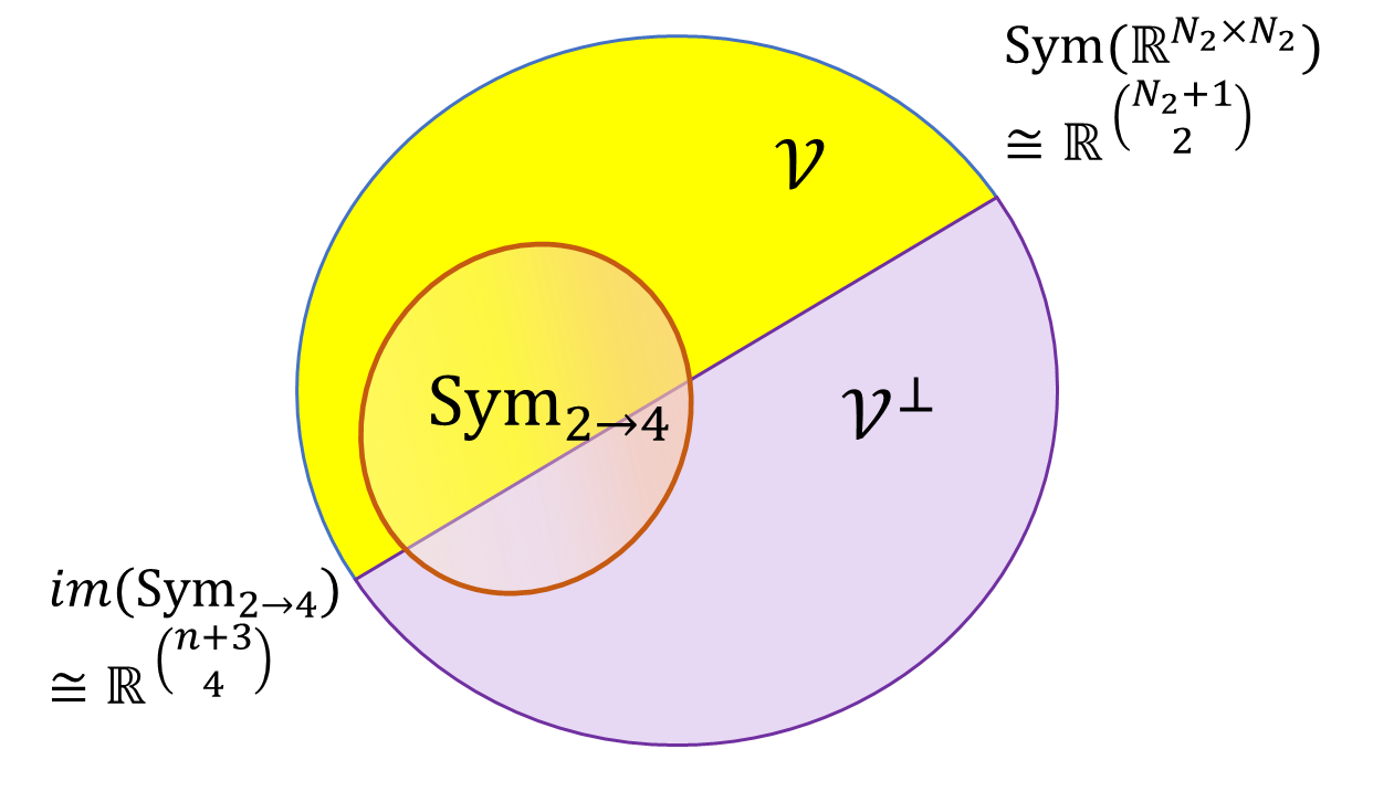
Figure 5: In this illustration, $N_{2}=\binom{n+1}{2}$ is the dimension of the space of homogeneous quadratic polynomials. The picture shows the space corresponding to the symmetric lift $(\mathbb{R}^{N_{2}})^{\circledast 2}\cong\mathsf{Sym}(\mathbb{R}^{N_{2}\times N_{2}})$ being expressed as $\mathcal{V}\oplus\mathcal{V}^{\perp}$, where $\mathcal{V}=(\mathcal{A}\circledast\mathcal{A})\oplus(\mathcal{A}\circledast\mathcal{A}^{\perp})$ as defined in (37). $\mathsf{Sym}_{2\to 4}$ denotes the orthogonal projector onto the space of fully symmetric tensors in $(\mathbb{R}^{n})^{\otimes 4}$. Lemma 8.4 shows that $\ker(\mathsf{Sym}_{2\to 4})\cap\mathcal{V}=\{0\}$ w.h.p. Note that $\mathsf{Sym}_{2\to 4}$ may not be a projection matrix when restricted to $\mathcal{V}$.

Lemma 8.4 ($\mathsf{Sym}_{2\to 4}$ does not annihilate any vector in $\mathcal{V}$ for smoothed instances).

Consider the following matrix $M\in\mathbb{R}^{\binom{n+3}{4}\times(mN_{2}-\binom{m}{2})}$ formed by columns

$$\text{columns}(M)= \left\{\mathsf{Sym}_{2\to 4}(A_{i}\otimes A_{j}+A_{j}\otimes A_{i}):1\leq i\leq j\leq m\right\}$$ (38)

$$\bigcup\left\{\mathsf{Sym}_{2\to 4}(A_{i}\otimes F_{j}+F_{j}\otimes A_{i}):1\leq i\leq m,m+1\leq j\leq N_{2}\right\}.$$

There exists a constant $c>0$, such that when $m<cN_{2}$, with probability at least $1-\exp(-\Omega(n))$, we have that $M$ has full column rank in a robust sense i.e.,

$$\sigma_{\min}(M)\geq\frac{\rho^{2}}{n^{O(1)}}.$$ (39)

Note that $\binom{m+1}{2}+m(N_{2}-m)=mN_{2}-\binom{m}{2}$ is the number of columns of the above matrix. . The above lemma shows that while $\mathsf{Sym}_{2\to 4}$ is an orthogonal projection matrix of rank $\binom{n+3}{4}$ acting on a space of dimension $\binom{N_{2}+1}{2}$ (which is larger by a constant factor $\approx 3$), it does not annihilate any vector in the vector space $\mathcal{V}$. In other words we show that $\ker(\mathsf{Sym}_{2\to 4})\cap\mathcal{V}=\{0\}$. See Figure 5 for an illustration. Moreover this is true in a robust sense. We now show why the above lemma suffices for the Proposition 8.3.

Proof of Proposition 8.3 from Lemma 8.4.

We know that $\sigma_{m}(A)\geq\rho/n^{O(1)}$ with probability $1-\exp(-\Omega(N_{2}))$, since $m<cN_{2}$. We condition on this event for the rest of the argument. The proof just follows from identifying the null space and a dimension counting argument. From the properties of $\mathsf{Sym}_{2\to 4}$ stated earlier, for any $v_{1},v_{2}\in\mathbb{R}^{N_{2}}\cong(\mathbb{R}^{n})^{\circledast 2}\cong\mathbb{R}^{N_{2}}$ we have

$$\mathsf{Sym}_{4}(v_{1}\otimes v_{2})=\mathsf{Sym}_{2\to 4}\Big{(}\frac{(v_{1}\otimes v_{2}+v_{2}\otimes v_{1})}{2}\Big{)}=\mathsf{Sym}_{2\to 4}(v_{1}\otimes v_{2}).$$

Hence, we can restrict to the subspace $\mathbb{R}^{N_{2}}\circledast\mathbb{R}^{N_{2}}$ as considered in Figure 5. Now we observe that

$$\forall w\in(\mathcal{A}^{\perp})\circledast(\mathcal{A}^{\perp}),v\in\mathcal{A}\circledast\mathbb{R}^{N_{2}}, ~{}\text{ we have }\langle w,v\rangle=0,~{}\text{i.e.,}$$ (40)

$$\forall j_{1},j_{2}\in\{m+1,\dots,N_{2}\},\forall i\in[m],v\in\mathbb{R}^{N_{2}}, ~{}\langle(F_{j_{1}}\otimes F_{j_{2}}+F_{j_{2}}\otimes F_{j_{1}}),(A_{i}\otimes v+v\otimes A_{i})\rangle=0.$$

The subspace $\mathcal{V}^{\perp}=\mathcal{A}^{\perp}\circledast\mathcal{A}^{\perp}$ has dimension $\binom{N_{2}-m+1}{2}$. The space orthogonal to this is exactly $\mathcal{V}$ and has dimension

$$\dim(\mathcal{V})=\binom{N_{2}+1}{2}-\binom{N_{2}-m+1}{2}=\frac{N_{2}(N_{2}+1)}{2}-\frac{(N_{2}-m)(N_{2}-m+1)}{2}=mN_{2}-\binom{m}{2}.$$

Moreover, each of the $mN_{2}-\binom{m}{2}$ columns of the matrix $M$ from (38) belong to the column space of the matrix $\mathrm{Sym}_{4}~{}\left(I_{N_{2}\times N_{2}}\otimes A\right)$ of Proposition 8.3. Hence Lemma 8.4 implies Proposition 8.3. ∎

Proof of Lemma 8.4 using random restrictions and contraction.

We now proceed to the proof of Lemma 8.4. We use the ideas we have developed in the previous sections to tackle the random matrix in Lemma 8.4. As in Section 5, we will view $\mathsf{Sym}_{2\to 4}$ as a tensor $W_{2\to 4}\in\mathbb{R}^{\binom{n+3}{4}\times N_{2}\times N_{2}}$; this tensor has rank $\binom{n+3}{4}$ when viewed as a flattened $\mathbb{R}^{\binom{n+3}{4}\times N_{2}^{2}}$ matrix. The random matrix in Lemma 8.4 is very similar to the random matrices analyzed in Section 5 through random contractions. However in this case, we are doing lopsided “random contractions” corresponding to $A^{\circledast 2}+A\otimes F$ where $A\in\mathbb{R}^{N_{2}\times m},F\in\mathbb{R}^{N_{2}\times(N-m)}$, and we want the entire set of $m\times N_{2}$ array of vectors in $R=\binom{n+3}{4}$ dimensions to be linearly independent in a robust sense. While there is a clear contraction along one mode ($N_{2}$ to $m\ll N_{2}$), there is no effective reduction in the dimension along the other mode (it remains $N_{2}$ since the concatenated matrix $[A,F]$ still has $N_{2}$ columns).

To tackle this, we will use a stronger property of the tensor $W_{2\to 4}$ (the tensor corresponding to the operator $\mathsf{Sym}_{2\to 4}$) that ensures that we can keep all of the dimensions corresponding to one of the modes. Consider the slices $W_{1},\dots,W_{N_{2}}\in\mathbb{R}^{R\times N_{2}}$ (it does not matter which of the last two modes we consider since it is symmetric), and let $\Pi_{-i}^{\perp}$ denote the projector perpendicular to the span of $\cup_{i^{\prime}\in[N_{2}]\setminus\{i\}}\mathrm{cols}(W_{i^{\prime}})$. We would like to argue that for all $i\in[N_{2}]$, $\Pi^{\perp}_{-i}W_{i}$ has a large rank of $\Omega(N_{2})$ in a robust sense i.e., $\forall i\in[N_{2}],~{}\sigma_{\Omega(N_{2})}(\Pi_{-i}^{\perp}W_{i})$ is inverse polynomial with high probability. However, this is unfortunately too good to be true.

The key idea here is to use the random restriction idea from Section 5.2. Set $\delta\coloneqq 1/16$. We define a random set $T\subseteq[N_{2}]$ such that each $i\in[N_{2}]$ belongs to $T$ independently with probability $\delta$ each. For each $i\in[N_{2}]$, let $W_{i,T}\in\mathbb{R}^{R\times T}$ denote the restriction of $W_{i}$ to the columns given by $T$. Similarly, let $\Pi_{-i,T}^{\perp}$ denote the (orthogonal) projection matrix that is perpendicular to the span of $\cup_{i^{\prime}\in[N_{2}]\setminus\{i\}}\mathrm{cols}(W_{i^{\prime},T})$. We show the following claim.

Claim 8.5.

(Large relative rank when random restricted to $T\subseteq[N_{2}]$) In the above notation, there is a constant $c\geq 1/64$ such that with probability $1-\exp(-\Omega(N_{2}))$ over the random choice of $T\subseteq[N_{2}]$

$$\forall i\in[N_{2}],~{}\sigma_{cN_{2}}(\Pi_{-i,T}^{\perp}W_{i,T})\geq 1,$$ (41)

where $\Pi_{-i,T}$ is the projector onto the span of the union of the columns of $W_{i^{\prime},T}$ for all $i^{\prime}\neq i$. In particular, there exists a $T\subseteq[N_{2}]$ such that (41) holds (deterministically).

Proof.

Set $\delta\coloneqq 1/16$. In this proof, we will have unordered $4$-tuples represented by multiset of the form $\{i_{1},i_{2},i_{3},i_{4}\}$ where $i_{1},\dots,i_{4}\in[n]$; similarly we will use multisets of the form $\{i_{1},i_{2}\}$ for unordered pairs. For example $\{1,3,3,5\}$ is the same as $\{3,5,1,3\}$. We will use the multiset $\{i_{1},i_{2},i_{3},i_{4}\}$ given by the canonical ordering $1\leq i_{1}\leq i_{2}\leq i_{3}\leq i_{4}\leq n$ to uniquely represent the unordered $4$-tuple. Note that some indices may be repeated.

Consider any $i=\{i_{1},i_{2}\}\in[N_{2}]$ where $1\leq i_{1}\leq i_{2}\leq n$. We will now argue about $\Pi_{-i,T}W_{i}$ Consider a fixed $j=\{j_{1},j_{2}\}\in T$ with $j_{1}\leq j_{2}$. Now the vector corresponding to $W(:,\{i_{1},i_{2}\},\{j_{1},j_{2}\})$ has exactly one entry that is $1$ corresponding to the index given by the unordered tuple $\{i_{1},i_{2},j_{1},j_{2}\}$, and $0$ otherwise. In other words, if $e_{i}$ refers to the $i$th standard basis vector (in appropriate dimensions), then $\mathsf{Sym}_{2\to 4}(e_{\{i_{1},i_{2}\}},e_{\{j_{1},j_{2}\}})=e_{\{i_{1},i_{2},j_{1},j_{2}\}}$. But there are at most $\binom{4}{2}-1$ other pairs $i^{\prime}\in[N_{2}],j^{\prime}\in[N_{2}]$ whose vectors $W(:,i^{\prime},j^{\prime})\in\mathbb{R}^{\binom{n+3}{4}}$ have a non-zero entry corresponding at the $\{i_{1},i_{2},j_{1},j_{2}\}$th index. Each of these other $\binom{4}{2}-1$ choices for $i^{\prime}=\{i^{\prime}_{1},i^{\prime}_{2}\}$ has its corresponding $j^{\prime}=\{j^{\prime}_{1},j^{\prime}_{2}\}$ present in $T$ with probability at most $\delta$ (note that $j^{\prime}\neq j$ since $i^{\prime}\neq i$, and hence conditioning on $j\in T$ does not affect whether $j^{\prime}\in T$). Hence, by a union bound, we have

$$\operatorname*{\mathbb{P}}\Big{[}(\Pi_{-i,T}^{\perp}W_{i})e_{\{i_{1},i_{2},j_{1},j_{2}\}}=e_{\{i_{1},i_{2},j_{1},j_{2}\}}\Big{]}\geq 1-\Big{(}\binom{4}{2}-1\Big{)}\delta\geq 1-5\delta.$$

Moreover the above event is independent for each $j=\{j_{1},j_{2}\}\in[N_{2}]$. The expected number of indices $j=\{j_{1},j_{2}\}$ which belong to $T$ and the above event holds is

$$\operatorname*{\mathbb{E}}\Big{[}\Big{|}\big{\{}\{j_{1},j_{2}\}\in[N_{2}]:\{j_{1},j_{2}\}\in T\text{ and }(\Pi_{-i,T}^{\perp}W_{i,T})e_{\{i_{1},i_{2},j_{1},j_{2}\}}=e_{\{i_{1},i_{2},j_{1},j_{2}\}}\big{\}}\Big{|}\Big{]}\geq\delta(1-5\delta)|N_{2}|\geq\delta/2|N_{2}|.$$

These unordered pairs $\{j_{1},j_{2}\}$ that satisfy $(\Pi_{-i,T}^{\perp}W_{i,T})e_{\{i_{1},i_{2},j_{1},j_{2}\}}=e_{\{i_{1},i_{2},j_{1},j_{2}\}}$ define an entire subspace of vectors $v$ such that $\lVert\Pi_{-i,T}^{\perp}W_{i,T}v\rVert\geq\lVert v\rVert$. Hence by the variational characterization of singular values and standard large deviation bounds we have that

$$\operatorname*{\mathbb{P}}\Big{[}\sigma_{\delta N_{2}/4}(\Pi_{-i,T}^{\perp}W_{i,T})\geq 1\Big{]}\geq 1-\exp(-\Omega(N_{2})).$$

By a union bound over $i\in[N_{2}]$, we get the statement of our claim.

∎

We now use Claim 8.5 along with contraction along the smoothed direction $A$ to get our final lemma. Recall $R=\binom{n+3}{4}$. Let $\Phi\in\mathbb{R}^{R\times N_{2}^{2}}$ denotes the natural matrix representation of $\mathsf{Sym}_{2\to 4}$ acting on $\mathbb{R}^{N_{2}^{2}}$ obtained by flattening $\mathsf{Sym}_{2\to 4}$ appropriately. Define the matrix $M\in\mathbb{R}^{R\times(\binom{m+1}{2}+m(N_{2}-m))}$ to be the block matrix

$$M=\Big{[}\Phi(A\circledast A)~{},~{}\Phi(A\otimes F)\Big{]}=\Phi\Big{[}A\circledast A~{},~{}A\otimes F\Big{]},$$

where $F\in\mathbb{R}^{N_{2}\times(N_{2}-m)}$ matrix with columns $F_{m+1},\dots,F_{N_{2}}$. To analyze the least singular value of $M$, we first need to apply the decoupling technique in used Lemma 5.9.

Let $A=B+Z_{1}+Z_{2}$ where $Z_{1},Z_{2}\in\mathbb{R}^{N_{2}\times m}$ are random Gaussian matrixes with independent entries $N(0,\rho_{1}^{2})$ and $N(0,\rho_{2}^{2})$ respectively with $\rho_{1}^{2}+\rho_{2}^{2}=\rho^{2}$. Then by the arguments in Lemma 5.9, it suffices to consider the matrix $M^{\prime}\in\mathbb{R}^{R\times mN_{2}}$ given below and prove an inverse polynomial lower bound on its least singular value. That is, we need to show that with probability at least $1-\exp(-\Omega(n))$

$$\sigma_{mN_{2}}\big{(}M^{\prime}\big{)}\geq\frac{\Omega(\rho)}{n^{O(1)}},\text{ where }M^{\prime}\coloneqq\Phi\Big{[}(B+Z_{1})\otimes(B+Z_{1}+2Z_{2})~{},~{}(B+Z_{1}+Z_{2})\otimes F\Big{]}.$$ (42)

The above bound (42) will follow from the following two simpler claims.

Claim 8.6.

In the above notation, the matrix $Q=[B+Z_{1}+2Z_{2}~{},~{}F]$ is full rank in a robust sense i.e., with probability $1-\exp(-\Omega(N_{2}))$

$$\sigma_{N_{2}}(Q)\geq\frac{c\rho}{n^{O(1)}},$$

for some absolute constant $c>0$.

Note that the matrix $[B+Z_{1}+Z_{2}~{},~{}F]=[A~{},~{}F]$ has inverse polynomial least singular value by design, since $F$ was chosen to complete the basis and $\sigma_{m}(A)$ is lower bounded w.h.p. We just need to show that adding the random matrix $[Z_{2}~{},~{}0]$ does not affect its least singular value. This is shown by rewriting the random matrices and a standard net argument in Appendix B. The second claim shows that after applying a random modal contraction with the random matrix $U=[B+Z_{1}~{},~{}Z_{2}]\in\mathbb{R}^{N_{2}\times(2m)}$, the matrix is well-conditioned.

Claim 8.7.

Let $U=[B+Z_{1}~{},~{}Z_{2}]$. Suppose the matrix $W\in\mathbb{R}^{R\times(2m\cdot N_{2})}$ is obtained by random modal contraction applied to $\mathsf{Sym}_{2\to 4}$ (along the second mode). Formally, suppose $\Phi_{1},\Phi_{2},\dots,\Phi_{N_{2}}\in\mathbb{R}^{R\times N_{2}}$ represent the matrix slices of $\Phi$, and suppose $\forall i\in[N_{2}]~{}W_{i}=\Phi_{i}U$ where random matrix $U=[B+Z_{1}~{},~{}Z_{2}]\in\mathbb{R}^{N_{2}\times(2m)}$. Then the matrix $W=[W_{1}~{}|~{}W_{2}~{}|~{}\dots~{}|~{}W_{N_{2}}]$ satisfies with probability at least $1-\exp(-\Omega(N_{2}))$ that $\sigma_{(2mN_{2})}\big{(}W\big{)}\geq c^{\prime}\rho/n^{c}$ for absolute constants $c,c^{\prime}>0$

The above Claim 8.7 follows directly by applying Lemma 5.5 along with Claim 8.5. We defer the proof to Appendix B.

With Claims 8.6 and 8.7 in hand we can now establish (42) complete the proof of Lemma 8.4. Consider the matrix $\widehat{M}\in\mathbb{R}^{R\times(2mN_{2})}$ given by

$$\widehat{M} =\Phi\Big{(}\big{[}B+Z_{1}~{},~{}Z_{2}\big{]}\otimes\big{[}(B+Z_{1}+2Z_{2})~{},~{}F\big{]}\Big{)},$$ (43)

$$=\Phi\Big{(}U\otimes Q\Big{)},$$

$$\text{ where }U =[B+Z_{1}~{},~{}Z_{2}]\in\mathbb{R}^{N_{2}\times(2m)},\text{ and }Q=[B+Z_{1}+2Z_{2}~{},~{}F]\in\mathbb{R}^{N_{2}\times N_{2}},$$

as defined in the earlier claims. Note that $M^{\prime}\in\mathbb{R}^{R\times mN_{2}}$ is a submatrix of $\widehat{M}\in\mathbb{R}^{R\times(2mN_{2})}$. Hence a least singular value bound on $\widehat{M}$ (note we show it has full column rank) implies the same least singular value bound for $M^{\prime}$. Suppose $W\in\mathbb{R}^{R\times(2mN_{2})}$ is the matrix defined in Claim 8.7 and $W^{(1)},\dots,W^{(2m)}\in\mathbb{R}^{R\times N_{2}}$ are corresponding blocks of $W$ that correspond to the matrix slices taken along the second mode of the tensor corresponding to $W$. Then up to rearranging columns

$$\widehat{M}\cong\Big{(}W^{(1)}Q~{},~{}W^{(2)}Q~{},~{}\dots~{},W^{(2m)}Q\Big{)}=\Big{(}W^{(1)}~{},~{}W^{(2)}~{},~{}\dots~{},W^{(2m)}\Big{)}\Big{(}I_{2m\times 2m}\otimes Q\Big{)}.$$ (44)

We condition on the success events in both Claim 8.6 and Claim 8.7; by a union bound, they both hold with probability at least $1-2\exp(-\Omega(n))$. From Claim 8.7, the matrix $W$ defined in Claim 8.7 has

$$\sigma_{2mN_{2}}\Big{(}W^{(1)}~{},~{}W^{(2)}~{},~{}\dots~{},W^{(2m)}\Big{)}=\sigma_{2mN_{2}}\big{(}W\big{)}\geq\frac{c^{\prime}\rho}{n^{O(1)}}.$$ (45)

From Claim 8.6,

$$\sigma_{2mN_{2}}\Big{(}I_{2m\times 2m}\otimes Q\Big{)}=\sigma_{N_{2}}(Q)\geq\frac{c^{\prime\prime}\rho}{n^{O(1)}}.$$ (46)

Combining (44), (45) and (46), we finish the proof of the lemma. ∎

9 Application: Subspace Clustering

Very recently, Chandra, Garg, Kayal, Mittal, and Sinha [CGK⁺24] extended the framework of [GKS20] and obtained robust analogs of the corresponding learning algorithms. One of the applications they consider is subspace clustering, in which there are $s$ underlying hidden $t$-dimensional subspaces $W_{1},\dots,W_{s}$. We see a set of points $A$ such that $A=A_{1}\cup\dots\cup A_{s}$, where each $A_{i}\subseteq W_{i}$. Our goal is to recover the $W_{i}$ from $A$.

[CGK⁺24] give an algorithm for this problem by reducing to robust vector space decomposition. For a specific block $i$, let $V_{i}=\left[\mathbf{v}_{i1},\dots,\mathbf{v}_{it}\right]$ be a basis for $W_{i}$. Treating each $a^{\circledast d}$ as a homogeneous degree-$d$ polynomial, they take all first-order partial derivatives of all of the $a^{\circledast d}$. Note that if $a\in A_{i}$, then $a^{\circledast d}\in\mathrm{colspan}(V_{i}^{\circledast d})$, and the first order partial derivatives of $a^{\circledast d}$ are in $\mathrm{colspan}(V_{i}^{\circledast(d-1)})$.

This sets up the problem in the framework of vector space decomposition. In vector space decomposition, we are given two vector spaces $U$ and $V$, where there are hidden decompositions $U=U_{1}\oplus\dots\oplus U_{s}$ and $V=V_{1}\oplus\dots\oplus V_{s}$, where $\oplus$ denotes a direct sum. We are also have a set of linear maps $\mathfrak{B}=(B_{1},\dots,B_{\ell})$, where each $B_{j}:U\rightarrow V$, while respecting that $B_{j}U_{i}\subseteq V_{i}$ for all $i$. The goal of vector space decomposition is to recover the $U_{i}$ (and therefore the $V_{i}$) given $U,V,$ and $\mathfrak{B}$.

In the case of subspace clustering, we can take $U$ to be the span of $\{a^{\circledast d}:a\in A\}$, $\mathfrak{B}$ to be the set maps corresponding to first-order partial derivatives, and $V$ to be the image space of $\mathfrak{B}$ applied to $U$. Then, as long as subspaces $\mathrm{colspan}\left(V_{i}^{\circledast(d-1)}\right)$ are linearly independent, and some non-degeneracy conditions on the set of points $A$ are met, this set of linear maps allows us to recover the subspaces $V_{i}$ via robust vector space decomposition.

[CGK⁺24] assume two conjectures to prove that this algorithm succeeds in the smoothed framework. The first is a smoothed version of the statement that the subspaces $\mathrm{colspan}(V_{i}^{\circledast(d-1)})$ are linearly independent. We address this first conjecture in Section 9.1. The second conjecture is that for sufficiently many perturbed points $A_{i}$ from subspace $W_{i}$, the set $\{a^{\circledast d}:a\in A_{i}\}$ spans $W_{i}^{\circledast d}$ robustly. We address this second conjecture in Section 9.2.

9.1 Proof of Conjecture on Robust Linear Independence of Subspace Lifts

Conjecture 9.1 (Conjecture 1.1 in [CGK⁺24]).

Given $\delta>0$ and $d\in\mathbb{N}$, fix $m<n$ ($m$ is the dimension of the subspaces), $s$ such that $s\binom{m+d-1}{d}\leq\delta\binom{n+d-1}{d}$. Additionally assume that $m\leq(1-\delta)c_{d}n$, where $c_{d}$ is as in Corollary 5.3.

For each $i\in[s]$, let $V_{i}$ be an orthonormal basis for the subspace $\widehat{W}_{i}$. Each $\widehat{W}_{i}$ is the subspace spanned by $P_{i}+G_{i}\in\mathbb{R}^{n\times m}$, where $P_{i}\in\mathbb{R}^{n\times m}$ is an arbitrary matrix with orthonormal columns, and $G_{i}\sim\mathcal{N}(0,\rho^{2}/n)^{n\times t}$ is drawn independently for each $i\in[s]$.

Let $M=\left[M_{1}\ M_{2}\ \dots\ M_{s}\right]$ be a matrix formed of $s$ blocks, where

$$M_{i}=V_{i}^{\circledast d}.$$

Then with probability at least $1-\exp(-\Omega_{d,\delta}(n))$, the least singular value of $M$ is bounded as

$$\sigma_{\mathrm{min}}(M)=\sigma_{s\binom{m+d-1}{d}}(M)\geq\mathrm{poly}(\rho,1/n).$$

To prove this conjecture we start with a lemma that lets us to reduce to the setting of Corollary 5.3.

Lemma 9.2.

Fix $\ell,k,s\in\mathbb{N}$ and $\varepsilon,\eta,L\geq 0$. Let $A_{1},\dots,A_{s},U_{1},\dots,U_{s}\in\mathbb{R}^{\ell\times k}$ be matrices that for all $i=1,\dots,s$ we have

$$\mathrm{colspan}(A_{i})=\mathrm{colspan}(U_{i})\qquad\mathrm{and}\qquad\|A_{i}\|_{2}\leq L\qquad\mathrm{and}\qquad\sigma_{\min}(U_{i})\geq\eta.$$

Additionally assume that $\sigma_{\min}([A_{1}\ \dots\ A_{s}])\geq\varepsilon$. Then we have

$$\sigma_{\min}([U_{1}\ \dots\ U_{s}])\geq\frac{\eta\varepsilon}{L}.$$

Proof.

Suppose towards a contradiction that there is a unit vector $v=v_{1}\oplus\dots\oplus v_{s}\in\mathbb{R}^{sk}$ such that

$$\|[U_{1}\ U_{2}\ \dots\ U_{s}]v\|=\left\|\sum_{i=1}^{s}U_{i}v_{i}\right\|<\frac{\eta\varepsilon}{L}.$$

Then, since $\mathrm{colspan}(A_{i})=\mathrm{colspan}(U_{i})$ for each $i$, it follows that for each $i=1,\dots,s$, there exists a vector $z_{i}\in\mathbb{R}^{k}$ such that $U_{i}v_{i}=A_{i}z_{i}$. Set $z=z_{1}\oplus\dots\oplus z_{s}$. Then we have

$$\|[A_{1}\ \dots\ A_{s}]z\|=\sqrt{\sum_{i=1}^{s}\|A_{i}z_{i}\|^{2}}=\sqrt{\sum_{i=1}^{s}\|U_{i}v_{i}\|^{2}}=\|[U_{1}\ \dots\ U_{s}]v\|<\frac{\eta\varepsilon}{L}.$$

Furthermore, for each $i$ we find that

$$\eta\|v_{i}\|\leq\|U_{i}v_{i}\|=\|A_{i}z_{i}\|\leq L\|z_{i}\|,$$

hence

$$\|z_{i}\|\geq\frac{\eta\|v_{i}\|}{L},\qquad\mathrm{which\ implies}\qquad\frac{1}{\|z\|}\leq\frac{L}{\eta}.$$

We then obtain that

$$\left\|[A_{1}\ \dots\ A_{s}]\frac{z}{\|z\|}\right\|=\frac{1}{\|z\|}\|[A_{1}\ \dots\ A_{s}]z\|<\frac{L}{\eta}\frac{\eta\varepsilon}{L},$$

which contradicts the assumption that $\sigma_{\min}([A_{1}\ \dots\ A_{s}])\geq\varepsilon$. ∎

We now prove Conjecture 9.1.

Proof.

For each $i=1,\dots,s$, set $\tilde{P}_{i}:=P_{i}+G_{i}$. From Corollary 5.3, we have that with probability at least $1-\exp(-\Omega_{d,\delta}(n))$ that

$$\sigma_{\min}([\tilde{P}_{1}^{\circledast d}\ \dots\ \tilde{P}_{s}^{\circledast d}])\geq\frac{\rho^{d}}{\sqrt{t}n^{O(d)}}.$$

Furthermore, for each $i$, we have with probability at least $1-\exp(-\Omega(n)),$ that

$$\|\tilde{P}_{i}\|\leq 1+\rho c_{1}\sqrt{n},$$

for some $c_{1}>0$. For the remainder of the proof, we condition on these events.

Now, since $\tilde{P}_{i}$ has the same range as $V_{i}$, we also have that $\tilde{P}_{i}^{\circledast d}$ has the same range as $V_{i}^{\circledast d}$ for each $i$. Furthermore, since each $V_{i}$ is an orthogonal matrix and since $V_{i}^{\circledast d}=V_{i}^{\otimes d}\mathrm{Perm}_{\text{avg}}$ and the matrix $\mathrm{Perm}_{\text{avg}}$ has singular values in $[1/\sqrt{d!},1]$, we obtain that $\sigma_{\min}(V_{i})\geq 1/\sqrt{d!}$ for each $i=1,\dots,s$. Therefore, we can apply Lemma 9.2 to conclude that

$$\sigma_{\min}([V_{1}^{\circledast d}\ \dots\ V_{s}^{\circledast d}])\geq\frac{\rho^{d}}{(1+\rho c_{1}\sqrt{n})\sqrt{t(d!)}n^{O(d)}},$$

as claimed. ∎

9.2 Proof of the “Spanning” Conjecture of Subspace Lifts

[CGK⁺24] also conjecture that if we have smoothed vectors $\{\tilde{u}_{i}\}_{i=1}^{N}$ in $\mathbb{R}^{d}$, and if $N$ is large enough, then the polynomials $\langle\tilde{u}_{i},x\rangle^{r}$ are all “robustly” linearly independent. Formally, they conjecture the following:

Conjecture 9.3 (Conjecture 1.2 in [CGK⁺24]).

Suppose $\sigma,\delta>0$ are constants, and let $r\geq 1$ be an integer. Let $\{\tilde{u}_{i}\}_{i=1}^{N}$ be independent $\sigma$-perturbations of some (arbitrary) vectors $\{u_{i}\}_{i=1}^{N}$ of norm $\leq\Delta$. Suppose also that $N>(1+\delta)\binom{d+r-1}{r}$, and let $M$ be the $N\times\binom{d+r-1}{r}$ matrix whose $i$th row contains the vector of coefficients for the polynomial $\langle\tilde{u}_{i},x\rangle^{r}$. Then with high probability,

$$\sigma_{\binom{d+r-1}{r}}(M)\geq\mathrm{poly}_{r}\left(\frac{\sigma\delta}{n\Delta}\right).$$

We give a short and self-contained proof of this conjecture, but with a weaker guarantee on $N$. Specifically, we show that the conclusion holds as long as

$$N\geq 2r\binom{d+r-1}{r}.$$ (47)

The main ingredient is the observation that for any unit vector $a\in\mathbb{R}^{\binom{d+r-1}{r}}$, $\langle M^{(i)},a\rangle$ is large enough with high probability, where $M^{(i)}$ is the $i$th row of $M$, and the probability is over the choice of the randomness in $\tilde{u}_{i}$. I.e.,

Lemma 9.4.

Suppose $a\in\mathbb{R}^{\binom{d+r-1}{r}}$ is a unit vector that we index using $r$-sized multisets $I$ of $[d]$. Let $x\in\mathbb{R}^{n}$ be an arbitrary vector, and let $\tilde{x}$ be an entrywise $\sigma$ perturbation, for some $\sigma>0$. In other words, $\tilde{x}_{i}:=x_{i}+g_{i}$, where $g_{i}\sim\mathcal{N}(0,\sigma^{2})$. Finally, denote $f(\tilde{x})=\sum_{I}a_{I}\prod_{i\in I}\tilde{x}_{i}$. Then for any $y$ and any $\varepsilon>0$, we have

$$\operatorname*{\mathbb{P}}[|f(\tilde{x})-y|<\varepsilon]<\frac{c^{\prime}r}{\sigma}\varepsilon^{1/r},$$

for some absolute constant $c^{\prime}$.

The Lemma is very similar to the classic Carbery-Wright inequality, but unfortunately it is not a direct consequence, because the Carbery-Wright inequality requires a bound on the variance of $f$. Fortunately, it turns out that one can always obtain a lower bound on the variance in terms of the $\ell_{2}$ norm of the coefficient vector.

Proof.

As noted above, we first apply the main result from the recent work of [GM22] to lower bound the variance of $f$. To this end, note that $f(\tilde{x})$ is a homogeneous polynomial in the variables $\tilde{x}_{i}$, whose distributions are independent, according to appropriately shifted Gaussians. For this setting, [GM22] prove that

$$\text{Var}(f(\tilde{x}))\geq\frac{\sigma^{2r}}{B^{r}}\cdot\sum_{I}a_{I}^{2},$$

where $B$ is a universal constant (which they upper bound by $2^{15}$, but is likely much smaller for Gaussians). Next, we apply Carbery-Wright inequality [CW01], which states that for any $y\in\mathbb{R}$ and $\varepsilon>0$,

$$\operatorname*{\mathbb{P}}[|f(\tilde{x})-y|<\varepsilon]\leq cr\frac{\varepsilon^{1/r}}{\text{Var}(f)^{1/2r}},$$

for some absolute constant $c$. Combining this with the lower bound on the variance and noting that $\lVert a\rVert=1$, we obtain:

$$\operatorname*{\mathbb{P}}[|f(\tilde{x})-y|<\varepsilon]\leq\frac{c^{\prime}r}{\sigma}\varepsilon^{1/r}$$

for some absolute constant $c^{\prime}$. This completes the proof of the lemma. ∎

We can now prove the conjecture via a standard $\varepsilon$-net argument. We also condition on the event that $\lVert M\rVert$ is upper bounded by $\text{poly}_{r}(n\Delta)$. This can easily be checked to hold with extremely high probability.

Proof of Conjecture 9.3 assuming (47).

For any unit vector $a\in\mathbb{R}^{\binom{d+r-1}{r}}$, Lemma 9.4 bounds the probability of one of the entries of $Ma$ being of small norm. Since the rows of $M$ all have independent randomness, we have, for any $\varepsilon>0$,

$$\operatorname*{\mathbb{P}}[\lVert Ma\rVert<\varepsilon]<\left(\frac{c^{\prime}r}{\sigma}\varepsilon^{1/r}\right)^{N}.$$

Let us write $C=\frac{c^{\prime}r}{\sigma}$, for convenience, so the RHS above becomes $(C\varepsilon^{1/r})^{N}$; also, write $D=\binom{d+r-1}{r}$.

Let $\delta>0$ be a parameter we will choose later, and let $\mathcal{N}_{\delta}$ be a $\delta$ net for unit vectors in $\mathbb{R}^{D}$. As is well known, we may assume that $|\mathcal{N}_{\delta}|\leq\left(\frac{4}{\delta}\right)^{D}$. By a union bound, we have that

$$\operatorname*{\mathbb{P}}[\lVert Ma\rVert\geq\varepsilon~{}\forall a\in\mathcal{N}_{\delta}]\geq 1-|\mathcal{N}_{\delta}|(C\varepsilon^{1/r})^{N}.$$

If we can ensure that this event occurs, we also have that for all unit vectors $a$, $\lVert Ma\rVert\geq\varepsilon-\delta\lVert M\rVert$, where $\lVert M\rVert$ is the spectral norm of $M$. First, we set $\delta=\frac{\varepsilon}{2\lVert M\rVert}$, which ensures a lower bound of $\varepsilon/2$ on the least singular value. Now for the high probability bound to hold, we require

$$\left(C\varepsilon^{1/r}\right)^{N}\left(\frac{4}{\delta}\right)^{D}\ll 1\iff\left(C\varepsilon^{1/r}\right)^{N}\left(\frac{8\lVert M\rVert}{\varepsilon}\right)^{D}\ll 1.$$

Now, by assumption (47), we have $N\geq 2rD$. Since adding more rows to $M$ only improves the least singular value, let us assume that $N=2rD$. The equation above simplifies to $C^{2r}\varepsilon\cdot 8\lVert M\rVert\ll 1$, which holds if we set $\varepsilon=\frac{1}{16C^{2r}\lVert M\rVert}$.

This completes the proof of the conjecture. Indeed, we see that the failure probability in this case is exponentially small in $D$. ∎

Appendix A Auxiliary Lemmas

Lemma A.1.

Let $\tilde{u}\in\mathbb{R}^{n}$ be a $\rho$-smoothed vector and fix $\delta>0$. There exists a universal constant $c>0$ such that

$$Pr[\|\tilde{u}\|<\delta]\leq\Big{(}\frac{c\delta}{\rho}\Big{)}^{n}$$

Proof.

The PDF of $\tilde{u}$ is bounded above by $\left(\rho\sqrt{2\pi})^{-n}\right)$ from which we obtain that

$$Pr[\|\tilde{u}\|<\delta] \leq\int_{B(0,\delta)}\left(\rho\sqrt{2\pi}\right)^{-n}dx=\left(\rho\sqrt{2\pi}\right)^{-n}\mathrm{vol}\big{(}B(0,\delta)\big{)}$$

$$=\left(\rho\sqrt{2\pi}\right)^{-n}\frac{\left(\delta\sqrt{\pi}\right)^{n}}{\Gamma\left(\frac{n}{2}+1\right)}=\left(\frac{\delta}{\rho\sqrt{2}}\right)^{n}\frac{1}{\Gamma(\frac{n}{2}+1)}.$$

Now, using Stirling’s approximation we have

$$\Gamma\left(\frac{n}{2}+1\right)\geq\sqrt{\pi n}\left(\sqrt{\frac{n}{2e}}\right)^{n}.$$

Substituting this probability in above gives the desired probability upper bound. ∎

Block leave-one-out bounds and least singular value of smoothed matrices

Lemma A.2.

Let $U_{1},\dots,U_{t}\in\mathbb{R}^{n\times m}$ and for each $j=1,\dots,t$ let $\Pi^{\perp}_{-j}$ be the projection on to the orthogonal complement of

$$\mathrm{Ran}\left(\begin{bmatrix}U_{1}&\dots&U_{j-1}&U_{j+1}&\dots U_{t}.\end{bmatrix}\right)$$

Define $\ell_{B}(\{U_{j}\})=\min_{j}\sigma_{\min}(\Pi^{\perp}_{-j}U_{j}).$ Then

$$\frac{\ell_{B}(\{U_{j}\})}{\sqrt{t}}\leq\sigma_{\min}\left(\begin{bmatrix}U_{1}&\dots&U_{t}\end{bmatrix}\right)\leq\ell_{B}(\{U_{j}\}).$$

Proof.

Let $\alpha\in\mathbb{R}^{tm}$ be a unit vector and write $\alpha=\alpha_{1}\oplus\dots\oplus\alpha_{t}$. Intuitively, $\alpha_{j}$ records the entries of alpha that are coefficients of the columns of $U_{j}$ in the product $\begin{bmatrix}U_{1}&\dots&U_{t}\end{bmatrix}\alpha.$ Since $\alpha$ is a unit vector, there must exist some index $j$ such that $\|\alpha_{j}\|\geq\frac{1}{\sqrt{t}}$. From this we obtain

$$\left\|\Pi^{\perp}_{-j}U_{j}\alpha_{j}\right\|=\left\|\Pi^{\perp}_{-j}\begin{bmatrix}U_{1}&\dots&U_{t}\end{bmatrix}\alpha\right\|\leq\left\|\begin{bmatrix}U_{1}&\dots&U_{t}\end{bmatrix}\alpha\right\|.$$

Using the fact our lower bound on the norm of $\alpha_{j}$ and the fact that $\ell_{B}(\{U_{j}\})$ lower bounds the least singular value of $\Pi^{\perp}_{-j}U_{j}$, we obtain

$$\frac{\ell_{B}(\{U_{j}\})}{\sqrt{t}}\leq\left\|\Pi^{\perp}_{-j}U_{j}\alpha_{j}\right\|$$

from which the desired lower bound follows. The proof of the upper bound is straightforward. ∎

Lemma A.3.

Let $V\in\mathbb{R}^{n\times k}$ be an arbitrary matrix with $k\leq n$, and let $\tilde{V}$ be a $\rho$ perturbation. Suppose $\alpha_{i}$ are some scalars such that $\alpha_{i}\geq\delta$ for all $i\leq k$. Then for any $h\in(0,1/2)$,

$$\operatorname*{\mathbb{P}}\left[\sigma_{k/2}\left(\tilde{V}\text{diag}(\alpha)\right)<h\sigma\delta\right]\leq\exp(-\frac{1}{8}kn\log(1/h)).$$

Proof.

Let us denote $W=\tilde{V}\text{diag}(\alpha)$, for convenience. Suppose that $\sigma_{k/2}(W)<h\sigma\delta$. This implies that there exists a set $J$ of $k/2$ columns of $W$ with the property that the rest of the columns together have a squared projection at most $k^{2}(h\sigma\delta)^{2}$ orthogonal to the span of the columns in $J$.

Now take any subset of columns $J$ with $|J|=k/2$; the probability that any column $i\not\in J$ has a projection of length $<h\delta\rho$ orthogonal to the span of $J$ is at most $h^{n-\frac{k}{2}}$. (This is because for each of the $n-\frac{k}{2}$ directions orthogonal to the span of $J$, we must have a component $<h\delta\rho$, and we can use the standard Gaussian anticoncentration for each direction.) Since there are $k/2$ columns $i\not\in J$, the probability that all of them satisfy the condition is $\leq h^{\frac{k}{2}(n-\frac{k}{2})}$.

The total number of choices for $J$ is clearly at most $2^{k}$, thus taking a union bound, we have that the probability is at most

$$2^{k}h^{\frac{k}{2}(n-\frac{k}{2})}\leq\exp(-\frac{1}{8}kn\log(1/h)).$$

∎

Proof of Lemma 6.6

Proof.

Let $U\in\mathbb{R}^{n\times k}$ be a matrix whose columns form an orthonormal basis for $S$. We can now apply Lemma 5.7 to $U^{T}$ to conclude that there exists a subset $J$ of the rows of $U$ such that $\sigma_{k}(U_{|J})\leq 1/\sqrt{nk}$. [Here, $U_{|J}$ refers to the matrix $U$ restricted to the rows $J$.]

Now this implies that every vector in the column span of $U_{|J}$ can be expressed as $U_{|J}\alpha$, where $\alpha\in\mathbb{R}^{k}$ and $\lVert\alpha\rVert\leq\sqrt{nk}$. In particular, we can conclude that the vector with $1/\sqrt{k}$ in all $k$ coordinates can be so expressed. By considering $\alpha^{\prime}=\frac{\alpha}{\lVert\alpha\rVert}$, we have that $U\alpha^{\prime}$ has entries $\geq\frac{1}{\sqrt{k}\lVert\alpha\rVert}\geq\frac{1}{k\sqrt{n}}$ in all the entries corresponding to $J$.

Noting that $|J|=k$ completes the proof. ∎

Appendix B Proofs of Claims in Section 8 for Power Sum Decompositions

Claim B.1.

[Same as Claim 8.7] Let $U=\big{(}B+Z_{1}~{},~{}Z_{2}\big{)}$. Suppose the matrix $W\in\mathbb{R}^{R\times(2m\cdot N_{2})}$ is obtained by random modal contraction applied to $\mathsf{Sym}_{2\to 4}$ (along the second mode). Formally, suppose $\Phi_{1},\Phi_{2},\dots,\Phi_{N_{2}}\in\mathbb{R}^{R\times N_{2}}$ represent the matrix slices of $\Phi$, and suppose $\forall i\in[N_{2}]~{}W_{i}=\Phi_{i}U$ where random matrix $U=[B+Z_{1}~{},~{}Z_{2}]\in\mathbb{R}^{N_{2}\times(2m)}$. Then the matrix $W=[W_{1}|W_{2}|\dots|W_{N_{2}}]$ satisfies with probability at least $1-\exp(-\Omega(N_{2}))$ that $\sigma_{2mN_{2}}(W)\geq c^{\prime}\rho/n^{c}$ for absolute constants $c,c^{\prime}>0$

Proof.

We will use Claim 8.5 with the matrix $\Phi$. Let $T\subseteq[N_{2}]$ be any subset that satisfies (41). Set $s=N_{2},\varepsilon=\delta/4,k=|T|$. We will set the matrix $A_{1}=\Phi_{1,T},\dots,A_{N_{2}}=\Phi_{N_{2},T}$. Let $\tilde{U}=U_{T}$ (rows restricted to $T$) and let $U^{\prime}=U_{[N_{2}]\setminus T}$; note that they are mutually independent. For each $i\in[N_{2}]$, $C_{i}=\Phi_{i,[N_{2}]\setminus T}U^{\prime}$. For each $i\in[N_{2}]$, $W_{i}=C_{i}+A_{i}\tilde{U}$. Hence applying Lemma 5.5 we get the claim. ∎

Claim B.2.

[Same as Claim 8.6] The matrix $Q=(B+Z_{1}+2Z_{2}~{},~{}F)$ is full rank in a robust sense i.e., with probability $1-\exp(-\Omega(N_{2}))$

$$\sigma_{N_{2}}(Q)\geq\frac{c\rho}{n^{O(1)}},$$

for some absolute constant $c>0$.

Proof.

Let $Q_{1}=\big{(}B+Z_{1}+Z_{2}~{},~{}F\big{)}\in\mathbb{R}^{N_{2}\times N_{2}}$ and $Q_{2}=(Z_{2}~{},~{}0)\in\mathbb{R}^{N_{2}\times N_{2}}$. First we note that with probability $1-\exp(-\Omega(N_{2}))$, there exists constants $c_{1},c_{2}>0$ such that

$$\sigma_{N_{2}}(Q_{1})=\sigma_{N_{2}}\big{(}B+Z_{1}+Z_{2}~{},~{}F\big{)}=\sigma_{N_{2}}(A,F)\geq\frac{c_{2}\rho}{n^{c_{1}}}\eqqcolon\tau\rho.$$

This is because $\sigma_{m}(A)\geq\frac{\rho}{n^{\Omega(1)}}$ with high probability by standard random matrix theory, and since $F$ was chosen to complete the basis. We just need to show that adding the random matrix $Q_{2}$ does not affect decrease its least singular value by a lot.

Recall $Z_{1}\sim N(0,\rho_{1}^{2})^{N_{2}\times m},Z_{2}\sim N(0,\rho_{2}^{2})^{N_{2}\times m}$. Next we rewrite the random matrices $Z_{1}+2Z_{2}$ and $Z_{2}$ as follows after Gram-Schmidt orthogonalization. Suppose $Y_{1},Y_{2}\in\mathbb{R}^{N_{2}\times m}$ are random matrices with independent entries given by

$$Y_{1}\sim_{iid} N(0,\lambda_{1}^{2})^{N_{2}\times m},~{}Y_{2}\sim_{iid}N(0,\lambda_{2}^{2})^{N_{2}\times m},\text{ where }\lambda_{1}^{2}=\rho_{1}^{2}+\rho_{2}^{2},\lambda_{2}^{2}=\frac{\rho_{1}^{2}\rho_{2}^{2}}{\rho_{1}^{2}+\rho_{2}^{2}},$$

$$Z_{1}+Z_{2}= Y_{1},\text{ and }Z_{2}=\tfrac{\rho_{2}^{2}}{\rho_{1}^{2}+\rho_{2}^{2}}Y_{1}+Y_{2},\text{ i.e., }Y_{2}=\tfrac{1}{\rho_{1}^{2}+\rho_{2}^{2}}(\rho_{2}^{2}Z_{1}-\rho_{1}^{2}Z_{2})$$ (48)

Note that $Y_{1}$ and $Y_{2}$ are mutually independent (these are Gaussian r.v.s, and one can verify entrywise that their correlation is $0$). Let $\gamma=\rho_{2}^{2}/(\rho_{1}^{2}+\rho_{2}^{2})$. Note that $\gamma\in[c_{5}N_{2}^{-c_{4}},c_{6}N_{2}^{c_{4}}]$ for some constants $c_{4},c_{5},c_{6}>0$. We know that $Q_{1}=(B+Y_{1}~{}|~{}F)$ and $Q_{2}=(\gamma Y_{1}+Y_{2}~{}|~{}0)$.

In the rest of this proof we condition on $\sigma_{N_{2}}(Q_{1})\geq$ Consider any test unit vector $\alpha\in\mathbb{R}^{N_{2}}$, and let $\alpha_{[m]}$ be the restriction to the first $m$ coordinates. We will now show that for any constant $C>0$, $\lVert Q\alpha\rVert\geq\Omega(\rho^{2}/n^{O(C)})$ with probability $1-\exp(-CN_{2}\log(N_{2}))$. We have

$$Q\alpha=Q_{1}\alpha+\gamma Y_{1}\alpha_{[m]}+Y_{2}\alpha_{[m]},\text{ where }\lVert Q_{1}\alpha\rVert_{2}\geq\tau\rho.$$

We know further that with high probability $\lVert Y_{1}\rVert,\lVert Y_{2}\rVert\leq c^{\prime}\rho\sqrt{N_{2}}$ for some constant $c^{\prime}>0$. We split into two cases depending on whether (a) $\lVert\alpha_{[m]}\rVert_{2}\leq\tau/(2c^{\prime}(1+\gamma)\sqrt{N_{2}})$, or (b) otherwise.

In case (a), we have

$$\lVert Q\alpha\rVert_{2}\geq\lVert Q_{1}\alpha\rVert_{2}-\lVert\gamma Y_{1}\alpha_{[m]}\rVert_{2}-\lVert Y_{2}\alpha_{[m]}\rVert_{2}\geq\tau\rho-c^{\prime}\sqrt{N_{2}}\rho(\gamma+1)\lVert\alpha_{[m]}\rVert_{2}\geq\frac{\tau}{2}.$$

In case (b) $\lVert\alpha_{[m]}\rVert_{2}\geq\tau/(2c^{\prime}(1+\gamma)\sqrt{N_{2}})$. We use the anticoncentration from the Gaussian r.v. $Y_{2}\alpha_{[m]}$. Let $\beta=Q_{1}\alpha+\gamma Y_{1}\alpha_{[m]}\in\mathbb{R}^{N_{2}}$. For matrices $Q,Y_{2}\in\mathbb{R}^{N_{2}\times m}$, let $Q(i),Y_{2}(i)\in\mathbb{R}^{m}$ represent the $i$th rows. We have for some absolute constant $c_{7}>0$

$$\operatorname*{\mathbb{P}}\Big{[}\lVert Q\alpha\rVert_{2}\leq\varepsilon\Big{]} \leq\operatorname*{\mathbb{P}}\Big{[}\forall i\in[N_{2}],|\langle Q(i),\alpha\rangle|\leq\varepsilon\Big{]}=\operatorname*{\mathbb{P}}\Big{[}\forall i\in[N_{2}],|\beta_{i}+\langle Y_{2}(i),\alpha_{[m]}\rangle|\leq\varepsilon\Big{]}$$

$$=\operatorname*{\mathbb{P}}_{\begin{subarray}{c}g_{1},\dots,g_{N_{2}}\sim_{iid}\\ N(0,\lambda_{2}\lVert\alpha_{[m]}\rVert)\end{subarray}}\Big{[}\forall i\in[N_{2}],~{}|\beta_{i}+g_{i}|\leq\varepsilon\Big{]}$$

$$\leq\Big{(}\frac{\varepsilon\cdot(1+\gamma)\sqrt{N_{2}}}{c_{7}\lambda_{2}\tau}\Big{)}^{N_{2}}\leq N_{2}^{-CN_{2}},$$

by setting $\varepsilon$ appropriately as $\varepsilon=c_{7}\tau\lambda_{2}/((1+\gamma)N_{2}^{C+1})$, which is still inverse polynomial in $N_{2}$. Now by doing a standard union bound argument over a net of $\alpha\in\mathbb{R}^{N_{2}}$, the claim follows. ∎

References

- [ADM+18] Nima Anari, Constantinos Daskalakis, Wolfgang Maass, Christos Papadimitriou, Amin Saberi, and Santosh Vempala. Smoothed analysis of discrete tensor decomposition and assemblies of neurons. In Advances in Neural Information Processing Systems, 2018.
- [AGH+15] Anima Anandkumar, Rong Ge, Daniel J. Hsu, Sham M. Kakade, and Matus Telgarsky. Tensor decompositions for learning latent variable models (A survey for ALT). In Kamalika Chaudhuri, Claudio Gentile, and Sandra Zilles, editors, Algorithmic Learning Theory - 26th International Conference, ALT 2015, Banff, AB, Canada, October 4-6, 2015, Proceedings, volume 9355 of Lecture Notes in Computer Science, pages 19–38. Springer, 2015.
- [AHK12] Animashree Anandkumar, Daniel J. Hsu, and Sham M. Kakade. A method of moments for mixture models and hidden markov models. In Shie Mannor, Nathan Srebro, and Robert C. Williamson, editors, COLT 2012 - The 25th Annual Conference on Learning Theory, June 25-27, 2012, Edinburgh, Scotland, volume 23 of JMLR Proceedings, pages 33.1–33.34. JMLR.org, 2012.
- [AK08] Baruch Awerbuch and Robert Kleinberg. Online linear optimization and adaptive routing. Journal of Computer and System Sciences, 74(1):97–114, 2008.
- [AMP16] Kwangjun Ahn, Dhruv Medarametla, and Aaron Potechin. Graph matrices: Norm bounds and applications. arXiv: Combinatorics, 2016.
- [ATV21] Pranjal Awasthi, Alex Tang, and Aravindan Vijayaraghavan. Efficient algorithms for learning depth-2 neural networks with general relu activations. In Proceedings of the Neural Information Processing Systems (NeurIPS), 2021.
- [BCMV14] Aditya Bhaskara, Moses Charikar, Ankur Moitra, and Aravindan Vijayaraghavan. Smoothed analysis of tensor decompositions. In Symposium on the Theory of Computing (STOC), 2014.
- [BCPV19] Aditya Bhaskara, Aidao Chen, Aidan Perreault, and Aravindan Vijayaraghavan. Smoothed analysis in unsupervised learning via decoupling. In Proceedings of the 60th Annual IEEE Symposium on Foundations of Computer Science (FOCS), 2019.
- [BCV14] Aditya Bhaskara, Moses Charikar, and Aravindan Vijayaraghavan. Uniqueness of tensor decompositions with applications to polynomial identifiability. Conference on Learning Theory, 2014.
- [BHKX22] Mitali Bafna, Jun-Ting Hsieh, Pravesh K. Kothari, and Jeff Xu. Polynomial-time power-sum decomposition of polynomials. In 2022 IEEE 63rd Annual Symposium on Foundations of Computer Science (FOCS), pages 956–967, 2022.
- [BKS17] Boaz Barak, Pravesh K. Kothari, and David Steurer. Quantum entanglement, sum of squares, and the log rank conjecture. In Proceedings of the 49th Annual ACM SIGACT Symposium on Theory of Computing, 2017.
- [CGK+24] Pritam Chandra, Ankit Garg, Neeraj Kayal, Kunal Mittal, and Tanmay Sinha. Learning Arithmetic Formulas in the Presence of Noise: A General Framework and Applications to Unsupervised Learning. In Venkatesan Guruswami, editor, 15th Innovations in Theoretical Computer Science Conference (ITCS 2024), volume 287 of Leibniz International Proceedings in Informatics (LIPIcs), pages 25:1–25:19, Dagstuhl, Germany, 2024. Schloss Dagstuhl – Leibniz-Zentrum für Informatik.
- [CW01] Anthony Carbery and James Wright. Distributional and lq norm inequalities for polynomials over convex bodies in rn. Math. Res. Lett., 8(3):233–248, 2001.
- [GHK15] Rong Ge, Qingqing Huang, and Sham M. Kakade. Learning mixtures of Gaussians in high dimensions. In Symposium on Theory of Computing, 2015.
- [GKS20] Ankit Garg, Neeraj Kayal, and Chandan Saha. Learning sums of powers of low-degree polynomials in the non-degenerate case. In 2020 IEEE 61st Annual Symposium on Foundations of Computer Science (FOCS), pages 889–899, 2020.
- [GM22] Itay Glazer and Dan Mikulincer. Anti-concentration of polynomials: Dimension-free covariance bounds and decay of fourier coefficients. Journal of Functional Analysis, 283(9):109639, 2022.
- [GS12] Venkatesan Guruswami and Ali Kemal Sinop. Optimal column-based low-rank matrix reconstruction. In Yuval Rabani, editor, Proceedings of the Twenty-Third Annual ACM-SIAM Symposium on Discrete Algorithms, SODA 2012, Kyoto, Japan, January 17-19, 2012, pages 1207–1214. SIAM, 2012.
- [GVX14a] Navin Goyal, Santosh Vempala, and Ying Xiao. Fourier pca and robust tensor decomposition. In Proceedings of the Forty-Sixth Annual ACM Symposium on Theory of Computing, STOC ’14, page 584–593, New York, NY, USA, 2014. Association for Computing Machinery.
- [GVX14b] Navin Goyal, Santosh Vempala, and Ying Xiao. Fourier pca and robust tensor decomposition. In Symposium on the Theory of Computing (STOC), STOC ’14, pages 584–593, New York, NY, USA, 2014. Association for Computing Machinery.
- [HK16] Elad Hazan and Zohar Karnin. Volumetric spanners: an efficient exploration basis for learning. Journal of Machine Learning Research, 2016.
- [HM10] Aram W. Harrow and Ashley Montanaro. An efficient test for product states with applications to quantum merlin-arthur games. In Proceedings of the 51st Annual IEEE Symposium on Foundations of Computer Science (FOCS), pages 633–642, 2010.
- [JLV23] Nathaniel Johnston, Benjamin Lovitz, and Aravindan Vijayaraghavan. Computing linear sections of varieties: quantum entanglement, tensor decompositions and beyond. In Proceedings of the IEEE conference on the Foundations of Computer Science (FOCS), 2023.
- [LT13] J. Lindenstrauss and L. Tzafriri. Classical Banach Spaces I: Sequence Spaces. Ergebnisse der Mathematik und ihrer Grenzgebiete. 2. Folge. Springer Berlin Heidelberg, 2013.
- [MW19] Ankur Moitra and Alexander S. Wein. Spectral methods from tensor networks. In Moses Charikar and Edith Cohen, editors, Proceedings of the 51st Annual ACM SIGACT Symposium on Theory of Computing, STOC 2019, Phoenix, AZ, USA, June 23-26, 2019, pages 926–937. ACM, 2019.
- [Rou20] Tim Roughgarden. Beyond the Worst-Case Analysis of Algorithms. Cambridge University Press, 2020.
- [RT] Goutham Rajendran and Madhur Tulsiani. Concentration of polynomial random matrices via Efron-Stein inequalities, pages 3614–3653.
- [RV08] Mark Rudelson and Roman Vershynin. The littlewood–offord problem and invertibility of random matrices. Advances in Mathematics, 218(2):600 – 633, 2008.
- [SA16] Hanie Sedghi and Anima Anandkumar. Training input-output recurrent neural networks through spectral methods. CoRR, abs/1603.00954, 2016.
- [SDLF+17] N. D. Sidiropoulos, L. De Lathauwer, X. Fu, K. Huang, E. E. Papalexakis, and C. Faloutsos. Tensor decomposition for signal processing and machine learning. 65(13):3551–3582, July 2017.
- [ST04] Daniel A. Spielman and Shang-Hua Teng. Smoothed analysis of algorithms: Why the simplex algorithm usually takes polynomial time. J. ACM, 51(3):385–463, may 2004.
- [Ten23] Shang-Hua Teng. “intelligent heuristics are the future of computing”. ACM Trans. Intell. Syst. Technol., oct 2023. Just Accepted.
- [Ver20] Roman Vershynin. Concentration inequalities for random tensors. Bernoulli, 26(4):3139 – 3162, 2020.
- [Vu17] Van Vu. Anti-concentration Inequalities for Polynomials, pages 801–810. 05 2017.