In-and-Out: Algorithmic Diffusion for Sampling Convex Bodies
Abstract
We present a new random walk for uniformly sampling high-dimensional convex bodies. It achieves state-of-the-art runtime complexity with stronger guarantees on the output than previously known, namely in Rényi divergence (which implies TV, , KL, ). The proof departs from known approaches for polytime algorithms for the problem — we utilize a stochastic diffusion perspective to show contraction to the target distribution with the rate of convergence determined by functional isoperimetric constants of the stationary density.
1 Introduction
Generating random samples from a high-dimensional convex body is a basic algorithmic problem with myriad connections and applications. The core of the celebrated result of [DFK91], giving a randomized polynomial-time algorithm for computing the volume of a convex body, was the first polynomial-time algorithm for uniformly sampling convex bodies. In the decades since, the study of sampling has led to a long series of improvements in its algorithmic complexity [LS90, LS93, KLS97, LV06, CV18], often based on uncovering new mathematical/geometric structure, establishing connections to other fields (e.g., functional analysis, matrix concentration) and developing new tools for proving isoperimetric inequalities and analyzing Markov chains. With the proliferation of data and the increasing importance of machine learning, sampling has also become an essential algorithmic tool, with applications needing samplers in very high dimension, e.g., scientific computing [CV16, Har+17, Koo+22], systems biology [LNP12, Thi+13], differential privacy [MT07, Mir17] and machine learning [Bin+19, Sta20].
Samplers for convex bodies are based on Markov chains (see Appendix A for a summary). Their analysis is based on bounding the conductance of the associated Markov chain, which in turn bounds the mixing rate. Analyzing the conductance requires combining delicate geometric arguments with (Cheeger) isoperimetric inequalities for convex bodies. An archetypal example of the latter is the following: for any measurable partition of a convex body , we have
where is the (minimum) Euclidean distance, and is an isoperimetric constant of the uniform distribution over . (The KLS conjecture posits that for any convex body in isotropic position, i.e., under the normalization that a random point from has identity covariance). The coefficient is bounded by the Poincaré constant of the uniform distribution over (and they are in fact asymptotically equal). The classical proof of conductance uses geometric properties of the random walk at hand to reduce the analysis to a suitable isoperimetric inequality (see e.g., [LS93, Vem05]). The end result is a guarantee on the number of steps after which the total variation distance (TV distance) between the current distribution and the target is bounded by a desired error parameter. This framework has been widely used and effective in analyzing an array of candidate samplers, e.g., [KLS97], [Lov99, LV06], [LV18] etc.
One successful approach, studied intensively over the past decade, is based on diffusion. The basic idea is to first analyze a continuous-time diffusion process, typically modeled by a stochastic differential equation (SDE), and then show that a suitable time-discretization of the process, sometimes together with a Metropolis filter, converges to the desired distribution efficiently. A major success along this line is the and its variants [Bes+95, DT12, Dal17, DMM19, VW19]. These algorithms have strong guarantees for sampling “nice” distributions, such as ones that are strongly log-concave, or more generally distributions satisfying isoperimetric inequalities, while also obeying some smoothness conditions. The analysis of these algorithms is markedly different from the conductance approach, and typically yields guarantees in stronger metrics such as the -divergence.
Our starting point is the following question:
Can diffusion-based approaches be used for the problem of sampling convex bodies?
Despite remarkable progress, thus far, constrained sampling problems have evaded the diffusion approach, except as a high-level analogy (e.g., the can be viewed as a discretization of Brownian motion, but this alone does not suggest a route for analysis) or with significantly worse convergence rates (e.g., [Bro+17, BEL18]).
Our main finding is a simple diffusion-based algorithm that can be mapped to a stochastic process (and, importantly, to a pair of forward and backward processes), such that the rate of convergence is bounded directly by an appropriate functional inequality for the target distribution. As a consequence, for the first time, we obtain clean end-to-end guarantees in the Rényi divergence (which implies guarantees in other well known quantities such as etc.), while giving state-of-the-art runtime complexity for sampling convex bodies (e.g., or [LS93, KLS97]). Besides being a stronger guarantee on the output, Rényi divergence is of particular interest for differential privacy [Mir17]. Perhaps most interesting is that our proof approach is completely different from prior work on convex body sampling. In summary,
-
•
The guarantees hold for the -Rényi divergences while matching the rates of previous work (prior work only had guarantees in the TV distance).
-
•
The analysis is simple, modular, and easily extendable to several other settings.
1.1 Diffusion for uniform sampling
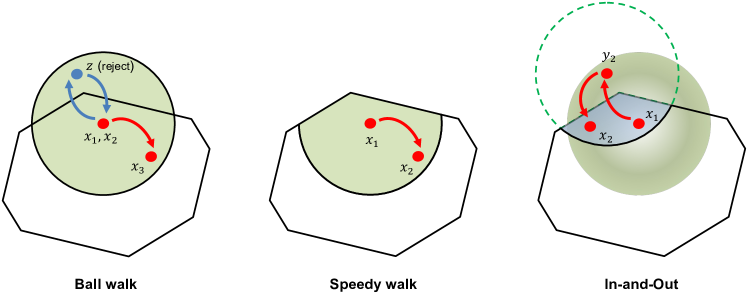
We propose the following 111This name reflects the “geometry” of how the iterates are moving. As we elaborate in Remark 1, the name ‘proximal sampler’ may be more familiar to those from an optimization background. sampler for uniformly sampling from . Each iteration consists of two steps, one that might leave the body and the second accepted only if it is (back) in the body.
Input: initial point , convex body , iterations , threshold , and .
Output: .
It might be illuminating for the reader to compare this algorithm to the well-studied (Algorithm 2); each proposed step is a uniform random point in a fixed-radius ball around the current point, and is accepted only if the proposed point is in the body . In contrast, each iteration of is a two-step process, where the first step (Line 2) ignores the boundary of the body, and the second step (Line 3) is accepted only if a proposal is a feasible point in . We will presently elaborate on the benefits of this variation.
Each successful iteration of the algorithm, i.e., one that is not declared “Failure”, can be called a proper step. We will see that the number of proper steps is directly bounded by isoperimetric constants (such as Poincaré and log-Sobolev) of the target distribution. In fact, this holds quite generally without assuming the convexity of . The implementation of an iteration is based on rejection sampling (Line 3), and our analysis of the efficiency of this step relies crucially on the convexity of . This is reminiscent of the in the literature on convex body sampling (Algorithm 3), which is used as a tool to analyze proper steps of the . We refer the reader to Appendix B for a brief survey on these and related walks.
This simple algorithm can be interpreted as a composition of “flows” in the space of measures. This view will allow us to use tools from stochastic analysis. In particular, we shall demonstrate how to interpret the two steps of one iteration of as alternating forward and backward heat flows.
We begin by defining an augmented probability measure on by
We denote by the marginal distribution of its first component (resp. conditional distribution given the second component), and similarly denote by for the second component. In particular, the marginal in the first component is the uniform distribution over . Sampling from such a joint distribution to obtain the marginal on (say), can be more efficient than directly working only with . This idea was utilized in Gaussian Cooling [CV18] and later as the restricted Gaussian Oracle (RGO) [LST21, Che+22].
Under this notation, Algorithm 1 corresponds to a Gibbs sampling scheme from the two marginals of . To be precise, Line 2 and Line 3 correspond to sampling from
We implement the latter step through rejection sampling; if the number of trials in Line 3 hits the threshold , then we halt and declare failure of the algorithm. It is well known that such a Gibbs sampling procedure will ensure the desired stationarity of .
Stochastic perspective: forward and backward heat flows.
Our algorithm can be viewed through the lens of stochastic analysis, due to an improved analysis for the proximal sampling [Che+22]. This view provides an interpolation in continuous-time, which is simple and powerful. To make this concrete, we borrow an exposition from [Che24, Chapter 8.3]. Let us denote the successive laws of and by and , respectively. Recall that the first step of sampling from (Line 2) yields . This is the result of evolving a probability measure under (forward) heat flow of for some time , given precisely by the following stochastic differential equation: for ,
| () |
where is the standard Brownian process. We write . In particular, for . When , the first step of Algorithm 1 gives
| (1.1) |
The second step of sampling from can be represented by (Line 3). The continuous-time process corresponding to this step might not be obvious. However, let us consider () with . Then, , so the joint distribution of is simply . This implies that . Imagine there is an SDE reversing the forward heat flow in a sense that if we are initialized deterministically at at time , then the law of the SDE at time would be . Then, this SDE would serve as a continuous-time interpolation of the second step.
| Forward flow | Backward flow | |
|---|---|---|
| SDE | ||
| Fokker-Planck |
1.2 Results
Our model of computation is the classical general model for convex bodies [GLS88]. We assume throughout this paper. Below, denotes the -dimensional ball of radius centered at .
Definition 1 (Convex body oracle).
A well-defined membership oracle for a convex body is given by a point , a number , with the guarantee that , and an oracle that correctly answers YES or NO to any query of the form “?”
Definition 2 (Warmness).
A distribution is -warm with respect to another distribution , i.e., for every in the support of , we have .
We now summarize our main result which is further elaborated in Section 3.4 (Theorem 27). Below, is the uniform distribution over , and is the Rényi-divergence of order (see Definition 6).
Theorem 3.
For any given , , and any convex body given by a well-defined membership oracle, there exist choices of parameters such that , starting from an -warm distribution, with probability at least , returns such that . The number of proper steps is , and the expected total number of membership queries is , where is the largest eigenvalue of the covariance of .
We note that for ,
The above guarantee in the Rényi divergence immediately provides , and guarantees as special cases. Previous guarantees for uniformly sampling convex bodies were only in the -distance. For two distributions and , we have
-
1.
for .
-
2.
.
-
3.
(Talagrand’s -inequality) and .
-
4.
[Liu20] and .
The query complexity is better if the convex body is (near-)isotropic, i.e., the uniform distribution over the body has (near-)identity covariance. This relies on recent estimates of the worst-case Poincaré constant for isotropic log-concave distributions [KLS95, Kla23].
Corollary 4.
Assume that is isotropic. Under the same setting as above, succeeds with probability , returning such that . The number of proper steps is , and the expected total number of membership queries is .
Our analysis will in fact show that the bound on the number of proper steps holds for general non-convex bodies and any feasible start in . This is deduced under an -warm start in Corollaries 28 and 29. We remark that such a bound for non-convex uniform sampling is not known for the or the .
Theorem 5.
For any given and set with , with variance and -warm initial distribution achieves after the following number of iterations:
We have two different convergence results above under (8) and (7). Under (8) we have a doubly-logarithmic dependence on the warmness parameter . On the other hand, using (7), which is weaker than (8) (in general, ), the dependence on is logarithmic. We discuss our results further in Section 1.3.
Outline of analysis.
We summarize our proof strategy below, which consists of two steps: (i) The current distribution should converge to the uniform distribution, (ii) within each iteration of the algorithm, the failure probability and the expected number of rejections should be small enough.
-
•
We need to demonstrate that the corresponding Markov chain is rapidly mixing. Here, we use the heat flow perspective to derive mixing rates under any suitable divergence measure (such as , , or ), extending known results for the unconstrained setting [Che+22]. As a result, the mixing analysis reduces to a suitable functional inequality of the target distribution alone.
-
•
We show that the number of rejections in Line 3 over the entire execution of the algorithm is bounded with high probability. To do this, we apply a detailed argument involving local conductance and the convexity of , which relies on techniques from [BNN06]. For this step, we show that with the appropriate choice of variance and threshold , the entire algorithm succeeds with probability . The expected number of rejections is polylogarithmic.
While each individual component resembles pre-existing work in the literature, in their synthesis we will demonstrate how to interleave past developments in theoretical computer science, optimal transport, and functional analysis. The combination of these in this domain yields elegant and surprisingly simple proofs, as well as stronger results.
1.3 Discussion
Here we make a few remarks, contrasting our results with known ones.
No need to be lazy.
Previous uniform samplers like the are made lazy (i.e., with probability , the Markov chain does nothing), to ensure convergence to the target stationary distribution. However, our algorithm does not need this, since we directly show that our sampler contracts towards a uniform distribution.
Unified framework.
We remark that these two different bounds also place the previously known mixing guarantees for in a unified framework. Existing tight guarantees for are in TV distance and based on the log-Sobolev constant, assuming an oracle for implementing each step [LV17]. The known convergence guarantees of (see Appendix B for details), namely the mixing time of for TV distance, are for the composite algorithm [rejection sampling]. Here records only the accepted steps of , so its stationary distribution differs slightly from the uniform distribution (and can be corrected with a post-processing step). On the other hand, actually converges to without any adjustments and achieves stronger Rényi divergence bounds in the same asymptotic complexity. Our analysis shows that the mixing guarantee is determined by isoperimetric constants of the target (Poincaré or log-Sobolev).
Effective step size.
The ’s largest possible step size is of order (see Appendix B) to keep the rejection probability bounded by a constant. This bound could also be viewed as an “effective” step size of . This follows from the fact that the -norm of the Gaussian is concentrated around , and we will set the variance of to , so we have .
What has really changed?
has clear similarities to both and . What then are the changes that allow us to use continuous-time interpolation? One step of is [random step () Metropolis-filter (accept if )]. This filtering is an abrupt discrete step, and it is unclear how to control contraction. It could be replaced by a step of (). Then, each iteration of can be viewed as a Gaussian version of a algorithm.
How can we compare with Iterating speedy steps leads to a biased distribution (one that is proportional to the local conductance). As clarified in Remark 2, one step of (a Gaussian version of) can be understood as a step of backward heat flow. Therefore, if one can control the isoperimetric constants of the biased distribution along the trajectory of the backward flow, then contraction of toward the biased distribution will follow from the simultaneous backward analysis.
2 Preliminaries
Unless otherwise specified, we will use for the -norm on , and operator norm on . We write , to mean that for some universal constant . Similarly, for , while means that simultaneously. We will also use to denote . Lastly, we will use measure and density interchangeably when there is no confusion.
To quantify the convergence rate, we introduce some common divergences between distributions.
Definition 6 (Distance and divergence).
For two measures on , the total variation distance between them is defined by
where is the collection of all measurable subsets of . The -Wasserstein distance is given by
where is the set of all couplings between . Next, we define the -divergence of towards with (i.e., is absolutely continuous with respect to ) as, for some convex function with and ,
The -divergence arises when taking , the -divergence when taking , and the -Rényi divergence is given by
We recall two important functional inequalities of a distribution. We use to denote a probability measure over .
Definition 7.
We say that satisfies a Poincaré inequality (PI) with parameter if for all smooth functions ,
where .
The Poincaré inequality is implied by the log-Sobolev inequality.
Definition 8.
We say that satisfies a log-Sobolev inequality (LSI) with parameter if for all smooth functions ,
where . Equivalently, for any probability measure over with ,
where is the Fisher information of with respect to .
We recall the data-processing inequality for Rényi divergence and -divergence.
Lemma 9 (Data-processing inequality).
For measures , Markov kernel , -divergence , and , it holds that
The aforementioned functional inequalities allow us to show exponential contraction of various divergences, through the following helpful inequality.
Lemma 10 (Grönwall).
Suppose that are two continuous functions, with being differentiable on and satisfying
Then,
3 Analysis
We begin this section by proving some introductory lemmas, which will streamline our later exposition.
We first record two fundamental lemmas, which introduce the mathematical formalism for our analysis. The first is the existence of forward and backward heat flows (Lemma 22), which will interpolate each line in Algorithm 1. These flow equations describe how the laws of and in () and () evolve respectively over time.
Lemma 11.
The forward heat flow equation with initial distribution is given by
and its backward heat flow equation is given by
These admit (weak) solutions on for any initial distribution with .
One successful iteration of is exactly the same as the composition of running the forward heat flow and then backward heat flow, both for time . Its validity is justified in Section 1.1, and we give its proof below.
Lemma 12.
Proof.
We explicitly show that the forward and backward heat flows indeed interpolate the two discrete steps given in Algorithm 1. For the forward part, we have for , so
Regarding the backward part, it is known from [Che+22, Lemma 14] that the construction of the time-reversal SDE ensures that and have the same joint distribution, when (and so ). Hence, , where the last equality follows from . Since we initialize () with , we have
where the last follows from the definition of Line 3. ∎
Our analysis of these objects consists of two parts: (1) demonstrating the mixing of , i.e., how many outer iterations are needed to be sufficiently close to the uniform distribution, and (2) quantifying the failure probability and wasted steps in Line 3.
For (1), we collect in Section 3.1 some important implications of functional inequalities, e.g. the Poincaré and log-Sobolev inequalities, for the uniform distribution. Then in Section 3.2, we exploit the flow perspective of the algorithm to obtain the mixing guarantees. To this end, we revisit the proofs for the contraction results of forward and backward heat flows, and then extend them to our constrained setting:
Theorem 13 (Adapted for uniform distributions, [Che+22]).
Let be the law of the -th output of with initial distribution . Let be the (8) constant of the uniform distribution over . Then, for any ,
For the (7) constant of and any ,
This reduces the problem of obtaining a mixing guarantee to that of demonstrating a functional inequality on the target distribution. For this, it is not strictly necessary that be convex.
On the other hand, convexity of is crucial for the proof of (2). We show in Section 3.3 that the failure probability remains under control by taking a suitable variance and threshold . We then show that the expected number of trials per iteration is of order , not :
Lemma 14 (Per-iteration guarantees).
Let be any convex body in presented by a well-defined membership oracle, the uniform distribution over , and an -warm initial distribution with respect to . For any given and , set , and . Then, the failure probability of one iteration of is at most . Moreover, the expected number of membership queries needed per iteration is .
3.1 Functional inequalities
The contraction of an outer loop of our algorithm is controlled by isoperimetry of the uniform distribution , which is described precisely by a functional inequality. The most natural ones to consider in this setting are the Poincaré inequality (7) and log-Sobolev inequality (8). In Appendix C, we provide a more detailed discussion of how these are related to other important notions of isoperimetry, such as the Cheeger and log-Cheeger inequalities.
Below, we use to denote two arbitrary probability measures over . The relationship between a Poincaré inequality and the -divergence is derived by substituting into (7).
Lemma 15.
Assume that satisfies (7) with parameter . For any probability measure over with , it holds that
The Poincaré inequality implies functional inequalities for the Rényi divergence.
Lemma 16 ([VW19, Lemma 9]).
Assume that satisfies (7) with parameter . For any and probability measure over , it holds that
where is the Rényi Fisher information of order of with respect to .
The log-Sobolev inequality paired with the KL-divergence (8) can be understood as a special case of the following inequality222Such inequalities are often called Polyak-Łojasiewicz inequalities, which say for , and all that for some constant , if . paired with the -Rényi divergence for .
Lemma 17 ([VW19, Lemma 5]).
Assume that satisfies (8) with parameter . For any and probability measure over , it holds that
Note that and .
We have collected below the functional inequalities used to establish the mixing of our algorithm (see Appendix C for a detailed presentation).
Lemma 18.
Let be a convex body with diameter , and be the uniform distribution over . Then, and . If is isotropic, then and .
3.2 Contraction and mixing
We start by analyzing how many outer iterations of are required to be -close to , the uniform distribution over . The contraction of Algorithm 1 comes from analyzing Lines 2 and 3 through the perspective of heat flows (see Section 1.1). To exploit this view, we first revisit the previous contraction analysis in [Che+22], which is carried out for distributions with smooth densities. Although the uniform distribution is not even continuous, we prove a technical lemma (Lemma 22) that enables us to extend previously known results to the uniform distribution. Lastly, combining the previous results with our technical lemma, we obtain clean contraction results of Algorithm 1 toward the uniform distribution in Theorem 23.
Part I: Contraction analysis for smooth distributions.
In this part, we review the contraction results for heat flow and its time-reversal [Che+22], which are intimately connected with our algorithm. We also provide key technical ingredients needed for its proof, such as the computations for measures evolving under simultaneous forward/backward heat flows. We refer interested readers to Appendix D for additional details. Only in Part I, we assume that denotes a probability measure with smooth density.
Forward heat flow.
We begin by introducing the “heat flow” equation (or also known as the Fokker-Planck equation), which describes the evolution of the law of under (),
| () |
It is well known that one can realize this equation in discrete time through a Gaussian transition density, in the sense that, for (the solution at time to () with initial condition ), and for any smooth function ,
where .333 is often called the heat semigroup. By this we can formally identify , and also write for the law of , where solves ().
Backward heat flow.
Although there are many ways to define a “reversal” of , we will use the notion of adjoint introduced by [KP21], which is the most immediately useful.
Given some initial measure and some time horizon , the adjoint corresponds to reversing () for times in when the initial distribution under consideration is . For other measures, it must be interpreted more carefully, and is given by the following partial differential equation starting from some measure (see (D.1) and its derivation):
| () |
Write , where is a family of transition densities. Write for the joint distribution of the -marginals of (), when , and for the conditional. Note that . It is also known that () gives a time-reversal of the heat equation at the SDE level, in the sense that we can interpret . Thus , and for all .
The ultimate purpose of this machinery is to affirm our earlier description of the Gibbs sampling procedure as alternating forward and backward heat flows. Indeed, notice that, if is the law of the iterate at some iteration , then is precisely under our scheme, while is , assuming is well defined for non-smooth measures . Thus, while Algorithm 1 is implemented via discrete steps, it can be exactly analyzed through arguments in continuous time. We shall see the benefits of this shortly.
Instead of considering the change in metrics along the evolution of with respect to “fixed” , it will be useful to consider the simultaneous evolution of (and similarly ). This type of computation was carried out for specific metrics in earlier work [VW19, Che+22]. The following is a more generalized form of one appearing in [Yua+23, Lemma 2]. In the lemma below, we consider an arbitrary diffusion equation with corresponding Fokker-Planck equation:
| (3.1) |
where is smooth, , and if .
Lemma 19 (Decay along forward/backward heat flows).
Let denote the laws of the solutions to (3.1) starting at respectively. Then, for any differentiable function ,
Proof.
The case where is an application of the chain rule, so it suffices to take and simply differentiate an -divergence.
For brevity, we drop the variable of functions involved, and proceed as follows:
where in we substitute the F-P equation from (3.1). Integrating by parts (i.e., for a real-valued function and vector-valued function ), we have that
| (3.2) |
On the other hand, we have that
The second term cancels with the RHS of (3.2). We have a similar cancellation for the term:
and
Combining these, we are left with
Finally, we note that
Putting it all together, noticing that the drift terms cancel, we are left with
which completes the proof. ∎
To recover the decay result for the -Rényi divergence, one can substitute and . For the -divergence, instead substitute and . From this, we can obtain a single step of decay for the Rényi and -divergences under different functional inequalities.
Lemma 20 (Functional inequalities under Gaussian convolutions, [Cha04, Corollary 13]).
The following inequality holds for any with finite log-Sobolev and Poincaré constants,
Combining the previous two lemmas, we can establish contraction between and after one forward/backward iteration.
Theorem 21 ([Che+22, Theorem 3 and 4]).
Assume , a measure with smooth density, satisfies (8) with constant . For any and initial distribution with a smooth density, denoting again ,
Proof.
Since the SDE in (3.1) captures the forward heat flow (), we set and in Lemma 19 to and , respectively, obtaining contraction along the forward heat flow as follows: Substituting the -Rényi into Lemma 19, we have, from the definition of the Rényi divergence as with and ,
where in , we use again that , and uses that , and the last equality recalls the definition of the Rényi Fisher information. This yields
where we used Lemma 17 in and Lemma 20 in . Applying Grönwall’s inequality (Lemma 10),
Since the SDE (3.1) also captures the backward equation (), we set and in Lemma 19 to and respectively, obtaining contraction along the backward heat flow:
where follows from that and due to Lemma 20. Applying Lemma 10 again yields
Composing these two inequalities leads to the decay rate claimed in the theorem.
The result in the -divergence can be derived entirely analogously. For instance, the decay from the forward part can be shown as follows:
where follows from Lemma 15. Applying Grönwall’s inequality then gives
The decay along the backward heat flow in is entirely analogous to the Rényi case. Then we combine two contraction results from the forward and backward flows, completing the proof.
Part II: Extension to constrained distributions.
We now prove a technical lemma that extends the contraction results to constrained distributions. This lemma guarantees the existence of weak solutions to two stochastic processes that describe the evolution of distributions involved in Line 2 and 3 in , in addition to lower-semicontinuity of -divergence. We shall prove it for any measure that is absolutely continuous with respect to , since this imposes no additional technical hurdles.
Lemma 22.
Let be a measure, absolutely continuous with respect to the uniform measure . The forward and backward heat flow equations given by
admit solutions on , and the weak limit exists for any initial measure with bounded support. Moreover, for any -divergence with lower semi-continuous,
Proof.
The existence of weak solutions for the forward equation is well-known, since can be weakly approximated by measures with continuous density, for which the heat equation admits a unique solution for all time. In particular, the weak solution is for .
The reverse SDE is more subtle, since will in general cease to be Lipschitz as . On the other hand, for any , we can write explicitly
If one considers the system started at and solve the forward-backward Fokker-Planck equations on times , then and
This follows from that if we consider system started at time , with initial distribution , then we obtain the above through the Bayesian perspective on the forward and reverse heat semigroups, elaborated in Appendix D.
We now show that the following integral is indeed integrable, so is well-defined:
For fixed and ,
as the support of is constrained to . Since has bounded support, for some constant . Thus,
and the last bound is integrable in .
We then show the pointwise convergence of to as . Note that , as has a bounded support. Also, the denominator is independent of due to
Hence, for ,
As shown above, the last bound is integrable with respect to , so the dominated convergence theorem implies
Thus, the pointwise convergence follows. Note that if we take , then is the distribution of the backwards step of our algorithm. In particular, this corresponds to first sampling , then , which is precisely the law of given by ().
In the sequel, we will only consider . Since the Rényi divergence is a continuous function of the divergence (see Definition 6), which itself is an -divergence, it enjoys the same lower-semicontinuity properties. Using this lower-semicontinuity together with the decay results in Theorem 21, we can easily derive the contraction results of in and for any . We remark that this result does not require convexity of .
Theorem 23.
Let be the law of the -th output of with initial distribution . Let be the (8) constant of the uniform distribution over . Then, for any ,
Proof.
Let us set and . Then, , , and , . For small , as is -smooth, we can now invoke the decay results with step size in Theorem 21. Thus, for contraction constants and respectively when and ,
where we used the data-processing inequality for the last inequality. By the second result of Lemma 22, sending leads to
Repeating this argument times completes the proof. ∎
3.3 Failure probability and wasted steps
We begin by defining a suitable version of local conductance [KLS97].
Definition 24 (Local conductance).
The local conductance on is defined by
The local conductance at quantifies the success probability of the proposal at in Line 3. Then the expected number of trials until the first success of Line 3 is . Revisiting (1.1), we can notice .
Naïve analysis for expected number of trials.
Starting from , when we just naïvely sample from for all without imposing any failure condition, the expected number of trials for one iteration is that for the probability density of ,
This suggests that one should consider the algorithm as having “failed” if the number of trials exceeds some threshold.
Refined analysis under a failure condition.
Going forward, we assume an -warm start as in previous work for uniform sampling algorithms. By induction we have for all .
Lemma 25 (Propagation of warm-start).
From an -warm start, we have for all .
Proof.
Assume that satisfies the -warm start. Then, for any measurable and the transition kernel of Algorithm 1 at ,
where the last equality follows from the stationarity of . Hence, . ∎
We now establish a lemma that comes in handy when analyzing the failure probability of the algorithm. In essence, this lemma bounds the probability that taking a Gaussian step from in Line 2 gets -distance away from . Let us denote the -blowup of by .
Lemma 26.
for and variance , where is some constant and .
Proof.
For , we can take the supporting half-space at containing , due to convexity of . Then,
| (3.3) |
Let us denote the tail probability of the -dimensional Gaussian with variance by
By the co-area formula and integration by parts,
| (3.4) |
Recall that for due to a standard tail bound on a Gaussian distribution. This tail bound, combined with
ensures that vanishes at . Hence, bounding the first term in (3.4) by results in
where in we used the tail bound of a Gaussian, and follows from that in the regime of , we have for . Putting the last bound into (3.3) completes the proof of the claim. ∎
Now we choose a suitable threshold for bounding the failure probability. Following (3.3) in the proof, one can notice that for , , and ,
Thus, the expected number of trials from for the rejection sampling in Line 3 is . Intuitively, one can ignore whatever happens in , since takes up most of measure of . As the number of trials from is at least in expectation, the most straightforward way to ignore algorithmic behaviors from is simply to set the threshold to . Even though the threshold is , the expected number of trials is much lower.
Lemma 14 bounds the failure probability and expected number of trials per iteration.
Proof of Lemma 14.
For , the failure probability is . Since implies , it follows that
Then,
where we used . Taking , , and , we can bound the last line by . Therefore,
We now bound the expected number of trials per iteration. Let be the minimum of the threshold and the number of trials until the first success. Then the expected number of trials per step is bounded by due to . Thus,
Therefore, the expected number of trials per step is , and the claim follows since each trial uses one query to the membership oracle of . ∎
3.4 Putting it together
We can now show that subsumes previous results on uniform sampling from convex bodies (such as and ), providing detailed versions of the main results in Section 1.2.
We first establish that the query complexity of matches that of the under stronger divergences. Recall that .
Theorem 27.
For any given , , defined below and any convex body given by a well-defined membership oracle, consider (Algorithm 1) with an -warm initial distribution , , and . For the uniform distribution over ,
-
•
It achieves after iterations. With probability , the algorithm iterates this many times without failure, using expected number of membership queries in total.
-
•
For isotropic , with probability , the algorithm achieves with iterations, using membership queries in expectation.
Proof.
We just put together Lemma 14 and Theorem 23. For target accuracy , we use the -decay under (7) for in Theorem 23. The -warm start assumption guarantees . Due to (Lemma 18), can achieve after iterations. Since each iteration has -failure probability by Lemma 14, the union bound ensures that the total failure probability is at most throughout iterations. Lastly, each iteration requires membership queries in expectation by Lemma 14. Therefore, uses expected number of membership queries over iterations. Since is non-decreasing in , we can obtain the desired bound on for .
For isotropic , we have , so the claim immediately follows from (see Lemma 18). ∎
We now show that the number of proper steps is bounded as claimed for general non-convex bodies and any feasible start in . We first establish this result under an -warm start (Theorem 5).
Proof of Theorem 5..
For , we use the decay result under (7). In this case, decays under two different rates depending on the value of . It first needs iterations until reaches . Then, additionally needs iterations, and thus it needs iterations in total. By substituting , we complete the proof. ∎
Next, we show that mixes from any start.
Corollary 28.
For any given and set , with variance and any feasible start achieves after iterations.
Proof.
We then obtain the following corollary for a convex body .
Corollary 29.
For any given and convex body , with variance and an -warm initial distribution achieves after iterations. If is isotropic, then only needs iterations.
Proof.
For convex , it follows from Lemma 18 that and for isotropic . The rest of the proof can be completed in a similar way. ∎
For , requires iterations and in particular iteration for isotropic uniform distributions. These results match those of [KLM06, LV17] (see Theorem 31).
Acknowledgements.
We are deeply grateful to Andre Wibisono and Sinho Chewi for helpful comments and pointers to the literature for Lemma 19. This work was supported in part by NSF award 210644, NSERC through the CGS-D award, and a Simons Investigator award.
pages14 rangepages10 rangepages39 rangepages-1 rangepages24 rangepages27 rangepages39 rangepages1 rangepages31 rangepages28 rangepages28 rangepages37 rangepages12 rangepages21 rangepages46 rangepages17 rangepages38 rangepages49 rangepages92 rangepages41 rangepages3 rangepages14 rangepages11 rangepages30 rangepages19 rangepages50 rangepages20 rangepages26 rangepages13 rangepages66 rangepages9 rangepages58 rangepages7 rangepages10 rangepages17 rangepages15 rangepages25 rangepages16 rangepages19 rangepages9 rangepages54 rangepages21 rangepages10 rangepages43 rangepages13 rangepages13 rangepages7 rangepages1 rangepages27 rangepages28
References
- [AC21] Kwangjun Ahn and Sinho Chewi “Efficient constrained sampling via the mirror-Langevin algorithm” In Advances in Neural Information Processing Systems (NeurIPS) 34, 2021, pp. 28405–28418
- [AFP00] Luigi Ambrosio, Nicola Fusco and Diego Pallara “Functions of bounded variation and free discontinuity problems” Oxford University Press, 2000
- [AGS05] Luigi Ambrosio, Nicola Gigli and Giuseppe Savaré “Gradient flows: in metric spaces and in the space of probability measures” Springer Science & Business Media, 2005
- [BNN06] Mikhail Belkin, Hariharan Narayanan and Partha Niyogi “Heat flow and a faster algorithm to compute the surface area of a convex body” In Foundations of Computer Science (FOCS), 2006, pp. 47–56 IEEE
- [Bes+95] Julian Besag, Peter Green, David Higdon and Kerrie Mengersen “Bayesian computation and stochastic systems” In Statistical Science JSTOR, 1995, pp. 3–41
- [Bil95] Patrick Billingsley “Probability and measure” John Wiley & Sons, 1995
- [Bin+19] Eli Bingham et al. “Pyro: Deep universal probabilistic programming” In The Journal of Machine Learning Research (JMLR) 20, 2019, pp. 28:1–28:6
- [Bro+17] Nicolas Brosse, Alain Durmus, Ãric Moulines and Marcelo Pereyra “Sampling from a log-concave distribution with compact support with proximal Langevin Monte Carlo” In Conference on Learning Theory (COLT) 65 PMLR, 2017, pp. 319–342
- [BEL15] Sebastien Bubeck, Ronen Eldan and Joseph Lehec “Finite-time analysis of projected Langevin Monte Carlo” In Advances in Neural Information Processing Systems (NeurIPS) 28, 2015
- [BEL18] Sébastien Bubeck, Ronen Eldan and Joseph Lehec “Sampling from a log-concave distribution with projected Langevin Monte Carlo” In Discrete & Computational Geometry (DCG) 59 Springer, 2018, pp. 757–783
- [Cha04] Djalil Chafaï “Entropies, convexity, and functional inequalities, On Phi-entropies and Phi-Sobolev inequalities” In Journal of Mathematics of Kyoto University 44.2 Duke University Press, 2004, pp. 325–363
- [Che70] Jeff Cheeger “A lower bound for the smallest eigenvalue of the Laplacian” In Problems in analysis 625.195-199 Princeton UP, 1970, pp. 110
- [Che+22] Yongxin Chen, Sinho Chewi, Adil Salim and Andre Wibisono “Improved analysis for a proximal algorithm for sampling” In Conference on Learning Theory (COLT), 2022, pp. 2984–3014 PMLR
- [Che21] Yuansi Chen “An almost constant lower bound of the isoperimetric coefficient in the KLS conjecture” In Geometric and Functional Analysis (GAFA) 31 Springer, 2021, pp. 34–61
- [Che24] Sinho Chewi “Log-concave sampling” Book draft available at https://chewisinho.github.io, 2024
- [CV16] Ben Cousins and Santosh S Vempala “A practical volume algorithm” In Mathematical Programming Computation 8.2 Springer, 2016, pp. 133–160
- [CV18] Ben Cousins and Santosh S Vempala “Gaussian Cooling and algorithms for volume and Gaussian volume” In SIAM Journal on Computing (SICOMP) 47.3 SIAM, 2018, pp. 1237–1273
- [Dal17] Arnak Dalalyan “Further and stronger analogy between sampling and optimization: Langevin Monte Carlo and gradient descent” In Conference on Learning Theory (COLT), 2017, pp. 678–689 PMLR
- [DT12] Arnak S Dalalyan and Alexandre B Tsybakov “Sparse regression learning by aggregation and Langevin Monte-Carlo” In Journal of Computer and System Sciences 78.5 Elsevier, 2012, pp. 1423–1443
- [DMM19] Alain Durmus, Szymon Majewski and Blazej Miasojedow “Analysis of Langevin Monte Carlo via convex optimization” In The Journal of Machine Learning Research (JMLR) 20.1 JMLR. org, 2019, pp. 2666–2711
- [DFK91] Martin Dyer, Alan Frieze and Ravi Kannan “A random polynomial-time algorithm for approximating the volume of convex bodies” In Journal of the ACM (JACM) 38.1 ACM New York, NY, USA, 1991, pp. 1–17
- [Eld13] Ronen Eldan “Thin shell implies spectral gap up to polylog via a stochastic localization scheme” In Geometric and Functional Analysis (GAFA) 23.2 Springer, 2013, pp. 532–569
- [FYC23] Jiaojiao Fan, Bo Yuan and Yongxin Chen “Improved dimension dependence of a proximal algorithm for sampling” In Conference on Learning Theory (COLT), 2023, pp. 1473–1521 PMLR
- [GKV23] Khashayar Gatmiry, Jonathan Kelner and Santosh S Vempala “Sampling with barriers: Faster mixing via Lewis weights” In arXiv preprint arXiv:2303.00480, 2023
- [GC11] Mark Girolami and Ben Calderhead “Riemann manifold Langevin and Hamiltonian Monte Carlo methods” In Journal of the Royal Statistical Society: Series B (Statistical Methodology) 73.2 Wiley Online Library, 2011, pp. 123–214
- [Gop+23] Sivakanth Gopi et al. “Algorithmic aspects of the Log-Laplace transform and a non-Euclidean proximal sampler” In Conference on Learning Theory (COLT) 195 PMLR, 2023, pp. 2399–2439
- [GLS88] Martin Grötschel, László Lovász and Alexander Schrijver “Geometric algorithms and combinatorial optimization” Springer, 1988
- [GHZ22] Mert Gürbüzbalaban, Yuanhan Hu and Lingjiong Zhu “Penalized Langevin and Hamiltonian Monte Carlo algorithms for constrained sampling” In arXiv preprint arXiv:2212.00570, 2022
- [Har+17] Hulda S Haraldsdóttir et al. “CHRR: coordinate hit-and-run with rounding for uniform sampling of constraint-based models” In Bioinformatics 33.11 Oxford University Press, 2017, pp. 1741–1743
- [Jia+21] He Jia, Aditi Laddha, Yin Tat Lee and Santosh S Vempala “Reducing isotropy and volume to KLS: an volume algorithm” In Symposium on Theory of Computing (STOC), 2021, pp. 961–974
- [Jia21] Qijia Jiang “Mirror Langevin Monte Carlo: the case under isoperimetry” In Advances in Neural Information Processing Systems (NeurIPS) 34, 2021, pp. 715–725
- [KLM06] Ravi Kannan, László Lovász and Ravi Montenegro “Blocking conductance and mixing in random walks” In Combinatorics, Probability and Computing 15.4 Cambridge University Press, 2006, pp. 541–570
- [KLS95] Ravi Kannan, László Lovász and Miklós Simonovits “Isoperimetric problems for convex bodies and a localization lemma” In Discrete & Computational Geometry 13.3 Springer, 1995, pp. 541–559
- [KLS97] Ravi Kannan, László Lovász and Miklós Simonovits “Random walks and an volume algorithm for convex bodies” In Random Structures & Algorithms (RS&A) 11.1 Wiley Online Library, 1997, pp. 1–50
- [KN12] Ravindran Kannan and Hariharan Narayanan “Random walks on polytopes and an affine interior point method for linear programming” In Mathematics of Operations Research 37.1 INFORMS, 2012, pp. 1–20
- [KP21] Bo’az Klartag and Eli Putterman “Spectral monotonicity under Gaussian convolution” In arXiv preprint arXiv:2107.09496, 2021
- [Kla23] Boáz Klartag “Logarithmic bounds for isoperimetry and slices of convex sets” In Ars Inveniendi Analytica Ars Inveniendi, 2023
- [KL22] Boáz Klartag and Joseph Lehec “Bourgain’s slicing problem and KLS isoperimetry up to polylog” In Geometric and Functional Analysis (GAFA) 32.5 Springer, 2022, pp. 1134–1159
- [Koo+22] Yunbum Kook, Yin Tat Lee, Ruoqi Shen and Santosh S Vempala “Sampling with Riemannian Hamiltonian Monte Carlo in a constrained space” In Advances in Neural Information Processing Systems (NeurIPS) 35, 2022, pp. 31684–31696
- [Koo+23] Yunbum Kook, Yin Tat Lee, Ruoqi Shen and Santosh S Vempala “Condition-number-independent convergence rate of Riemannian Hamiltonian Monte Carlo with numerical integrators” In Conference on Learning Theory (COLT) 195 PMLR, 2023, pp. 4504–4569
- [KV23] Yunbum Kook and Santosh S Vempala “Gaussian Cooling and Dikin walks: The Interior-Point Method for logconcave sampling” In arXiv preprint arXiv:2307.12943, 2023
- [Led94] Michel Ledoux “A simple analytic proof of an inequality by P. Buser” In Proceedings of the American Mathematical Society 121.3, 1994, pp. 951–959
- [LST21] Yin Tat Lee, Ruoqi Shen and Kevin Tian “Structured logconcave sampling with a restricted Gaussian oracle” In Conference on Learning Theory (COLT), 2021, pp. 2993–3050 PMLR
- [LV18] Yin Tat Lee and Santosh S Vempala “Convergence rate of Riemannian Hamiltonian Monte Carlo and faster polytope volume computation” In Symposium on Theory of Computing (STOC), 2018, pp. 1115–1121
- [LV17] Yin Tat Lee and Santosh Srinivas Vempala “Eldan’s stochastic localization and the KLS hyperplane conjecture: An improved lower bound for expansion” In Foundations of Computer Science (FOCS), 2017, pp. 998–1007 IEEE
- [Leh23] Joseph Lehec “The Langevin Monte Carlo algorithm in the non-smooth log-concave case” In The Annals of Applied Probability 33.6A Institute of Mathematical Statistics, 2023, pp. 4858–4874
- [LNP12] Nathan E Lewis, Harish Nagarajan and Bernhard O Palsson “Constraining the metabolic genotype–phenotype relationship using a phylogeny of in silico methods” In Nature Reviews Microbiology 10.4 Nature Publishing Group, 2012, pp. 291–305
- [Li+22] Ruilin Li, Molei Tao, Santosh S Vempala and Andre Wibisono “The mirror Langevin algorithm converges with vanishing bias” In International Conference on Algorithmic Learning Theory (ALT), 2022, pp. 718–742 PMLR
- [Liu20] Yuan Liu “The Poincaré inequality and quadratic transportation-variance inequalities” In Electronic Journal of Probability 25.1, 2020, pp. 1–16
- [Lov99] László Lovász “Hit-and-run mixes fast” In Mathematical Programming 86 Springer, 1999, pp. 443–461
- [LS90] László Lovász and Miklós Simonovits “The mixing rate of Markov chains, an isoperimetric inequality, and computing the volume” In Foundations of Computer Science (FOCS), 1990, pp. 346–354 IEEE
- [LS93] László Lovász and Miklós Simonovits “Random walks in a convex body and an improved volume algorithm” In Random Structures & Algorithms (RS&A) 4.4 Wiley Online Library, 1993, pp. 359–412
- [LV03] László Lovász and Santosh S Vempala “Hit-and-run is fast and fun” In preprint, Microsoft Research, 2003
- [LV06] László Lovász and Santosh S Vempala “Hit-and-run from a corner” In SIAM Journal on Computing (SICOMP) 35.4 SIAM, 2006, pp. 985–1005
- [MT07] Frank McSherry and Kunal Talwar “Mechanism design via differential privacy” In Foundations of Computer Science (FOCS), 2007, pp. 94–103 IEEE
- [Mil09] Emanuel Milman “On the role of convexity in isoperimetry, spectral gap and concentration” In Inventiones Mathematicae 177.1 Springer, 2009, pp. 1–43
- [Mir17] Ilya Mironov “Rényi differential privacy” In Computer Security Foundations Symposium (CSF), 2017, pp. 263–275 IEEE
- [Smi84] Robert L Smith “Efficient Monte Carlo procedures for generating points uniformly distributed over bounded regions” In Operations Research 32.6 INFORMS, 1984, pp. 1296–1308
- [SWW23] Vishwak Srinivasan, Andre Wibisono and Ashia Wilson “Fast sampling from constrained spaces using the Metropolis-adjusted mirror Langevin algorithm” In arXiv preprint arXiv:2312.08823, 2023
- [Sta20] Stan Development Team “RStan: the R interface to Stan” R package version 2.21.2, 2020 URL: http://mc-stan.org/
- [Thi+13] Ines Thiele et al. “A community-driven global reconstruction of human metabolism” In Nature Biotechnology 31.5 Nature Publishing Group, 2013, pp. 419–425
- [Vem05] Santosh S Vempala “Geometric random walks: a survey” In Combinatorial and Computational Geometry 52.573-612 Cambridge University Press Cambridge, 2005, pp. 2
- [VW19] Santosh S Vempala and Andre Wibisono “Rapid convergence of the unadjusted Langevin algorithm: Isoperimetry suffices” In Advances in Neural Information Processing Systems (NeurIPS) 32, 2019
- [Vil09] Cédric Villani “Optimal transport: old and new” Springer, 2009
- [Yua+23] Bo Yuan et al. “On a class of Gibbs sampling over networks” In Conference on Learning Theory (COLT), 2023, pp. 5754–5780 PMLR
- [Zha+20] Kelvin Shuangjian Zhang, Gabriel Peyré, Jalal Fadili and Marcelo Pereyra “Wasserstein control of mirror Langevin Monte Carlo” In Conference on Learning Theory (COLT), 2020, pp. 3814–3841 PMLR
Appendix A Related work
Sampling from constrained log-concave distributions is a fundamental task arising in many fields. Uniform sampling with convex constraints is its simplest manifestation, which was first studied as a core subroutine for a randomized volume-computation algorithm [DFK91]. Since then, this fundamental problem has been studied for over three decades [LS90, LS93, KLS97, LV03, LV06, BEL18, Bro+17]. We review these algorithms, grouping them under three categories — geometric random walks, structured samplers, and diffusion-type samplers. Below, is convex.
Geometric random walk.
is a simple metropolized random walk; it draws uniformly at random from a ball of radius centered at a current point , and moves to if and stays at otherwise. In the literature, actually refers to a composite algorithm consisting of [ rejection sampling], where records only the accepted steps of (see Appendix B for details). The step size should be set to to avoid stepping outside of . [KLS97] showed that needs membership queries to be -close to in , where is the diameter of , and the warmness parameter measures the closeness of the initial distribution to the target uniform distribution .
is another zeroth-order algorithm that needs no step size; it picks a uniform random line passing a current point, and move to a uniform random point on . [LV06] shows that, if we define the second moment as , then requires queries. Notably, this algorithm has a poly-logarithmic dependence on as opposed to .
Both algorithm are affected by skewed shape of (i.e., large or ), so these samplers are combined with pre-processing step called rounding. This procedure finds a linear transformation that makes the geometry of less skewed and so more amenable to sampling. In literature, there exists a randomized algorithm [Jia+21] that rounds and generates a good warm start (i.e., ), with used as a core subroutine. This algorithm takes up queries in total, and in such position with the good warm start, only needs queries to sample from .
Structured samplers.
The aforementioned samplers based on geometric random walks require only access to the membership oracle of the convex body without any additional structural assumptions. The alternate paradigm of geometry-aware sampling attempts to exploit the structure of convex constraints, with the aim of expediting the convergence of the resultant sampling schemes. One common assumption is to make available a self-concordant barrier function which has regularity on its high-order derivatives and blows up when approaching the boundary . The Hessian of encodes the local geometry of the constraint, and the samplers often work directly with .
The first canonical example of such a zeroth-order sampler is used when is given by linear constraints [KN12]; it draws a uniform sample from an ellipsoid (characterized by ) of fixed radius around a current point, and is often combined with a Metropolis adjustment. [KN12] shows that mixes in steps, although each iteration is slightly more expensive than one membership query. This algorithm requires no rounding, but still needs a good warm-start, which can be achieved by an annealing-type algorithm using iterations of [KV23].
is a structured sampler that exploits the first-order information of the potential (i.e., ) [GC11]; its proposal is given as the solution to the Hamilton’s ODE equation, followed by the Metropolis-filter. In the linear-constraint setting above, this sampler requires many iterations to achieve -close distance to [LV18]. This sampler is further analyzed for practical ODE solvers [Koo+23] and for more sophisticated self-concordant barriers [GKV23].
Similarly, [Zha+20, Jia21, AC21, Li+22] is a class of algorithms which converts the constrained problem into an unconstrained one obtained by considering the pushforward of the constrained space by . The algorithm can also be metropolized [SWW23]. The best known rates for this algorithm are under some strong assumptions on .
Diffusion-type samplers.
Samplers based on discretizations of Itô diffusions, stochastic processes which rapidly mix to in continuous time, have long been used for sampling without constraints [Bes+95, DT12, Dal17, Che24]. While the underlying stochastic processes generalize easily to constrained settings, the discretization analysis relies crucially on the smoothness of the target distribution. This is clearly impossible to achieve in the constrained setting, and so some techniques are required to circumvent this difficulty. These algorithms, however, generalize easily to the more general problem of sampling from distributions of the form , by naturally incorporating first order information from .
The first approach for adapting diffusion-based samplers [BEL15, BEL18, Leh23] iterates a two-step procedure. First, a random step is taken, with for some appropriately chosen step ,444A gradient step can be added in the more general case, for sampling from and then project it to , i.e., . The complexity is given in terms of queries to a projection oracle, each call to which can be implemented with a polynomial number of membership oracle queries; a total of queries are needed to be -close in to . Another approach, which uses an algorithmically designed “soft” penalty instead of a projection, was proposed in [GHZ22], and achieves a rate estimate of .
A second approach, suggested by [Bro+17], considers a different proximal scheme, which performs a “soft projection” onto , by taking steps like . It is called Moreau-Yosida regularized Langevin, named after an analogous regularization scheme for constrained optimization. This scheme also relies on access to a projection oracle for , and quantifies their query complexity accordingly. Their final rate estimate is to be -close in distance to .
Observing the prior work integrating diffusion-based sampling with convex constraints, the dependence on the key parameters , while polynomial, are many orders worse than the rates for zeroth-order samplers such as . In contrast, our analysis not only recovers but in some sense surpasses the known rates for , while harmonizing well with the continuous-time perspective of diffusions.
Proximal schemes for sampling.
The Gibbs sampling scheme used in this paper was inspired by the restricted Gaussian oracle introduced in [LST21] (in turn inspired by Gaussian Cooling [CV18]), which alternately iterates between a pure Gaussian step, and a “proximal” step (which we elaborate in our exposition). This scheme was given novel interpretations by [Che+22], which showed that it interpolates the forward and backward heat flows, in the sense defined by [KP21]. The backward heat flow itself is intimately related to stochastic localization schemes, invented and popularized in [Eld13, Che21].
This formulation proved surprisingly powerful, allowing many existing rates in unconstrained sampling to be recovered from a relatively simple analysis. This was further extended by [FYC23] to achieve the current state-of-the-art rate in unconstrained sampling. Finally, [Gop+23] suggest that this could be applied to tackle some constrained problems. However, the assumptions in this final mentioned work are not compatible with the uniform sampling problem on general convex bodies.
Appendix B and
We restate the previously known guarantees for uniform sampling by and . Below, let denote the -dimensional ball of radius centered at .
Input: initial distribution , convex body , iterations , step size .
is particularly simple; draw a uniform random point from around the current point, and go there if the drawn point is inside of and stay at the current point otherwise. Its stationary distribution can be easily seen to be , the uniform distribution over .
In the literature, there are two approaches to analyzing the convergence rate of this sampler: (i) a direct analysis via the -conductance of and (ii) an indirect approach which first passes through .
Direct analysis.
The following -guarantee is obtained by lower bounding the -conductance of , which requires a one-step coupling argument and the Cheeger inequality for . We refer interested readers to [Vem05, Section 5].
Theorem 30 (Convergence of ).
For any and convex body presented by a well-defined membership oracle, let be the distribution after steps of with an -warm initial distribution . Then, with step size achieves for . If is isotropic, then only needs iterations.
The mixing time of under this approach has a polynomial dependence on , rather than a polylogarithmic dependence.
Indirect analysis through .
[KLS97] introduced , which could be viewed as a version of and converges to a speedy distribution (see Proposition 1), which is slightly biased from . Then, is used together with another algorithmic component (rejection sampling) [KLS97, Algorithm 4.15] that converts the speedy distribution to the uniform distribution. In the literature, often refers to ‘ combined with the conversion step’, rather than a direct implementation of Algorithm 2. Strictly speaking, a mixing guarantee of this combined algorithm should not be referred to as a provable guarantee of .
Input: initial distribution , convex body , iterations , step size .
As opposed to , always takes some step at each iteration. However, the problem of sampling from in Line 3 is not straightforward. This step admits the following implementation based on rejection sampling, via a procedure denoted by :
-
•
Propose .
-
•
Set if . Otherwise, repeat the proposal.
Each actual step (indexed by ) in is called a proper step, and rejected steps during are called improper steps. For example, if are the positions produced by , then only proper steps are recorded by .
To describe the theoretical guarantees of , we define the local conductance at , which measures the success probability of the rejection sampling scheme in :
and define the average conductance:
Proposition 1 ([KLS97]).
The stationary distribution of has density
The speedy distribution is indeed different from the uniform distribution , and this discrepancy is quantified in terms of the average conductance.
Proposition 2 ([KLS97, Page 22]).
.
One can relate the step size to the average conductance.
Proposition 3 (Bound on average conductance, [KLS97, Corollary 4.5]).
.
The best known result for ’s mixing is due to [KLM06] devising the blocking conductance and using the log-Cheeger inequality. When is isotropic (i.e., it has covariance proportional to the identity matrix), [LV17] improves the mixing bound via the log-Cheeger constant.
Theorem 31 (Mixing of ).
For any and convex body presented by a well-defined membership oracle, let be the distribution after proper steps of started at any feasible point . Then, with step size achieves for . From an -warm start, the expected number of improper steps during iterations is . When is isotropic, needs proper steps to achieve - distance to .
Then, [KLS97] uses the following post-processing step to obtain an approximately uniform distribution on , with a provable guarantee.
: Call to obtain a sample until . If so, return .
Proposition 4 ([KLS97, Theorem 4.16]).
Under the same setting above, assume for step size and fixed . For given by , it holds that , and the expected number of calls on the conversion algorithm is at most .
Combining the previous two results, we conclude that the total expected number of membership queries to obtain a sample -close to in is , which now has a poly-logarithmic dependence on .
Remark 2 (Backward heat flow analysis of ).
Consider a Gaussian version of , whose one-step corresponds to , and this transition kernel exactly matches integrating () for time . Thus, due to the stationarity of under , where is the transition kernel defined by the backward heat flow for time that reverses to . Hence, if we can control the LSI/PI constants of along the backward heat-flow’s trajectory, then we could directly analyze by emulating computations in Lemma 21.
Appendix C Functional inequalities
We provide full details on functional inequalities omitted in Section 3.1. We use and to denote a probability measure and log-concave probability measure over , respectively.
Cheeger and PI constants.
The Cheeger isoperimetric constant measures how large surface area a measurable subset with larger volume has, defined by
where the infimum is taken over all measurable subsets , and is the Minkowski content of under defined as, for ,
[Che70] established 555The opposite direction also holds for log-concave distributions due to [Mil09], while for general distributions due to [Led94]., and then [KLS95] showed that for covariance matrix ,
| (C.1) |
This immediately leads to for the uniform distribution over a convex body with diameter .
Kannan et al. proposed the KLS conjecture in the same paper, which says that for the spectral norm ,
While the original result in [KLS95] ensures for an isotropic log-concave distribution (due to ), this conjecture indeed claims for such case. Following a line of work [LV17, Che21, KL22, Kla23], the current bound is
which implies that when is isotropic for convex .
Log-Cheeger and LSI constants.
Just as the Cheeger and PI constants are related above, there are known connections between LSI and log-Cheeger constants. The log-Cheeger constant of a distribution is defined as
[Led94] established that 666The opposite direction holds under dimension-scaling due to [Led94]: ., and [KLM06] showed that any log-concave distributions with support of diameter satisfy . Later in 2016, [LV17] improved this to under isotropy. Therefore, for convex , it follows that and that if is isotropic.
Appendix D The Wasserstein geometry
We present additional technical background on the Wasserstein geometry and Markov semigroup theory. Interested readers can refer to [Vil09, AGS05, Che24] for standard references on Wasserstein spaces and applications to sampling.
Wasserstein gradient.
Let be the space of probability measures admitting densities on with finite second moment. Although there are many ways to metrize , the geometry induced by the Wasserstein- distance is a particularly useful structure for analysis.
Under the -geometry, one can define a “gradient” of a functional defined over . Specifically, for a functional , the Wasserstein gradient of at is defined as , where is the standard gradient and is the first variation of 777The first variation can be defined, for any measures , as . This definition is unique up to an additive constant, which is irrelevant as we are only concerned with its gradient.. Equipped with this -gradient, one can define the Wasserstein gradient flow of that describes the evolution of a measure , from some initial measure , as follows:
More generally, we can identify the Wasserstein “velocity” for some measure as if the time derivative of can be written in the form
Under this identification, the time derivative of a functional on with smooth Wasserstein gradient under these dynamics can be written as
when , where denotes the closure of a set with respect to . This is the appropriate notion of tangent space in this geometry.
For instance, when we take the functional to be the entropy of the measure, , one can verify . The heat flow equation can be written as , which indicates that the velocity of measures under the heat flow is . Hence, we can notice that , and thus recover the heat flow as the Wasserstein gradient flow of the entropy of the measure.
Fokker-Planck equation and time-reversal of SDE.
Consider a stochastic differential equation given by
| (D.1) |
It is well known that measures described by
| (D.2) |
correspond to . In this context, (D.2) is referred to as the Fokker-Planck equation corresponding to (D.1).
From this equation, one can deduce the Fokker-Planck equation of the time reversal :
In particular, this describes the evolution of of the stochastic differential equation:
| (D.3) |
While the law of this process will give at time , it is also true that it will give if one starts (D.3) at . This is a subtle fact, whose justification requires the introduction of a tool called Doob’s -transform. The presentation of this subject is beyond the scope of this paper, and we refer interested readers to [KP21] as a reference to its application in this context.