A Model Problem for First Order Mean Field Games with Discrete Initial Data

Abstract.

In this article, we study a simplified version of a density-dependent first-order mean field game, in which the players face a penalization equal to the population density at their final position. We consider the problem of finding an equilibrium when the initial distribution is a discrete measure. We show that the problem becomes finite-dimensional: the final piecewise smooth density is completely determined by the weights and positions of the initial measure. We establish existence and uniqueness of a solution using classical fixed point theorems. Finally, we show that Newton’s method provides an effective way to compute the solution. Our numerical simulations provide an illustration of how density penalization in a mean field game tends to the smoothen the initial distribution.

1. Introduction

Mean field games were introduced by Lasry and Lions [LL06a, LL06b, LL07] and Caines, Huang, and Malhamé [HMC06] in order to model the interactions between large numbers of agents playing a differential game; see for instance [BFY13, CD17, G⁺14, ACD⁺20] for an overview of the field. In this article, we are interested in first-order, or deterministic, mean field games. Typically, these are modeled using a first-order coupled system of partial differential equations, as follows:

(1.1) $$\begin{cases}-\partial_{t}u+H(x,\nabla_{x}u)=F(x,m),\quad x\in{\mathbb{R}}^{d},t\in(0,T),\\ \partial_{t}m-\nabla_{x}\cdot\mathinner{\left(D_{p}H(x,\nabla_{x}u)m\right)}=0,\quad x\in{\mathbb{R}}^{d},t\in(0,T),\\ m(x,0)=m_{0}(x),\quad x\in{\mathbb{R}}^{n},\\ u(x,T)=G\mathinner{\left(x,m(x,T)\right)},\quad x\in{\mathbb{R}}^{n}.\end{cases}$$

Here $H$ is the Hamiltonian for an optimal control problem, which a representative agent solves for a given population density $m(x,t)$. The functions $F$ and $G$ model the cost this player must pay as a function of the density $m$. In Nash equilibrium, the density will evolve according to the continuity equation driven by the optimal feedback vector field $-D_{p}H(x,\nabla_{x}u)$.

There are now many results on the existence and uniqueness of suitably defined weak solutions to System (1.1) [Car15, Gra14, CG15, CGPT15] as well as regularity of solutions [PS17, GM18, Mun22]. As far as we know, all of these results apply only when the initial distribution $m_{0}$ is a density, i.e. it has no singular part with respect to Lebesgue measure. It remains an open question how to analyze weak solutions in the case where $m_{0}$ is replaced with a more general measure, which could have singular parts.

In this article, we contribute to the theory of mean field games by analyzing an example in which the initial measure is entirely discrete, i.e. it is a weighted sum of Dirac measures. We simplify the problem by choosing $F=0$, $H(x,p)=\frac{1}{2}p^{2}$, and $G(x,m(x,T))=m(x,T)$. We will also set the space dimension $d=1$. In this case the problem can be viewed as a static, “one-shot” game in which a player starting at a point $x$ only has to choose a point $y$ to minimize the cost

$$\frac{\mathinner{\left(x-y\right)}^{2}}{2T}+m(y,T).$$

There is nothing particularly important about the value of $T$, so we will set $T=1/2$, and we will denote by $f(y)$ the final density $m(y,T)$. Hence the cost to a player starting at point $x$ and choosing to move to point $y$ is given by

(1.2) $$J(x,y,f)=(x-y)^{2}+f(y),$$

where $f$ can in principle be any probability density function, i.e. a non-negative measurable function such that $\int_{-\infty}^{\infty}f(x)\operatorname{d\!}x=1$. The initial distribution will be given by $\displaystyle{m=\sum_{j=1}^{N}a_{j}\delta_{x_{j}}}$ with $a_{1}+\cdots+a_{N}=1,a_{j}\geq 0$ and $x_{1},\ldots,x_{N}$ distinct points in ${\mathbb{R}}$. Thus $m$ is an empirical measure in which $a_{j}$ is the proportion of players initially located at each $x_{j}$.

In this context, a Nash equilibrium is a measure $\pi$ on $\mathbb{R}\times\mathbb{R}$ such that:

1. $\pi(A\times\mathbb{R})=m(A)=\sum_{j=1}^{N}a_{j}\delta_{x_{j}}(A),\text{where }\delta_{x_{j}}(A)=$ $\begin{cases}1\text{ if }x_{j}\notin A\\ 0\text{ if }x_{j}\in A\end{cases}$, i.e. first marginal of $\pi$ is $m$,

2. $\pi{(\mathbb{R}\times B)}=\int_{B}f(x)\operatorname{d\!}{x}$ for a density $f,$ i.e. the second marginal of $\pi$ is the density $f$, and
   

3. for $\pi$ - a.e. $(x,y)$, $y\in\operatorname{argmin}{J(x,\cdot,f)},$ i.e. $\pi$ couples points $x$ and $y$ such that $y$ is an optimal move starting from $x$.

In other words, given the cost function $J$, a density function $f$ is chosen to possibly be an equilibrium measure. With the knowledge of this function $f$, the players choose the optimal strategy for themselves, resulting in some final distribution. If this final distribution matches $f$, then $f$ is in fact an equilibrium. The idea of a “Self-Fulfilling Prophecy” can be helpful to understand this: $f$ is “prophesied” to be an equilibrium measure, and, if it turns out to result in an equilibrium, then $f$ in a sense “fulfilled its prophecy.” The below diagram demonstrates this phenomenon.

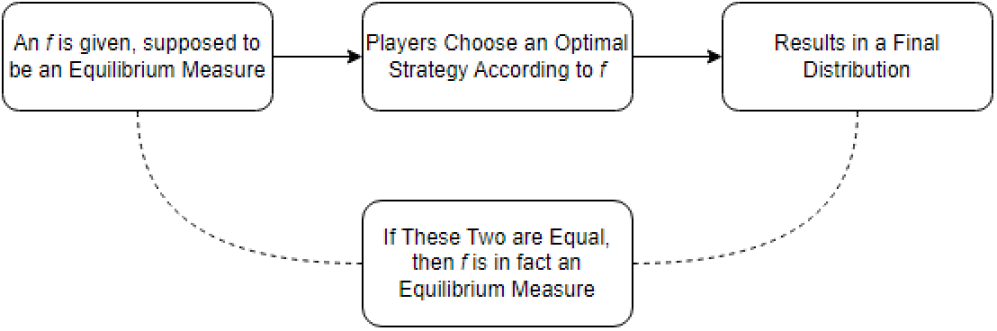
Figure 1. Mean Field Games Diagram

In this article, our purpose is two-fold:

1. prove there exists a unique Nash equilibrium, and

2. compute solutions using a numerical method.

As far as we know, this constitutes the first result on existence and uniqueness of solutions to first-order mean field game with singular measures. Our approach relies on the fact that we take an entirely discrete measure, which allows us to rewrite the problem in an equivalent finite-dimensional formulation. Intuitively, all we need to compute is how each Dirac mass $a_{j}\delta_{x_{j}}$ in the initial distribution will “fan out” into a density of total mass $a_{j}$ centered around point $x_{j}$. As explained below, the precise shape of this density is known through a priori considerations. This approach makes the problem amenable to classical methods. We believe it also provides geometric insight for what is going on more generally in density-penalized mean field games of first order.

Remark 1.1.

The main results of this article were first announced in the second author’s undergraduate thesis [Zim24].

2. Reformulation of the equilibrium problem

Let $\pi$ be an equilibrium, and let $f$ be the corresponding final density.

Definition 2.1.

The support of $\pi$, supp $\pi$, is the set of all $(x,y)$ such that, for all $\epsilon>0$, $\pi(B_{\epsilon}(x,y))>0,$ where $B_{\epsilon}(x,y)=\mathinner{\left\{(z,w)|\sqrt{(x-z)^{2}+(y-w)^{2}}<\epsilon\right\}}$, or, equivalently, $\pi(U)>0$ for every open set containing $(x,y)$.

The support of $f$, $\operatorname{supp}f$, is the closure of the set of all $y$ such that $f(y)>0$.

Lemma 2.2.

If $(x,y)\in\operatorname{supp}\pi$, then $x=x_{j}$ for some $j$ and $y\in\operatorname{supp}f$. Conversely, if $y\in\operatorname{supp}f$, then there exists $x_{j}$ such that $(x_{j},y)\in\operatorname{supp}\pi$.

Proof.

If $(x,y)\in\operatorname{supp}\pi$, then for all $\epsilon>0$ we have $m(B_{\epsilon}(x))=\pi(B_{\epsilon}(x)\times{\mathbb{R}})>0$ and $\int_{B_{\epsilon}(y)}f(z)\operatorname{d\!}z=\pi({\mathbb{R}}\times B_{\epsilon}(y))>0$. It follows that $x=x_{j}$ for some $j$, and $y\in\operatorname{supp}f$ since for every $\epsilon>0$ there exists $z\in B_{\epsilon}(y)$ such that $f(z)>0$.

Conversely, suppose $y\in\operatorname{supp}f$. For every $\epsilon>0$, $\pi({\mathbb{R}}\times B_{\epsilon}(y))=\int_{B_{\epsilon}(y)}f>0$. Since $\pi({\mathbb{R}}\times B_{\epsilon}(y))=\sum_{j=1}^{n}\pi(\{x_{j}\}\times B_{\epsilon}(y))$, for each $\epsilon$ there is a $j$ such that $\pi(\{x_{j}\}\times B_{\epsilon}(y))>0$. We can then find a sequence $\epsilon_{k}\downarrow 0$ and a fixed $j$ such that $\pi(\{x_{j}\}\times B_{\epsilon_{k}}(y))>0$ for all $k$, which implies $(x_{j},y)\in\operatorname{supp}\pi$. ∎

Now if $(x_{j},y)\in\operatorname{supp}\pi$, the definition of equilibrium implies $y\in E_{j}$ where

$$E_{j}=\operatorname{argmin}\mathinner{\left\{y\mathrel{\mathop{\ordinarycolon}}\displaystyle{(x_{j}-y)^{2}}+f(y)\right\}},$$

i.e. $E_{j}$ is the set of minimizers $y$ for the cost $J(x_{j},y,f)$. By Lemma 2.2, $\operatorname{supp}f\subset\bigcup_{j=1}^{N}E_{j}$; the intuitive meaning is that every player must move into one of the sets $E_{j}$. On the other hand, for $y\in E_{j}$ we have $f(y)=C_{j}-{(x_{j}-y)^{2}}$, where

$$C_{j}=\min\mathinner{\left\{y\mathrel{\mathop{\ordinarycolon}}\displaystyle{(x_{j}-y)^{2}}+f(y)\right\}}.$$

Thus, $f$ is completely determined by $C_{j}$ and $E_{j}$, and these in turn are coupled by the definition of $E_{j}$. So how do we determine $C_{j}$ and $E_{j}$? A first clue is the following proposition, whose proof is elementary:

Proposition 2.3.

$E_{j}=\mathinner{\left\{y\mathrel{\mathop{\ordinarycolon}}C_{j}-{(x_{j}-y)^{2}}\geq\mathinner{\left(C_{k}-{(x_{k}-y)^{2}}\right)}_{+}\ \forall k\right\}}$, where $x_{+}\mathrel{\mathop{\ordinarycolon}}=\max\{x,0\}$.

Proof.

If $y\in E_{j}$, then ${(x_{j}-y)^{2}}+f(y)=C_{j}$, and at the same time ${(x_{k}-y)^{2}}+f(y)\geq C_{k}$ for all $k$ by definition of $C_{k}$. Recalling that $f\geq 0$, we see that $C_{j}-{(x_{j}-y)^{2}}=f(y)\geq\mathinner{\left(C_{k}-{(x_{k}-y)^{2}}\right)}_{+}$ for all $k$.

Conversely, suppose $y\notin E_{j}$. If $y\in E_{k}$ for some other $k$, then $C_{j}-{(x_{j}-y)^{2}}<f(y)=C_{k}-{(x_{k}-y)^{2}}$. If $y\notin\bigcup_{1}^{N}E_{k}$, then $f(y)=0$, hence $C_{j}-{(x_{j}-y)^{2}}<0$. It follows that $C_{j}-{(x_{j}-y)^{2}}<\mathinner{\left({C_{k}}-(x_{k}-y)^{2}\right)}_{+}$ for at least one $k$. ∎

Corollary 2.4.

Let $f_{j}(y)=C_{j}-{(x_{j}-y)^{2}}$. Then $f(y)=\max\mathinner{\left\{0,f_{1}(y),\ldots,f_{N}(y)\right\}}$ and $E_{j}=\mathinner{\left\{y\mathrel{\mathop{\ordinarycolon}}f(y)=f_{j}(y)\right\}}$.

Intuitively, all the players initially concentrated at $x_{j}$ should spread out according to the density function $f_{j}$ over the set $E_{j}$. We now make this intuition rigorous.

Proposition 2.5.

$E_{j}=\mathinner{\left\{y\mathrel{\mathop{\ordinarycolon}}(x_{j},y)\in\operatorname{supp}\pi\right\}}$, $\int_{E_{j}\setminus\hat{E}_{j}}f=0$, and $\int_{E_{j}}f=a_{j}$.

Proof.

If $(x_{j},y)\in\operatorname{supp}\pi$, then by definition of equilibrium, it follows that $y\in E_{j}$. Conversely, suppose $y\in E_{j}$. As explained below in Lemma 3.1, $E_{j}$ is an interval, and if $y$ is in the interior of that interval, then $y\notin\cup_{k\neq j}E_{k}$. By Corollary 2.4 and Lemma 2.2 we deduce that $(x_{j},y)\in\operatorname{supp}\pi$. If $y$ is on the boundary of $E_{j}$, there is a sequence $y_{k}\to y$ with $y_{k}$ in the interior of $E_{j}$, so $(x_{j},y_{k})\in\operatorname{supp}\pi$ and thus $(x_{j},y)\in\operatorname{supp}\pi$.

To prove the remaining statements, start with the following inequality:

(2.1) $$a_{j}=m(\{x_{j}\})=\pi\mathinner{\left(\{x_{j}\}\times{\mathbb{R}}\right)}=\pi\mathinner{\left(\{x_{j}\}\times E_{j}\right)}\leq\pi\mathinner{\left({\mathbb{R}}\times\hat{E}_{j}\right)}=\int_{E_{j}}f.$$

Summing over $j$, we get

(2.2) $$1=\sum_{j=1}^{n}a_{j}\leq\sum_{j=1}^{N}\int_{E_{j}}f=\int f=1.$$

It follows that $\int_{E_{j}}f=a_{j}$, as desired. ∎

With these results, we can now reformulate the problem using only the parameters $C_{1},\ldots,C_{n}$.

Definition 2.6.

For a given vector $C=(C_{1},\ldots,C_{n})\in{\mathbb{R}}^{n}$,

• let $f_{j}^{(C)}(x)=C_{j}-(x-x_{j})^{2}$ for $j=1,\ldots,n$;

• let $f^{(C)}(x)=\max\{f_{1}^{(C)}(x),\ldots,f_{n}^{(C)}(x),0\}$;

• let $E_{j}^{(C)}=\mathinner{\left\{x\mathrel{\mathop{\ordinarycolon}}f_{j}^{(C)}(x)=f^{(C)}(x)\right\}}$ for $j=1,\ldots,n$;

• let $F_{j}(C)=\int_{E_{j}}f(x)\operatorname{d\!}{x}$ for $j=1,\ldots,n$; and

• let $F(C)=\mathinner{\left(F_{1}(C),\ldots,F_{n}(C)\right)}$.

To better understand these definitions, consider the following image:

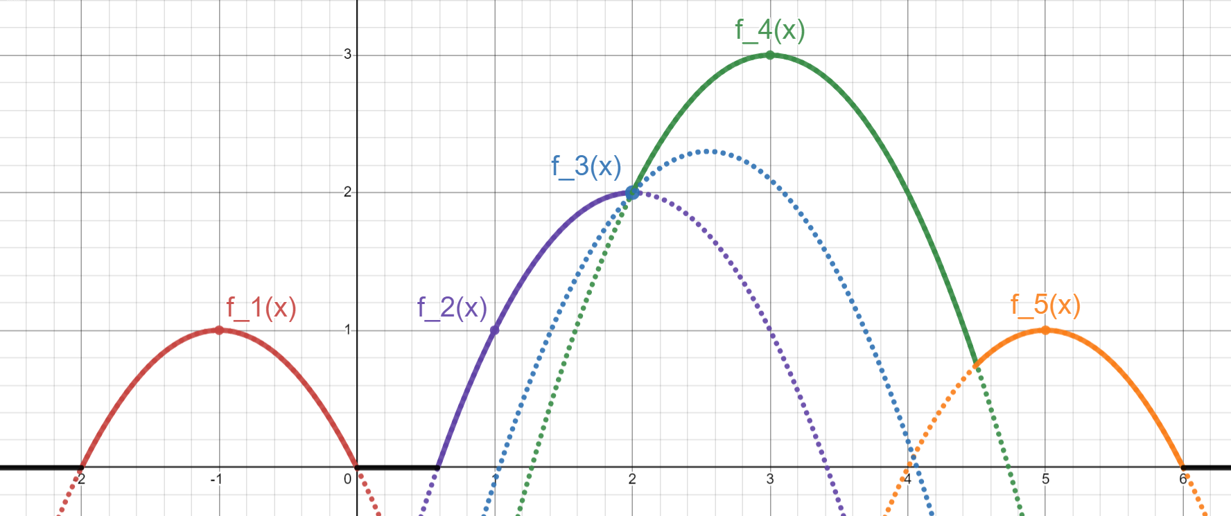
Figure 2. Visualization of the density $f(x)$

The graph of $f(x)$ is the solid-color part (i.e. the maximum). Each individual curve $f_{j}(x)$ can be thought of the density after the population sitting at point $x_{j}$ “fans out” and forms a “bubble” surrounding that point.

With these definitions, we now state the problem we wish to solve as follows:

Problem 2.7.

Given a vector $a=(a_{1},\ldots,a_{n})$, whose components are the weights in the discrete measure $m=\sum_{j=1}a_{j}\delta_{x_{j}}$, we want to find a vector $C$ such that $F(C)=a$.

By the arguments we have just given, if $f(x)$ is an equilibrium density, then $f(x)=f^{(C)}(x)$ where $C$ is the solution to Problem 2.7. Conversely, suppose $C$ is the solution to Problem 2.7 and let $f(x)=f^{(C)}(x)$. To see that $f(x)$ is an equilibrium density, first define a function $T\mathrel{\mathop{\ordinarycolon}}{\mathbb{R}}\to{\mathbb{R}}$ that sends every point in the interior of $E_{j}=E_{j}^{(C)}$ to the point $x_{j}$. Notice that $m$ is now the push-forward of the density through $T$. (We say a measure $\nu$ is the push-forward of a measure $\mu$ through a function $T$ if $\nu(B)=T\sharp\mu(B)\mathrel{\mathop{\ordinarycolon}}=\mu\mathinner{\left(T^{-1}(B)\right)}$; in this case $\nu=m$ and $\operatorname{d\!}\mu=f(x)\operatorname{d\!}x$.) Set $\pi$ to be the push-forward of the density $f$ by the function $y\mapsto(T(y),y)$. It follows that $\pi$ is an equilibrium.

We now state our main result:

Theorem 2.8 (Existence and uniqueness).

For each $a$ such that $a_{j}>0$ for $j=1,\dots,n$, there exists a unique $C$ such that $F(C)=a$.

Theorem 2.8 immediately implies the existence and uniqueness of a Nash equilibrium for any game where the initial distribution is discrete. We will prove Theorem 2.8 in two sections: Section 4 shows existence, and Section 5 proves uniqueness. These proofs rely on our analysis of $F(C)$ in Section 3, in which we establish certain formulas for $F_{j}(C)$ and its derivatives, prove continuity and coercivity, and the convexity of the effective domain of $F$ (namely, the set of all $C$ for which $F_{j}(C)>0$ for all $j$).

3. Structure of $F(C)$

The proof of Theorem 2.8 is based on various properties of $F(C)$, as given in Definition 2.6. Whenever $C$ is fixed, we will usually suppress the argument $C$ and simply write $f_{j}(x)$, $f(x)$, and $E_{j}$ instead of $f_{j}^{(C)}(x)$, $f^{(C)}(x)$, and $E_{j}^{(C)}$. In Section 3.1, we study the set $E_{j}$, namely the set over which $f(x)=f_{j}(x)$. We also study the effective domain of $F(C)$, over which we look for solutions to Problem 2.7, and we prove it is convex. In Section 3.2 we seek more or less explicit formulas for $F_{j}(C)$ and its derivatives. Section 3.3 shows that $F$ is a coercive function on certain domains, while Section 3.4 shows that it is continuous everywhere.

3.1. Properties of $E_{j}$

The most crucial points of interest will be the intersections between parabolas, namely where $f_{i}(x)=f_{j}(x)$, or $C_{i}-(x-x_{i})^{2}=C_{j}-(x-x_{j})^{2}$. We define the unique solution by

(3.1) $$\gamma_{ij}=\displaystyle\frac{C_{i}-C_{j}}{2(x_{j}-x_{i})}+\frac{x_{j}+x_{i}}{2},i\neq j.$$

Observe that if $f_{i}(x)>f_{j}(x)$ for all for $x<\gamma_{ij}$, then $f_{i}(x)<f_{j}(x)$ for all $x>\gamma_{ij}$, and likewise if $f_{i}(x)<f_{j}(x)$ for all for $x<\gamma_{ij}$, then $f_{i}(x)>f_{j}(x)$ for all $x>\gamma_{ij}$. With this in mind, we proceed to the following claim:

Lemma 3.1.

$E_{j}$ is either empty, a singleton, or a closed, bounded interval.

Proof.

We first note that, since $E_{j}$ is by definition is a set, $E_{j}$ is empty, a singleton, or contains at least two points. Hence, all we need to prove is that if $E_{j}$ contains more than one point, then $E_{j}$ is a closed, bounded interval. So, suppose that $E_{j}$ contains at least two points. Call two of these points $\alpha,\beta\in E_{j}$. Let $x\in(\alpha,\beta)$. To show that $E_{j}$ is an interval, we need to show that $x\in E_{j}$, i.e. $f_{j}(x)\geq f_{k}(x)$ and 0 for all $k\neq j$. Since $f$ is a concave function and both $f_{j}(\alpha)$ and $f_{j}(\beta)$ are greater than or equal to 0, $f_{j}(x)\geq 0$. To prove $f_{j}(x)\geq f_{k}(x)$ for all $k\neq j$, it suffices to show that there is no $\gamma_{jk}\in(\alpha,\beta)$. This can be shown simply using proof by contradiction: Suppose that there exists a $\gamma_{jk}\in(\alpha,\beta)$. Then, because of Remark 2.4, either $f_{j}(\alpha)>f_{k}(\alpha)$ and $f_{j}(\beta)<f_{k}(\beta)$, or $f_{j}(\alpha)<f_{k}(\alpha)$ and $f_{j}(\beta)>f_{k}(\beta)$. However, since both $\alpha_{j},\beta_{j}\in E_{j}$, neither of these possibilities can hold. Thus, $E_{j}$ must contain all the points between $\alpha$ and $\beta$. Next, to show that $E_{j}$ is bounded, we simply note that $E_{j}\subseteq{[\gamma_{ij},\gamma_{jk}]}$ for any $i<j<k$, and therefore is bounded. Lastly, to show $E_{j}$ is closed, we define $\mathinner{\left\{x_{k}\right\}}$ to be a sequence in $E_{j}$ such that $x_{k}\rightarrow x$. Thus, be definition of $E_{j}$, $f_{j}(x_{k})=f(x_{k})$. Since both $f_{j}(x)$ and $f(x)$ are continuous, letting $k\rightarrow\infty,f_{j}(x)=f(x)$. Therefore, if $E_{j}$ contains at least two points, then $E_{j}$ is a closed, bounded interval. ∎

In light of this, we introduce the following notation:

Definition 3.2.

In the case that $E_{j}$ is and interval, we define $\alpha_{j}$ and $\beta_{j}$ as the left and right end points of $E_{j}$, i.e. $[\alpha_{j},\beta_{j}]=E_{j}$. We denote the length of $E_{j}$ by $\mathinner{\!\left\lVert E_{j}\right\rVert}=\beta_{j}-\alpha_{j}$.

Before proceeding, we observe that Definition 2.6 leaves open the possibility that $F_{j}(C)=0$. Since we are trying to solve $F(C)=a$ where all the components of $a$ are positive, the true domain of interest is given as follows:

Definition 3.3.

$\mathbb{G}=\mathinner{\left\{C_{j}\mathrel{\mathop{\ordinarycolon}}F(C_{j})>0\text{ for }j=1,\dots,n\right\}}$.

Corollary 3.4.

If $C\in\mathbb{G}$, then $E_{j}$ is an interval for all $j=1,\dots,n.$

Proof.

First, by definition of $\mathbb{G}$, if $C\in\mathbb{G}$, then $F_{j}(C)>0$ for all $j=1,\dots,n$. Further, by Definition 2.6, it is clear that, in order for $F_{j}(C)$ to be greater than $0$, then $E_{j}$ cannot be empty or a singleton. Thus, by 3.1, if $F(C)\in\mathbb{G}$, then $E_{j}$ must be an interval for all $j=1,\dots,n$. ∎

Lemma 3.5.

For $C\in\mathbb{G}$, $\alpha_{j}$ and $\beta_{j}$ are continuous functions of $C$ given by

(3.2) $$\alpha_{j}=\begin{cases}\displaystyle\frac{C_{j-1}-C_{j}}{2(x_{j}-x_{j-1})}+\frac{x_{j}+x_{j-1}}{2}\text{ if }f_{j}(\alpha_{j})>0,\\ x_{j}-\sqrt{C_{j}},\text{ if }f_{j}(\alpha_{j})=0,\end{cases}\beta_{j}=\begin{cases}\displaystyle\frac{C_{j}-C_{j+1}}{2(x_{j+1}-x_{j})}+\frac{x_{j+1}+x_{j}}{2},\text{ if }f_{j}(\beta_{j})>0,\\ x_{j}+\sqrt{C_{j}},\text{ if }f_{j}(\beta_{j})=0.\end{cases}$$

Proof.

As $f=\max{(f_{1},f_{2},\dots,f_{n},0)}$, $\alpha_{j}$ is either $\gamma_{(j-1)j}$ if $f_{j}(\alpha_{j})>0$ or the leftmost root of $f_{j}(x)$. Likewise, $\beta_{j}$ is either $\gamma_{j(j+1)}$ or the rightmost root of $f_{j}(x)$. We already have an equation for $\gamma_{ij}$ in (3.1), so all that remains is to find when $f_{j}(x)=0$, which we do as follows:

$$f_{j}(x)=0\Rightarrow C_{j}-(x-x_{j})^{2}=0\Rightarrow x=x_{j}\pm\sqrt{C_{j}}.$$

The claim follows. ∎

Corollary 3.6.

If $C\in{\mathbb{G}}$, then the length of $E_{j}(C)$ is given by

(3.3) $$\mathinner{\!\left\lVert E_{j}\right\rVert}=k_{j}(C)=\min\{\gamma_{j,j+1}(C),x_{j}+\sqrt{C_{j}}\}-\max\{\gamma_{j-1,j}(C),x_{j}-\sqrt{C_{j}}\}.$$

In fact, $C\in{\mathbb{G}}$ if and only if $k_{j}(C)>0$ for all $j$. In particular, ${\mathbb{G}}$ is a convex set.

Proof.

If $C\in{\mathbb{G}}$, use Lemma 3.5 to see that $\mathinner{\!\left\lVert E_{j}\right\rVert}=\beta_{j}-\alpha_{j}=k_{j}(C)>0$. If $C\notin{\mathbb{G}}$, then at least one $E_{j}$ must be a singleton or empty, i.e. $f_{j}(x)$ is never the maximum in $f(x)=\max\{f_{1}(x),\ldots,f_{n}(x),0\}$. We deduce that one of the following inequalities must be false:

1. $\gamma_{j(j+1)}<\gamma_{(j-1)j}$

2. $\gamma_{(j-1)j}>x_{j}+\sqrt{C_{j}}$

3. $\gamma_{j(j+1)}<x_{j}-\sqrt{C_{j}}$

hence $k_{j}(C)\leq 0$.

Since $k_{j}(C)$ is a concave function and ${\mathbb{G}}=\{C\mathrel{\mathop{\ordinarycolon}}k_{j}(C)>0\ \forall j\}$, it follows that ${\mathbb{G}}$ is convex. ∎

We make one more simple observation about ${\mathbb{G}}$.

Lemma 3.7.

$\mathbb{G}$ is non-empty.

Proof.

To show $\mathbb{G}$ is non-empty, by 3.3, we need a $C$ such that $F_{j}(C)>0$ for all $j=1,\dots,n$. So, let $\epsilon>0$. Choose $\epsilon$ small enough so that, if $C_{j}=\epsilon$ for all $j=1,\dots,n$, then $f_{j}(\alpha_{j})=0=f_{j}(\beta_{j})$ for all $j=1,\dots,n$, i.e. no $f_{j}$ intersects any $f_{i},i\neq j$ above the $x$-axis. Then $E_{j}=[x_{j}-\sqrt{\epsilon},x_{j}+\sqrt{\epsilon}]$ for all $j=1,\dots,n$. Thus, we have

(3.4) $$F_{j}(C)=\frac{4}{3}\epsilon^{3/2},$$

which is greater than $0$. Thus, $\mathbb{G}$ is non-empty. ∎

Thus, the set $\mathbb{G}$ is both non-empty and convex, which will be useful in the proof of uniqueness of equilibria.

3.2. Computing $F_{j}(C)$ and its Derivatives

In this section, we want to calculate $F_{j}(C)$ and all of its derivatives for $C\in\mathbb{G}$. So, we have the following:

Proposition 3.8.

$F_{j}(C)=C_{j}(\beta_{j}-\alpha_{j})-\frac{1}{3}(\beta_{j}-x_{j})^{3}+\frac{1}{3}(\alpha_{j}-x_{j})^{3}$.

Proof.

We can compute this explicitly:

(3.5) $$F_{j}(C)=\int_{\alpha_{j}}^{\beta_{j}}C_{j}-(x-x_{j})^{2}\operatorname{d\!}x=C_{j}(\beta_{j}-\alpha_{j})-\frac{1}{3}(\beta_{j}-x_{j})^{3}+\frac{1}{3}(\alpha_{j}-x_{j})^{3}.$$

In particular, taking into account the different possibilities for $\alpha_{j}$ and $\beta_{j}$ (see 3.2):

$$\begin{split}&F_{j}(C)=\int_{\alpha_{j}}^{\beta_{j}}C_{j}-(x-x_{j})^{2}\operatorname{d\!}x=C_{j}(\beta_{j}-\alpha_{j})-\frac{1}{3}(\beta_{j}-x_{j})^{3}+\frac{1}{3}(\alpha_{j}-x_{j})^{3}\\ &\text{If }f_{j}(\alpha_{j}),f_{j}(\beta_{j})>0,\\ &F_{j}(C)=C_{j}\mathinner{\left(\frac{C_{j}-C_{j+1}}{2(x_{j+1}-x_{j})}+\frac{x_{j+1}+x_{j}}{2}\right)}-\frac{1}{3}\mathinner{\left(\frac{C_{j}-C_{j+1}}{2(x_{j+1}-x_{j})}+\frac{x_{j+1}+x_{j}}{2}-x_{j}\right)}^{3}\\ &-C_{j}\mathinner{\left(\frac{C_{j-1}-C_{j}}{2(x_{j}-x_{j-1})}+\frac{x_{j}+x_{j-1}}{2}\right)}+\frac{1}{3}\mathinner{\left(\frac{C_{j-1}-C_{j}}{2(x_{j}-x_{j-1})}+\frac{x_{j}+x_{j-1}}{2}-x_{j}\right)}^{3},\\ &\text{or if }f_{j}(\alpha_{j}),f_{j}(\beta_{j})=0,\\ &F_{j}(C)=\mathinner{\left(C_{j}(x_{j}+\sqrt{C_{j}})-\frac{1}{3}(x_{j}+\sqrt{C_{j}}-x_{j})^{3}\right)}-\mathinner{\left(C_{j}(x_{j}-\sqrt{C_{j}})-\frac{1}{3}(x_{j}-\sqrt{C_{j}}-x_{j})^{3}\right)}=\frac{4}{3}C_{j}^{3/2}.\end{split}$$

The other two cases, when $f_{j}(\alpha_{j})>0,f_{j}(\beta_{j})=0$ and when $f_{j}(\alpha_{j})=0,f_{j}(\beta_{j})>0$, are straightforward variations of these two cases. ∎

Remark 3.9.

These calculations show that, in particular, $0\leq F_{j}(C)\leq\frac{4}{3}C_{j}^{3/2}$ for any $C$. This will be useful later.

Proposition 3.10.

$\displaystyle\mathinner{\dfrac{\partial{}F_{j}(C)}{\partial{C_{j}}}}({C})=\mathinner{\!\left\lVert E_{j}\right\rVert}+\frac{f_{j}(\beta_{j})}{2(x_{j+1}-x_{j})}+\frac{f_{j}(\alpha_{j})}{2(x_{j}-x_{j-1})}$

Proof.

With $F(C)$ now calculated, we can easily calculate $\mathinner{\dfrac{\partial{}F_{j}(C)}{\partial{C_{j}}}}$, taking into account the different possibilities for $\alpha_{j}$ and $\beta_{j}$ as above:

(3.6) $$\begin{split}&\text{If }f_{j}(\alpha_{j}),f_{j}(\beta_{j})>0,\\ \mathinner{\dfrac{\partial{}F_{j}(C)}{\partial{C_{j}}}}=&\mathinner{\left(\frac{C_{j}-C_{j+1}}{2(x_{j+1}-x_{j})}+\frac{x_{{j+1}}+x_{j}}{2}\right)}+\mathinner{\left(\frac{C_{j}}{2(x_{j+1}-x_{j})}\right)}-{\frac{1}{2(x_{j+1}-x_{j})}}\mathinner{\left(\frac{C_{j}-C_{j+1}}{2(x_{j+1}-x_{j})}+\frac{x_{{j+1}}-x_{j}}{2}\right)}^{2}\\ -&\mathinner{\left(\frac{C_{j-1}-C_{j}}{2(x_{j}-x_{j-1})}+\frac{x_{j}+x_{j-1}}{2}\right)}+\mathinner{\left(\frac{C_{i}}{2(x_{j}-x_{j-1})}\right)}-{\frac{1}{2(x_{j}-x_{j-1})}}\mathinner{\left(\frac{C_{j-1}-C_{j}}{2(x_{j}-x_{j-1})}-\frac{x_{j}-x_{j-1}}{2}\right)}^{2}\\ =&\mathinner{\!\left\lVert E_{j}\right\rVert}+\frac{f_{j}(\beta_{j})}{2(x_{j+1}-x_{j})}+\frac{f_{j}(\alpha_{j})}{2(x_{j}-x_{j-1})},\\ &\text{or if }f_{j}(\alpha_{j}),f_{j}(\beta_{j})=0,\\ \mathinner{\dfrac{\partial{}F_{j}(C)}{\partial{C_{j}}}}=&\ 2C_{j}.\end{split}$$

Again, the other two cases are straightforward adaptations. In any case, we have:

(3.7) $$\mathinner{\dfrac{\partial{}F_{j}(C)}{\partial{C_{j}}}}=\mathinner{\!\left\lVert E_{j}\right\rVert}+\frac{f_{j}(\beta_{j})}{2(x_{j+1}-x_{j})}+\frac{f_{j}(\alpha_{j})}{2(x_{j}-x_{j-1})}.\\$$

Notice that this holds for every case, as if $f_{j}(\alpha_{j}),f_{j}(\beta_{j})=0$, then those components of the partial derivative would be 0, leaving $\mathinner{\!\left\lVert E_{j}\right\rVert}$, which is in fact $2C_{j}$ in that case. ∎

Theorem 3.11.

$\mathinner{\dfrac{\partial{}F_{i}(C)}{\partial{C_{j}}}}=\displaystyle\frac{-f_{i}(\gamma_{ij})}{2(x_{j}-x_{i})}$ and $\mathinner{\dfrac{\partial{}F_{j}(C)}{\partial{C_{i}}}}=\displaystyle\frac{-f_{j}(\gamma_{ij})}{2(x_{j}-x_{i})}$

Proof.

We now seek to calculate all $\mathinner{\dfrac{\partial{}F_{j}(C)}{\partial{C_{i}}}}$ for $i\neq j$. Without loss of generality, assume $i<j$. So, we only need to calculate $\displaystyle\mathinner{\dfrac{\partial{}F_{j}(C)}{\partial{C_{i}}}}$ and $\displaystyle\mathinner{\dfrac{\partial{}F_{i}(C)}{\partial{C_{j}}}}$. Further, if $f_{j}(x)$ does not touch $f_{i}(x)$ on or above the $x$-axis, then $\mathinner{\dfrac{\partial{}F_{j}(C)}{\partial{C_{i}}}}=0$, as slight changes in $C_{i}$ won’t change $C_{j}$. So we only consider the case if $f_{j}(\alpha_{j}),f_{j}(\beta_{j})>0$. We simply differentiate:

(3.8) $$\mathinner{\dfrac{\partial{}F_{i}(C)}{\partial{C_{j}}}}=\frac{1}{2(x_{j}-x_{i})}\mathinner{\left(\mathinner{\left(\frac{C_{i}-C_{j}}{2(x_{j}-x_{i})}+\frac{x_{j}-x_{i}}{2}\right)}^{2}-C_{i}\right)}=\frac{-f_{i}(\gamma_{ij})}{2(x_{j}-x_{i})}$$

(3.9) $$\mathinner{\dfrac{\partial{}F_{j}(C)}{\partial{C_{i}}}}={\frac{1}{2(x_{j}-x_{i})}\mathinner{\left(\mathinner{\left(\frac{C_{i}-C_{j}}{2(x_{j}-x_{i})}-\frac{x_{j}-x_{i}}{2}\right)}^{2}-C_{j}\right)}}=\frac{-f_{j}(\gamma_{ij})}{2(x_{j}-x_{i})}=\frac{-f_{i}(\gamma_{ij})}{2(x_{j}-x_{i})}$$

∎

We notice the following:

Remark 3.12.

$$\mathinner{\dfrac{\partial{}F_{i}(C)}{\partial{C_{j}}}}=\mathinner{\dfrac{\partial{}F_{j}(C)}{\partial{C_{i}}}}$$

Additionally, we observe that $\mathinner{\dfrac{\partial{}F_{i}(C)}{\partial{C_{j}}}}$ for any $i$ and $j$ depends on at most three components of $C$, as $\alpha_{j}$ and $\beta_{j}$ each only depend on one $C_{i}$ other than $C_{j}$ itself. With this in mind, we can say:

Lemma 3.13.

$\mathinner{\dfrac{\partial{}F_{i}(C)}{\partial{C_{j}}}}\neq 0$ for at most three components of $C$: $C_{j-1},C_{j},$ and $C_{j+1}$

3.3. Coercivity

We say that the vector field $F(C)$ is coercive provided that $\displaystyle\lim\limits_{\mathinner{\!\left\lVert C\right\rVert}\to\infty}\frac{F(C)\cdot C}{\mathinner{\!\left\lVert C\right\rVert}}=\infty$, where $\mathinner{\!\left\lVert C\right\rVert}=\mathinner{\left(C_{1}^{2}+\cdots+C_{n}^{2}\right)}^{1/2}$ is the norm of the vector $C$. This is the usual condition for a vector field to be surjective, as in the Minty-Browder Theorem [Bro67]. There is no chance for $F(C)$ to be coercive on all of ${\mathbb{R}}^{n}$, since $F_{j}(C)=0$ whenever $C_{j}\leq 0$. However, this will not matter, is we are always aiming at restricting to vectors $C$ with non-negative components. Instead, we will use the following substitute for coercivity to prove existence of solutions.

Lemma 3.14.

There exist constants $\delta\in(0,1)$ and $M>0$ such that if $C_{j}=\max\{C_{1},...,C_{n}\}\geq M$, then $F_{j}(C)\geq\delta C_{j}$.

Proof.

Choose a $C_{j}$ such that $C_{j}=\{C_{1},...,C_{n}\}$. We now seek to estimate $F_{j}({C})$. Note that $E_{j}$ must be an interval. The smallest $E_{j}$ could be is if $\beta_{j-1}=\alpha_{j}$ and $\beta_{j}=\alpha_{j+1}$. In this case, we can compute $\alpha_{j}$ and $\beta_{j}$:

$$\alpha_{j}=\frac{C_{j-1}-C_{j}}{2(x_{j}-x_{j-1})}+\frac{x_{j-1}+x_{j}}{2}\text{ , }\beta_{j}=\frac{C_{j}-C_{j+1}}{2(x_{j+1}-x_{j})}+\frac{x_{j}+x_{j+1}}{2},$$

and by the maximality of $C_{j}$ we get

$$\alpha_{j}\leq\frac{x_{j-1}+x_{j}}{2},\quad\beta_{j}\geq\frac{x_{j}+x_{j+1}}{2}.$$

This gives a lower bound on how close $\alpha_{j}$ and $\beta_{j}$ can get to $x_{j}$. Thus,

$$\begin{split}F_{j}({C})\geq\int_{\frac{x_{j-1}+x_{j}}{2}}^{\frac{x_{j}+x_{j+1}}{2}}C_{j}-(x-x_{j})^{2}\operatorname{d\!}x=C_{j}\frac{x_{j+1}-x_{j-1}}{2}-\frac{1}{3}\mathinner{\left(\mathinner{\left(\frac{x_{j+1}-x_{j}}{2}\right)}^{3}-\mathinner{\left(\frac{x_{j}-x_{j-1}}{2}\right)}^{3}\right)}.\end{split}$$

Define

$$\bar{\delta}\mathrel{\mathop{\ordinarycolon}}=\frac{\min_{j}\mathinner{\left\{x_{j+1}-x_{j-1}\right\}}}{2},\quad\bar{M}\mathrel{\mathop{\ordinarycolon}}=\frac{1}{3}\max_{j}\mathinner{\left(\mathinner{\left(\frac{x_{j+1}-x_{j}}{2}\right)}^{3}-\mathinner{\left(\frac{x_{j}-x_{j-1}}{2}\right)}^{3}\right)}_{+},$$

where we recall $x_{+}\mathrel{\mathop{\ordinarycolon}}=\max\{x,0\}$. Then

$$F_{j}(C)\geq\bar{\delta}C_{j}-\bar{M}.$$

Pick any $0<\delta<\min\{\bar{\delta},1\}$ and set $M=(\bar{\delta}-\delta)^{-1}\bar{M}$. If $C_{j}\geq M$, we get $F_{j}(C)\geq\delta C_{j}$, as desired. ∎

We remark that Lemma 3.14 can be used to prove that $F$ is coercive on ${\mathbb{R}}^{n}_{\geq 0}$, which is defined to be the set of all $(x_{1},\ldots,x_{n})$ such that $x_{j}\geq 0$ for every $j$. The reason is that if $C\in{\mathbb{R}}^{n}_{\geq 0}$ and $C_{j}=\max\{C_{1},\ldots,C_{n}\}$, then

$$F(C)\cdot C\geq F_{j}(C)C_{j}.$$

For the remaining details, let us first define the norm

$$\mathinner{\!\left\lVert x\right\rVert}_{\infty}=\max\mathinner{\left\{\mathinner{\!\left\lvert x_{1}\right\rvert},\ldots,\mathinner{\!\left\lvert x_{n}\right\rvert}\right\}}$$

and note that $\mathinner{\!\left\lVert x\right\rVert}_{\infty}=\max\{x_{1},\ldots,x_{n}\}$ for $x\in{\mathbb{R}}^{n}_{\geq 0}$. Recall that

$$\mathinner{\!\left\lVert x\right\rVert}_{\infty}\leq\mathinner{\!\left\lVert x\right\rVert}\leq\sqrt{n}\mathinner{\!\left\lVert x\right\rVert}_{\infty}.$$

Let $M,\delta$ be as in Lemma 3.14. If $C\in{\mathbb{R}}^{n}_{\geq 0}$ and $\mathinner{\!\left\lVert C\right\rVert}\geq M\sqrt{n}$, then $\mathinner{\!\left\lVert C\right\rVert}_{\infty}\geq M$ and so

$$F(C)\cdot C\geq F_{j}(C)C_{j}\geq\delta C_{j}^{2}=\delta\mathinner{\!\left\lVert C\right\rVert}_{\infty}^{2}\geq\frac{\delta}{\sqrt{n}}\mathinner{\!\left\lVert C\right\rVert}^{2}.$$

Thus $F$ is coercive on ${\mathbb{R}}^{n}_{\geq 0}$. However, we also note that only Lemma 3.14, and not coercivity per se, will be used directly to prove the existence of solutions.

3.4. Continuity

With coercivity proved, we move to prove that $F(C)$ is continuous. Before doing so, we need to explore what happens in $E_{j}=\varnothing$.

Lemma 3.15.

Let $I\subseteq{1,\dots,n}$ and $\mathcal{C}_{I}$ be the set of all $C$ such that $E_{j}(C)=\varnothing$ for all $j\in I$. Then $\mathcal{C}_{I}$ is open, i.e. for every $C\in\mathcal{C}_{I}$, there exists $\epsilon>0$ such that, if $\mathinner{\!\left\lVert\tilde{C}-C\right\rVert}<\epsilon$, then $\tilde{C}\in\mathcal{C}_{I}$.

Proof.

Let $C\in{\mathcal{C}}_{I}$. Define $\tilde{f}^{(C)}(x)=\max\{f_{j}^{(C)}(x)\mathrel{\mathop{\ordinarycolon}}j\in I\}$. Then $f^{(C)}(x)>\tilde{f}^{(C)}(x)$ for all $x$, because all of the sets $E_{j}(C)$, $j\in I$, are empty. Since all of the $f_{j}^{(C)}(x)$ are parabolas that go to $-\infty$ as $\mathinner{\!\left\lvert x\right\rvert}\to\infty$, there exists $M>0$ such that if $\mathinner{\!\left\lvert x\right\rvert}>M$, then $f^{(C)}(x)-\tilde{f}^{(C)}(x)\geq 1$. Now $f^{(C)}(x)-\tilde{f}^{(C)}(x)$ is a continuous and positive function, hence it has a minimum $\delta>0$ on the compact set $[-M,M]$. Without loss of generality, we can assume $\delta\leq 1$; in particular, we have $f^{(C)}(x)-\tilde{f}^{(C)}(x)\geq\delta$ for every $x$. Now assume $\mathinner{\!\left\lvert\tilde{C}_{j}-C_{j}\right\rvert}<\delta/2$ for $j=1,2,\ldots,n$. Then $\mathinner{\!\left\lvert f_{j}^{(\tilde{C})}(x)-f_{j}^{(C)}(x)\right\rvert}<\delta/2$ for every $j$ and every $x$. It follows that $\mathinner{\!\left\lvert f^{(\tilde{C})}(x)-f^{(C)}(x)\right\rvert}<\delta/2$ and $\mathinner{\!\left\lvert\tilde{f}^{(\tilde{C})}(x)-\tilde{f}^{(C)}(x)\right\rvert}<\delta/2$, so

(3.10) $$\begin{split}f^{(\tilde{C})}(x)-\tilde{f}^{(\tilde{C})}(x)&=f^{(\tilde{C})}(x)-f^{(C)}(x)+f^{(C)}(x)-\tilde{f}^{(C)}(x)+\tilde{f}^{(C)}(x)-\tilde{f}^{(\tilde{C})}(x)\\ &>-\delta/2+\delta-\delta/2=0.\end{split}$$

It follows that all the sets $E_{j}(\tilde{C})$, $j\in I$, are empty, and so $\tilde{C}$ must also be in ${\mathcal{C}}_{I}$. Thus, $\mathcal{C}_{I}$ is open. ∎

With this in mind, we can now prove continuity:

Theorem 3.16.

$F(C)$ is continuous.

Proof.

By Lemma 3.1, we know that $E_{j}$ is empty, a singleton, or is a closed, bounded interval. First, consider the case if $E_{j}=\varnothing$. Then $C\in\mathcal{C}_{I}$, as defined in Lemma 3.15. Take a sequence of vectors $C^{(k)}\rightarrow C$. Then, for $k$ sufficiently large, $C^{(k)}\in\mathcal{C}_{I}$ also. So $F_{j}(C^{(k)})=F_{j}(C)=0$ for every $j\in I$. Therefore, all the $j\in I$ will not effect the continuity of $F(C)$. In light of this, we can relabel the sequence $\mathinner{\left\{1,\dots,n\right\}}\setminus I$, calling it $\mathinner{\left\{1,\dots,m\right\}}$. Then $f(x)$ will still be the $\max\{f_{1}(x),f_{2}(x),\dots,f_{m}(x),0\}$, as those indices which may have been removed will not affect the max. Thus, we can assume for the remainder of this proof that $E_{j}(C)\neq\varnothing$, i.e. $j=1,\dots,m$.

Next, suppose that $E_{j}(C)$ is an interval. Choose a sequence of vectors $C^{(k)}\rightarrow C$. By equation (3.3), it is clear that, as $F_{j}(C)$ is simply a polynomial in terms of $C$, that $F_{j}(C^{(k)})\rightarrow F_{j}(C)$.

Lastly, suppose $E_{j}$ is a single point. Then, by the contra-positive of Corollary 3.4, $F_{j}(C)=0$. Again, we choose a sequence of vectors $C^{(k)}\rightarrow C$. So, we need to show $F_{j}(C^{(k)})\rightarrow 0$. If $F_{j}(C^{(k)})>0$ then $E_{j}(C^{(k)})$ is an interval whose length is given by $k_{j}(C^{(k)})$ defined in Corollary 3.6. Further, since $k_{j}(C)$ is a continuous function of $C$ and $E_{j}(C)$ is a single point, then $k_{j}(C^{(k)})\rightarrow 0$ as $k\rightarrow\infty$. Therefore, whenever $E_{j}(C^{(k)})$ is an interval, its length shrinks to zero as $k\rightarrow\infty$, and since in any other case we have $F_{j}(C^{(k)})=0$, we deduce that $F_{j}(C^{(k)})\rightarrow 0$ as $k\to\infty$. ∎

We have now sufficiently explored various properties of $f(x)$ and $F(C)$, so we may now move onto our first goal:

4. Proving Existence of a Solution

In this section, we seek to show that a solution $C$ to the equation $F(C)=a$ exists for all $a$. Before we begin the proof, we state Brouwer Fixed Point Theorem:

Lemma 4.1.

Every continuous function from a nonempty convex compact subset $K$ of a Euclidean space to $K$ itself has a fixed point.

See e.g. [Flo03]. We now begin the main result:

Theorem 4.2.

Let $a\in{\mathbb{R}}^{n}_{\geq 0}$, i.e. let $a=(a_{1},\ldots,a_{n})$ with $a_{j}\geq 0$ for each $j$. Then there exists a solution $C$ to the equation $F(C)=a$.

Proof.

Let $a$ be given. Define $L\mathrel{\mathop{\ordinarycolon}}\mathbb{R}^{n}_{\geq 0}\rightarrow\mathbb{R}^{n}_{\geq 0}$ as $L_{i}(C)\mathrel{\mathop{\ordinarycolon}}=\mathinner{\left(C_{i}+a_{i}-F_{i}(C)\right)}_{+}$ (recall $x_{+}\mathrel{\mathop{\ordinarycolon}}=\max\{x,0\}$). We will use the norm

$$\mathinner{\!\left\lVert C\right\rVert}_{1}\mathrel{\mathop{\ordinarycolon}}=\mathinner{\!\left\lvert C_{1}\right\rvert}+\cdots+\mathinner{\!\left\lvert C_{n}\right\rvert}=C_{1}+\cdots+C_{n}.$$

It is useful to recall that

$$\mathinner{\!\left\lVert C\right\rVert}_{\infty}\leq\mathinner{\!\left\lVert C\right\rVert}_{1}\leq n\mathinner{\!\left\lVert C\right\rVert}_{\infty}.$$

By Lemma 3.14, there exist constants $\delta\in(0,1)$ and $M>0$ such that if $C_{j}=\mathinner{\!\left\lVert C\right\rVert}_{\infty}\geq M$, then $F_{j}(C)\geq\delta C_{j}$. In this case,

$$L_{j}(C)\leq\mathinner{\left((1-\delta)C_{j}+a_{j}\right)}_{+}=(1-\delta)C_{j}+a_{j}.$$

In general,

$$L_{i}(C)\leq C_{i}+a_{i}.$$

Summing over all $i$, we deduce that

$$\mathinner{\!\left\lVert L(C)\right\rVert}_{1}\leq\mathinner{\!\left\lVert C\right\rVert}_{1}+\mathinner{\!\left\lVert a\right\rVert}_{1}-\delta C_{j}.$$

Recall that $C_{j}=\mathinner{\!\left\lVert C\right\rVert}_{\infty}\geq n^{-1}\mathinner{\!\left\lVert C\right\rVert}_{1}$. Let $r>\mathinner{\!\left\lVert a\right\rVert}_{1}n/\delta$. Then we have

(4.1) $$\mathinner{\!\left\lVert L(C)\right\rVert}_{1}\leq\mathinner{\!\left\lVert C\right\rVert}_{1}+\mathinner{\!\left\lVert a\right\rVert}_{1}-\delta n^{-1}\mathinner{\!\left\lVert C\right\rVert}_{1}<\mathinner{\!\left\lVert C\right\rVert}_{1}\quad\text{if}~{}\mathinner{\!\left\lVert C\right\rVert}_{1}\geq r.$$

We now restrict to a compact, convex set. Let $M_{r}$ be the set of all $x\in\mathbb{R}_{\geq 0}^{n}$ such that $\mathinner{\!\left\lVert x\right\rVert}_{1}\leq r$. Then $M_{r}$ is closed and bounded, so $M_{r}$ is compact, and it is clearly nonempty. Lastly, $M_{r}$ is convex, as it is the intersection of two convex sets, namely, ${\mathbb{R}}^{\geq 0}$ and the closed unit ball for the 1-norm. Thus, by Lemma 4.1, any continuous function $g\mathrel{\mathop{\ordinarycolon}}M_{r}\rightarrow M_{r}$ has a fixed point.

Define a function

(4.2) $$P(D)\mathrel{\mathop{\ordinarycolon}}=\begin{cases}\displaystyle D,\mathinner{\!\left\lVert D\right\rVert}_{1}\leq r\\ \frac{rD}{\mathinner{\!\left\lVert D\right\rVert}_{1}},\mathinner{\!\left\lVert D\right\rVert}_{1}>r.\end{cases}$$

Note that $P$ maps ${\mathbb{R}}^{n}_{\geq 0}$ into $M_{r}$. Finally, let $Q(C)\mathrel{\mathop{\ordinarycolon}}=P(L(C))$ for $C\in M_{r}$. Then $Q$ is continuous, as it is the composition of continuous functions, and it maps $M_{r}$ to itself. Thus, by 4.1, $Q$ has a fixed point $C\in M_{r}$. If $\mathinner{\!\left\lVert C\right\rVert}_{1}=r$, then

(4.3) $$r=\mathinner{\!\left\lVert C\right\rVert}_{1}=\mathinner{\!\left\lVert Q(C)\right\rVert}_{1}=\mathinner{\!\left\lVert P(L(C))\right\rVert}_{1}.$$

By construction of $P$, this implies

(4.4) $$\mathinner{\!\left\lVert L(C)\right\rVert}_{1}\geq r.$$

But this contradicts (4.1). It follows that $\mathinner{\!\left\lVert C\right\rVert}_{1}<r$. Thus,

(4.5) $$r>\mathinner{\!\left\lVert C\right\rVert}_{1}=\mathinner{\!\left\lVert Q(C)\right\rVert}_{1}=\mathinner{\!\left\lVert P(L(C))\right\rVert}_{1}.$$

Hence, $P(L(C))=L(C)$, so finally we have

(4.6) $$C=Q(C)=P(L(C))=L(C).$$

This implies that for each $i$,

$$C_{i}=\mathinner{\left(C_{i}+a_{i}-F_{i}(C)\right)}_{+}.$$

If $C_{i}>0$, this implies

$$C_{i}=C_{i}+a_{i}-F_{i}(C)\Rightarrow F_{i}(C)=a_{i}.$$

If $C_{i}=0$, then $F_{i}(C)=0$ and we get

$$0=\mathinner{\left(a_{i}\right)}_{+}=a_{i}$$

so again $F_{i}(C)=a_{i}$. Hence $F(C)=a$, as desired. ∎

5. Proving Uniqueness of a Solution

By Theorem 4.2, we know that a solution to $F(C)=a$ exists whenever $a\in{\mathbb{R}}^{n}_{\geq 0}$. It can be observed that, if one of the $a_{j}=0$, then the solution need not be unique; this occurs, for example, if one of the parabolas $f_{j}(x)$ lies entirely underneath another parabola $f_{k}(x)$, in which case adjusting $C_{j}$ slightly will not change the equality $F_{j}(C)=0$. Notice, however, that in such a case, one can simply throw out $a_{j}$ and reduce the dimension of the problem. Thus, without any loss of generality, we can assume $a_{j}>0$ for all $j$. We therefore have a solution $C\in\mathbb{G}$, where ${\mathbb{G}}$ is defined in Section 3.1.

In this section, we prove that the solution is unique. To do so, we show that $F(C)$ is strictly monotone in a classical sense. It is interesting to note that monotonicity is often used to prove uniqueness in mean field games, the most commonly used notion being the “Lasry-Lions monotonicity condition” (cf. [LL07]). (For a discussion on alternative monotonicity conditions, see [GM23].) Here, the coupling is indeed precisely through the density of players, and therefore the Lasry-Lions monotonicity condition holds. However, it is interesting to note that the monotonicity of $F(C)$, a function of the parameters $C_{1},\ldots,C_{n}$, is not a direct consequence the Lasry-Lions monotonicity condition in any obvious way.

Lemma 5.1.

On $\mathbb{G}$, $F(C)$ is strictly monotone, i.e. for any $C,\tilde{C}\in\mathbb{G},(F(C)-F(\tilde{C})(C-\tilde{C})>0$.

Proof.

Recall that $\mathbb{G}$ is convex by Corollary 3.6. To show F is strictly monotone, then, it suffices to show that

$$\sum_{i=1}^{n}\sum_{j=1}^{n}\mathinner{\dfrac{\partial{}F_{i}(C)}{\partial{C_{j}}}}\cdot(v_{i}v_{j})>0\ \forall\ {C},{v}\in\mathbb{R}^{n}\text{ with }v\neq 0.$$

Assume for the sake of notation that $v_{0}=0=v_{n+1}$. By Lemma 2.11,

$$S\mathrel{\mathop{\ordinarycolon}}=\sum_{i=1}^{n}\sum_{j=1}^{n}\mathinner{\dfrac{\partial{}F_{i}(C)}{\partial{C_{j}}}}v_{i}v_{j}=\displaystyle\sum_{j=1}^{n}\mathinner{\left(\mathinner{\dfrac{\partial{}F_{j}(C)}{\partial{C_{j}}}}(v_{j})^{2}+\mathinner{\dfrac{\partial{}F_{j}(C)}{\partial{C_{j-1}}}}(v_{{j-1}}v_{j})+\mathinner{\dfrac{\partial{}F_{j}(C)}{\partial{C_{j+1}}}}(v_{j}v_{{j+1}})\right)}.$$

Using the derivative formulas from (3.8),

$$S=\sum_{j=1}^{n}\mathinner{\left(\mathinner{\!\left\lVert E_{j}\right\rVert}+\frac{f_{j}(\alpha_{j})}{2(x_{j}-x_{j-1})}+\frac{f_{j}(\beta_{j})}{2(x_{j+1}-x_{j})}\right)}\mathinner{\left(v_{j}\right)}^{2}\\ -\mathinner{\left(\frac{f_{j}(\alpha_{j})}{2(x_{j}-x_{j-1})}\right)}\mathinner{\left(v_{j-1}v_{j}\right)}-\mathinner{\left(\frac{f_{j}(\beta_{j})}{2(x_{j+1}-x_{j})}\right)}\mathinner{\left(v_{j}v_{j+1}\right)}.$$

Since $f_{1}(\alpha_{1})=0=f_{n}(\beta_{n})$, we can rewrite this as

$$S=\sum_{j=1}^{n}{\mathinner{\!\left\lVert E_{j}\right\rVert}}{v_{j}}^{2}+\sum_{j=2}^{n}\mathinner{\left(\frac{f_{j}(\alpha_{j})}{2(x_{j}-x_{j-1})}\mathinner{\left(v_{j}\right)}^{2}-\mathinner{\left(\frac{f_{j}(\alpha_{j})}{2(x_{j}-x_{j-1})}\right)}\mathinner{\left(v_{j-1}v_{j}\right)}\right)}\\ +\sum_{j=1}^{n-1}\mathinner{\left(\frac{f_{j}(\beta_{j})}{2(x_{j+1}-x_{j})}\mathinner{\left(v_{j}\right)}^{2}-\mathinner{\left(\frac{f_{j}(\beta_{j})}{{2(x_{(j+1)}-x_{j})}}\right)}\mathinner{\left(v_{j}v_{j+1}\right)}\right)}.$$

Since $f_{j+1}(\alpha_{j+1})$ is either $f_{j}(\beta_{j})$ or $0$, we can combine to get

$$\begin{split}S=\displaystyle&\sum_{j=1}^{n}{\mathinner{\!\left\lVert E_{j}\right\rVert}}{v_{j}}^{2}+\sum_{j=1}^{n-1}\frac{f_{j}(\beta_{j})}{2(x_{j+1}-x_{j})}\mathinner{\left(v_{j+1}\right)}^{2}-\frac{2f_{j}(\beta_{j})}{2(x_{j+1}-x_{j})}\mathinner{\left(v_{j}v_{j+1}\right)}+\frac{f_{j}(\beta_{j})}{2(x_{j+1}-x_{j})}\mathinner{\left(v_{j}\right)}^{2}\\ =\displaystyle&\sum_{j=1}^{n}{\mathinner{\!\left\lVert E_{j}\right\rVert}}{v_{j}}^{2}+\sum_{j=1}^{n-1}\mathinner{\left(\frac{f_{j}(\beta_{j})}{2(x_{j+1}-x_{j})}\right)}\mathinner{\left(v_{j+1}-v_{j}\right)}^{2}>0.\end{split}$$

Thus, $F(C)$ is strictly monotone on $\mathbb{G}$. ∎

We now have everything we need to prove uniqueness.

Theorem 5.2.

The solution to the equation $F(C)=a$ has a unique solution.

Proof.

Suppose, for the sake of contradiction, that $C_{1},C_{2}\in\mathbb{G}$ with $C_{1}\neq C_{2}$ are both solutions to $F(C)=a$. Then $F(C_{1})=F(C_{2})$, so $(F(C_{1})-F(C_{2})(C_{1}-C_{2})=0$. But this contradicts 5.1. Thus, the solution to $F(C)$ is unique. ∎

We have now shown that a unique solution to $F(C)=a$ exists and is unique. We now move on to numerical approximations.

6. Numerical Simulations

We used Newton’s Method to find approximate solutions to $F(C)=a$. By algebraically solving $\frac{4}{3}C_{j}^{3/2}=a_{j}$, we obtain an initial guess $C=C^{(0)}$ such that $F_{j}(C)\leq a_{j}$ for each $j$ (see Remark 3.9). Then we define an approximating sequence $C^{(n)}$ by

(6.1) $$C^{(n+1)}=C^{(n)}-DF\mathinner{\left(C^{(n)}\right)}^{-1}\mathinner{\left(F\mathinner{\left(C^{(n)}\right)}-a\right)},$$

where $DF(C)$ is the Jacobian matrix computed in Section 3.2. The residual $\mathinner{\!\left\lVert F\mathinner{\left(C^{(n)}\right)}-a\right\rVert}$ can be computed easily; in practice it becomes vanishingly small after only a few iterations. Below we report on three simulations. In each case, the initial distribution $m=\sum_{j=1}^{n}a_{j}\delta_{x_{j}}$ is illustrated a set of $n$ bars located at position $x_{j}$ with height $a_{j}$. Then the final density $f(x)$ is then graphed over these bars. The function $f(x)$ is piecewise quadratic with the $j$th parabola centered at $x_{j}$ and representing the spreading of the population that starts at $x_{j}$; the area under this parabola above the $x$-axis equals $a_{j}$. This accords with our geometric intuition about the game: players spread out as much as possible so as to avoid areas of high population density, and the shape of the final density matches the quadratic cost $(x-y)^{2}$ of traveling from $x$ to $y$.

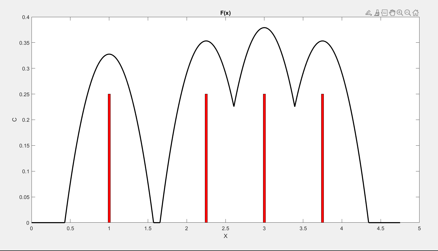
Figure 3. Example 1: $x=(1,2.25,3,3.75),a=(0.25,0.25,0.25,0.25)$

In the first simulation (Figure 3), we took an initial population uniformly distributed over four points: $m=\frac{1}{4}\mathinner{\left(\delta_{1}+\delta_{2.25}+\delta_{3}+\delta_{3.75}\right)}$. In this example, the leftmost quarter of the population is far enough away from rest that it can spread out without colliding with the others, whereas the other three are close enough to each other that players have less room to move, resulting in a narrower probability density.

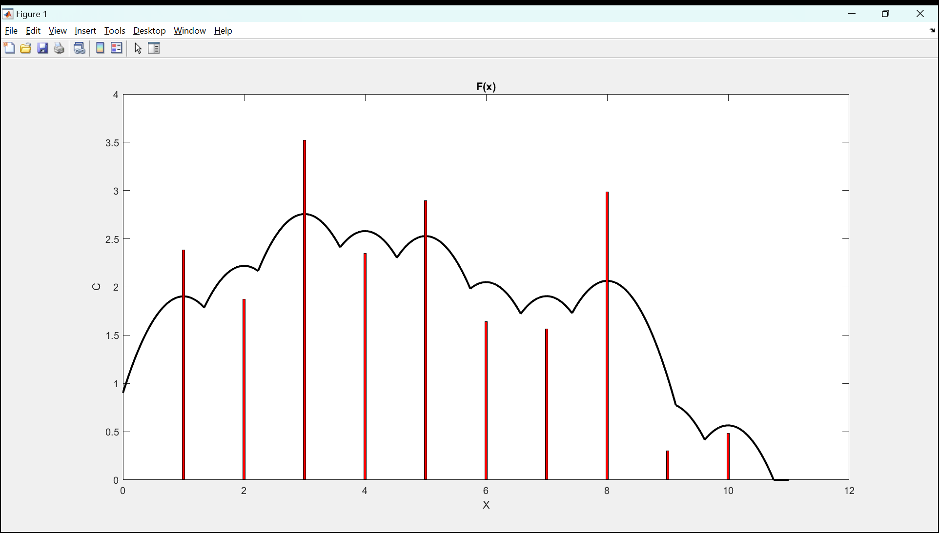
Figure 4. Example 2: $x=(1,2,\dots,10),a=random$

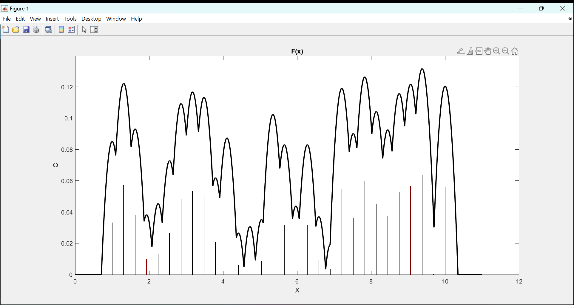
Figure 5. Example 3: $x=random$, $a=random$

In the second simulation (Figure 4), we let $x_{j}-x_{j-1}$ be constant and let $a$ be random. (Note that we did not normalize the components of $a$ to sum to 1, but this does not change the shape of the solution.) Notice how in this sample the probability density has a very interesting contour. For example, the “bubble” (i.e. piece of parabola) corresponding to $x=9$ barely appears because it is crowded by neighboring “bubbles.” This demonstrates how the different weights locally change the shape of the density.

In the last simulation (Figure 5), the vectors $x$ and $a$ are random (and $a$ is normalized to be a probability vector). Although the initial measure is highly irregular, the final density will still be smooth, though it appears less so as the number of random points are chosen. Indeed, as the proof of uniqueness in Section 5 suggests, the problem becomes more and more ill-conditioned as the points $x_{j}$ get closer together, since the lengths of the intervals $E_{j}$ necessarily get smaller.

7. Conclusion

In this paper we have studied a mean field game with final cost equal to the population density of players. We considered the case where the initial measure is discrete, which seems to be new in the literature. We showed that the problem reduces to a finite dimensional problem, which can prove is well-posed by classical methods. Our numerical simulations illustrate the “smoothing effect” that mean field games with density penalization are expected to have. For future research, it would be interesting to see if this approach could be extended to more general mean field games with density-dependent costs and discrete initial measures.

References

- [ACD+20] Yves Achdou, Pierre Cardaliaguet, François Delarue, Alessio Porretta, Filippo Santambrogio, Pierre Cardaliaguet, and Alessio Porretta. An introduction to mean field game theory. Mean Field Games: Cetraro, Italy 2019, pages 1–158, 2020.
- [BFY13] Alain Bensoussan, Jens Frehse, and Phillip Yam. Mean field games and mean field type control theory. Springer, 2013.
- [Bro67] F.E. Browder. Existence and perturbation theorems for nonlinear maximal monotone operators in Banach spaces. Bull. Amer. Math. Soc., 73:322–327, 1967.
- [Car15] Pierre Cardaliaguet. Weak solutions for first order mean field games with local coupling. In Analysis and Geometry in Control Theory and its Applications, volume 11 of Springer INdAM Series, pages 111–158. Springer, 2015.
- [CD17] R Carmona and F Delarue. Probabilistic Theory of Mean Field Games: vol. I, Mean Field FBSDEs, Control, and Games. Stochastic Analysis and Applications, Springer Verlag, 2017.
- [CG15] Pierre Cardaliaguet and P. Jameson Graber. Mean field games systems of first order. ESAIM: COCV, 21(3):690–722, 2015.
- [CGPT15] Pierre Cardaliaguet, P. Jameson Graber, Alessio Porretta, and Daniela Tonon. Second order mean field games with degenerate diffusion and local coupling. Nonlinear Differential Equations and Applications NoDEA, 22(5):1287–1317, 2015.
- [Flo03] Monique Florenzano. General equilibrium analysis: existence and optimality properties of equilibria. Springer Science & Business Media, 2003.
- [G+14] Diogo A Gomes et al. Mean field games models–a brief survey. Dynamic Games and Applications, 4(2):110–154, 2014.
- [GM18] P. Jameson Graber and Alpár R. Mészáros. Sobolev regularity for first order mean field games. Annales de l’Institut Henri Poincaré C, Analyse Non Linéaire, 35(6):1557–1576, September 2018.
- [GM23] P. Jameson Graber and Alpár R. Mészáros. On monotonicity conditions for mean field games. Journal of Functional Analysis, 285(9):110095, 2023.
- [Gra14] P Jameson Graber. Optimal control of first-order Hamilton–Jacobi equations with linearly bounded Hamiltonian. Applied Mathematics & Optimization, 70(2):185–224, 2014.
- [HMC06] Minyi Huang, Roland P Malhamé, and Peter E Caines. Large population stochastic dynamic games: closed-loop McKean-Vlasov systems and the nash certainty equivalence principle. Communications in Information & Systems, 6(3):221–252, 2006.
- [LL06a] Jean-Michel Lasry and Pierre-Louis Lions. Jeux à champ moyen. I–Le cas stationnaire. Comptes Rendus Mathématique, 343(9):619–625, 2006.
- [LL06b] Jean-Michel Lasry and Pierre-Louis Lions. Jeux à champ moyen. II–Horizon fini et contrôle optimal. Comptes Rendus Mathématique, 343(10):679–684, 2006.
- [LL07] Jean-Michel Lasry and Pierre-Louis Lions. Mean field games. Japanese Journal of Mathematics, 2(1):229–260, 2007.
- [Mun22] Sebastian Munoz. Classical and weak solutions to local first-order mean field games through elliptic regularity. Annales de l’Institut Henri Poincaré C, 39(1):1–39, 2022.
- [PS17] Adam Prosinski and Filippo Santambrogio. Global-in-time regularity via duality for congestion-penalized mean field games. Stochastics, 89(6-7):923–942, 2017.
- [Zim24] Brady Zimmerman. A finite dimensional approximation of a density dependent mean field game, 2024. Bachelor’s Thesis.