Sub-uniformity of harmonic mean p-values

Abstract

We obtain several inequalities on the generalized means of dependent p-values. In particular, the weighted harmonic mean of p-values is strictly sub-uniform under several dependence assumptions of p-values, including independence, weak negative association, the class of extremal mixture copulas, and some Clayton copulas. Sub-uniformity of the harmonic mean of p-values has an important implication in multiple hypothesis testing: It is statistically invalid to merge p-values using the harmonic mean unless a proper threshold or multiplier adjustment is used, and this invalidity applies across all significance levels. The required multiplier adjustment on the harmonic mean explodes as the number of p-values increases, and hence there does not exist a constant multiplier that works for any number of p-values, even under independence.

Keywords: Multiple hypothesis testing; merging function; p-value; stochastic order; negative dependence; Clayton copula.

1 Introduction

In multiple testing of a single hypothesis and testing multiple hypotheses, a decision maker often needs to combine several p-values into one p-value. Recently, Wilson (2019) proposed the harmonic mean p-value method, which belongs to the larger class of merging methods using generalized mean, studied by Vovk and Wang (2020). This class of generalized mean also includes Fisher’s combination method (Fisher (1948)) via the geometric mean, often applied under the assumption that p-values are independent. The harmonic mean p-value has some desirable properties such as being applicable under a wide range of dependence assumptions of p-values, and has received considerable attention from statistics and the natural sciences. Validity, admissibility, and threshold adjustments of the generalized mean methods for p-values with arbitrary dependence are studied further by Vovk et al. (2022) and Chen et al. (2023).

The harmonic mean p-value is known to be anti-conservative under some dependence structures, as noted by Wilson (2019). If the underlying dependence structure is arbitrary, a threshold correction of order $\log n$ is needed, where $n$ is the number of p-values to merge (Vovk and Wang (2020)). This correction generally leads to very conservative tests, and it may be reduced or even omitted under some specific dependence assumptions. In this paper, we study a stochastic order relation between a weighted generalized mean of standard uniform p-values and a standard uniform p-value under several dependence assumptions, and discuss its implications for the validity and threshold adjustment for harmonic mean p-values.

Let $\Delta_{n}=\{(w_{1},\dots,w_{n})\in[0,1]^{n}:w_{1}+\dots+w_{n}=1\}$ be the unit $n$-simplex. We always assume $n\geq 2$. For $r\in\mathbb{R}\setminus\{0\}$, $n\in\mathbb{N}$, and $\mathbf{w}=(w_{1},\dots,w_{n})\in\Delta_{n}$, the (weighted) $r$-mean function is defined as

$$M^{\mathbf{w}}_{r}(u_{1},\dots,u_{n})=\left(w_{1}u_{1}^{r}+\dots+w_{n}u_{n}^{r}\right)^{1/r},~{}~{}~{}~{}~{}(u_{1},\dots,u_{n})\in(0,\infty)^{n}.$$

The $0$-mean function is the weighted geometric mean, that is, $M^{\mathbf{w}}_{0}(u_{1},\dots,u_{n})=\prod_{i=1}^{n}u_{i}^{w_{i}},$ which is also the limit of $M^{\mathbf{w}}_{r}$ as $r\to 0$. If $w_{1}=\dots=w_{n}=1/n$, $M_{r}^{\mathbf{w}}$ is the symmetric $r$-mean function, denoted by $M_{r}$ for simplicity, and it is defined on $\bigcup_{n\in\mathbb{N}}(0,\infty)^{n}$. Denote by $\Delta^{+}_{n}=\Delta_{n}\cap(0,1)^{n}$. For some of our results, we will only consider $\mathbf{w}\in\Delta^{+}_{n}$ since if some components of $\mathbf{w}$ are zero, we can simply reduce the dimension of $M_{r}^{\mathbf{w}}$.

Throughout, $U_{1},\dots,U_{n}$ are (standard) uniform random variables on $(0,1)$ that are possibly dependent, and they represent p-values to combine. The quantity $M^{\mathbf{w}}_{r}(U_{1},\dots,U_{n})$ is the weighted $r$-mean of p-values. For two random variables $X$ and $Y$, we say $X$ is less than $Y$ in stochastic order, denoted by $X\preceq_{\rm st}Y$, if $\mathbb{P}(X\leq x)\geq\mathbb{P}(Y\leq x)$ for all $x\in\mathbb{R}$. Moreover, we write $X\simeq_{\rm st}Y$ if $X$ and $Y$ have the same distribution. The main results in this paper concern the following inequality under several dependence assumptions of $U_{1},\dots,U_{n}$

$$M^{\mathbf{w}}_{r}(U_{1},\dots,U_{n})\preceq_{\rm st}U_{1},$$ (1)

where $r\leq-1$. Relation (1) is quite strong as it requires $\mathbb{P}(M^{\mathbf{w}}_{r}(U_{1},\dots,U_{n})\leq p)\geq p$ to hold for all threshold levels $p\in(0,1)$. Note that (1) cannot hold for $r>-1$ except for identical $U_{1},\dots,U_{n}$ (see Proposition 1).

A non-negative random variable $X$ is said to be sub-uniform if $X\preceq_{\rm st}U_{1}$. Moreover, $X$ is strictly sub-uniform if

$$\mathbb{P}(X\leq p)>p~{}\mbox{ for all $p\in(0,1)$}.$$ (2)

Using a sub-uniform p-value is anti-conservative in hypothesis testing, since it has a larger type-I error rate than the nominal level. Therefore, if (1) holds true, then merging p-values using the harmonic mean, or any $r$-generalized mean function with $r\leq-1$, is anti-conservative across all significance levels in $(0,1)$.

Remark 1 (Terminology).

Although sub-uniformity is an important property for studying p-values, this term has been used with different meanings in the literature. Some of them are collected here. A non-negative random variable $X$ is called super-uniform by Barber and Ramdas, (2017) if $U_{1}\preceq_{\rm st}X$ (anticipating that sub-uniformity should be defined by flipping the above inequality, their terminology is consistent with ours), but such a random variable is called sub-uniform by Ferreira and Zwinderman, (2006). Moreover, Chen and Sarkar, (2020) defined sub-uniformity in the strict sense (2). Rubin-Delanchy et al., (2019) called $X$ sub-uniform if it is dominated by $U_{1}$ in convex order.

When mentioning (strict) sub-uniformity later in this paper, we always refer to the corresponding property of $M^{\mathbf{w}}_{r}(U_{1},\dots,U_{n})$ or $M_{r}(U_{1},\dots,U_{n})$ with $r\leq 1$, which will be clear from the context.

The main objective of this paper is to study (1) given several dependence assumptions of $U_{1},\dots,U_{n}$, including weak negative association (Proposition 4), the class of extremal mixture copulas (Theorem 1), and some Clayton copulas (Theorem 2). The notion of weak negative association includes multivariate normal distributions with non-positive correlations as special cases; see, e.g., Chi et al., (2022) for examples of negative dependence in multiple hypothesis testing. Some of our results are built on a recent study of Chen et al. (2024), where a stochastic ordering inequality on Pareto-type random variables is established. As discrete p-values may arise in hypothesis testing (e.g., Vovk et al. (2005)), we also study sub-uniformity for discrete uniform random variables on $\{1/m,\dots,m/m\}$ for $m\in\mathbb{N}$. This situation is quite different from the uniform case as (1) can never hold for $\mathbf{w}\in\Delta_{n}^{+}$ in the case of discrete uniform random variables unless they are identical. However, using the harmonic mean function to merge discrete uniform random variables can still be anti-conservative at some threshold levels (Theorem 3).

Most findings of this paper are negative results: Under many different assumptions of dependence among p-values, the harmonic mean p-value is anti-conservative and cannot be used without a proper adjustment, and the adjustment coefficient diverges even in the case of independence. To address these issues, while keeping the advantages of the harmonic mean p-value, it is recommendable to use the Simes method (Simes (1986)) or the Cauchy combination method (Liu and Xie (2020)), which are shown to be valid under various forms of dependence, and perform comparably to the harmonic mean p-value; see results in Chen et al. (2023) on comparing these three methods. Other methods based on heavy-tailed transformation of p-values can also be used under different assumptions (Gui et al. (2023)). An exception to the above negative results is the case of Clayton copulas treated in Theorem 2, where we obtain a positive result that the harmonic mean p-value can be made valid with a small threshold adjustment (a multiplicative factor of $1.131$) under the assumption of Clayton copulas with parameter at least $1$.

The rest of the paper is organized as follows. In Section 2, we first discuss the intuition behind (1) in the simplest case, and then present general properties related to sub-uniformity for dependent $U_{1},\dots,U_{n}$. In Section 3, (1) is shown given the aforementioned dependence assumptions of $U_{1},\dots,U_{n}$. In Section 4, the threshold of the harmonic mean p-value method is studied for independent p-values, where we see that the adjustment explodes at the rate of $\log n$ for a fixed probability level. Sub-uniformity for discrete uniform random variables is studied in Section 5. Numerical examples based on simple simulations are presented in Section 6, and Section 7 concludes the paper.

2 Some observations and general results on sub-uniformity

We set straight some first observations on the sub-uniformity inequality (1). First, the generalized mean is monotone in $r$; that is, given any $\mathbf{w}\in\Delta_{n}$, $M^{\mathbf{w}}_{r}\leq M^{\mathbf{w}}_{s}$ for $r\leq s$ (Theorem 16 in Hardy et al. (1934)). Hence, we have $M^{\mathbf{w}}_{r}(U_{1},\dots,U_{n})\leq M^{\mathbf{w}}_{-1}(U_{1},\dots,U_{n})$ for all $r\leq-1$. To get the sub-uniformity inequality (1) for all $r\leq-1$, it suffices to show

$$\mathbb{P}(M^{\mathbf{w}}_{-1}(U_{1},\dots,U_{n})\leq p)\geq p\mbox{~{}for all $p\in(0,1)$}.$$ (3)

This observation simplifies our journey by allowing us to focus on the case of harmonic mean, which also happens to be the most popular method within the class of generalized mean methods for $r\in(-\infty,0)$.

We begin with a simple proof for independent $U_{1},\dots,U_{n}$ in the symmetric case. Although (3) in this case directly follows from Theorem 1 of Chen et al. (2024), the proof below, different from Chen et al. (2024), helps to understand (3) via a result well-known in the multiple testing literature, namely the Simes inequality (Simes (1986)). For $(u_{1},\dots,u_{n})\in(0,\infty)^{n}$, the Simes function is defined as $S(u_{1},\dots,u_{n})=\min\{nu_{(i)}/i\}$ where $u_{(1)},\dots,u_{(n)}$ are the order statistics of $u_{1},\dots,u_{n}$, from the smallest to the largest. As shown by Simes (1986), $S(U_{1},\dots,U_{n})$ is uniformly distributed on $(0,1)$ given independent $U_{1},\dots,U_{n}$. Moreover, we have $M_{-1}\leq S$; this inequality is in Theorem 3 of Chen et al. (2023), but one can also check it directly. Putting these two observations together, we have

$$M_{-1}(U_{1},\dots,U_{n})\leq S(U_{1},\dots,U_{n})\simeq_{\rm st}U_{1},$$

which implies that (1) holds for symmetric mean of independent $U_{1},\dots,U_{n}$.

Before showing (1) holds under more general assumptions, we discuss several properties related to the target problem. We first explain that it is only meaningful to consider the sub-uniformity (1) for $r\leq-1$. Indeed, as illustrated in Proposition 1 below, sub-uniformity can hold for some $r>-1$ only in the trivial case that $U_{1},\dots,U_{n}$ are identical, and thus the strict uniformity can never hold for any $r>-1$. For $n\in\mathbb{N}$, write $[n]=\{1,\dots,n\}$.

Proposition 1.

The following statements are equivalent.

1. $M^{\mathbf{w}}_{r}(U_{1},\dots,U_{n})\preceq_{\rm st}U_{1}$ for some $r\in(-1,\infty)$ and $\mathbf{w}\in\Delta_{n}^{+}$;

2. $M^{\mathbf{w}}_{r}(U_{1},\dots,U_{n})\simeq_{\rm st}U_{1}$ for some $r\in(-1,\infty)$ and $\mathbf{w}\in\Delta_{n}^{+}$;

3. $U_{1}=\dots=U_{n}$ a.s.;

4. $M^{\mathbf{w}}_{r}(U_{1},\dots,U_{n})=U_{1}$ a.s. for all $r\in\mathbb{R}$ and all $\mathbf{w}\in\Delta_{n}$;

5. $M^{\mathbf{w}}_{r}(U_{1},\dots,U_{n})=U_{1}$ a.s. for some $r\in(-1,\infty)$ and $\mathbf{w}\in\Delta_{n}^{+}$.

Proof.

Note that the binary relation $X\preceq_{\rm st}Y$ is flipped under decreasing transformation on both $X$ and $Y$. Hence, for $r<0$, we can write $M^{\mathbf{w}}_{r}(U_{1},\dots,U_{n})\preceq_{\rm st}U_{1}$ as

$$\sum_{i=1}^{n}w_{i}U_{i}^{r}\succeq_{\rm st}U_{1}^{r}.$$ (4)

The case $r\geq 0$ can be argued similarly, and we will omit it from the discussion below.

(i)$\Rightarrow$(ii): If $\sum_{i=1}^{n}w_{i}U_{i}^{r}$ and $U_{1}^{r}$ are not identically distributed, then

$$\mathbb{E}\left[\sum_{i=1}^{n}w_{i}U_{i}^{r}\right]>\mathbb{E}\left[U_{1}^{r}\right],$$

which leads to a contradiction, since both expectations are equal to $1/(r+1)$. Hence, we have $\sum_{i=1}^{n}w_{i}U_{i}^{r}\simeq_{\rm st}U_{1}^{r}$.

(ii)$\Rightarrow$(iii): Let $U=M_{r}^{\mathbf{w}}(U_{1},\dots,U_{n})$, which is uniformly distributed on $[0,1]$. Note that

$$\sum_{i=1}^{n}w_{i}U_{i}^{r}=U^{r}.$$ (5)

Take $\epsilon\in(0,1+r)$. From (5), we have

$$\mathbb{E}\left[\sum_{i=1}^{n}w_{i}U_{i}^{r}U^{-\epsilon}\right]=\mathbb{E}\left[U^{r-\epsilon}\right]=\frac{1}{1+r-\epsilon}.$$ (6)

For all $i\in[n]$, since $U_{i}$ and $U$ are identically distributed, the Fréchet-Hoeffding inequality gives $\mathbb{E}[U_{i}^{r}U^{-\epsilon}]\leq\mathbb{E}[U^{r-\epsilon}]$. Together with (6), we obtain $\mathbb{E}[U_{i}^{r}U^{-\epsilon}]=\mathbb{E}[U^{r-\epsilon}]$. This implies $U_{i}=U$ a.s. for all $i\in[n]$.

The remaining implications, (iii)$\Rightarrow$(iv) $\Rightarrow$(v) $\Rightarrow$(i), are straightforward by definition. ∎

The joint distributions of standard uniform random variables are known as copulas; see Nelsen (2006) for an introduction to copulas. Next, we explain how to construct copulas for which (1) holds. Fix $r\leq-1$. In what follows, by saying that sub-uniformity holds for a copula $C$, we mean that $M^{\mathbf{w}}_{r}(U_{1},\dots,U_{n})\preceq_{\rm st}U_{1}$ holds for $(U_{1},\dots,U_{n})\sim C$ and all $\mathbf{w}\in\Delta_{n}$; by saying that strict sub-uniformity holds for a copula $C$, we mean that

$$\mathbb{P}(M^{\mathbf{w}}_{r}(U_{1},\dots,U_{n})\leq p)>p\mbox{~{}for all $p\in(0,1)$},$$

holds for $(U_{1},\dots,U_{n})\sim C$ and all $\mathbf{w}\in\Delta_{n}^{+}$. We also say (strict) sub-uniformity holds for standard uniform random variables $U_{1},\dots,U_{n}$, which means the property holds for the copula of $U_{1},\dots,U_{n}$. Let $\mathcal{C}_{k}$ be the set of all copulas of $k$ standard uniform random variables, $k\in\mathbb{N}$.

Proposition 2.

Let $r\leq-1$ and $\mathcal{C}\subseteq\mathcal{C}_{n}$. If sub-uniformity holds for each copula in $\mathcal{C}$, then it holds for any copula in the convex hull of $\mathcal{C}$.

Proof.

Note that for all $p\in(0,1)$ and any $\mathbf{w}\in\Delta_{n}$, $\mathbb{P}(M^{\mathbf{w}}_{r}(U_{1},\dots,U_{n})\leq p)$ is linear in the distribution of $(U_{1},\dots,U_{n})$. Since sub-uniformity holds for every element in $\mathcal{C}$, it also holds for every element from the convex hull of $\mathcal{C}$. ∎

The following proposition shows that sub-uniformity can be passed from smaller groups to a larger group of p-values in two different ways. In what follows, for vectors $\mathbf{x}=(x_{1},\dots,x_{n})\in\mathbb{R}^{n}$ and $\mathbf{y}=(y_{1},\dots,y_{n})\in\mathbb{R}^{n}$, their dot product is $\mathbf{x}\cdot\mathbf{y}=\sum_{i=1}^{n}x_{i}y_{i}$, and we denote by $\|\mathbf{x}\|=\sum_{i=1}^{n}|x_{i}|$ and $\mathbf{x}^{-1}=(x_{1}^{-1},\cdots,x_{n}^{-1})$. Moreover, $\bigwedge\mathbf{x}=\min\{x_{1},\dots,x_{n}\}$.

Proposition 3.

Let $r\leq-1$, and $C_{i}\in\mathcal{C}_{k_{i}}$ with $k_{i}\in\mathbb{N}$ and $i\in[n]$.

1. If sub-uniformity holds for $C_{i}$ for all $i\in[n]$, then it holds for $C(\mathbf{u}_{1},\dots,\mathbf{u}_{n})=\prod_{i=1}^{n}C_{i}(\mathbf{u}_{i})$, $\mathbf{u}_{i}\in\mathbb{R}^{k_{i}}$, $i\in[n]$.

2. Suppose that $C_{i}(\mathbf{u}_{i})=\bigwedge\mathbf{u}_{i}$, $i\in[n]$. If sub-uniformity holds for $C^{*}\in\mathcal{C}_{n}$, then it holds for $C(\mathbf{u}_{1},\dots,\mathbf{u}_{n})=C^{*}(C_{1}(\mathbf{u}_{1}),\dots,C_{n}(\mathbf{u}_{n}))$, $\mathbf{u}_{i}\in\mathbb{R}^{k_{i}}$, $i\in[n]$.

Proof.

Suppose that $(\mathbf{U}_{1},\dots,\mathbf{U}_{n})\sim C$ such that $\mathbf{U}_{i}\sim C_{i}$, $i\in[n]$.

1. Let $\mathbf{w}_{i}\in[0,1]^{k_{i}}$, $i\in[n]$, such that $(\mathbf{w}_{1},\dots,\mathbf{w}_{n})\in\Delta_{\sum_{i=1}^{n}k_{i}}$. Let $U,V_{1},\dots,V_{n}$ be iid standard uniform random variables. Since sub-uniformity holds for $C_{i}$, we have $\mathbf{w}_{i}\cdot\mathbf{U}_{i}^{-1}\succeq_{\rm st}\|\mathbf{w}_{i}\|V_{i}^{-1}$ for all $i\in[n]$. As $C(\mathbf{u}_{1},\dots,\mathbf{u}_{n})=\prod_{i=1}^{n}C_{i}(\mathbf{u}_{i})$, $\mathbf{U}_{1},\dots,\mathbf{U}_{n}$ are independent of each other. As stochastic order is preserved under convolution (e.g., Theorem 1.A.3 in Shaked and Shanthikumar (2007)), $\sum_{i=1}^{n}\mathbf{w}_{i}\cdot\mathbf{U}_{i}^{-1}\succeq_{\rm st}\sum_{i=1}^{n}\|\mathbf{w}_{i}\|V_{i}^{-1}$. Moreover, by Theorem 1 in Chen et al. (2024), $\sum_{i=1}^{n}\|\mathbf{w}_{i}\|V_{i}^{-1}\succeq_{\rm st}U^{-1}$. Consequently, we have the desired result as follows

   $$\sum_{i=1}^{n}\mathbf{w}_{i}\cdot\mathbf{U}_{i}^{-1}\succeq_{\rm st}\sum_{i=1}^{n}\|\mathbf{w}_{i}\|V_{i}^{-1}\succeq_{\rm st}U^{-1}.$$

2. Since $C_{i}(\mathbf{u}_{i})=\bigwedge\mathbf{u}_{i}$, the components of $\mathbf{U}_{i}$, $i\in[n]$, are perfectly positively dependent (i.e., they are almost surely equal as they follow the same distribution). The desired result is obvious as sub-uniformity holds for $C^{*}$.∎

By Proposition 3 (i), if sub-uniformity holds for independent subgroups of standard uniform random variables, it also holds for the whole group. Proposition 3 (ii) says that, for a group of standard uniform random variables that consists of $n$ subgroups of perfectly positively dependent components, if sub-uniformity holds for $n$ components each of which comes from one distinct subgroup, then it also holds for the whole group.

3 Sub-uniformity for dependent p-values

In this section, we study sub-uniformity for standard uniform random variables that are negatively or positively dependent in specific forms. In particular, we show that sub-uniformity holds for weak negative association, extremal mixture copulas, and some Clayton copulas.

3.1 Weak negative association

A set $A\subseteq\mathbb{R}^{n}$ is said to be decreasing (resp. increasing) if $\mathbf{x}\in A$ implies $\mathbf{y}\in A$ for all $\mathbf{y}\leq\mathbf{x}$ (resp. for all $\mathbf{y}\geq\mathbf{x}$). All terms “increasing” and “decreasing” are in the non-strict sense, and inequalities should be interpreted component-wise when applied to vectors. A random vector $\mathbf{X}=(X_{1},\dots,X_{n})$ is weakly negatively associated if for $i\in[n]$, $x\in\mathbb{R}$, and any decreasing set $A\subseteq\mathbb{R}^{n-1}$, it holds that

$$\mathbb{P}(\mathbf{X}_{-i}\in A\mid X_{i}\leq x)\leq\mathbb{P}(\mathbf{X}_{-i}\in A),$$ (7)

where $\mathbf{X}_{-i}=(X_{1},\dots,X_{i-1},X_{i+1},\dots,X_{n})$. Here and below, the inequality is understood as holding if the conditional event $X_{i}\leq x$ is of zero probability.

Intuitively, (7) means that, when one component in the vector is small, the other components are less likely to be small. Weak negative association, introduced by Chen et al. (2024), is connected to several classic notions of negative dependence. For instance, it is weaker than negative association and negative regression dependence (Joag-Dev and Proschan (1983); Block et al., (1985)) and is stronger than negative orthant dependence (Block et al., (1982)); see Chen et al. (2024) for more details. Weak negative association includes independence as a special case.

Some properties of weak negative association are shown in the following lemma.

Lemma 1.

For a vector $\mathbf{X}=(X_{1},\dots,X_{n})$, the following are equivalent.

1. $\mathbf{X}$ is weakly negatively associated;

2. $\mathbb{P}(\mathbf{X}_{-i}\in A\mid X_{i}>x)\geq\mathbb{P}(\mathbf{X}_{-i}\in A)$ for $i\in[n]$, $x\in\mathbb{R}$ and any decreasing set $A\subseteq\mathbb{R}^{n-1}$;

3. $\mathbb{P}(\mathbf{X}_{-i}\in B\mid X_{i}\leq x)\geq\mathbb{P}(\mathbf{X}_{-i}\in B)$ for $i\in[n]$, $x\in\mathbb{R}$ and any increasing set $B\subseteq\mathbb{R}^{n-1}$;

4. $\mathbb{P}(\mathbf{X}_{-i}\in B\mid X_{i}>x)\leq\mathbb{P}(\mathbf{X}_{-i}\in B)$ for $i\in[n]$, $x\in\mathbb{R}$ and any increasing set $B\subseteq\mathbb{R}^{n-1}$.

Proof.

The equivalence (i)$\Leftrightarrow$(ii) follows from

$$\mathbb{P}(\mathbf{X}_{-i}\in A)=\mathbb{P}(X_{i}\leq x)\mathbb{P}(\mathbf{X}_{-i}\in A\mid X_{i}\leq x)+\mathbb{P}(X_{i}>x)\mathbb{P}(\mathbf{X}_{-i}\in A\mid X_{i}>x).$$

The equivalence (iii)$\Leftrightarrow$(iv) is similar. To show (i)$\Leftrightarrow$(iii), it suffices to note that

$$\mathbb{P}(\mathbf{X}_{-i}\in A\mid X_{i}\leq x)+\mathbb{P}(\mathbf{X}_{-i}\in A^{c}\mid X_{i}\leq x)=1=\mathbb{P}(\mathbf{X}_{-i}\in A)+\mathbb{P}(\mathbf{X}_{-i}\in A^{c}),$$

and the set $A$ is decreasing if and only if its complement $A^{c}$ is increasing. ∎

The next result gives sub-uniformity for weakly negatively associated standard uniform random variables. It follows from Theorem 1 of Chen et al. (2024), where a stochastic order relation for Pareto-type random variables is shown.

Proposition 4.

Let $r\leq-1$. If $(U_{1},\dots,U_{n})$ is weakly negatively associated, then $M_{r}^{\mathbf{w}}(U_{1},\dots,U_{n})$ is strictly sub-uniform for all $\mathbf{w}\in\Delta^{+}_{n}$.

Proof.

It suffices to show

$$\mathbb{P}\left(\sum_{i=1}^{n}w_{i}U_{i}^{-1}>t\right)>\frac{1}{t}\mbox{~{}~{}holds for all $t>1$ and all $\mathbf{w}\in\Delta_{n}^{+}$.}$$

Note that $U_{i}^{-1}$, $i\in[n]$, follows a Pareto distribution with distribution function $\mathbb{P}(U_{i}^{-1}\leq x)=1-1/x$, $x>1$. By Lemma 1, as $(U_{1},\dots,U_{n})$ is weakly negatively associated, so is $(U_{1}^{-1},\dots,U_{n}^{-1})$. Then, the desired result follows from Theorem 1 of Chen et al. (2024). ∎

3.2 Extremal mixture copulas

Next, we apply Proposition 4 to show that sub-uniformity holds for extremal mixture copula (McNeil et al. (2020)). We say that $(U_{1},\dots,U_{n})$ follows an extremal copula $C\in\mathcal{C}_{n}$ with an index set $J\subseteq[n]$, if

$$U_{j}\overset{\mathrm{d}}{=}\mathds{1}_{\{j\in J\}}U+\mathds{1}_{\{j\in J^{c}\}}(1-U),\mbox{~{}~{}for~{}~{}}j\in[n],$$

where $U$ is a standard uniform random variable. For $n\geq 2$, there are $2^{n-1}$ different extremal copulas. Let $\mathbf{s}_{i}$ be a vector consisting of the digits of a $n$-digit binary number which represents the decimal number $i-1$, for each $i\in[2^{n-1}]$. For instance, if $n=3$, we have

$$\mathbf{s}_{1}=(0,0,0),\mbox{~{}~{}}\mathbf{s}_{2}=(0,0,1),\mbox{~{}~{}}\mathbf{s}_{3}=(0,1,0),\mbox{~{}~{}}\mathbf{s}_{4}=(0,1,1).$$

For $n\in\mathbb{N}$, let $J_{i}$ be the index set of zeros in $\mathbf{s}_{i}$, for each $i\in[2^{n-1}]$. Denote by $C^{(i)}$ the extremal copula with index set $J_{i}$. Note that $C^{(1)}$ is the comonotonicity copula. A copula $C$ is an extremal mixture copula with a vector $(a_{1},\dots,a_{2^{n-1}})\in\Delta_{2^{n-1}}$ if $C=\sum_{i=1}^{2^{n-1}}a_{i}C^{(i)}$. A random vector following an extremal mixture copula is not necessarily weakly negatively associated.

Theorem 1.

Let $r\leq-1$. If $(U_{1},\dots,U_{n})$ follows an extremal mixture copula with $(a_{1},\dots,a_{2^{n-1}})\in\Delta_{2^{n-1}}$ such that $a_{1}<1$, then $M_{r}^{\mathbf{w}}(U_{1},\dots,U_{n})$ is strictly sub-uniform for all $\mathbf{w}\in\Delta^{+}_{n}$.

Proof.

Let $(V_{1},\dots,V_{n})$ follow an extremal copula $C^{(k)}\in\mathcal{C}_{n}$ with an index set $J_{k}\subseteq[n]$, $k\in[2^{n-1}]$. For $\mathbf{w}=(w_{1},\dots,w_{n})\in\Delta^{+}_{n}$ and $p\in(0,1)$,

$$\mathbb{P}(M^{\mathbf{w}}_{-1}(V_{1},\dots,V_{n})\leq p)=\mathbb{P}\left(\sum_{i\in J_{k}}w_{i}V^{-1}+\sum_{j\in J_{k}^{c}}w_{j}(1-V)^{-1}\geq p^{-1}\right)=\mathbb{P}(M^{\mathbf{\eta}}_{-1}(V,1-V)\leq p),$$

where $\mathbf{\eta}=(\sum_{i\in J_{k}}w_{i},\sum_{j\in J_{k}^{c}}w_{j})\in\Delta_{2}$ and $V$ is a standard uniform random variable. Since $C^{(1)}$ is the comonotonicity copula, the above probability equals to $p$ if $k=1$. It is straightforward to check that $(V,1-V)$ is weakly negatively associated. By Proposition 4, $M^{\mathbf{\eta}}_{-1}(V,1-V)$ is strictly sub-uniform if $k\geq 2$. Hence, strict sub-uniformity holds for extremal copula $C^{(k)}$, $k=2,\dots,2^{n-1}$. As extremal mixture copula is a weighted mixture of extremal copulas, by Proposition 2, sub-uniformity holds for any extremal mixture copula. It is clear that sub-uniformity is strict if $a_{1}\neq 1$. ∎

3.3 Clayton copula and positive dependence

In this section, we study sub-uniformity for standard uniform random variables with a specific positive dependence structure, modelled by Clayton copulas, which are a popular class of Archimedean copulas; see Nelsen (2006). The Clayton copula $C$ with parameter $t>0$, denoted by $\mathrm{Clayton}(t)$, is given by

$$C(u_{1},\dots,u_{n})=\left(u_{1}^{-t}+\dots+u_{n}^{-t}-(n-1)\right)^{-1/t}.$$

The Clayton copula with $t>0$ represents a type of positive dependence, with $t\to\infty$ yielding comonotonicity and $t\downarrow 0$ yielding independence. For a random vector following a Clayton copula, Kendall’s tau of any pair of its components is equal to $t/(t+2)$.

Clayton copulas arise naturally in the following context. Suppose that $X_{1},\dots,X_{n}$ are iid exponential random variables with parameter $\lambda$, and $Y$ is a Gamma random variable with parameter $(1/t,1)$ independent of $X_{1},\dots,X_{n}$. The random vector $(T_{1},\dots,T_{n})=\left({X_{1}}/{Y},\dots,{X_{n}}/{Y}\right)$ is usually used to model the lifetimes of $n$ objects in a system; see, e.g., Lindley and Singpurwalla, (1986). The joint distribution of $(T_{1},\dots,T_{n})$ is known as a multivariate Pareto distribution of type II with marginal distribution $G(x)=1-\left({\lambda}/{(\lambda+x)}\right)^{1/t}$ for $x\geq 0.$ Let

$$(U_{1},\dots,U_{n})=(1-G(T_{1}),\dots,1-G(T_{n}))=(1-G(X_{1}/Y),\dots,1-G(X_{n}/Y)).$$ (8)

Each of $U_{1},\dots,U_{n}$ follows a standard uniform distribution and $(U_{1},\dots,U_{n})$ has a Clayton($t$) copula; see, e.g., Sarabia et al., (2016).

The next result gives sub-uniformity of the $r$-mean of p-values following a corresponding Clayton copula, as well as a positive result on a type-I error rate bound for the $r$-mean of p-values.

Theorem 2.

Let $t\geq 1$, $\mathbf{w}\in\Delta^{+}_{n}$ and $(U_{1},\dots,U_{n})\sim\mathrm{Clayton}(t)$. If $r\geq t$, then $M_{-r}^{\mathbf{w}}(U_{1},\dots,U_{n})$ is strictly sub-uniform. Moreover, for $p\in(0,1)$ and $s\in[1,t]$, we have

$$\mathbb{P}\left(M^{\mathbf{w}}_{-s}(U_{1},\dots,U_{n})\leq p\right)\leq G_{1/t}\left(\frac{1}{p^{-t}-1}\right),$$

where $G_{1/t}$ is the cdf of a Gamma distribution with parameter $(1/t,1)$. In particular,

$$\mathbb{P}\left(M^{\mathbf{w}}_{-1}(U_{1},\dots,U_{n})\leq p\right)\leq\sup_{b\geq 1}G_{1/b}\left(\frac{1}{p^{-b}-1}\right).$$ (9)

Proof.

We first show the case when $t=r$. Note that for $\mathbf{w}\in\Delta_{n}^{+}$, simple algebra leads to

$$\mathbb{P}(M^{\mathbf{w}}_{-t}(U_{1},\dots,U_{n})\leq p)=\mathbb{P}\left(\frac{\sum_{i=1}^{n}w_{i}X_{i}}{Y}\geq\lambda p^{-t}-\lambda\right),$$ (10)

where $X_{1},\dots,X_{n}$ and $Y$ are as in (8). Therefore, to show sub-uniformity, i.e., $\mathbb{P}(M^{\mathbf{w}}_{-t}(U_{1},\dots,U_{n})\leq p)>p$, it suffices to show $\mathbb{P}(\sum_{i=1}^{n}w_{i}X_{i}/Y\geq x)>\mathbb{P}(X_{1}/Y\geq x)$ for all $x>0$. We have

$$\mathbb{P}\left(\frac{\sum_{i=1}^{n}w_{i}X_{i}}{Y}\geq x\right)=\mathbb{E}\left[\mathbb{P}\left(Y\leq\frac{\sum_{i=1}^{n}w_{i}X_{i}}{x}\mid\sum_{i=1}^{n}w_{i}X_{i}\right)\right]=\mathbb{E}\left[\phi\left(\sum_{i=1}^{n}w_{i}X_{i}\right)\right],$$

where $\phi(y)=\mathbb{P}(Y\leq y/x)$ for $y>0$. Assume $x=1$ without losing generality. Taking the second derivative of $\phi$, we get

$$\phi^{{}^{\prime\prime}}(y)=\frac{y^{1/t-2}\exp\left(-y\right)(1/t-1-y)}{\Gamma(1/t)}.$$

As $t=r\geq 1$, we have $\phi^{{}^{\prime\prime}}<0$ and $\phi$ is strictly concave. Therefore,

$$\mathbb{P}\left(\frac{\sum_{i=1}^{n}w_{i}X_{i}}{Y}\geq x\right)=\mathbb{E}\left[\phi\left(\sum_{i=1}^{n}w_{i}X_{i}\right)\right]>\mathbb{E}\left[\phi\left(X_{1}\right)\right]=\mathbb{P}\left(\frac{X_{1}}{Y}\geq x\right).$$

Hence, we obtain the desired stochastic dominance for $t=r$. The statement for $t\in[1,r)$ is due to the fact that $M_{-r}\leq M_{-t}$ (Hardy et al., 1934, Theorem 16).

To show the last inequality, note that Jensen’s inequality gives

$$\mathbb{E}\left[\phi\left(\sum_{i=1}^{n}w_{i}X_{i}\right)\right]\leq\phi\left(\sum_{i=1}^{n}w_{i}\mathbb{E}[X_{i}]\right)=\phi(\lambda)=\mathbb{P}(Y\leq\lambda/x)=G_{1/t}(\lambda/x).$$

Hence, using (10), we get

$$\mathbb{P}(M_{-t}(U_{1},\dots,U_{n})\leq p)\leq G_{1/t}(1/(p^{-t}-1)),$$

and the desired upper bound follows from noting again that $M_{-s}\geq M_{-t}$ for $s\leq t$. ∎

Applying Theorem 2 with the special case $r=t=s=1$, we get that, if $(U_{1},\dots,U_{n})\sim\mathrm{Clayton}(1)$, then

$$p<\mathbb{P}\left(M_{-1}(U_{1},\dots,U_{n})\leq p\right)\leq 1-e^{1-1/(1-p)}\leq\frac{1}{1-p}-1=\frac{p}{1-p}.$$

As a consequence, although being anti-conservative without correction, the harmonic mean p-value becomes valid with the simple threshold $t_{p}=p/(1+p)$, i.e., $\mathbb{P}\left(M_{-1}(U_{1},\dots,U_{n})\leq t_{p}\right)\leq p$ holds for any $n\in\mathbb{N}$. The needed correction is minor since $p$ and $p/(1+p)$ are very close for small $p$.

Knowing the null p-values following Clayton(1) is a strong assumption, and it can be relaxed by using (9). Suppose that $(U_{1},\dots,U_{n})\sim\mathrm{Clayton}(t)$ with some unknown $t\geq 1$. Define a constant

$$\kappa=\sup_{p\in(0,0.1],~{}b\geq 1}\frac{1}{p}G_{1/b}\left(\frac{1}{p^{-b}-1}\right).$$

By (9), we have $\mathbb{P}\left(M^{\mathbf{w}}_{-1}(U_{1},\dots,U_{n})\leq p\right)\leq\kappa p$ for all $p\in(0,0.1]$. Numerical calculation gives $\kappa\approx 1.1304$; the maximum in computing $\kappa$ is approximately attained at $p=0.1$ and $t=2.0853$. Therefore, if $(U_{1},\dots,U_{n})\sim\mathrm{Clayton}(t)$ with some $t\geq 1$, we can use a threshold $u_{p}=p/1.131$ for the harmonic mean p-value such that $\mathbb{P}(M^{\mathbf{w}}_{-1}(U_{1},\dots,U_{n})\leq u_{p})\leq p$ for all $p\in(0,0.1]$. This correction is valid for all $n$. This shows that positive dependence makes the harmonic mean p-value well behaved; in sharp contrast, the needed correction explodes as $n\to\infty$ in case of independence; see Section 4.

In the case of the symmetric mean function $M_{r}$, the distribution of $M_{-r}(U_{1},\dots,U_{n})$ with $(U_{1},\dots,U_{n})\sim\mathrm{Clayton}(r)$ has an analytical formula provided below.

Proposition 5.

Let $r\geq 1$ and $(U_{1},\dots,U_{n})\sim\mathrm{Clayton}(r)$. For $p\in(0,1)$, we have

$$\mathbb{P}\left(M_{-r}(U_{1},\dots,U_{n})\leq p\right)=1-B_{n,r}\left(\frac{np^{-r}-n}{np^{-r}-n+1}\right),$$

where $B_{n,r}$ is a Beta cdf given by

$$B_{n,r}(x)=\frac{\Gamma\left(n+1/r\right)}{\Gamma(n)\Gamma\left(1/r\right)}\int_{0}^{x}t^{n-1}(1-t)^{1/r-1}\mathrm{d}t,\mbox{~{}~{}}x\in(0,1).$$ (11)

Proof.

By (10), we have

$$\mathbb{P}\left(M_{-r}(U_{1},\dots,U_{n})\leq p\right)=\mathbb{P}\left(\sum_{i=1}^{n}T_{i}\geq\lambda(np^{-r}-n)\right).$$

Since $\lambda$ is the scale parameter of the exponential distribution, the above probability is indifferent to $\lambda$. We assume $\lambda=1$ for simplicity. Given $Y=y$, the conditional distribution of $\sum_{i=1}^{n}X_{i}/Y$ is a Gamma distribution with parameter $(n,1/y)$. Since $Y$ is also a Gamma distribution, $\sum_{i=1}^{n}T_{i}$ follows a compound Gamma distribution. Using (1.2) of Dubey, (1970), we have the desired equality. ∎

Besides the above Clayton copulas, we provide below two other positive dependence structures for which sub-uniformity holds.

Example 1.

Let $X,X_{i}\sim\mathrm{U}(0,1)$, $Y,Y_{i}\sim\mathrm{U}(\beta,1)$, and $Z,Z_{i}\sim\mathrm{U}(0,\beta)$, $i\in[n]$, be independent, where $\beta\in(0,1)$. Assume that $(U_{1},\dots,U_{n})$ is modelled by one of the two cases below, that is,

$$U_{i}=\mathds{1}_{\{X\leq\beta\}}Z_{i}+\mathds{1}_{\{X>\beta\}}Y,~{}~{}i\in[n]~{}~{}~{}~{}\mbox{or}~{}~{}~{}~{}U_{i}=\mathds{1}_{\{X_{i}\leq\beta\}}Z+\mathds{1}_{\{X_{i}>\beta\}}Y_{i},~{}~{}i\in[n].$$ (12)

Clearly, $(U_{1},\dots,U_{n})$ defined by (12) is positively dependent and $U_{i}\sim\mathrm{U}(0,1)$ for all $i\in[n]$. If $(U_{1},\dots,U_{n})$ is modelled by either case in (12), it is known that $S(U_{1},\dots,U_{n})\simeq_{\rm st}U_{1}$ where $S(u_{1},\dots,u_{n})=\min\left\{nu_{(i)}/i\right\}$, $(u_{1},\dots,u_{n})\in(0,\infty)^{n}$ (see Example 1 in Samuel-Cahn, (1996) and Proposition 3.4 in Xiong and Hu, (2022)). Let $r\leq-1$. By Theorem 16 in Hardy et al. (1934) and Theorem 3 in Chen et al. (2023), $M_{r}\leq M_{-1}\leq S$. Hence, $M_{r}(U_{1},\dots,U_{n})$ is sub-uniform if $(U_{1},\dots,U_{n})$ is modelled by (12).

4 Threshold under independence

As we have seen above, the harmonic mean p-value method is anti-conservative under a wide range of dependence assumptions. It is then worth studying its threshold by which the type-I error rate can be properly controlled below the significance level. In this section, we use the generalized central limit theorem to provide an approximation of the required threshold for independent p-values. For $\alpha\in(0,1]$, $q_{\alpha}(X)$ is the left $\alpha$-quantile of a random variable $X$, defined as

$$q_{\alpha}(X) =\inf\{x\in\mathbb{R}\mid\mathbb{P}(X\leq x)\geq\alpha\}.$$

We also use $F^{-1}(\alpha)$ for $q_{\alpha}(X)$ if $X$ follows a distribution $F$. Let $U_{1},\dots,U_{n}$ be independent. For $p\in(0,1)$, denote the by $a_{n,p}$ threshold of the symmetric harmonic mean of p-values, that is, $a_{n,p}=q_{p}(M_{-1}(U_{1},\dots,U_{n})).$ It is clear that

$$\mathbb{P}(M_{-1}(U_{1},\dots,U_{n})<a_{n,p})\leq p.$$

Let $S_{1}$ be a distribution function with characteristic function given by

$$\int_{\mathbb{R}}\exp(i\theta x)\mathrm{d}S_{1}(x)=\exp\left(-|\theta|(1+i\frac{2}{\pi}\operatorname{sgn}(\theta)\log|\theta|)\right)~{}~{}\mbox{for}~{}~{}\theta\in\mathbb{R},$$

where $\operatorname{sgn}(\cdot)$ is the sign function. The distribution $S_{1}$ is a stable distribution with tail parameter $1$ (see Samorodnitsky and Taqqu (1994)). The following proposition gives an asymptotic approximation of $a_{n,p}$ for large $n$. Using $a_{n,p}$ is equivalent to the asymptotically exact test of the harmonic mean p-value method in Wilson (2019).

Proposition 6.

For $p\in(0,1)$, let $a_{n,p}$ be the threshold of $M_{-1}$. Then

$$a_{n,p}\sim\left(\frac{\pi}{2}S_{1}^{-1}(1-p)+\log\left(\frac{n\pi}{2}\right)+1-\gamma\right)^{-1}\rightarrow 0\mbox{~{}~{}~{}as $n\rightarrow\infty$},$$ (13)

where $\gamma$ is the the Euler–Mascheroni constant.

Proof.

Note that the random variables $U_{1}^{-1},\dots,U_{n}^{-1}$ follow a Pareto distribution with distribution function $\mathbb{P}(U^{-1}\leq x)=1-x^{-1}$, $x\in[1,\infty)$. By the generalized central limit theorem (see Theorem 1.8.1 in Samorodnitsky and Taqqu (1994)), sum of iid Pareto random variables $U_{1}^{-1},\dots,U_{n}^{-1}$ behaves like a stable distribution with tail parameter $1$ for large $n$. Let $Z\sim S_{1}$. Hence for $p\in(0,1)$,

$$\lim_{n\rightarrow\infty}\frac{\mathbb{P}\left(M_{-1}(U_{1},\dots,U_{n})\leq p\right)}{\mathbb{P}\left(Z\geq c_{n}^{-1}(np^{-1}-b_{n})\right)}=\lim_{n\rightarrow\infty}\frac{\mathbb{P}\left(c_{n}^{-1}(\sum_{i=1}^{n}U_{i}^{-1}-b_{n})\geq c_{n}^{-1}(np^{-1}-b_{n})\right)}{\mathbb{P}\left(Z\geq c_{n}^{-1}(np^{-1}-b_{n})\right)}=1,$$

where $b_{n}=\displaystyle\frac{\pi n^{2}}{2}\int_{1}^{\infty}\sin\left(\frac{2x}{n\pi}\right)x^{-2}\mathrm{d}x$ and $c_{n}=n\pi/2$. This implies

$$a_{n,p}=q_{p}(M_{-1}(U_{1},\dots,U_{n}))\sim\left(\frac{\pi}{2}S_{1}^{-1}(1-p)+\frac{n\pi}{2}\int_{1}^{\infty}\sin\left(\frac{2x}{n\pi}\right)x^{-2}\mathrm{d}x\right)^{-1}:=b_{n,p}\mbox{~{}~{}~{}~{}as $n\rightarrow\infty$}.$$

By Taylor’s expansion and properties of the cosine integral, we get

$$\frac{n\pi}{2}\int_{1}^{\infty}\sin\left(\frac{2x}{n\pi}\right)x^{-2}\mathrm{d}x =\frac{n\pi}{2}\sin\left(\frac{2}{n\pi}\right)+\int_{\frac{2}{n\pi}}^{\infty}\frac{\cos(y)}{y}\mathrm{d}y$$

$$=1+\sum_{i=1}^{\infty}\frac{(-1)^{i}(2n^{-1}\pi^{-1})^{2i}}{(2i+1)!}-\left(\gamma+\log\left(\frac{2}{n\pi}\right)-\int^{\frac{2}{n\pi}}_{0}\frac{1-\cos(y)}{y}\mathrm{d}y\right)$$

$$\sim\log\left(\frac{n\pi}{2}\right)+1-\gamma.$$

Hence, as $n\rightarrow\infty$,

$$a_{n,p}\sim b_{n,p}\sim\left(\frac{\pi}{2}S_{1}^{-1}(1-p)+\log\left(\frac{n\pi}{2}\right)+1-\gamma\right)^{-1}.$$

Hence, we have the desired result. ∎

Proposition 6 means that as more independent p-values are merged by $M_{-1}$, a smaller threshold needs to be used. In other words, there does not exist a constant multiplier which makes the harmonic mean p-value valid. By (13), the multiplier $\kappa_{n}$ such that $\mathbb{P}(M_{-1}(U_{1},\dots,U_{n})<p)\leq\kappa_{n}p$ explodes at a rate of $\log n$ as $n$ goes to infinity. This is in sharp contrast to the dependence structure modelled by the Clayton copulas in Theorem 2, where the correction does not explode as $n$ increases.

Chen et al. (2023) showed that the harmonic mean p-value method is closely related to the Cauchy combination method (Liu and Xie (2020)) and the Simes method (Simes (1986)) in a few senses. By contrast, the Simes and the Cauchy combination methods always produce valid merged p-values for any number of independent p-values. The Simes method is also conservative if the test statistics follow a multivariate normal distribution with nonnegative correlations (Sarkar, (1998)). In this case, however, both the harmonic mean p-value and the Cauchy combination methods seem to be anti-conservative, based on numerical experiments; see Section 6 for the harmonic mean method and the simulation results in Chen et al. (2023) for the Cauchy combination method.

5 Discrete uniform random variables

In this section, instead of considering standard uniform random variables, we study discrete uniform random variables $U_{1}^{m},\dots,U_{n}^{m}$ on a finite set $\{1/m,\dots,m/m\}$ of $m$ equidistant points. This setting concerns discrete p-values, which may be obtained from, for instance, binomial test and conformal p-scores; see Vovk et al. (2005) and the more recent Bates et al. (2023).

We first note that for discretely distributed $U_{1}^{m},\dots,U_{n}^{m}$, one cannot expect that

$$M^{\mathbf{w}}_{r}(U_{1}^{m},\dots,U_{n}^{m})\preceq_{\rm st}U_{1}^{m}$$

to hold for any $r\in\mathbb{R}$ and $\mathbf{w}\in\Delta^{+}_{n}$ unless $U_{1}^{m},\dots,U_{n}^{m}$ are identical. The reason is that

$$\mathbb{P}\left(M^{\mathbf{w}}_{r}(U_{1}^{m},\dots,U_{n}^{m})\leq 1/m\right)=\mathbb{P}\left(U_{1}^{m}=\dots=U_{n}^{m}=1/m\right),$$

which is less than $1/m$ unless the events $U_{i}^{m}=1/m$ for $i\in[n]$ occur together almost surely. Applying similar arguments on $\mathbb{P}\left(M^{\mathbf{w}}_{r}(U_{1}^{m},\dots,U_{n}^{m})\leq k/m\right)$, $k\in[m]$, leads to $U_{i}^{m}=k/m$ for $i\in[n]$ also occur together almost surely for all $k\in[m]$. Hence, $M^{\mathbf{w}}_{r}(U_{1}^{m},\dots,U_{n}^{m})\preceq_{\rm st}U_{1}$ implies that $U_{1}^{m},\dots,U_{n}^{m}$ are identical. This argument is similar to Proposition 1.

In the context of hypothesis testing, we are more interested in whether the following inequality holds,

$$\mathbb{P}\left(M^{\mathbf{w}}_{r}(U_{1}^{m},\dots,U_{n}^{m})\leq p\right)>p~{}~{}\mbox{for some pre-specified}~{}p\in(0,1),$$ (14)

where $r\leq-1$. Based on previous discussions on sub-uniformity for standard uniform random variables, we may expect that (14) holds for $(U_{1}^{m},\dots,U_{n}^{m})$ with large $m$ if sub-uniformity holds for $(V_{1}^{m},\dots,V_{n}^{m})$. The intuition is that if $m$ is very large, the distribution of each $U_{1}^{m},\dots,U_{n}^{m}$ is close to the uniform distribution on $(0,1)$. If $U_{1}^{m},\dots,U_{n}^{m}$ are weakly negatively associated, we show below that (14) holds asymptotically as $m$ goes to infinity in the case of symmetric mean function. Following a similar line of thought, the corresponding result also holds if $(U_{1}^{m},\dots,U_{n}^{m})$ has certain Clayton copula or an extremal mixture copula, as in Section 3.

Theorem 3.

Let $r\leq-1$, $p\in(0,1)$, and $U_{1}^{m},\dots,U_{n}^{m}$ be weakly negatively associated discrete uniform random variables on $\{1/m,\dots,m/m\}$, $m\geq 2$. There exists a sequence $\{p_{m}:m\geq 2\}$ such that

$$\mathbb{P}\left(M_{r}(U_{1}^{m},\dots,U_{n}^{m})\leq p\right)\geq p_{m}\xrightarrow[m\to\infty]{}p.$$

Moreover, if $m>n^{-1/r}p^{-1}$, we can take

$$p_{m}=p-\frac{p^{1-r}}{m}\left(\left(np^{r}-(n-1)\left(\frac{m+1}{m}\right)^{r}\right)^{1/r}-\frac{1}{m}\right)^{r-1},$$

and $p_{m}=0$ otherwise.

Proof.

By Theorem 3 of Lin et al., (2024), random variables $U_{1}^{m},\dots,U_{n}^{m}$ are weakly negatively associated if and only if there exist weakly negatively associated standard uniform random variables $V_{1}^{m},\dots,V_{n}^{m}$ such that

$$U_{i}^{m}=\sum_{j=1}^{m}\frac{j}{m}\mathds{1}_{\{(j-1)/m<V_{i}^{m}\leq j/m\}},~{}~{}~{}i\in[n].$$

For $p\in(0,1)$, let $R(p)=\mathbb{P}\left(M_{r}(U_{1}^{m},\dots,U_{n}^{m})\leq p\right)$, $r\leq-1$. Define the following events

$$A=\left\{\frac{1}{n}\sum_{i=1}^{n}\left(V_{i}^{m}+\frac{1}{m}\right)^{r}<p^{r}\right\},~{}~{}B=\left\{\frac{1}{n}\sum_{i=1}^{n}\left(V_{i}^{m}\right)^{r}\geq p^{r}\right\},$$

$$\mbox{~{}and~{}~{}}C=\left\{\frac{1}{n}\sum_{i=1}^{n}\left(\left(V_{i}^{m}\right)^{r}+\frac{r}{m}\left(V_{i}^{m}\right)^{r-1}\right)<p^{r}\right\}.$$

Note that $U_{i}^{m}\leq V_{i}^{m}+1/m$ for all $i\in[n]$. We have

$$R(p) =\mathbb{P}\left(\frac{1}{n}\sum_{i=1}^{n}(U_{i}^{m})^{r}\geq p^{r}\right)$$

$$\geq\mathbb{P}\left(\frac{1}{n}\sum_{i=1}^{n}\left(V_{i}^{m}+\frac{1}{m}\right)^{r}\geq p^{r}\right)$$

$$=\mathbb{P}\left(\left\{\frac{1}{n}\sum_{i=1}^{n}\left(V_{i}^{m}+\frac{1}{m}\right)^{r}\geq p^{r}\right\}\cap B\right)$$

$$=\mathbb{P}\left(B\right)-\mathbb{P}\left(A\cap B\right)=\mathbb{P}\left(B\right)-\mathbb{P}\left(A\cap B\cap C\right).$$ (15)

The last equality is due to $A\subseteq C$ as for fixed $x\in(0,1)$, $(x+\epsilon)^{r}\geq x^{r}+\epsilon rx^{r-1}$, $\epsilon\in(0,1)$. Note that

$$A =\bigcap_{i=1}^{n}\bigg{\{}\left(V_{i}^{m}+\frac{1}{m}\right)^{r}<np^{r}-\sum_{j\in[n]/i}\left(V_{j}^{m}+\frac{1}{m}\right)^{r}\bigg{\}}$$

$$\subseteq\bigcap_{i=1}^{n}\bigg{\{}\left(V_{i}^{m}+\frac{1}{m}\right)^{r}<np^{r}-(n-1)\left(\frac{m+1}{m}\right)^{r}\bigg{\}}$$

$$=\bigcap_{i=1}^{n}\bigg{\{}V_{i}^{m}>\left(np^{r}-(n-1)\left(\frac{m+1}{m}\right)^{r}\right)^{1/r}-\frac{1}{m}\bigg{\}}=\bigcap_{i=1}^{n}\bigg{\{}V_{i}^{m}>z_{p}\bigg{\}},$$ (16)

where

$$z_{p}=\left(np^{r}-(n-1)\left(\frac{m+1}{m}\right)^{r}\right)^{1/r}-\frac{1}{m}.$$

Note that $z_{p}$ is positive for large $m$ and negative for small $m$. If $m\leq n^{-1/r}p^{-1}$, we let $p_{m}=0$ to get the trivial bound $R(p)\geq 0$.

We next focus on the case that $m>n^{-1/r}p^{-1}$. Since $p>n^{-1/r}m^{-1}\geq(n^{-1}(m^{-r}+(n-1)(m+1)^{r}m^{-r}))^{1/r}>m^{-1}$, we can verify that $0<z_{p}<1$. Let

$$D=\bigcap_{i=1}^{n}\{V_{i}^{m}>z_{p}\}.$$

By (5) and (5), we have

$$R(p) \geq\mathbb{P}(B)-\mathbb{P}(A\cap B\cap C)$$

$$=\mathbb{P}(B)-\mathbb{P}(A\cap B\cap C\cap D)$$

$$\geq\mathbb{P}(B)-\mathbb{P}(B\cap C\cap D)$$

$$=\mathbb{P}\left(B\right)-\mathbb{P}\left(\left\{p^{r}\leq\frac{1}{n}\sum_{i=1}^{n}\left(V_{i}^{m}\right)^{r}<p^{r}-\frac{1}{n}\sum_{i=1}^{n}\frac{r}{m}\left(V_{i}^{m}\right)^{r-1}\right\}\cap D\right)$$

$$\geq\mathbb{P}\left(B\right)-\mathbb{P}\left(\left\{p^{r}\leq\frac{1}{n}\sum_{i=1}^{n}\left(V_{i}^{m}\right)^{r}<p^{r}-\frac{rz_{p}^{r-1}}{m}\right\}\cap D\right)$$

$$\geq\mathbb{P}\left(\frac{1}{n}\sum_{i=1}^{n}\left(V_{i}^{m}\right)^{r}\geq p^{r}\right)-\mathbb{P}\left(p^{r}\leq\frac{1}{n}\sum_{i=1}^{n}\left(V_{i}^{m}\right)^{r}<p^{r}-\frac{rz_{p}^{r-1}}{m}\right)$$

$$=\mathbb{P}\left(M_{r}(V_{1}^{m},\dots,V_{n}^{m})\leq\left(p^{r}-\frac{rz_{p}^{r-1}}{m}\right)^{1/r}\right).$$

By Proposition 4,

$$R(p) \geq\left(p^{r}-\frac{rz_{p}^{r-1}}{m}\right)^{1/r}$$

$$\geq p-\frac{z_{p}^{r-1}}{m}p^{1-r}$$

$$=p-\frac{p^{1-r}}{m}\left(\left(np^{r}-(n-1)\left(\frac{m+1}{m}\right)^{r}\right)^{1/r}-\frac{1}{m}\right)^{r-1}=p_{m}.$$

It is straightforward to verify that $p_{m}$ goes to $p$ as $m$ goes to $\infty$. ∎

6 Numerical examples

Throughout this section, let $R_{n}(p)=\mathbb{P}(M_{-1}(U_{1},\dots,U_{n})\leq p)$ for $p\in(0,1)$, where $U_{1},\dots,U_{n}$ are (discrete) standard uniform random variables. We first provide two small numerical examples to illustrate sub-uniformity for dependent $U_{1},\dots,U_{n}$. The first example is for standard uniform random variables, which follow the copula generated by an equicorrelated Gaussian distribution with correlation coefficient $\rho\in[-1/(n-1),1]$. Let $\Phi$ be the standard normal distribution function, and $Z,Z_{1},\dots,Z_{n}$ be independent identically distributed standard normal random variables. Write

$$U_{i}=\Phi(X_{i})\mbox{~{}where~{}}X_{i}=\rho Z+\sqrt{1-\rho^{2}}Z_{i},\mbox{~{}$i\in[n]$~{}}.$$

Fix $p=0.1$. In Figure 1, we display $R_{n}(p)$ for $n=5,10,15,20$, and $\rho\in[-1/(n-1),1]$. We observe that sub-uniformity holds for all $\rho\in[-1/(n-1),1]$, and that as $n$ increases, $R_{n}(p)$ gets larger. These results show that sub-uniformity may also hold for the class of equicorrelated Gaussian copulas with positive correlations, but the results in this paper can only cover the case $\rho\in[-1/(n-1),0]$ due to weak negative association, and the corresponding sub-uniformity statement for a general positive $\rho$ is not known in the literature.

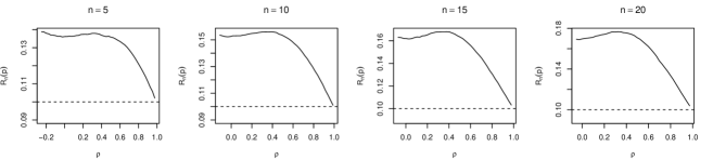
Figure 1: $R_{n}(p)$ for $n=5,10,15,20$, and $\rho\in[-1/(n-1),1]$ with $p=0.1$.

The second example presents the case of independent discrete uniform random variables on $\{1/m,\dots,m/m\}$, $m\geq 2$. Figure 2 gives $R_{n}(p)$ for $10$ discrete uniform random variables with different discretization $m$. We can see that as $m$ increases, $R_{n}(p)$ for discrete uniform random variables becomes closer to that for uniform random variables. Moreover, if $m$ is large, (14) holds for a wide range of $p$ in $(0,1)$ except for extremely small ones.

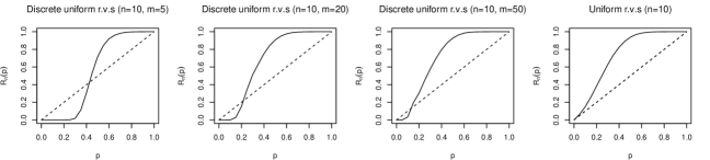
Figure 2: $R_{n}(p)$ for discrete p-values ($m=5,20,50$) and uniform p-values, with $p\in(0,1)$.

In Figure 3, we numerically compute the threshold $a_{n,p}$ of the harmonic mean p-value method for independent p-values and its asymptotic form (13). The thresholds are computed at significance levels $0.01$, $0.05$, and $0.1$, up to $5000$ p-values. The results suggest that the asymptotic threshold (13) can be a very good approximation of $a_{n,p}$ for large numbers of p-values. The numerical results are not stable for the case of $p=0.01$ and the plot is kinky.

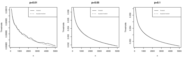
Figure 3: The asymptotic threshold (13) and $a_{n,p}$ of the harmonic mean p-value method for independent p-values.

7 Conclusion

Sub-uniformity of generalized means of standard uniform random variables $U_{1},\dots,U_{n}$ is studied under several dependence assumptions. In particular, sub-uniformity is shown to hold in three cases: (i) weak negative association (Proposition 4); (ii) the class of extremal mixture copulas (Theorem 1); (iii) some Clayton copulas (Theorem 2). These dependence structures can be used to construct a wide range of dependence structures for which sub-uniformity holds, as suggested by Propositions 2 and 3. Based on some numerical results, we conjecture that sub-uniformity also holds for Gaussian copulas with positive correlation coefficients. An important implication of sub-uniformity in multiple hypothesis testing is that merging p-values by any $r$-generalized mean function with $r\leq-1$ is anti-conservative across all significance levels in $(0,1)$. Although sub-uniformity cannot hold for discrete uniform random variables, using an $r$-generalized mean function with $r\leq-1$ can still be anti-conservative if the number of discretizations is large (Theorem 3). An asymptotic threshold of the harmonic mean p-value method for independent p-values is derived in Proposition 6. As the number of p-values increases, since the asymptotic threshold goes to 0, the harmonic mean p-value will be more anti-conservative if no adjustment is applied.

For the purpose of multiple testing under dependence, due to the anti-conservativeness results found in this paper, we recommend using the Simes method or the Cauchy combination, which are valid under independence and some other dependence assumptions, as well as their variants, over the harmonic mean p-value. Theorem 2 also gives a small threshold correction for the harmonic mean p-value under Clayton copulas, suggesting that the harmonic mean p-value may behave quite well under some forms of positive dependence.

We close the paper by noting that, although sub-uniformity can hold under a wide range of dependence structures of $U_{1},\dots,U_{n}$, there always exists some dependence structure under which sub-uniformity does not hold. For instance, since comonotonicity (i.e., $U_{1}=\dots=U_{n}$ almost surely) does not maximize the distribution function of the sum of random variables (see Wang et al. (2013) for bounds on the distribution function of the sum), it is always possible to construct a dependence structure of $U_{1},\dots,U_{n}$ such that $\mathbb{P}(w_{1}U_{1}^{r}+\dots+w_{n}U_{n}^{r}\leq t)>\mathbb{P}(U_{1}^{r}\leq t)$ for some threshold $t\in\mathbb{R}$ of interest. Therefore, conditions on dependence structures that lead to sub-uniformity or super-uniformity, other than the ones studied in this paper, require further research.

References

• Barber and Ramdas, (2017) Barber, R. F. and Ramdas, A. (2017). The p-filter: Multilayer false discovery rate control for grouped hypotheses. Journal of the Royal Statistical Society Series B (Statistical Methodology), 79(4), 1247–1268.
• Bates et al. (2023) Bates, S., Candès, E., Lei, L., Romano, Y. and Sesia, M. (2023). Testing for outliers with conformal p-values. Annals of Statistics, 51(1), 149–178.
• Block et al., (1982) Block, H. W., Savits, T. H. and Shaked, M. (1982). Some concepts of negative dependence. Annals of Probability, 10(3), 765–772.
• Block et al., (1985) Block, H. W., Savits, T. H. and Shaked, M. (1985). A concept of negative dependence using stochastic ordering. Statistics and Probability Letters, 3(2), 81–86.
• Chen and Sarkar, (2020) Chen, X. and Sarkar, S. K. (2020). On Benjamini–Hochberg procedure applied to mid p-values. Journal of Statistical Planning and Inference, 205, 34–45.
• Chen et al. (2024) Chen, Y., Embrechts, P. and Wang, R. (2024). An unexpected stochastic dominance: Pareto distributions, dependence, and diversification. Operations Research, forthcoming.
• Chen et al. (2023) Chen, Y., Liu, P., Tan, K. S. and Wang, R. (2023). Trade-off between validity and efficiency of merging p-values under arbitrary dependence. Statistica Sinica, 33(2), 851–872.
• Chi et al., (2022) Chi, Z., Ramdas, A. and Wang, R. (2022). Multiple testing under negative dependence. arXiv: 2212.09706.
• Dubey, (1970) Dubey, S. D. (1970). Compound Gamma, Beta and F distributions. Metrika, 16(1), 27–31.
• Embrechts and Puccetti (2020) Embrechts, P. and Puccetti, G. (2010). Risk aggregation. In Copula Theory and Its Applications (Eds: Jaworski, P. et al.), 111–126. Springer, Berlin, Heidelberg.
• Ferreira and Zwinderman, (2006) Ferreira, J. and Zwinderman, A. (2006). On the Benjamini–Hochberg method. Annals of Statistics, 34(4), 1827–1849.
• Fisher (1948) Fisher, R. A. (1948). Combining independent tests of significance. American Statistician, 2(30).
• Gui et al. (2023) Gui, L., Jiang, Y. and Wang, J. (2023). Aggregating dependent signals with heavy-tailed combination tests. arXiv: 2310.20460.
• Hardy et al. (1934) Hardy, G. H., Littlewood, J. E. and Pólya, G (1934). Inequalities. Cambridge University Press.
• Joag-Dev and Proschan (1983) Joag-Dev, K. and Proschan, F. (1983). Negative association of random variables with applications. Annals of Statistics, 11(1), 286–295.
• Lehmann (1966) Lehmann, E. L. (1966). Some concepts of dependence. Annals of Mathematical Statistics, 37(5), 1137–1153.
• Lin et al., (2024) Lin, L., Wang, R., Zhang, R. and Zhao, C. (2024). The checkerboard copula and dependence concepts. arXiv: 2404.15023.
• Lindley and Singpurwalla, (1986) Lindley, D. V. and Singpurwalla, N. D. (1986). Multivariate distributions for the life lengths of components of a system sharing a common environment. Journal of Applied Probability, 23(2), 418–431.
• Liu and Xie (2020) Liu, Y. and Xie, J. (2020). Cauchy combination test: A powerful test with analytic p-value calculation under arbitrary dependency structures. Journal of the American Statistical Association, 115(529), 393–402.
• McNeil et al. (2020) McNeil, A. J., Neslehova, J. G. and Smith, A. D. (2020). On attainability of Kendall’s tau matrices and concordance signatures. Journal of Multivariate Analysis, 191, 105033.
• Nelsen (2006) Nelsen, R. (2006). An Introduction to Copulas. Springer, New York, Second Edition.
• Ramdas et al. (2019) Ramdas, A. K., Barber, R. F., Wainwright, M. J. and Jordan, M. I. (2019). A unified treatment of multiple testing with prior knowledge using the p-filter. Annals of Statistics, 47(5), 2790–2821.
• Rubin-Delanchy et al., (2019) Rubin-Delanchy, P., Heard, N. A. and Lawson, D. J. (2019). Meta-analysis of mid-p-values: Some new results based on the convex order. Journal of the American Statistical Association, 114(527), 1105–1112.
• Samorodnitsky and Taqqu (1994) Samorodnitsky, G. and Taqqu, M. S. (1994). Stable Non-Gaussian Random Processes: Stochastic Models with Infinite Variance. Routledge.
• Samuel-Cahn, (1996) Samuel-Cahn, E. (1996). Is the Simes improved Bonferroni procedure conservative? Biometrika, 83(4), 928–933.
• Sarabia et al., (2016) Sarabia, J. M., Gómez-Déniz, E., Prieto, F. and Jordá, V. (2016). Risk aggregation in multivariate dependent pareto distributions. Insurance: Mathematics and Economics, 71, 154–163.
• Sarkar, (1998) Sarkar, S. K. (1998). Some probability inequalities for ordered MTP2 random variables: a proof of the Simes conjecture. Annals of Statistics, 26(2), 494–504.
• Shaked and Shanthikumar (2007) Shaked, M. and Shanthikumar, J. G. (2007). Stochastic Orders. Springer.
• Simes (1986) Simes, R. J. (1986). An improved Bonferroni procedure for multiple tests of significance. Biometrika, 73(3), 751–754.
• Vovk et al. (2005) Vovk, V., Gammerman, A. and Shafer, G. (2005). Algorithmic Learning in a Random World. Springer, New York.
• Vovk et al. (2022) Vovk, V., Wang, B. and Wang, R. (2022). Admissible ways of merging p-values under arbitrary dependence. Annals of Statistics, 50(1), 351–375.
• Vovk and Wang (2020) Vovk, V. and Wang, R. (2020). Combining p-values via averaging. Biometrika, 107(4), 791–808.
• Wang et al. (2013) Wang, R., Peng, L. and Yang, J. (2013). Bounds for the sum of dependent risks and worst Value-at-Risk with monotone marginal densities. Finance and Stochastics, 17(2), 395–417.
• Wilson (2019) Wilson, D. J. (2019). The harmonic mean p-value for combining dependent tests. Proceedings of the National Academy of Sciences, 116(4), 1195–1200.
• Xiong and Hu, (2022) Xiong, P. and Hu, T. (2022). On Samuel’s p-value model and the Simes test under dependence. Statistics and Probability Letters, 187, 109509.