Supersymmetric Expansion Algorithm and complete analytical solution for the Hulthén and anharmonic potentials
Abstract
An algorithm for providing analytical solutions to Schrödinger’s equation with non-exactly solvable potentials is elaborated. It represents a symbiosis between the logarithmic expansion method and the techniques of the superymmetric quantum mechanics as extended toward non shape invariant potentials. The complete solution to a given Hamiltonian is obtained from the nodeless states of the Hamiltonian and of a set of supersymmetric partners . The nodeless states (dubbed “edge” states) are unique and in general can be ground or excited states. They are solved using the logarithmic expansion which yields an infinite systems of coupled first order hierarchical differential equations, converted later into algebraic equations with recurrence relations which can be solved order by order. We formulate the aforementioned scheme, termed to as “Supersymmetric Expansion Algorithm” step by step and apply it to obtain for the first time the complete analytical solutions of the three dimensional Hulthén–, and the one-dimensional anharmonic oscillator potentials.
I Introduction
The Schrödinger equation occupies a pole position in the non-relativistic quantum mechanics as the knowledge of its solutions is the key prerequisite for carrying out all the analyses of the observable characteristics of quantum systems such as bound and continuous spectra, scattering cross sections, transition probabilities, electric and magnetic multipole moments etc. In its simplest version it describes two-body systems, such as the H Atom, di-atomic molecules etc. which allow for its reduction to a one-body problem. Due to the central symmetry of the majority of physics problems, it is often written in spherical polar coordinates and upon variable separation, the angular part is described by the spherical harmonics, while its radial part contains the potential. Among the potentials, those admitting exact solutions, i.e., solutions which can be cast in terms of elementary functions and termed to as Liouvillian SINGER1991251 , are of special interest as they often allow for realistic predictions of the physical properties of the systems under consideration, being the Coulomb problem of the H Atom the example of excellence. This part of quantum mechanics will be termed to as “Liouvillian Solvable Quantum Mechanics”.
Liouvillian Solvable Quantum Mechanics
Any potential in the Liouvillian Solvable Quantum Mechanics can be solved by subjecting the corresponding Schrödinger equation to a point-canonical transformation toward an exactly solvable second order differential equation of the type of the hyper-geometric-, Heun-, or other such equations R_De:1992 (see also Stevenson:1941 for earlier use of the method although not under the name of point-canonical transformation). As a rule, the solutions are exponentials times polynomials and their degrees, i.e. the numbers of nodes in the wave function constructed from them, are used as quantum numbers in the characterizations of the excited states. In Schrödinger’s work Schrodinger:1940xj , another scheme has been suggested for finding the solutions of exactly solvable potentials. The scheme is based on factorization of the Hamiltonian by two conjugate operators, the definition of the ground state as a function annihilated by one of them, and generation of the excited states by the repeated action on the ground state by the other operator. Schrödinger’s scheme culminated in the work by Infeld and Hull Infeld:1951mw who extended it to include a variety of potentials and thus established the factorization method in quantum mechanics.
Liouvillian Solvable SUSYQM
In the beginning of the 80ies Witten developed the idea about super-symmetric partner Hamiltonians Witten:1981nf which, in combination with the factorization method, lead to an efficient algebraic scheme for calculations of energies and eigenfunctions of all the known exactly solvable quantum mechanical potential problems. In the subsequent decade, the so called super-symmetric quantum mechanics (SUSYQM) experienced a period of extensive development and produced many remarkably results, among them the possibility of designing hierarchic chains constituted by partner Hamiltonians in such a way, that the ground state of the partner Hamiltonian is of same energy as the first excited state of the parent one, while the wave functions of the eigenstates to the two Hamiltonians are related by specific differential operators termed to as “intertwining”–, or, “shift” operators, a construct of many intriguing and useful properties. Compared to these activities, the quantum mechanical problems involving non-exactly solvable potentials, remained out of the main scope and the consensus has been that they have to be treated numerically and solved approximately by perturbative-, asymptotic iteration-, WKB and similar methods. In what follows we here term to this branch of quantum mechanics as “No Liouvillian Solvable Quantum Mechanics”.
No Liouvillian Solvable Quantum Mechanics
The potentials characterizing the No Liouvillian Quantum Mechanics are such that do not possess solutions which can be cast in terms of elementary functions, the simplest examples being polynomial potentials with arbitrary coefficients. Indeed, according to a theorem by Plesset Plesset:1932 , no exact solutions in terms of finite number of elementary functions can be found if the potential is a Laurent polynomial with arbitrary coefficients. In 1972 Hautot Hautot:1972 formulated conditions on the aforementioned coefficients which allowed to resolve the resulting polynomial potentials exactly. This work has been continued by Magyari Magyari:1981kx . The potentials conditioned in this way could be tackled equally well by the techniques of the Liouvillian solvable super-symmetric quantum mechanics Bera2017 and thus be incorporated into the latter.
Regarding unconditioned polynomial potentials, progress has been achieved by the so called expansion technique Bender:1988rq which solves the Schrödinger equation for a potential of the type, , for cases in which the exact solutions to are known. More specifically, first an artificial parameter is attached to , and then an expansion in this parameter is performed, which interpolates between the known potential for and the potential for . The expansion yields an infinite chain of coupled second order differential equations which can be solved order by order recursively. This scheme is especially suited for polynomial potentials with arbitrary coefficients such as anharmonic ones, in which case the coupled equations become algebraic and can be solved exactly, a reason for which such solutions are referred to as analytical. In this way, the no Liouvillian solutions can be obtained order by order with arbitrary accuracy. Examples can be found in Bera:2007 , Datta:2011zz .
In 1940, Bijl BIJL1940869 suggested to apply expansion techniques to the Schrödinger equation for the logarithm of the wave function, i.e. to represent as
| (1) |
In so doing one finds the following equation satisfied by ,
| (2) |
known as Riccati’s equation. Occasionally, (2) will also be referred to as “logarithmic form” of Schrödinger’s framework. Then an expansions in terms of an artificial parameter is performed
| (3) |
Back substituting the latter expansions into (2) amounts to an infinite chain of coupled, now first order differential equations which can be solved order by order recursively. This formalism acquired in Aharonov:1979gxt the name of Logarithmic Perturbation (also Logarithmic Expansion) technique. Similarly to the expansion technique, it again leads to solutions of arbitrary accurateness order by order. A difficulty of this method is the lack of well defined functions at the nodes of the wave functions, as they occur for excited states. Many authors from the late 70ies onward have updated and applied this method and found the energies and ground state wave functions to several anharmonic or exponential potentials (see Eletsky:1981fm and references therein as a representative example).
No Liouvillian Solvable SUSYQM
Non exactly or quasi-exactly solvable potentials play a crucial role in quantum mechanical problems. Among them such of wide spread refer
to anharmonic potentials and potentials containing centrifugal barriers which without the latter throughout might be exactly solvable. The
methods in the literature to tackle such problems are in their majority approximative, often based on perturbative or WKB approaches. Some
of them have been handled within the frameworks of the expansion techniques highlighted above.
In 1990 the expansion technique has been incorporated by Cooper and Roy into the framework of the super-symmetric quantum
mechanics in Cooper1990EF . As a reminder, the SUSYQM framework allows to produce the energies and wave functions in the
potential’s spectra by means of intertwining, i.e. shift operators and on the basis of the knowledge of ground states alone. In this fashion,
a new branch of the super-symmetric quantum mechanics, here termed to as “No Liouvillian solvable SUSYQM” arose in relation to
potentials with no-Liouvillian solutions, and in parallel to the Liouvillian Solvable SUSYQM, i.e. to the one devoted to potentials whose
solutions can be written in closed form.
Finally, in 2000 Lee demonstrated in LEE2000101 the equivalence of the logarithmic expansion technique and SUSYQM with an
incorporated expansion of the super-potential. Applications of this scheme can be found in Dhatt:2011 , where polynomial
potentials have been considered.
A full flashed consideration of an exponential potential (Yukawa’s, to be precise) in a new formalism for No-Liouvillian Solvable SUSYQM has been reported in Napsuciale:2020ehf ; Napsuciale:2021qtw . It is the goal of the present work to systematize and lift up the method employed in Napsuciale:2020ehf ; Napsuciale:2021qtw towards an algorithm applicable to a wide range of potentials of physical interest.
The layout of the work is as follows. In Section II we elaborate step by step on the new approach dubbed “Supersymmetric Expansion Algorithm (SEA)”, and explain how it incorporates several already known advances in the field next to new elements and allows us to solve some of the long pending potential problems. As a second example (after Yukawa’s potential) of the applicability of the SEA, in section III we use it to completely solve the three dimensional Hulthén potential. The complete analytical solution for the anharmonic potential and a proposal for a new supersymmetric formalism for perturbation theory are given in Section IV. The paper closes with concise conclusions in Section V.
II Supersymmetric Expansion Algorithm
The Schrödinger equation for a particle of mass in a one-dimensional potential is
| (4) |
The potential depends in general on parameters , related to the strength of the involved interactions or physical properties of the system. Each of these parameters defines a length scale , and we are free to single out one, to be denoted as , and associated with, say, the parameter , with the aim to write Schrödinger’s equation in terms of the dimensionless variable, , arriving at
| (5) |
with the following shorthand notations for the dimensionless quantities
| (6) |
A version of the Supersymmetric Expansion Algorithm (SEA) whose full systematic will be introduced in this work, was already employed to obtain for the first time a complete analytical solution to the Yukawa potential in Napsuciale:2020ehf ; Napsuciale:2021qtw . As it will be shown below, it can furthermore be applied to solve a wide class of potentials relevant in several branches of physics and chemistry and whose solutions have been considered as problematic so far, a reason for which we consider it worth of systematization. For the sake of simplicity in the notations from here onward we will consider only two parameters, and . The algorithm is summarized by the following ten steps:
-
1.
Use the typical scale dictated by the parameter to write the Schrödinger equation in terms of the dimensionless variable and the associated dimensionless quantities as
(7) Here we renamed to the parameter as it emerges upon the change of variable in (7). As this will turn out to be the first step in an iteration the procedure, to be described below, we attached a subscript ”” to all the quantities appearing at this stage. Within these notations, we are interested in the solutions to
(8) - 2.
-
3.
Expand the potential in powers of according to,
(11) and expand accordingly in(10) and the energy as
(12) -
4.
Re-design the product of the two infinite series defining the non-linear term in (9) as a single infinite series according to,
(13) Here, the coefficients are given by the following finite sums,
(14) Also note that
(15) does not involve .
-
5.
Use these elements in the logarithmic formulation of Schrödinger’s equation in (9) to obtain the infinite set of coupled first order differential equations
(16) (17) Explicitly, we find
(18) (19) (20) (21) (22) This is a cascade of linear differential equations, where the -th equation involves next to the solutions for . We can solve it starting from the equation for .
-
6.
For a wide class of potentials the coefficients are Laurent polynomials in , and one finds
(23) This expression includes both exponential and polynomial potentials, or any combination of them, among which those of highest importance are the potentials by Yukawa and Hulthén, the anharmonic potentials, not to forget the already solved Coulomb and harmonic oscillator potentials, in which case the solutions in for are polynomials,
(24) with being constant coefficients. The values of and depend on the potential and need to be worked out for each specific case. If we were able to solve the case in Eq.(16), then the remaining equations would become algebraic, and recurrence relations could be obtained for the coefficients and , obtaining order by order an analytical solution for the state and its eigenvalue .
In particular, if the potential is such that the solutions for are known, then the procedure outlined allows to obtain a solution for . This category includes but do not restrict to screening potentials and potentials of the form . The solution following from Eq. (10) reads
(25) where is a normalization factor. Notice that by construction, this solution has no nodes. This is an important point because we will show below that for some potentials relevant in physics and chemistry (e.g. screening potentials) this first solution corresponds to an excited state and in the past the main obstruction to the solution for excited states has been the assumed existence of nodes for all excited states.
The Hamiltonian can be factorized as
(26) with the factorization operators and being given by
(27) while the wave function is annihilated by as
(28) -
7.
The wave functions to the remaining states are then solved by the aid of techniques known from the supersymmetric quantum mechanics. One begins with constructing the first supersymmetric partner to as
(29) The associated potentials are then related by
(30) The superpartners and share same spectrum and have same number of states, except for one state, the “ground” state to . Indeed, suppose we find as an eigenstate to , i.e.
(31) Then
(32) therefore, is another eigenvalue of the with eigenstate .
-
8.
We apply the steps 2 to 6 to the partner Hamiltonian in order to obtain a solution to the Riccati equation for the corresponding super-potential , satisfying
(33) The solution so found yields the following nodeless eigenstate to
(34) It satisfies
(35) and yields, according to Step 7, a further solution to according to,
(36) This new solution to has nodes appearing due to the action of the operator on .
The Hamiltonian can now be factorized by itsef as
(37) where
(38) while the state satisfies
(39) -
9.
A further solution to can be obtained upon constructing the super-partner to , denoted by , and defined as
(40) The potentials are related as
(41) The corresponding superpotential satisfies
(42) which can be solved applying steps 2 to 6 now to to obtain the nodeless solution
(43) The corresponding eigenvalue is shared by both and , being the related eigenstates , and , respectively. These eigenstates have nodes generated by the action of and on the nodeless state respectively.
-
10.
We continue this process until we completely solve the original Hamiltonian . For each Hamiltonian , in the previous steps, the set of equations
(44) (45) becomes algebraic with a hierarchical structure, and recurrence relations can be obtained for the coefficients and , thus completely solving the problem.
We remark that only few of the eigenvalues and eigenstates of the Hamiltonian we are interested in, , are directly obtained by applying to it the logarithmic formalism and the expansion of the potential, in a way that yields a nodeless solution. The remaining eigenstates and eigenvalues of are indirectly obtained solving first the supersymmetric partners (which yields the common eigenvalue) and applying the factorization operators on these (also nodeless) solutions. In each step increasing , we obtain a nodeless solution of which upon the action of the factorization operators yields an eigenstate of in the form of a polynomial times the nodeless eigenstate. It is clear that the solution is build up on the initial nodeless solutions of and the superpartners . It is a wide spread belief that for any Hamiltonian the only nodeless state is the ground state. We find that this not generally true, and there exist nodeless excited states which in our formalism are instrumental in solving the problem. For this reason, we single out these states and dub them edge states. The name comes from the extremal values that these states have for the angular momentum quantum number in the case of screening potential, but in general edge states can be defined as nodeless (excited or ground) states.
The Supersymmetric Expansion Algorithm combines several achievements in the literature, to be listed below, and also adds some new elements to yield a quite a robust framework. Steps 2-5 resemble the formalism of the Logarithmic Perturbation Theory (LPT) developed for the calculation of perturbative corrections to the ground states of several potentials in an formalism alternative to the Rayleigh-Schrödinger (RS) theory. In Refs. Aharonov:1979gxt Dolgov:1978bc relations analogous to Eqs.(16,17) were obtained for perturbed ground states, which were solved using as integrating factor unperturbed ground states. The corrections to arbitrary order were obtained in the form of integrals over the whole space involving the ground state probability function, the perturbation potential, and the lowest order corrections . Correction to excited states, expanded in powers of the perturbation parameter, were calculated by writing them as a products of the ground state, cast into an exponential form, and a polynomial, containing the nodes of the perturbed states. At this point the calculation becomes cumbersome and its efficiency with respect to the RS formalism gets lost. There have been several attempts in the literature to avoid the problem with handling the nodes of the excited states, a difficulty which limits applications of the logarithmic expansion method (see Bandyopadhyay:2002 and references therein for alternatives).
The same idea was applied to solve for the ground state of the screened coulomb potential in Eletsky:1981fm Vainberg:1981 where it could be shown that Eqs.(16,17) have polynomial solutions. The logarithmic perturbation theory (LPT) could be applied to the aforementioned ground state only because it was nodeless, and could well be defined in this case. In the present work we will show below how excited states with nodes, associated with a principle quantum number , can be build up from the only nodeless excited state (the “edge” state) through the action on it by the factorization operators of supersymmetry. In this fashion, the logarithmic expansion method, once supplemented by the technique of the supersymmetric quantum mechanics, allows to avoid the old problem of nodes in the excited states. A similar option has already been considered in LEE2000101 , where a comparison of LPT with SUSY quantum mechanics, combined with a -expansion a la Bender:1988rq of the superpotential has been undertaken.
Another related development is the use of SUSY for a restricted class of potentials which have the property dubbed ”shape invariance” Gendenshtein:1984vs . In this case, the super-partner generated in steps 7 to 10 belongs to the same family of Hamiltonians differing only by a function of the parameter . The harmonic oscillator and Coulomb potentials belong to this category. In this case it is possible to obtain straightforwardly the whole set of eigenvalues and eigenfunctions in closed forms. Shape invariance is a property of supersymmetric Hamiltonians which are factorizable as defined in Ref. Infeld:1951mw . In the SEA formalism, are a chain of SUSY partners although shape invariance is not at all required, thus extending the field for applications of the techniques of supersymmetric quantum mechanics.
Closely related to the present work is the one in Dhatt:2011 , where a formalism for perturbation theory is proposed for potentials of the form . Polynomial solutions are assumed and the ground state is also solved using the expansion for the superpotential in the ground state. The problems of the nodes is avoided by constructing supersymmetric partner potentials which are directly and recursively written starting with the super-potential for the ground state. In this manner, the set of potentials are constructed and the excited states are obtained acting successively with intertwining operators on the ground states of ’s. The super-partners are solved using similar expansions for their own ground states. There are, however, several striking differences with our formalism. Firstly, the scheme in Dhatt:2011 is designed for a perturbative calculation. This is not the case of our SEA framework, although it can also be used for such purposes. Secondly, the assumption of polynomial solutions for the super-potentials works only for polynomial perturbations. Finally, but even more important, the aforementioned scheme is designed to start the sequence by the ground state. This is convenient for unperturbed potentials, as is the harmonic oscillator, used in the examples worked out there. In our SEA framework, we show instead that in general it is possible to start the iterative procedure with a properly chosen excited state (the edge state), which enlarges the applicability of our method.
III Supersymmetric Expansion Algorithm at work: Hulthén potential
The Supersymmetric Expansion Algorithm was employed in Napsuciale:2020ehf ; Napsuciale:2021qtw to obtain a complete analytical solution for the Yukawa potential 111The convention for and operators used in Napsuciale:2020ehf ; Napsuciale:2021qtw is exchanged here to match the more common convention in the literature for these operators.. In this section we will apply it to completely solve the Hulthén potential, giving more details on the derivation of the algebraic solution via the recurrence relations, which have not not been presented in Napsuciale:2020ehf ; Napsuciale:2021qtw .
Proposed originally to describe nuclear interactions, the Hulthén potential Hulthen:1942 finds applications in atomic-, Tietz:1961 ; Lai:1980 , solid-state– Berezin:1986 , and chemical physics Pyyokko:1975 . Exact solutions have been reported only for the states Lam:1971 ; Flugge:1999 . Approximate solutions for the states have been obtained using a variety of methods Lai:1980 ; Patil:1984 ; Roy:1987 ; Gonul:2000kix . Results on the numerical solutions as well as a comparison with previous approximate results can be found in Ref. Varshni:1990zz . To the best of our knowledge, the complete analytical solutions to Schrödinger’s equation with this potential are still missing and it is our goal here to fill this gap upon applying the SEA framework described in the previous section.
The Hulthén potential is given by
| (46) |
The typical distance scale for the Hulthén potential associated to the coupling is given by . Using this scale, the dimensionless potential can be written in either one of the following three forms,
| (47) |
where . We need to solve the Schrödinger equation (7) for the effective dimensionless potential and energy given by
| (48) |
The potential allows for the following expansion,
| (49) |
with the Bernoulli’s numbers being,
| (50) |
This expression yields the following expansion coefficients,
| (53) |
where
| (54) |
The set of equations (16,17) in this case reads
| (55) | ||||
| (56) |
The solutions up to are given by
| (57) | ||||||
| (58) | ||||||
| (59) | ||||||
| (60) | ||||||
| (61) | ||||||
| (62) |
where . We can see here that for the solutions for the expansion coefficients of the superpotential are of the form
| (63) |
However, we obtain more information from the solutions of the first few terms which is crucial for the formalism. Indeed, the leading term in the Hulthén potential corresponds to the Coulomb potential which has energies , thus solutions to the Hulthén potential can also be labelled by a principal quantum number in addition to the angular momentum and our formalism at this point yields the solution for . The solution to the Riccati equation in this step reads
| (64) |
where is arbitrary and we have the first six terms of in Eq. (12). At this point, it is convenient to separate the -independent contribution and to write
| (65) |
where
| (66) |
The solution can be rewritten as
| (67) |
with
| (68) |
Notice that for the solution in Eq.(67) describes an excited state. This sounds strange on the light of the widely spread belief that all the excited states have nodes and the logarithmic formulation cannot be applied to them because the logarithm is ill-defined at the nodes. We can see explicitly in Eq. (67) however, that the state has multiple zeroes at which is an end point, thus strictly speaking these states have no nodes and can be obtained using the logarithmic formalism.
For a given , the state is the only state with this property and we single it out, dubbing it edge state within the level, this because it corresponds to the maximal value.
There is an edge state for every level and all the states are given by Eq.(67) with the different values of distinguishing them. Notice also that there exist edge states for every potential in the calculation at a given order . In particular, we have nodeless excited states for every level in the Coulomb case which corresponds to the calculation to order with .
The edge states will be the starting point to solve the remaining states with . Since is arbitrary the procedure yields the complete solution for the Hulthén potential. With this aim, we insert the expansion (63) in Eqs. (56), for to get
| (69) |
where
| (70) |
which yields the following recurrence relations:
| (71) | ||||||
| (72) | ||||||
| (73) | ||||||
| (74) | ||||||
The coefficients include products of with , which in the -step are already known, thus, these recurrence relations completely solve the problem for the edge state in Eq.(67) with
| (75) |
Now we continue with the steps 7-8 in the SEA. The first partner potential is given by
| (76) |
The coefficients for
| (77) |
are polynomials in . We solve this potential in a similar way as . Expanding the superpotential ) and the energy , the Riccati equation for yields for
| (78) |
while for produces the cascade of equations
| (79) |
Expanding now
| (80) |
and inserting the expansion in Eq.(79) amounts to
| (81) |
where
| (82) |
We obtain the following recurrence relations,
| (83) | ||||||
| (84) | ||||||
| (85) | ||||||
| (86) | ||||||
These recurrence relations completely solve the problem for . Notice that is different from but it is also a screening Hamiltonian in the sense that it reduces to the Coulomb Hamiltonian in the limit. This allows us to identify the eigenstate, here denoted by , of the leading term of (though not of ) as a -state. Explicitly, it is given by
| (87) |
where we from here onward skip normalization factors. The function in the exponential is now given by
| (88) |
As already emphasized above, is an edge state for , but not an eigenstate of . However, due to supersymmetry, belongs to the spectrum of with eigenstate
| (89) |
Using Eq.(27) it is easy to check that this state has multiple nodes.
Notice that the recurrence relations for in Eqs. (83-86) are quite similar to those of in Eqs. (71-74). The former can be obtained from the latter by the replacement everywhere and adding the term to the relations for . These changes reflect the effects of the term in the partner potential in Eq.(76).
In Step 9 of the SEA framework, we construct and solve by the same method the superpartner to , denoted as , whose potential is
| (90) |
For the leading Coulomb term we find
| (91) |
while for we encounter the following recurrence relations:
| (92) | ||||||
| (93) | ||||||
| (94) | ||||||
| (95) | ||||||
They yield the solution for the edge eigenstate of as
| (96) |
where
| (97) |
The eigenvalue is a common eigenstate of and the eigenstates to and and given in their turn as
| (98) | ||||
| (99) |
Finally, in Step 10, the solution to is obtained in a similar way. For we find
| (100) |
while for we encounter the following recurrence relations:
| (101) | ||||||
| (102) | ||||||
| (103) | ||||||
| (104) | ||||||
They yield the complete solution for the edge eigenstate of , given by
| (105) |
where
| (106) |
This is not an eigenstate to but supersymmetry connects the chain of Hamiltonians , thus making a common eigenvalue. The corresponding eigenstate of is given by
| (107) |
The procedure terminates for with reaching and solving for the edge eigenstate state to , which then yields the solution of the Hulthén potential as
| (108) |
In our calculation we skipped normalization factors for the sake of simplicity, so at the end every state needs to be properly normalized.
Summarizing this long calculation, the eigenstates and eigenvalues for the Hulthén potential are given by
| (109) | ||||
| (110) |
where .
Our procedure is graphically illustrated in Fig. 1 for the solution of the level , where we use the notation . We first solve the Riccati equation for using the expansion of the potential , to find the energy and superpotential . The obtained solution corresponds to the edge state. Then we use supersymmetry to build and solve likewise the superpartner , whose edge state turns out to be . The eigenstate of of our interest, is obtained by the action of the operator on . The remaining states for are obtained constructing likewise the super-partner Hamiltonians , solving them by the same procedure, which yields the respective edge states. The eigenstates of are obtained by the successive action of the factorization operators on the former states. In this manner, we solve completely for all the eigenstates of in the level. The same procedure is applied to every level to achieve the complete analytical solution for the Hulthén potential.
It is important to emphasize that, unlike the Coulomb case, for the Hulthén potential the supersymmetric Hamiltonians do not constitute a family of shape invariant potentials, i.e., they can not be related to each other just by a parameter change. A similar observation has been reported regarding the Yukawa potential in Napsuciale:2020ehf ; Napsuciale:2021qtw . There, the property of shape invariance was lost already beyond the order of in the potential’s expansion. Shape invariance is a powerful property in the Liouvillian solvable SUSYQM, but it is not required by the No Liouvillian solvable one, which is our case. Stated differently, our formalism goes beyond shape invariance and thus makes use of the full power of supersymmetry. It is also worth mentioning that as a byproduct of the aforementioned calculation the complete analytical solutions of all the members of the chain of supersymmetric Hamiltonians were obtained, not only those of the genuine Hulthén Hamiltonian . Furthermore, the calculation at a given order yields the complete exact solution of the expansion of any one of the Hamiltonians in the chain to this order. Therefore, we actually could obtain systematically the analytical solutions to an infinite set of Hamiltonians , . Similar considerations apply to the supersymmetric Hamiltonians to any arbitrary potential solved by the SEA approach.
The results for the energy levels in Eq.(110) can be written in terms of and . It turns out that they depend only on and according to
| (111) |
The coefficients have long expressions for large thus we list them here only up to
| (112) | ||||
| (113) | ||||
| (114) | ||||
| (115) | ||||
| (116) | ||||
| (117) | ||||
| (118) | ||||
| (119) | ||||
| (120) | ||||
| (121) | ||||
| (122) |
Notice that all the coefficients for odd vanish and for the even coefficients are proportional to thus, for the states the contributions beyond are nule and the energy levels gain the exact form
| (123) |
This result has been previously obtained in Lam:1971 ; Flugge:1999 where a closed solution for the states is given. It is interesting to explicitly obtain the closed solutions in this case, since our power series solution must correspond to these closed form solutions in this particular case. Following Lam:1971 we write
| (124) |
where is a free parameter. The Schrödinger equation for states yields the following equation for
| (125) |
Changing variable to gives
| (126) |
This equation simplifies with the choice
| (127) |
which yields
| (128) |
Expanding in powers of
| (129) |
and inserting this series in Eq. (128) gives together with the following recurrence relations for :
| (130) |
Obviously, the series diverges for , and one can find solutions only if nullifies for some , in which case a quantization condition is obtained as
| (131) |
Thus, the energy levels for the states of the Hulthén potential are obtained as
| (132) |
The explicit form of the states in terms of are then found as
| (133) |
where are polynomials in of degree . These solutions are normalizable only for . The polynomials for the normalized ground and first excited states read:
| (134) | ||||
| (135) |
In terms of the variable we find
| (136) | ||||
| (137) |
Expanding the states in powers of , the series obtained within the SEA framework are recovered. This can be straightforwardly verified for the ground state at the level of the logarithmic form of Schrödinger’s equation for ,
| (138) |
solved by
| (139) |
The expansion then coincides with our solution in Eq(65) for the case . The complete solution to the Hulthén potential obtained here includes the results in Lam:1971 ; Flugge:1999 for the states and also the results obtained in Lai:1980 for arbitrary .
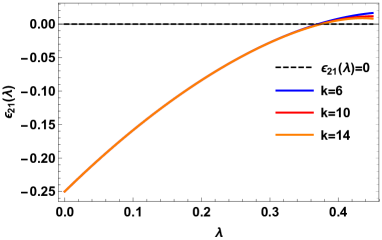
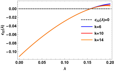
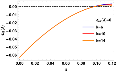
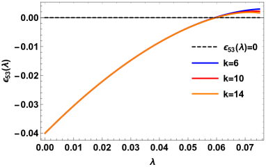
In Fig. 2 we plot for and , considering the expansions up to with . We can see that the series are convergent in the whole range of values of where bound states exist, i.e., below the critical value where . Similar results are obtained for all the levels.
Using the expansion up to we estimate the critical values with an accuracy at the percent level. More precise results can be obtained if we reconstruct the function using methods like the Padé approximants. In Table 1 we list the precise results for the critical screening lengths obtained from the and Padé approximants (which requires to calculate the Taylor series of up to ). The uncertainty in the calculation is taken from the difference in the result obtained using the and Padé approximants.
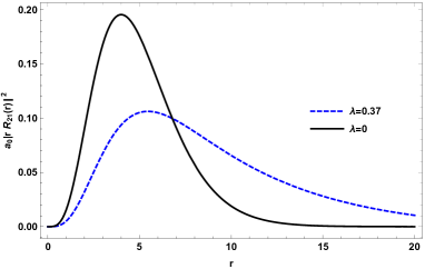
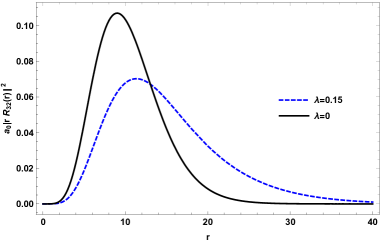
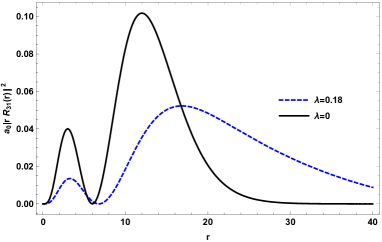
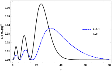
As to the eigenstates, in Fig. 3 we plot the radial probabilities for the lowest lying calculated with the Padé approximant for values of close to the critical values, together with the Coulomb probabilities. We can see in these plots the beginning of the delocalization of the states for close to the critical values, even though the peaks in the radial probability are only slightly shifted towards larger radius, the shift being more pronounced for excited states with low values of .
| 1 | 0 | 2 |
| 2 | 0 | 1/2 |
| 2 | 1 | 0.3767388(1) |
| 3 | 0 | 2/9 |
| 3 | 1 | 0.18638519(1) |
| 3 | 2 | 0.1576540(1) |
| 4 | 0 | 1/8 |
| 4 | 1 | 0.11042423(5) |
| 4 | 2 | 0.09755514(4) |
| 4 | 3 | 0.08640416(2) |
| 5 | 0 | 2/25 |
| 5 | 1 | 0.07281399(4) |
| 5 | 2 | 0.06609952(3) |
| 5 | 3 | 0.05997137(1) |
| 5 | 4 | 0.054505130(5) |
| 6 | 0 | 1/18 |
| 6 | 1 | 0.05154187(2) |
| 6 | 2 | 0.04765376(2) |
| 6 | 3 | 0.04397303(1) |
| 6 | 4 | 0.040584332(5) |
| 6 | 5 | 0.037504108(2) |
| 7 | 0 | 2/49 |
| 7 | 1 | 0.03836901(2) |
| 7 | 2 | 0.03594088(1) |
| 7 | 3 | 0.033579387(7) |
| 7 | 4 | 0.031352334(4) |
| 7 | 5 | 0.029284146(2) |
| 7 | 6 | 0.027378996(1) |
| 8 | 0 | 1/32 |
| 8 | 1 | 0.02965680(2) |
| 8 | 2 | 0.02805166(1) |
| 8 | 3 | 0.02645746(1) |
| 8 | 4 | 0.024925430(3) |
| 8 | 5 | 0.023478153(2) |
| 8 | 6 | 0.022124095(1) |
| 8 | 7 | 0.0208642596(4) |
| 9 | 0 | 2/81 |
| 9 | 1 | 0.02360076(1) |
| 9 | 2 | 0.02249094(1) |
| 9 | 3 | 0.021370275(5) |
| 9 | 4 | 0.020276903(3) |
| 9 | 5 | 0.019229555(2) |
| 9 | 6 | 0.018237044(1) |
| 9 | 7 | 0.0173026475(5) |
| 9 | 8 | 0.0164264743(2) |
We will release with the published version of this paper a freely available code for the solution of the recurrence relations which provides the solutions for the energy levels and normalized eigenstates to the desired order , along with some details of the phenomenology for the Hulthén potential.
IV One dimensional anharmonic oscillator potential within the SEA approach and perturbation theory
IV.1 Anharmonic oscillator potential
Every physical systems behave like harmonic oscillators for small motion around given equilibrium points, characterized by local minima in the corresponding potentials. For parity invariant interactions, the leading correction to this simple behavior is the anharmonic potential which, for a one-dimensional system, has the form of . The calculation of the corrections to the energy levels is of a primary concern for several branches of natural sciences and in the past there have been many attempts to solve this problem. The analytic structure of the ground state energy using the WKB approximation and the calculation of the Taylor series for the Rayleig-Schrödinger anharmonic corrections for this level have been reported by Bender:1969si up to the very high order () in the perturbation theory, definitively knotting though on diverging series. A rigorous derivation of the analytic structure of the ground state energy and the asymptotic behavior at were given in Simon:1970mc , where the asymptotic nature of the series was established. Precise results for this level were given also in Loeffel:1969rdm , where a reconstruction of the ground state energy was performed employing the Padé approximant, with the coefficients of the Taylor series found in Bender:1969si . For other techniques for obtaining approximate solutions to the anharmonic oscillator for the ground and excited states see Hioe:1978jj ; Amore:2004 and references there in. Upper and lower bounds on the actual values of the first energy levels have been set in Bazley:1961 . Moreover, the ground state energy for the -dimensional harmonic oscillator and the corresponding anharmonic corrections up to the order of to it as following from the LPT framework, have been worked out in Dolgov:1979hv . In summary, though one can find approximate calculations of the anharmonic corrections to the harmonic oscillator, a systematic complete solution still seems to be an open problem. In the following we will make use of the supersymmetric expansion algorithm to provide such a solution.
The one-dimensional anharmonic potential reads
| (140) |
Using the typical scale of the leading harmonic oscillator term, we obtain
| (141) |
where . We can view this potential as a power expansion in with the coefficients
| (145) |
The cascade of equations for in this case emerges as
| (146) | ||||||
| (147) | ||||||
| (148) |
These equations have polynomial solutions which can be easily worked out. In particular, the solutions up to are
| (149) | ||||||
| (150) | ||||||
| (151) | ||||||
| (152) | ||||||
| (153) | ||||||
| (154) |
These results suggest that the coefficients in the expansion of the the super-potential for the first solution to are of the form
| (155) |
Inserting Eq.(155) in Eq. (148), we find that for , the coefficients vanish for even , and for odd they satisfy the following recurrence relations
| (156) |
while for and for the energy coefficients we obtain
| (157) | ||||
| (158) |
Skipping normalization factors, the first solution to will be
| (159) |
where
| (160) |
Similarly to the Hulthén’s potential case, we get more information from the first few terms in the expansion in for this solution. Indeed, the leading term () corresponds to the ground state of the harmonic oscillator, thus this solution is the ground state of . We conclude that, unlike the case of the screening potentials, the anharmonic Hamiltonian has only one nodeless state and it is the ground state .
The calculation of the excited states requires to construct the set of supersymmetric partners . We skip the details of the by now familiar calculations and present only the results for the recurrence relations of . The coefficients in the expansion of the the super-potential for are of the form
| (161) |
For the solutions are given by
| (162) | ||||||
| (163) |
For , the coefficients also vanish for even and for odd they satisfy the following recurrence relations
| (164) |
while for and for the energy coefficients we obtain
| (165) | ||||
| (166) |
The solution to is given by
| (167) |
where
| (168) |
Notice that the -independent energy levels in Eq.(162) correspond to the eigenvalues of the harmonic oscillator, thus we identify as the conventional quantum number of the harmonic oscillator. The solution for the only nodeless state of (the ground state for this Hamiltonian), , provides a new solution to every previously constructed superpartner in the set which is an excited state and is obtained by the successive action of factorization operators on . In particular, for the anharmonic Hamiltonian the new unnormalized solution reads
| (169) |
We remark that continuing this process we construct the solutions for the infinite set of superpartners . Furthermore, this solution is valid when we work at a finite order in the expansion in , thus our procedure yields the solution to an infinite set of Hamiltonians at every order .
In summary, the energy for the -th level of the anharmonic oscillator can be written as
| (170) |
while the unnormalized eigenstates are given by
| (171) |
where
| (172) |
is the nodeless solution (ground state) of the supersymmetric with
| (173) |
Below we list only the first ten coefficients because of the large expressions
| (174) | ||||
| (175) | ||||
| (176) | ||||
| (177) | ||||
| (178) | ||||
| (179) | ||||
| (180) | ||||
| (181) | ||||
| (182) | ||||
| (183) | ||||
| (184) |
The scheme of this calculation can be graphically illustrated similar to Fig. 4 where we use the notation for the eigenstate corresponding to the level of the Hamiltonian and we show the solution up to the level. First we use the logarithmic expansion to solve obtaining in this case the solution to the ground state which is the only edge state for the anharmonic potential. Then, we construct the superpartner and solve it by the same method. The solution, , is the only edge state for and turns out to be its ground state. This solution provides the solution for the first excited state, , of obtained by the action of on . Next we construct the superpartner , solve it likewise and from the obtained solution for its unique edge state, , which turns out to be its own ground state, we obtain the first excited solution of by the action of on and the second excited state of of our interest, , acting with on . The procedure is similar for the calculation of higher excited states of the anharmonic Hamiltonian . Notice that the supersymmetric structure here is different to the Hulthén or Yukawa case where every superpartner has an edge state for every level. For the anharmonic case, every superpartner has only one edge state which corresponds to its own ground state as expected from the conventional realization of supersymmetry.
As a result of the anharmonic term, the levels are now dependent and not equally spaced, the separation of the levels depending on the specific value of . The simplicity of the harmonic oscillator is completely lost and the shape invariance property of the harmonic oscillator is lost already at order .
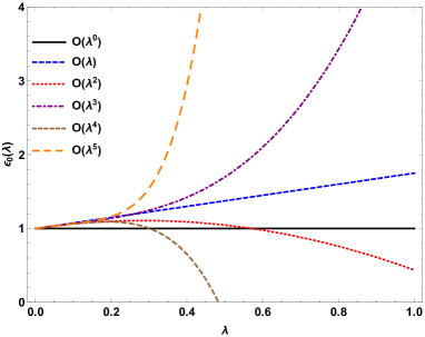
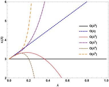
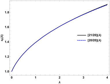
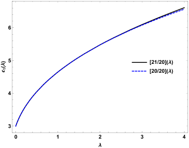
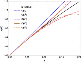
For the ground energy () of the coefficients reproduce those of Ref.Bender:1969si (the coefficients used in the expansion of the ground energy there are related to our coefficients as ). There are large coefficients in the expressions for and the series seems convergent at most for very small values of . In Fig. 5 we plot the ground energy and the first excited state calculated to for , where we can see that the series diverges beyond the very small region. The functions can be reconstructed using techniques like the Padé approximants. The figure 5 is illustrative of the reconstruction of and using the and approximation, which requires to calculate the series up to . The actual value of the functions lies between these approximants and we can estimate the uncertainty in the reconstruction from the difference between them for a given value. Even for values as large as , we obtain a precision of one part per thousand in the calculation of these energy levels.
Our results show that because of the poor convergence of the series, care is in order regarding perturbative calculations in anharmonic theories. The potential is used in the standard model, where the Higgs coupling has the tree level value . Using GeV and GeV we get . Our quantum mechanical calculations can be considered as calculations in a one-dimensional quantum field theory and in this simple scenario we can check the usefulness of the perturbative expansion for this value of . In Fig. 6 we show the ground energy for small calculated in a perturbative scheme up to , as well as the energy function reconstructed with the Padé approximant. It is clear here, that for the perturbative calculation up to order yields results approaching the actual value of the energy function, although at order the calculation does not improve that much. Moreover, at the order of the calculation definitively yields the same precision as the calculation to the order of . The perturbative expansion breaks at for and higher order terms beyond this point are useful only for the reconstruction of the ground energy using techniques like the Padé approximant. This is a one-dimensional field theory result and it would be interesting to explore if these results persist for physical four-dimensional theories, which is beyond the scope of this work.
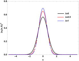
As to the probability distributions, the calculation of the series has also a poor convergence, but calculating enough terms in the series we can confidently reconstruct the wave functions for large values of . In Fig. 7 we show the probability for the ground state as reconstructed with the Padé approximant. We can see that the shape of this function is similar to the one of the harmonic oscillator (), and that with the increase of , the probability becomes more compact around the origin. Similar results are obtained for the excited states.
IV.2 Supersymmetric perturbation theory
The case of the anharmonic potential shows that the SEA approach allows to completely solve a problem that has been considered in the past using Rayleigh-Schrödinger perturbation theory, with being considered as a small perturbation of the well known solution of the harmonic oscillator. There is nothing technically special in the harmonic oscillator and we can start with any potential with known solutions and apply the formalism for a general perturbation . Indeed, let us consider the general problem of the potential
| (185) |
where the solutions to are known. Using the length scale associated with , the Schrodinger equation is reduced to
| (186) |
We search for the solutions of
| (187) |
where
| (188) |
This potential can be written as
| (189) |
where
| (193) |
Following the steps prescribed by the SEA framework, the cascade of equations for the coefficients in the expansion in is produced as
| (194) | ||||||
| (195) | ||||||
| (196) |
The solutions to Eq.(194) are known and, in cases when the perturbation is a polynomial in (which covers most of the cases of physical interest), we can solve this cascade of equations for the edge states at the desired order, thus obtaining easily results which have been cumbersome to calculate in the conventional Rayleigh-Schrödinger perturbation theory. For other states we can construct the set of supersymmetric partners or even apply the steps in the SEA to completely solve this problem if necessary.
V Conclusions
In this work we elaborated a Supersymmetric Expansion Algorithm for obtaining analytical solutions to non-exactly solvable quantum potential problems. The method incorporates previous achievements in the literature, such as the combination of the logarithmic expansion method and the supersymmetric quantum mechanics, next to new elements, such as the concept of “edge” states, to produce a robust framework, applicable to a wide class of potentials. Contrary to common belief, we find that for some physical systems of interest (notoriously screened potentials), there exist unique excited states which have no nodes. We call them “edge” states (excited or ground) and are a new element of the No Liouvillian solvable SUSYQM. In the Liouvillian solvable SUSYQM, the “edge” states correspond to the ground states of the supersymmetric partners in the hierarchy chain.
The algorithm uses the logarithmic expansion to solve all the edge states of the system and of the auxiliary supersymmetric partners required to completely solve the problem. The procedure avoids the old problems with the nodes in the calculation of the excited states, solving first the edge states of the supersymmetric set of Hamiltonians and obtaining then the excited states of the system upon the application of the factorization operators of supersymmetry on the solutions for the edge states.
The expansions in series of the ingredients of Schrödinger’s equation, such as energies, wave functions, potentials, and super-potentials, produce infinite sets of coupled first order differential equations which can be reduced to hierarchical algebraic equations for the coefficients in the expansion and solved exactly order by order, thus providing analytical solutions. Along these lines, the three dimensional Hulthén potential, and the one dimensional anharmonic oscillator potentials could be completely resolved. For Hulthén’s potential, the solutions present themselves as infinite series in the screening length. For zero angular momentum our series reduce to the series expansions of the exact solutions, previously worked out in Lam:1971 ; Flugge:1999 . We obtain for the first time in the literature, power series solutions for the remaining states. The power series solutions are convergent for screening lengths below the critical values. We provide precise values for the critical values of the screening for all energy levels up to using the power series expansion up to order and reconstructing the energy functions with Padé approximants.
The power series solutions to the anharmonic potential have a poor convergence, though we could reconstruct the energies as functions of at the desired precision level using Padé approximants. We find that even for small values, as the value of the quartic coupling of the Higgs model in the standard model, , the perturbative scheme breaks down already at . The eigenstates have a similar form as those of the harmonic oscillator, although they are more compact. The nodes of the excited states are shifted to the equilibrium position .
These two examples of long pending unsolved potentials, present just a small illustration of the predictive power of the Supersymmetric Expansion Algorithm which can be employed for many other purposes, specially as an efficient tool for perturbative calculations. It is not the aim of this paper to analyze in detail the phenomenology of the numerous applications the two potentials here considered enjoy in physics and chemistry. We limited ourselves to generate the solutions which can be used for such purposes and, for this sake, we will provide freely available codes for the Hulthén and anharmonic potentials in the published version of this paper, solving the algebraic recurrence relations which give automatically the solutions to the desired order alongside with some phenomenology of the eigenstates and eigenvalues.
References
- (1) M. F. Singer, Liouvillian solutions of linear differential equations with Liouvillian coefficients, Journal of Symbolic Computation 11 (1991) 251.
- (2) R. De, R. Dutt and U. Sukhatme, Mapping of shape invariant potentials under point canonical transformations, Journal of Physics A: Mathematical and General 25 (1992) L843.
- (3) A. F. Stevenson, Note on the ”Kepler problem” in a spherical space, and the factorization method of solving eigenvalue problems, Phys. Rev. 59 (1941) 842.
- (4) Schrödinger, Erwin, A method of determining quantum-mechanical eigenvalues and eigenfunctions, Proc. Roy. Irish Acad. A 46 (1940) 9.
- (5) L. Infeld and T. Hull, The factorization method, Rev. Mod. Phys. 23 (1951) 21.
- (6) E. Witten, Dynamical breaking of supersymmetry, Nucl. Phys. B 185 (1981) 513.
- (7) M. S. Plesset, The Dirac electron in simple fields, Phys. Rev. 41 (1932) 278.
- (8) A. Hautot, Schrödinger’s equation and special radial electric fields, Physics Letters A 38 (1972) 305.
- (9) E. Magyari, Exact quantum mechanical solutions for anharmonic oscillators, Phys. Lett. A 81 (1981) 116.
- (10) S. Bera, B. Chakrabarti and T. K. Das, Application of conditional shape invariance symmetry to obtain the eigen-spectrum of the mixed potential , Physics Letters A 381 (2017) 1356.
- (11) C. M. Bender, K. A. Milton, M. Moshe, S. S. Pinsky and L. M. Simmons, Jr., Novel Perturbative Scheme in Quantum Field Theory, Phys. Rev. D 37 (1988) 1472.
- (12) D. J. Bera, P.K., Linear delta expansion technique for the solution of anharmonic oscillations, Pramana 68 (2007) 117.
- (13) J. Datta and P. K. Bera, Iterative approach for the eigenvalue problems, Pramana 76 (2011) 47.
- (14) A. Bijl, The lowest wave function of the symmetrical many particles system, Physica 7 (1940) 869.
- (15) Y. Aharonov and C. K. Au, New approach to perturbation theory, Phys. Rev. Lett. 42 (1979) 1582.
- (16) V. Eletsky, V. Popov and V. Weinberg, Logarithmic perturbation theory for the screened coulomb potential, Phys. Lett. A 84 (1981) 235.
- (17) F. Cooper and P. Roy, -expansion for the superpotential, Physics Letters A 143 (1990) 202.
- (18) C. Lee, Equivalence of logarithmic perturbation theory and expansion of the superpotential in supersymmetric quantum mechanics, Physics Letters A 267 (2000) 101.
- (19) S. Dhatt and K. Bhattacharyya, Concurrent multiple-state analytic perturbation theory via supersymmetry, Journal of Mathematical Physics 52 (2011) 042101 [https://pubs.aip.org/aip/jmp/article-pdf/doi/10.1063/1.3570817/14750710/042101_1_online.pdf].
- (20) M. Napsuciale and S. Rodríguez, Complete analytical solution to the quantum Yukawa potential, Phys. Lett. B 816 (2021) 136218 [2012.12969].
- (21) M. Napsuciale and S. Rodríguez, Bound states of the Yukawa potential from hidden supersymmetry, PTEP 2021 (2021) 073B03 [2102.07160].
- (22) A. D. Dolgov and V. S. Popov, Modified perturbation theories for an anharmonic oscillator, Phys. Lett. B 79 (1978) 403.
- (23) S. K. Bandyopadhyay and K. Bhattacharyya, Logarithmic perturbation theory: A reappraisal*, International Journal of Quantum Chemistry 90 (2002) 27 [https://onlinelibrary.wiley.com/doi/pdf/10.1002/qua.993].
- (24) V. Vainberg, V. Eletskii and V. Popov, Logarithmic perturbation theory for a screened Coulomb potential and a charmonium potential, Sov. Phys. JETP 54 (1981) 833.
- (25) L. Gendenshtein, Derivation of exact spectra of the Schrodinger equation by means of supersymmetry, JETP Lett. 38 (1983) 356.
- (26) Hulthén, L., Arkiv Mat., Astron. Fysik A 28 (1942) 1.
- (27) T. Tietz, Negative hydrogen ion, The Journal of Chemical Physics 35 (1961) 1917 [https://pubs.aip.org/aip/jcp/article-pdf/35/5/1917/18823346/1917_1_online.pdf].
- (28) C. Lai and W. Lin, Energies of the Hulthén potential for , Physics Letters A 78 (1980) 335.
- (29) A. A. Berezin, Two- and three-dimensional Kronig-Penney model with -function-potential wells of zero binding energy, Phys. Rev. B 33 (1986) 2122.
- (30) P. Pyykkö and J. Jokisaari, Spectral density analysis of nuclear spin-spin coupling: I. A Hulthén potential LCAO model for JX-H in hydrides XH4, Chemical Physics 10 (1975) 293.
- (31) C. S. Lam and Y. P. Varshni, Energies of eigenstates in a static screened coulomb potential, Phys. Rev. A 4 (1971) 1875.
- (32) Sigfried Flügge, Practical Quantum Mechanics. Springer-Verlag, Berlin Heidelberg, 1999.
- (33) S. H. Patil, Energy levels of screened Coulomb and Hulthén potentials, Journal of Physics A: Mathematical and General 17 (1984) 575.
- (34) B. Roy and R. Roychoudhury, The shifted 1/N expansion and the energy eigenvalues of the Hulthen potential for , Journal of Physics A: Mathematical and General 20 (1987) 3051.
- (35) Bülent Gönül, Okan Özer, Yucel Cançelik and Mehmet Koçak , Hamiltonian hierarchy and the Hulthén potential, Phys. Lett. A 275 (2000) 238 [nucl-th/0106002].
- (36) Y. P. Varshni, Eigenenergies and oscillator strengths for the Hulthen potential, Phys. Rev. A 41 (1990) 4682.
- (37) C. M. Bender and T. T. Wu, Anharmonic oscillator, Phys. Rev. 184 (1969) 1231.
- (38) B. Simon and A. Dicke, Coupling constant analyticity for the anharmonic oscillator, Annals Phys. 58 (1970) 76.
- (39) J. J. Loeffel, A. Martin, B. Simon and A. S. Wightman, Padé approximants and the anharmonic oscillator, Phys. Lett. B 30 (1969) 656.
- (40) F. T. Hioe, D. Macmillen and E. W. Montroll, Quantum theory of anharmonic oscillators: Energy levels of a single and a pair of coupled oscillators with quartic coupling, Phys. Rept. 43 (1978) 305.
- (41) P. Amore, A. Aranda and A. D. Pace, A new method for the solution of the Schrödinger equation, Journal of Physics A: Mathematical and General 37 (2004) 3515–3525.
- (42) N. W. Bazley and D. W. Fox, Lower bounds for eigenvalues of Schrödinger’s equation, Phys. Rev. 124 (1961) 483.
- (43) A. D. Dolgov and V. S. Popov, The anharmonic oscillator and its dependence on space dimensions, Phys. Lett. B 86 (1979) 185.