Unsupervised identification of local atomic environment from atomistic potential descriptors

Abstract

Analyzing local structures effectively is key to unraveling the origin of many physical phenomena. Unsupervised algorithms offer an effective way of handling systems in which order parameters are unknown or computationally expensive. By combining novel unsupervised algorithm (Pairwise Controlled Manifold Approximation Projection) with atomistic potential descriptors, we distinguish between various chemical environments with minimal computational overhead. In particular, we apply this method to silicon and water systems. The algorithm effectively distinguishes between solid structures and phases of silicon, including solid and liquid phases, and accurately identifies interstitial, monovacancy, and surface atoms in diamond structures. In the case of water, it is capable of identifying an ice nucleus in the liquid phase, demonstrating its applicability in nucleation studies.

1 Introduction

Machine learning (ML) has transformed the computational modeling of atomic interactions, a cornerstone of molecular dynamics (MD) simulations. Current machine learning potentials (MLPs) allow us to reliably simulate large systems and long timescales with ab initio accuracy [1]. Beyond the fitting of potential energy surfaces, machine-learning methods have been used in several applications. Some include the enhanced sampling of equilibrium distributions [2, 3] and rare event transitions [4, 5], the generation of plausibly stable new crystal structures [6], and the prediction of structure-property relationships in materials [7, 8]. Valuable structural information can be extracted from MD trajectories in a post-analysis. However, the characterization of the local atomic environment is a challenging task, mostly addressed on a case-by-case basis. This has led to the development of several methods for structure characterization [9, 10] as centrosymmetry parameters [11], common neighbor analysis [12, 13], bond angle analysis [14], neighbor distance analysis [9], Voronoi analysis [15], and even electronic structure based descriptors [16]. A common approach is the application of local bond orientational order parameters [17, 18]. These have found application in the liquid-liquid transition of water [19], in the devitrification [20] and structure characterization [21] of glasses, in crystal nucleation [22, 23, 24, 25] and growth [26, 27], in phase classification of crystal polymorphs [28, 29], and even in active matter systems [30].

In this regard, the development of ML tools has also benefited the post-analysis of atomistic simulations. For instance, different phases in polymorphic systems [31, 32, 33, 34, 35, 36] as well as dynamical processes [37] can be identified using a supervised approach via neural network architectures. Moreover, traditional order parameters combined with a random forest can classify different local structures in liquid crystal polymers exhibiting mesoscopic phases [38]. Besides, in topological phases, where conventional order parameters do not apply, a convolutional neural network can detect non-trivial crossovers towards high-temperature counterparts [39]. Designing order parameters can be complex and computationally intensive, especially if no structural classification is available in advance. Therefore, unsupervised ML methods have emerged as a promising path towards discovering relevant structural features in complex systems [40].

Instead of trying to learn the local chemical environment from typically tens to hundreds of dimensions of atomic descriptors, it is common practice in unsupervised methods to initially reduce the dimensionality to two or three dimensions. Several methods for dimensionality reduction have been applied in the context of simulations [41, 42, 43, 44, 45, 46]. In particular, unsupervised classification tasks have been performed using i) topological graph order parameters combined with both Principal Component Analysis (PCA) [47] and diffusion maps [48, 49], ii) Gaussian mixture models combined with both PCA [50] and neural-network-based autoencoders [51, 52], iii) t-distributed stochastic neighbor embedding (t-SNE) [53], and iv) the Uniform Manifold Approximation and Projection (UMAP) [54].

In the post-analysis of long molecular simulation trajectories, it is essential to employ algorithms that satisfy three fundamental criteria: i) minimal computational overhead, implying the utilization of precomputed atomistic potential descriptors; ii) distinct separation of clusters; and iii) robustness against variations in hyperparameters and initialization. However, topological graph methods do not comply with the requirement of minimal computational overhead due to the additional computation involved in generating graph-based order parameters [47]. Furthermore, metric-preserving algorithms such as PCA and autoencoder often produce distributions with overlapping clusters, lacking clear separation as also demonstrated in this work. Additionally, graphical algorithms like t-SNE and UMAP are highly sensitive to variations in hyperparameters and initialization procedures [55, 56, 57]. The recently introduced graphical algorithm, Pairwise Controlled Manifold Approximation Projection (PaCMAP) [58], claims to address the previously mentioned requirements. Empirical evidence has demonstrated its superiority over t-SNE and UMAP for toy problems [58] and in the context of analyzing single-cell transcriptomic data [59].

In this article, we demonstrate the application of PaCMAP for unsupervised identification of local atomic environments, comparing its results with the commonly employed PCA. Two standard benchmark systems are selected, silicon and water. The article is structured as follows: Initially, we describe the methodology of the PaCMAP dimensionality reduction algorithm, the datasets, and the atomistic potential descriptors. Subsequently, we illustrate its application by distinguishing silicon phases, locating point defects, and identifying surface atoms. We then analyze its application to water/ice-Ih/vapor phase classification and the identification of an ice-Ih nucleus surrounded by liquid water, which is relevant in ice nucleation studies [24, 60]. Finally, we address the drawbacks of the PaCMAP algorithm and show how to overcome them.

2 Methodology

2.1 PaCMAP

The overarching objective of PaCMAP is to bring proximate datapoints within the high-dimensional space into closer proximity within the low-dimensional space, as well as more distant datapoints in the original space to greater distances within the low-dimensional space. Since it would be computationally demanding to take into account all the distances between all atoms with each other during optimization, PaCMAP restricts the number of neighbors for each data point to a finite value. Neighbors are categorized into three types: near pairs ($n_{NB}$), mid-near pairs ($n_{MN}$), and further pairs ($n_{FP}$). Attractive forces are applied to near and mid-near pairs, whereas repulsive forces are exerted on further pairs. The selection of neighbors is a one-time process and the neighbor pairs remain constant throughout the optimization phase. The whole algorithm unfolds in three steps:

2.1.1 Choosing neighbors

For the determination of near neighbors, an initial step involves the selection of a subset comprising the minimum of either $n_{NB}+50$ or the total number of observations ($N$) nearest neighbors based on Euclidean distance. Subsequently, the nearest neighbors are identified according to the scaled distance metric $d_{ij}^{2}=\frac{||\textbf{x}_{i}-\textbf{x}_{j}||^{2}}{\sigma_{i}\sigma_{j}}$ between observation pairs (i, j), where $\textbf{X}_{i}$ represents atomistic potential descriptors and $\sigma_{i}$ is the average distance between observation $i$ and its Euclidean nearest neighbors falling in the fourth to sixth positions. This scaling is implemented to accommodate potential variations in the magnitudes of neighborhoods across different regions of the feature space. In the selection of mid-near pairs, six additional points are randomly sampled (uniformly), and the second nearest point among them is chosen. Lastly, further pairs are chosen by randomly selecting $n_{FP}$ additional points.

2.1.2 Initialize low dimension embedding Y

Depending on the level of dimensionality reduction, each datapoint $i$ is assigned either a 2D or 3D vector $\textbf{y}_{i}$. As PaCMAP is a non-parametric algorithm without an underlying function that generates low-dimension embedding, values are generated randomly or by selecting the most important PCA components.

2.1.3 Minimilize loss

With a predefined neighbor list for each datapoint and an initial position in the low-dimensional embedding provided by PCA or generated randomly, the optimization process commences minimizing the loss function by varying $\textbf{y}_{i}$ with the ADAM optimizer [61]:

$$L=\sum_{i}^{N}\left(w_{NB}\sum_{j}^{n_{NB}}\frac{\tilde{d}_{ij}}{10+\tilde{d}_{ij}}+w_{MN}\sum_{k}^{n_{MN}}\frac{\tilde{d}_{ik}}{10000+\tilde{d}_{ik}}+w_{FP}\sum_{l}^{n_{FR}}\frac{1}{1+\tilde{d}_{il}}\right)$$ (1)

where $\tilde{d}_{ab}=||\textbf{y}_{a}-\textbf{y}_{b}||^{2}+1$. The pairs contribute to the loss function with weights determined by the coefficients $w_{NB}$, $w_{MN}$, and $w_{FP}$, collectively constituting the overall loss. These weights are dynamically updated throughout the algorithm as part of the optimization process. The dynamic update of weights follows a specific scheme during different iterations of the optimization process:

• Iterations 0 to 100: $w_{NN}=2$, $w_{MN}=1000\left(1-\frac{t-1}{100}\right)+3\left(\frac{t-1}{100}\right)$, $w_{FP}=1$

• Iterations 101 to 200: $w_{NN}=3$, $w_{MN}=3$, $w_{FP}=1$

• Iterations 201 to 450: $w_{NN}=1$, $w_{MN}=0$, $w_{FP}=1$

The optimization process has three distinct phases designed to circumvent local optima. The initial phase focuses on global structure achieved through substantial weighting of mid-near pairs. As this phase progresses, weights on mid-near pairs gradually decrease, facilitating a shift in algorithmic focus from global to local structures. The subsequent phase concentrates on enhancing local structure while retaining the global structure acquired in the first phase. Finally, the third phase prioritizes the refinement of local structure by reducing the weight of mid-near pairs to zero, accentuating the role of repulsive forces to separate cluster boundaries more distinctly.

2.2 Datasets, atomistic potential descriptors, and PaCMAP hyperparameters

For the usability analysis of the PaCMAP algorithm, we have selected two systems, namely Si and H₂O. While in the case of silicon, our focus is on identifying the crystal lattice, point defects, and the surface; for water molecules, our emphasis lies on phase distinction.

The General-Purpose Interatomic Potential for Silicon encompasses a total of 2475 structures, which can be categorized into 23 different structure types [62]. Not all structure types contain a sufficient number of structures for data-driven analysis. Therefore, we restrict our analysis to distinguishing between diamond, $\beta$-Sn, simple hexagon (SH), and liquid phase, but also localization of monovacancies, interstitial positions, and identifying surface atoms.

Water structures include bulk vapor, liquid, and ice, as well as a spherical nucleus surrounded by supercooled water. All structures have been generated by running MD simulations with n2p2 [63] – LAMMPS [64] using a Behler-Parrinello neural network trained on ab initio data based on the RPBE-D3 zero damping density functional [65]. In the case of the vapor phase, an augmented version toward liquid/vapor equilibrium of the previous MLP was used [66]. Vapor structures contain 316 molecules and are obtained in a 2 ns trajectory in the NVT ensemble at 500 K temperature and 0.765 kg/m³ density. Initial ice-Ih structures were generated with GenIce [67] and then simulated in the anisotropic NpT ensemble at 250 K and 0 bar for 700 ps. Supercooled water presents very slow relaxation so producing equilibrated structures requires either very long simulations or the use of special techniques. Here, we have run a 32 replica parallel tempering simulation at constant 0 bar pressure during 8 ns covering from 211 K up to 335 K. Then, the last structure from the distribution of 250 K was selected and simulated for 2 ns more at constant temperature and pressure (250 K and 0 bar) for production-level data acquisition. To produce the nucleus system, we inserted a perfect spherical ice-Ih nucleus of about 2000 water molecules into a supercooled water configuration leading to a total of 78,856 water molecules. We pre-equilibrated the system using the TIP4P/Ice force field [68] via the GROMACS package [69]. Temperature was set to 250 K and pressure to 0 bar and the nucleus size barely changed during 500 ps. Then, we switched to the MLP and we slightly heated the system towards 260 K for 10 ps. Finally, for production-level structures, we have run 2.5 ns in the NpH ensemble at 0 bar. The nucleus remained rather stable in size and the average temperature quickly converged to $\sim$ 255 K.

To encode the local structure information, we employ Behler-Parinello descriptors (symmetry functions) due to their simplicity and widespread applicability [70]. However, there is no apparent reason why the same analysis could not be conducted with different descriptors. For silicon, we constructed a descriptor vector comprising 20 radial Gaussian symmetry functions and 15 angular polynomial symmetry functions [71], all with a cutoff of 5 Å  (details are provided in the Supplementary Information). These symmetry functions are designed in a general manner following [72], without leveraging specific knowledge about the bonding. For the analysis of water, we chose well-tested symmetry functions commonly employed in molecular dynamics simulations accelerated by MLPs [65] with a cutoff of 6.35 Å.

Regarding the hyperparameters of the PaCMAP algorithm, we have opted for default parameters for silicon, unless otherwise specified. This entails $n_{NB}=10,n_{MN}=5,$ and $n_{FP}=20$ with PCA initialization. The same applies to the water molecule, with the exception of $n_{FP}=40$, as it has been consistently shown to be superior.

2.3 Software

Production-level molecular dynamics simulations are performed with n2p2 [63] – LAMMPS [64]. GROMACS [69] is used for setting up the ice-Ih nucleus system. Initial configurations of ice are generated with GenIce [67]. The symmetry functions are evaluated using the n2p2 package [63]. The structures are rendered using OVITO [73]. Neural networks trained on PaCMAP labels are constructed and interfered with PyTorch [74].

3 Results and discussion

3.1 Silicon

3.1.1 Phases

Silicon crystallizes in a diamond structure under standard conditions. When subjected to pressure, the diamond structure of silicon transforms into the $\beta$-Sn structure at approximately 10 GPa, the orthorhombic structure (space group Imma) at around 13 GPa, and the simple hexagonal structure at around 16 GPa [75]. High-pressure structures share the same unit cell, where atoms are positioned at (0, 0, 0), (0.5, 0.5, 0.5), (0.5, 0, 0.5 + $\nu$), and (0, 0.5, $\nu$). A $\nu$ value of 0.25 corresponds to the $\beta$–Sn structure, while the SH structure is characterized by $\nu$ = 0.5. The Imma phase provides a continuous transition between these phases. Consequently, the $\beta$–Sn and SH phases closely resemble each other, and their differentiation may not always be trivial. This is confirmed by the PCA analysis in Fig. 1 (left), where these phases overlap, and a clear boundary cannot be unequivocally determined. Similarly, distinguishing the liquid phase from the solid is not achievable through PCA, as the liquid embedding overlaps with other solid phases as already observed in water [76].

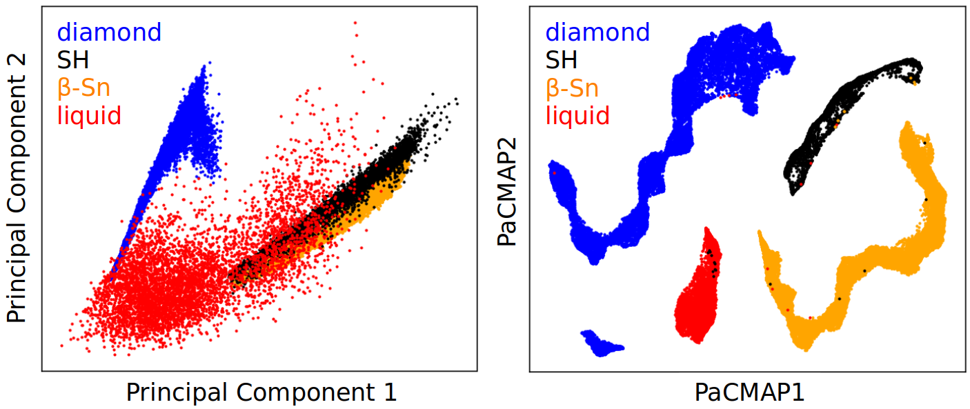
Figure 1: The clustering comparison of the PCA (left) and PaCMAP algorithm (right) of various silicon structures and phases.

The PaCMAP results on the identical dataset are presented in Fig. 1 (right). Not only are the $\beta$–Sn and SH phases distinctly differentiated, but also the discrimination between liquid and solid phases is achieved. The fractions of misclassified atoms for diamond, $\beta$–Sn, SH, and liquid phases are 0.00%, 0.04%, 0.33%, and 0.23%, respectively. The PaCMAP algorithm further divided the diamond structures into two clusters arising from a density jump.

3.1.2 Diamond point defects

In the subsequent analysis, we aim to localize interstitials and monovacancies in the diamond structure of silicon.

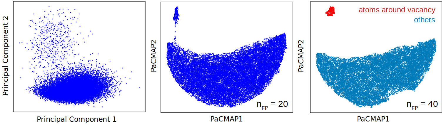
Figure 2: Left: The PCA clustering for monovacancies in the diamond silicon structure. Middle and right: The PaCMAP clustering for monovacancies in the diamond silicon structure varied in the number of further neighbors.

The monovacancy is not directly observable, but it can be detected by identifying the 4 nearest neighbors with which the missing atom would have formed a bond. PCA and PaCMAP clustering is depicted in Fig. 2. The clustering is more conclusive, when increasing the number of further neighbors $n_{FP}$ from the default 20 to 40. In 89% of the tested structures, PaCMAP identifies 4 atoms per structure, while in the remaining cases, it identifies 3, 5, or 6 atoms based on local distortions.

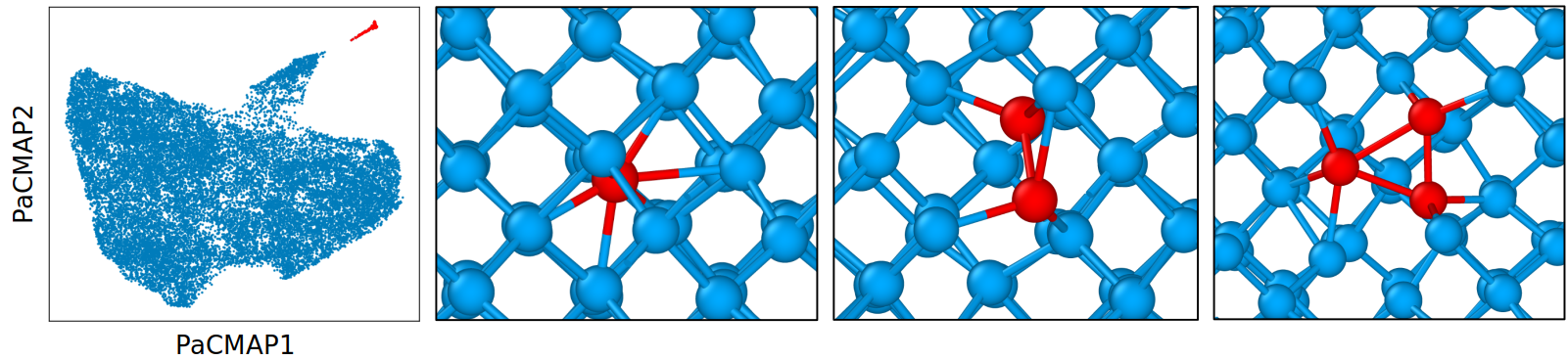
Figure 3: Left: The PaCMAP clustering for interstitials in the diamond silicon structure. The others: Three representative structures with atoms colored based on the cluster they belong to.

Identifying interstitial atoms is straightforward when their identity remains consistent throughout the simulation. However, if an interstitial atom undergoes a change in identity, additional post-analysis becomes necessary. The PaCMAP algorithm categorizes silicon atoms into three clusters (using $n_{FP}=40$), as illustrated in Fig. 3 (left). The largest cluster comprises atoms located far from the defect. In the middle cluster, we find atoms situated in close proximity to the interstitial. The smallest cluster in top right corner consists of atoms that are not arranged on a diamond lattice. Despite the presence of only one extra atom in each structure, the interstitial interacts strongly with its surroundings and can displace surrounding atoms from their lattice positions. In Fig. 3, we present three examples with varying degrees of local distortions.

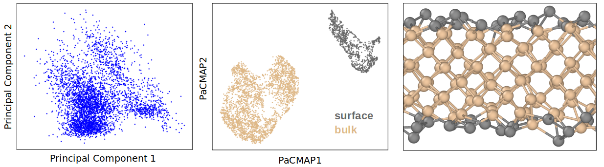
Figure 4: Left and middle: The clustering comparison of PCA and the PaCMAP algorithm for the diamond surface (001) of the silicon structure. Right: Atoms are colored based on the PaCMAP cluster they belong to.

3.1.3 Surface

Lastly, we focus on the diamond surfaces (001) of silicon. Despite the relatively small dataset (29 structures), PaCMAP identified two distinct clusters as shown in Fig. 4 (middle). Examining one of the structures depicted in Fig. 4 (right), it becomes apparent that the clusters correspond to bulk and surface atoms. Similar to previous cases, this differentiation arises purely from imperfect bonding or different local environments, and consequently, some atoms in the proximity of the surface may be classified as bulk if their bond count, distance, and bond angles with the bulk comply.

3.2 Water and ice

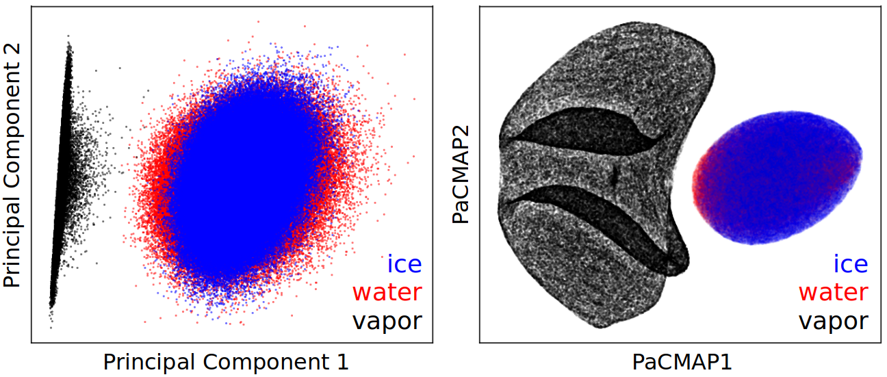
Figure 5: The clustering comparison of PCA (left) and the PaCMAP algorithm (right) for the ice, water, and vapor phases utilizing oxygen descriptors G_O(O-O,O-H).

Differentiation between liquid and ice phases poses a more challenging task than silicon. The mid to long-range ordering, a feature not primarily addressed by our potential descriptors, seems to be critical for the differentiation. While PaCMAP distinguishes vapor from the liquid and solid phases, the liquid and solid phases exhibit overlap using oxygen descriptors G_O(O-O,O-H) encompassing both oxygen-oxygen and oxygen-hydrogen interaction, as seen in Fig. 5. This stems from the greater significance attributed to the O-H bonds of water molecules compared to hydrogen bonds. Indeed, when the O-H bond length is fixed, as in the case of certain classical force fields, a complete separation between the liquid and solid phases occurs. Two options arise to address this: proposing new descriptors capable of achieving this distinction or applying a moving average to the existing ones. The moving average smoothens thermal fluctuations of O-H bonds, thereby revealing phase-related information. We observe the first cluster separation at 0.25 ps moving range interval. The increasing length of the moving average enhances the accuracy of phase differentiation, as shown in Fig. 6 (left) for G_O(O-O,O-H). For a moving average of 1 ps, misclassified water atoms amount to only 0.16%, and misclassified ice atoms are a mere 0.04%. The classification based on hydrogen descriptors G_H(H-H,H-O) yields 3 times higher misclassified error for water (0.46%), but only slightly worse results for ice (0.06%).

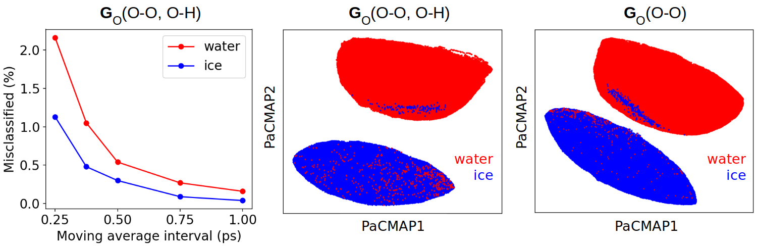
Figure 6: Left. The relationship between the misclassification percentage and the moving average interval (ps) for oxygen descriptors encompasses both oxygen-oxygen and oxygen-hydrogen interactions. Middle and Right: The variation in PaCMAP clustering when considering the presence (middle) or absence (right) of oxygen-hydrogen interactions within the oxygen descriptors. The descriptors of both approaches are averaged with a 1 ps moving interval.

Traditional methods based on bond orientational order parameters like Chill+ [28, 29] exclude hydrogen information. In our case, omitting the oxygen-hydrogen interaction G_O(O-O) triples classification error for ice (from 0.04 % to 0.12%), but reduces classification error from 0.16% to 0.09 % for water.

In the previous case, we compared the structures of bulk water and ice phases. A more challenging task is to identify an ice nucleus within the liquid phase, as their interface is also encompassed. The resulting PaCMAP clustering is not capable of distinctly differentiating between the phases even after applying the moving average, as shown in Fig. 7 (left). Although a cluster is visibly forming in the upper right, it is not sufficiently distinct. The given structure contains about 75,000 molecules in the liquid phase and about 2000 molecules in the solid phase resulting in an enormous class imbalance. Augmenting the dataset with an additional 1000 local environments of ice bulk enables complete cluster separation (Fig. 7 middle). However, only partial overlap with the ice bulk environment in the newly separated cluster is observed. The non-overlapping segment of the cluster corresponds to interface atoms. This is evident from the loss of periodicity at the edges of the visualized atoms belonging to the small cluster (Fig. 7 right).

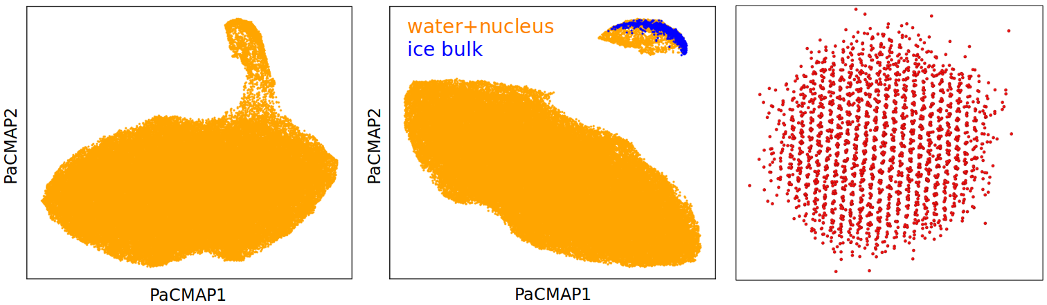
Figure 7: The PaCMAP algorithm clusters the water supercell with an ice nucleus (left), along with an additional 1000 ice bulk environments (middle). The identified ice nucleus is displayed on the right. A moving average of 0.75 ps is applied to the oxygen descriptors G_O(O-O,O-H).

3.3 Parametric clustering algorithm

Finally, we turn our attention to the most significant drawback of the PaCMAP algorithm, namely, its non-parametric nature. In other words, it is not possible to predict new datapoints after optimization. This limitation poses a significant constraint in real-world applications where the goal is to cluster training data and subsequently apply the learned mapping to new simulated datapoints. Although PaCMAP is a relatively fast algorithm [59], constantly applying it to large datasets would not be practical. A more practical approach involves utilizing PaCMAP to generate embedding/labels, which are then employed as output for supervised regression or classification tasks. Subsequently, a simple feedforward neural network can be easily trained and rapidly produce predictions for new local environments. To illustrate this approach, we trained a neural network with three hidden layers, each comprising 50 nodes and employing ReLU activation functions for bulk liquid and ice phases.

In Fig. 8, we compare the neural network’s predictions with the test reference dataset (PaCMAP mapping), proving visually that the neural network has successfully learned the underlying mapping of PaCMAP. However, for real-world applications, it would be more practical to utilize classification. The trained classification model trained on PaCMAP labels achieved a binary cross-entropy error of 0.0047 on the water test dataset and 0.0019 on the ice test dataset, indicating strong alignment between predicted probabilities and actual binary labels.

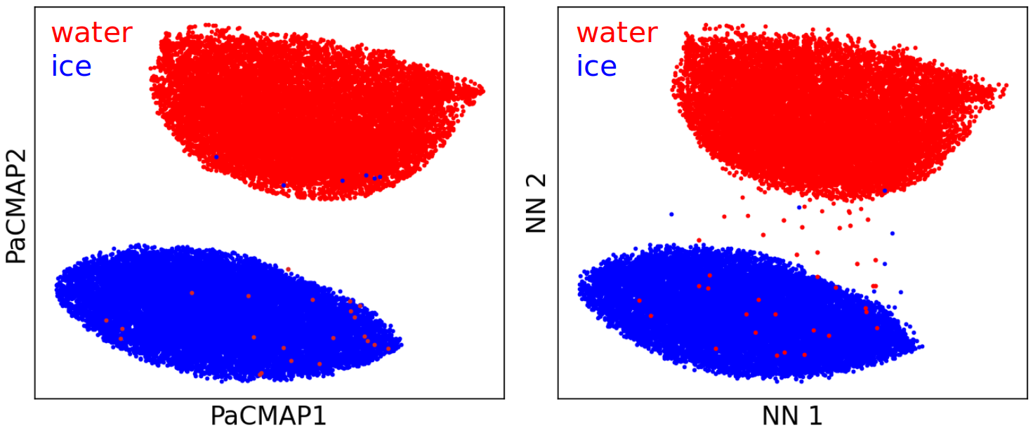
Figure 8: The comparison of reference test data (left) and predicted mapping by the neural network (right) to distinguish between water and ice. The test dataset size is 30,000 molecules.

We would like to note that the aforementioned scenario serves only for demonstration purposes. In practice, if we knew the labels from the beginning, the step with PaCMAP would be redundant, and it would be better to train the classification directly [31]. This approach is suitable for systems where atom labeling is difficult or there is no clear method of how to do it.

4 Conclusion

We have successfully demonstrated the applicability of atomistic potential descriptors for unsupervised identification of local atomic environments using silicon and water. The PaCMAP algorithm effectively distinguishes between different solid structures as well as between solid and liquid phases of silicon. Additionally, the algorithm can localize interstitial, monovacancy, and surface atoms in diamond structure, unlike the commonly used PCA method.

In the latter part, we have found that the use of oxygen descriptors including also oxygen-hydrogen interactions, proved to be the most effective for the classification of water and ice. Class imbalance in an ice nucleus surrounded by liquid can be addressed by incorporating additional ice bulk local atomic environments. PaCMAP is not only able to identify the crystalline phase but also interface atoms. It was also shown that PaCMAP mapping can be trained using a simple neural network, enabling the fast classification of new data points.

Although we have applied PaCMAP to systems that are amenable to traditional order parameter approaches, unsupervised algorithms are not intended to replace traditional approaches entirely. Their primary advantage lies in handling systems where order parameters are either unknown or computationally expensive to obtain.

References

References

- [1] Jörg Behler and Gábor Csányi. Machine learning potentials for extended systems: a perspective. The European Physical Journal B, 94:1–11, 2021.
- [2] Frank Noé, Simon Olsson, Jonas Köhler, and Hao Wu. Boltzmann generators: Sampling equilibrium states of many-body systems with deep learning. Science, 365(6457):eaaw1147, 2019.
- [3] Peter Wirnsberger, George Papamakarios, Borja Ibarz, Sébastien Racanière, Andrew J Ballard, Alexander Pritzel, and Charles Blundell. Normalizing flows for atomic solids. Machine Learning: Science and Technology, 3(2):025009, 2022.
- [4] Ziyue Zou, Eric R Beyerle, Sun-Ting Tsai, and Pratyush Tiwary. Driving and characterizing nucleation of urea and glycine polymorphs in water. Proceedings of the National Academy of Sciences, 120(7):e2216099120, 2023.
- [5] Hendrik Jung, Roberto Covino, A Arjun, Christian Leitold, Christoph Dellago, Peter G Bolhuis, and Gerhard Hummer. Machine-guided path sampling to discover mechanisms of molecular self-organization. Nature Computational Science, pages 1–12, 2023.
- [6] Claudio Zeni, Robert Pinsler, Daniel Zügner, Andrew Fowler, Matthew Horton, Xiang Fu, Sasha Shysheya, Jonathan Crabbé, Lixin Sun, Jake Smith, et al. Mattergen: a generative model for inorganic materials design. arXiv preprint arXiv:2312.03687, 2023.
- [7] Ghanshyam Pilania, Chenchen Wang, Xun Jiang, Sanguthevar Rajasekaran, and Ramamurthy Ramprasad. Accelerating materials property predictions using machine learning. Scientific reports, 3(1):2810, 2013.
- [8] Yeonghun Kang, Hyunsoo Park, Berend Smit, and Jihan Kim. A multi-modal pre-training transformer for universal transfer learning in metal–organic frameworks. Nature Machine Intelligence, 5(3):309–318, 2023.
- [9] Alexander Stukowski. Structure identification methods for atomistic simulations of crystalline materials. Modelling and Simulation in Materials Science and Engineering, 20(4):045021, 2012.
- [10] Duo Li, FengChao Wang, ZhenYu Yang, and YaPu Zhao. How to identify dislocations in molecular dynamics simulations? Science China Physics, Mechanics & Astronomy, 57:2177–2187, 2014.
- [11] Cynthia L Kelchner, SJ Plimpton, and JC Hamilton. Dislocation nucleation and defect structure during surface indentation. Physical review B, 58(17):11085, 1998.
- [12] J Dana Honeycutt and Hans C Andersen. Molecular dynamics study of melting and freezing of small lennard-jones clusters. Journal of Physical Chemistry, 91(19):4950–4963, 1987.
- [13] Helio Tsuzuki, Paulo S Branicio, and José P Rino. Structural characterization of deformed crystals by analysis of common atomic neighborhood. Computer physics communications, 177(6):518–523, 2007.
- [14] GJ Ackland and AP Jones. Applications of local crystal structure measures in experiment and simulation. Physical Review B, 73(5):054104, 2006.
- [15] Emanuel A Lazar, Jian Han, and David J Srolovitz. Topological framework for local structure analysis in condensed matter. Proceedings of the National Academy of Sciences, 112(43):E5769–E5776, 2015.
- [16] Jan Jenke, Aparna PA Subramanyam, Marc Densow, Thomas Hammerschmidt, David G Pettifor, and Ralf Drautz. Electronic structure based descriptor for characterizing local atomic environments. Physical Review B, 98(14):144102, 2018.
- [17] Paul J Steinhardt, David R Nelson, and Marco Ronchetti. Bond-orientational order in liquids and glasses. Physical Review B, 28(2):784, 1983.
- [18] Wolfgang Lechner and Christoph Dellago. Accurate determination of crystal structures based on averaged local bond order parameters. The Journal of chemical physics, 129(11), 2008.
- [19] Jeremy C Palmer, Fausto Martelli, Yang Liu, Roberto Car, Athanassios Z Panagiotopoulos, and Pablo G Debenedetti. Metastable liquid–liquid transition in a molecular model of water. Nature, 510(7505):385–388, 2014.
- [20] Eduardo Sanz, Chantal Valeriani, Emanuela Zaccarelli, Wilson CK Poon, Michael E Cates, and Peter N Pusey. Avalanches mediate crystallization in a hard-sphere glass. Proceedings of the National Academy of Sciences, 111(1):75–80, 2014.
- [21] Yao Yang, Jihan Zhou, Fan Zhu, Yakun Yuan, Dillan J Chang, Dennis S Kim, Minh Pham, Arjun Rana, Xuezeng Tian, Yonggang Yao, et al. Determining the three-dimensional atomic structure of an amorphous solid. Nature, 592(7852):60–64, 2021.
- [22] Jeroen S Van Duijneveldt and D Frenkel. Computer simulation study of free energy barriers in crystal nucleation. The Journal of chemical physics, 96(6):4655–4668, 1992.
- [23] Valentino Bianco, P Montero de Hijes, Cintia P Lamas, Eduardo Sanz, and Carlos Vega. Anomalous behavior in the nucleation of ice at negative pressures. Physical Review Letters, 126(1):015704, 2021.
- [24] Pablo M Piaggi, Jack Weis, Athanassios Z Panagiotopoulos, Pablo G Debenedetti, and Roberto Car. Homogeneous ice nucleation in an ab initio machine-learning model of water. Proceedings of the National Academy of Sciences, 119(33):e2207294119, 2022.
- [25] Wanyu Zhao and Tianshu Li. On the challenge of sampling multiple nucleation pathways: A case study of heterogeneous ice nucleation on fcc (211) surface. The Journal of Chemical Physics, 158(12), 2023.
- [26] Pablo Montero de Hijes, Salvatore Romano, Alexander Gorfer, and Christoph Dellago. The kinetics of the ice–water interface from ab initio machine learning simulations. The Journal of Chemical Physics, 158(20), 2023.
- [27] Leila Separdar, José Pedro Rino, and Edgar Dutra Zanotto. Crystal growth kinetics in bas semiconductor: Molecular dynamics simulation and theoretical calculations. Acta Materialia, page 119716, 2024.
- [28] Emily B Moore, Ezequiel De La Llave, Kai Welke, Damian A Scherlis, and Valeria Molinero. Freezing, melting and structure of ice in a hydrophilic nanopore. Physical Chemistry Chemical Physics, 12(16):4124–4134, 2010.
- [29] Andrew H Nguyen and Valeria Molinero. Identification of clathrate hydrates, hexagonal ice, cubic ice, and liquid water in simulations: The chill+ algorithm. The Journal of Physical Chemistry B, 119(29):9369–9376, 2015.
- [30] Andreas Zöttl and Holger Stark. Emergent behavior in active colloids. Journal of Physics: Condensed Matter, 28(25):253001, 2016.
- [31] Philipp Geiger and Christoph Dellago. Neural networks for local structure detection in polymorphic systems. The Journal of chemical physics, 139(16), 2013.
- [32] Maxwell Fulford, Matteo Salvalaglio, and Carla Molteni. Deepice: A deep neural network approach to identify ice and water molecules. Journal of Chemical Information and Modeling, 59(5):2141–2149, 2019.
- [33] Marjolein Dijkstra and Erik Luijten. From predictive modelling to machine learning and reverse engineering of colloidal self-assembly. Nature materials, 20(6):762–773, 2021.
- [34] Ryan S DeFever, Colin Targonski, Steven W Hall, Melissa C Smith, and Sapna Sarupria. A generalized deep learning approach for local structure identification in molecular simulations. Chemical science, 10(32):7503–7515, 2019.
- [35] Satoki Ishiai, Katsuhiro Endo, and Kenji Yasuoka. Graph neural networks classify molecular geometry and design novel order parameters of crystal and liquid. The Journal of Chemical Physics, 159(6), 2023.
- [36] Satoki Ishiai, Katsuhiro Endo, Paul E Brumby, Amadeu K Sum, and Kenji Yasuoka. Novel approach for designing order parameters of clathrate hydrate structures by graph neural network. The Journal of Chemical Physics, 160(6), 2024.
- [37] Jie Huang, Gang Huang, and Shiben Li. A machine learning model to classify dynamic processes in liquid water. ChemPhysChem, 23(1):e202100599, 2022.
- [38] Hideo Doi, Kazuaki Z Takahashi, Kenji Tagashira, Jun-ichi Fukuda, and Takeshi Aoyagi. Machine learning-aided analysis for complex local structure of liquid crystal polymers. Scientific reports, 9(1):16370, 2019.
- [39] Juan Carrasquilla and Roger G Melko. Machine learning phases of matter. Nature Physics, 13(5):431–434, 2017.
- [40] Michele Ceriotti. Unsupervised machine learning in atomistic simulations, between predictions and understanding. The Journal of chemical physics, 150(15), 2019.
- [41] Stephan Frickenhaus, Srinivasaraghavan Kannan, and Martin Zacharias. Efficient evaluation of sampling quality of molecular dynamics simulations by clustering of dihedral torsion angles and sammon mapping. Journal of computational chemistry, 30(3):479–492, 2009.
- [42] Miguel L Teodoro, George N Phillips Jr, and Lydia E Kavraki. Understanding protein flexibility through dimensionality reduction. Journal of Computational Biology, 10(3-4):617–634, 2003.
- [43] Hiromi Baba, Ryo Urano, Tetsuro Nagai, and Susumu Okazaki. Prediction of self-diffusion coefficients of chemically diverse pure liquids by all-atom molecular dynamics simulations. Journal of Computational Chemistry, 43(28):1892–1900, 2022.
- [44] Vojtěch Spiwok and Blanka Králová. Metadynamics in the conformational space nonlinearly dimensionally reduced by isomap. The Journal of Chemical Physics, 135(22), 2011.
- [45] Nikolaos G Sgourakis, Myrna Merced-Serrano, Christos Boutsidis, Petros Drineas, Zheming Du, Chunyu Wang, and Angel E Garcia. Atomic-level characterization of the ensemble of the a (1–42) monomer in water using unbiased molecular dynamics simulations and spectral algorithms. Journal of molecular biology, 405(2):570–583, 2011.
- [46] Aldo Glielmo, Brooke E Husic, Alex Rodriguez, Cecilia Clementi, Frank Noé, and Alessandro Laio. Unsupervised learning methods for molecular simulation data. Chemical Reviews, 121(16):9722–9758, 2021.
- [47] James Chapman, Nir Goldman, and Brandon C Wood. Efficient and universal characterization of atomic structures through a topological graph order parameter. npj Computational Materials, 8(1):37, 2022.
- [48] Wesley F Reinhart, Andrew W Long, Michael P Howard, Andrew L Ferguson, and Athanassios Z Panagiotopoulos. Machine learning for autonomous crystal structure identification. Soft Matter, 13(27):4733–4745, 2017.
- [49] Wesley F Reinhart and Athanassios Z Panagiotopoulos. Automated crystal characterization with a fast neighborhood graph analysis method. Soft matter, 14(29):6083–6089, 2018.
- [50] Matthew Spellings and Sharon C Glotzer. Machine learning for crystal identification and discovery. AIChE Journal, 64(6):2198–2206, 2018.
- [51] Emanuele Boattini, Marjolein Dijkstra, and Laura Filion. Unsupervised learning for local structure detection in colloidal systems. The Journal of chemical physics, 151(15), 2019.
- [52] Xuan Zhang, Yifeng Yao, Hongyi Li, Andre Python, and Kenji Mochizuki. Fast crystal growth of ice vii owing to the decoupling of translational and rotational ordering. Communications Physics, 6(1):164, 2023.
- [53] Matias Nunez. Exploring materials band structure space with unsupervised machine learning. Computational Materials Science, 158:117–123, 2019.
- [54] Wesley F Reinhart. Unsupervised learning of atomic environments from simple features. Computational Materials Science, 196:110511, 2021.
- [55] Martin Wattenberg, Fernanda Viégas, and Ian Johnson. How to use t-sne effectively. Distill, 2016.
- [56] Subhrajyoty Roy. Trustworthy Dimensionality Reduction. PhD thesis, 06 2021.
- [57] Etienne Becht, Leland McInnes, John Healy, Charles-Antoine Dutertre, Immanuel W H Kwok, Lai Guan Ng, Florent Ginhoux, and Evan W Newell. Dimensionality reduction for visualizing single-cell data using umap. Nature Biotechnology, 37(1):38–44, December 2018.
- [58] Yingfan Wang, Haiyang Huang, Cynthia Rudin, and Yaron Shaposhnik. Understanding how dimension reduction tools work: An empirical approach to deciphering t-sne, umap, trimap, and pacmap for data visualization. 2020.
- [59] Haiyang Huang, Yingfan Wang, Cynthia Rudin, and Edward P. Browne. Towards a comprehensive evaluation of dimension reduction methods for transcriptomic data visualization. Communications Biology, 5(1), July 2022.
- [60] P Montero de Hijes, J R Espinosa, C Vega, and C Dellago. Minimum in the pressure dependence of the interfacial free energy between ice ih and water. The Journal of Chemical Physics, 158(12), 2023.
- [61] Diederik P. Kingma and Jimmy Ba. Adam: A method for stochastic optimization, 2017.
- [62] Albert P. Bartók, James Kermode, Noam Bernstein, and Gábor Csányi. Machine learning a general-purpose interatomic potential for silicon. Physical Review X, 8(4), December 2018.
- [63] Andreas Singraber, Tobias Morawietz, Jörg Behler, and Christoph Dellago. Parallel multistream training of high-dimensional neural network potentials. Journal of Chemical Theory and Computation, 15(5):3075–3092, April 2019.
- [64] Aidan P Thompson, H Metin Aktulga, Richard Berger, Dan S Bolintineanu, W Michael Brown, Paul S Crozier, Pieter J in’t Veld, Axel Kohlmeyer, Stan G Moore, Trung Dac Nguyen, et al. Lammps-a flexible simulation tool for particle-based materials modeling at the atomic, meso, and continuum scales. Computer Physics Communications, 271:108171, 2022.
- [65] Tobias Morawietz, Andreas Singraber, Christoph Dellago, and Jörg Behler. How van der waals interactions determine the unique properties of water. Proceedings of the National Academy of Sciences, 113(30):8368–8373, July 2016.
- [66] Oliver Wohlfahrt, Christoph Dellago, and Marcello Sega. Ab initio structure and thermodynamics of the rpbe-d3 water/vapor interface by neural-network molecular dynamics. The Journal of Chemical Physics, 153(14), 2020.
- [67] Masakazu Matsumoto, Takuma Yagasaki, and Hideki Tanaka. Genice: hydrogen-disordered ice generator, 2018.
- [68] JLF Abascal, E Sanz, R García Fernández, and C Vega. A potential model for the study of ices and amorphous water: Tip4p/ice. The Journal of chemical physics, 122(23), 2005.
- [69] Mark James Abraham, Teemu Murtola, Roland Schulz, Szilárd Páll, Jeremy C Smith, Berk Hess, and Erik Lindahl. Gromacs: High performance molecular simulations through multi-level parallelism from laptops to supercomputers. SoftwareX, 1:19–25, 2015.
- [70] Jörg Behler and Michele Parrinello. Generalized neural-network representation of high-dimensional potential-energy surfaces. Physical Review Letters, 98(14), April 2007.
- [71] Martin P Bircher, Andreas Singraber, and Christoph Dellago. Improved description of atomic environments using low-cost polynomial functions with compact support. Machine Learning: Science and Technology, 2(3):035026, June 2021.
- [72] Michael Gastegger, Ludwig Schwiedrzik, Marius Bittermann, Florian Berzsenyi, and Philipp Marquetand. wacsf—weighted atom-centered symmetry functions as descriptors in machine learning potentials. The Journal of chemical physics, 148(24), 2018.
- [73] Alexander Stukowski. Visualization and analysis of atomistic simulation data with OVITO-the Open Visualization Tool. Modelling and Simulation in Materials Science and Engineering, 18(1), JAN 2010.
- [74] Adam Paszke, Sam Gross, Francisco Massa, Adam Lerer, James Bradbury, Gregory Chanan, Trevor Killeen, Zeming Lin, Natalia Gimelshein, Luca Antiga, Alban Desmaison, Andreas Kopf, Edward Yang, Zachary DeVito, Martin Raison, Alykhan Tejani, Sasank Chilamkurthy, Benoit Steiner, Lu Fang, Junjie Bai, and Soumith Chintala. Pytorch: An imperative style, high-performance deep learning library. In Advances in Neural Information Processing Systems 32, pages 8024–8035. Curran Associates, Inc., 2019.
- [75] G. A. Voronin, C. Pantea, T. W. Zerda, L. Wang, and Y. Zhao. In situx-ray diffraction study of silicon at pressures up to 15.5 gpa and temperatures up to 1073 k. Physical Review B, 68(2), July 2003.
- [76] Bartomeu Monserrat, Jan Gerit Brandenburg, Edgar A Engel, and Bingqing Cheng. Liquid water contains the building blocks of diverse ice phases. Nature communications, 11(1):5757, 2020.