Data Scoping: Effectively Learning the Evolution of Generic Transport PDEs

Abstract

Transport phenomena (e.g., fluid flows) are governed by time-dependent partial differential equations (PDEs) describing mass, momentum, and energy conservation, and are ubiquitous in many engineering applications. However, deep learning architectures are fundamentally incompatible with the simulation of these PDEs. This paper clearly articulates and then solves this incompatibility. The local-dependency of generic transport PDEs implies that it only involves local information to predict the physical properties at a location in the next time step. However, the deep learning architecture will inevitably increase the scope of information to make such predictions as the number of layers increases, which can cause sluggish convergence and compromise generalizability. This paper aims to solve this problem by proposing a distributed data scoping method with linear time complexity to strictly limit the scope of information to predict the local properties. The numerical experiments over multiple physics show that our data scoping method significantly accelerates training convergence and improves the generalizability of benchmark models on large-scale engineering simulations. Specifically, over the geometries not included in the training data for heat transferring simulation, it can increase the accuracy of Convolutional Neural Networks (CNNs) by 21.7 % and that of Fourier Neural Operators (FNOs) by 38.5 % on average.

Figure 1: The target problem. (a) The deep learning architecture inevitably expands the scope of input data used for the prediction at one position as the number of layers increases, which contradicts the local-dependency assumption for a generic transport system. (b) The data scoping method proposed in this paper can ensure that the scope of the input data stays constant regardless of the number of layers, which decouples the expressiveness and local dependency of neural networks.

1 Introduction

Generic transport equations, a set of time-dependent partial differential equations (PDEs), describe the evolutions of the extensive properties in a physical system, such as mass, momentum, and energy. Derived from the conservation laws governing these properties, these equations are fundamental to understanding various physical phenomena in science and engineering, such as mass diffusion equations, heat transfer equations, and Navier–Stokes equations. The high-fidelity and rapid simulations of complex physical systems based on generic transport equations play a critical role in addressing design and prediction challenges in diverse fields where the solutions of many instances of PDE in different coefficients, initial conditions (IC) and boundary conditions (BC) are required, including airplane design [21], metal additive manufacturing control [5], weather forecasting [25], drug delivery [3], and pandemic outbreak modeling [26]. Traditionally, solving these PDEs in discretized forms, such as finite difference methods, finite element methods, and finite volume methods, incurs a cubic relationship between domain resolution and computation cost [13], which means that a 10-fold increase in resolution leads to a thousandfold increase in the computational cost. This computational challenge becomes apparent when considering realistic problems. For instance, the chord length of an airplane is about 2 m while the smallest eddy scale is $O(10^{-6})$ m. The advancements in computation infrastructure, such as GPUs, TPUs, and the relevant parallel computing platform, have paved the way for the success of machine learning (ML). This, in turn, signals a paradigm shift in scientific computation, with ML techniques emerging as valuable tools for addressing the limitations posed by traditional numerical frameworks.

Contributions

This paper introduces a data scoping method to enhance the generalizability of data-driven models predicting time-dependent physics properties in generic transport problems by decoupling the expressiveness and local-dependency of the neural operator, as illustrated in Figure 1. Our major contributions can be summarized as follows.

• We define the local-dependency of generic transport PDEs in the form of a neural operator. From that, the incompatibility between the current deep learning architecture and the local-dependency of generic transport PDEs is demonstrated.

• We establish a data scoping method that solves the incompatibility mentioned above. It serves as both a preprocessing step and a postprocessing step. As a preprocessing step, it transforms the domain into information windows before the model makes predictions, and as a postprocessing step, it integrates these information windows. The linear time complexity of the method underscores its efficiency and scalability across different problem sizes.

• We apply our method to two prominent neural network types — CNN and FNO — operating on regular grids. Numerical experiments are done over the data generated from the mass diffusion, fluid mechanics, and heat transfer with various coefficients and geometries. Our results demonstrate a significant enhancement in the convergence rate and generalization capabilities of these models.

2 Background

Physics-informed neural networks

Physics-informed neural networks (PINNs) have demonstrated the ability to learn the smooth solutions of known nonlinear PDEs with little or no data by incorporating PDE residuals into the training loss [27]. This approach has proven particularly valuable in solving inverse problems, enabling the identification of unknown coefficients in governing equations [11]. However, it is important to note that a single PINN model is typically trained to learn one specific instance of a PDE with specific coefficients, IC and BC [14]. Consequently, retraining the PINN model for a new instance of PDEs is necessary, and the associated large training cost stands out as a major limitation of the PINN framework [10]. This limitation poses a challenge to the generalizability and efficiency of PINNs, hindering their ability to overcome computation bottlenecks posed by traditional numerical methods.

Data-driven models

Data-driven models, which learn general physical patterns solely from data, hold significant promise for overcoming computation bottlenecks in approximating the solutions to a family of PDEs with various coefficients, IC and BC. [39, 1, 17, 7, 31, 13, 34, 36]. Despite the abundance of these such models, they commonly share a deep learning architecture characterized by multiple layers of basic neural networks, including Convolutional Neural Networks (CNNs), Recurrent Neural Networks (RNNs), Graph Convolutional Neural Networks (GCNNs), and Fourier Neural Operators (FNOs). The expressiveness and nonlinearity of these models are realized through iterative forward computations across multiple layers. The design of the basic neural networks is specifically tailored for compatibility with matrix operations, efficiently accelerated in parallel on GPUs or TPUs. These ML models exhibit remarkable computational cost reductions, often on the order of three magnitudes, compared to traditional numerical methods, once they are well-trained [8]. However, the performance of data-driven is intricately tied to the quality of the data they are trained on. Notably, the training data for these models is predominantly sourced from traditional numerical methods or experimental observations, both of which can be prohibitively expensive to obtain [28]. This cost factor becomes particularly pronounced when aiming for a model capable of generalization to various PDE coefficients, IC, and BC for realistic problems. While there have been notable efforts to enhance the generalizability of data-driven models by tailoring model structures[32, 20, 33, 35], the deep learning architecture applied in these models hinders their generalizability because it is incompatible with the local-dependency of generic transport PDEs as elaborated below.

Local-dependency of generic transport systems

A data-driven model for generic transport PDEs can be formulated as a neural operator, mapping the current status of the system into the status at the next time step. The evolution of the system can be obtained through iterative updates of the status using this neural operator. In this paper, we assume that the operator only takes the current system status to make the prediction. Note that there is another line of methods that takes multiple previous system statuses [17, 22, 38]. While it can improve prediction accuracy, it requires more data and increases the training burden, which causes scalability problems for large-scale simulations.

In the context of generic transport systems, the speed of information propagation is limited. This implies that the physics properties at a position in the next time step depend on the current status of its neighbors, which is called local-dependency. The size of the neighborhood is determined by the characteristic information speed and the time step. The neighborhood is called the information window, or simply “window” in this paper. So, the neural operator should also be local dependent. If the input scope is larger than the information window, it would incur noises that distract the model from capturing the true physics pattern in the data. While CNN and GCNN have the property of local-dependency, the deep learning architecture weakens such property because the scope of the input data used to make the prediction at a position is enlarged as the layer number increases, as illustrated in Figure 1 (a) and will be further discussed in Section 3.3.

Domain decomposition methods

The concept of data scoping in this paper shares similarities with domain decomposition methods commonly used in traditional numerical approaches. Domain decomposition methods aim to alleviate the hardware demands of solving a large domain by partitioning it into smaller regions that can be solved in parallel with defined interface conditions [9, 30]. A series of machine learning models have incorporated the concept of domain decomposition [15, 16, 10]. These models decompose the domain into subdomains, each assigned a PINN model that is trained independently. Information exchange between subdomains is facilitated by adjusting the boundary term or incorporating interface conditions in the training loss. Although these methods enhance computation speed by solving subdomains in parallel, they share limitations inherent in PINNs—specifically, they are tailored to a particular instance of a PDE and involve a time-consuming training process. Our data scoping method also supports parallel computation while it is designed for data-driven models that approximate the solutions of a family of PDEs.

3 Local-dependent Neural Operator

PDEs can be viewed as nonlinear operators that map between Banach function spaces. We formulate the data-driven models as the nonlinear operators approximating a family of PDEs following the work of Li et. al.[17].

3.1 Solution Operator of Generic Transport PDEs

Formulation

The domain of a generic transport system in $d$-dimensional space is denoted as $D\subset\mathbb{R}^{d}$ which is a bounded open set. Let $d_{u}$ be the dimension of the physical properties transported in the system. Let $d_{a}$ be the dimension of the constant properties of a specific instance of PDEs, such as coefficients and boundary geometric features. Let $\mathcal{A}=\mathcal{A}(D;\mathbb{R}^{d_{a}})$ and $\mathcal{U}=\mathcal{U}(D;\mathbb{R}^{d_{u}})$ be Banach spaces of functions that take values in $\mathbb{R}^{d_{a}}$ and $\mathbb{R}^{d_{u}}$, respectively. The constant properties of the system are denoted as $a\in\mathcal{A}$. The status of the system at time $t$ is denoted as $u^{t}\in\mathcal{U}$. For the convenience of formulation, the time dimension is discretized uniformly. We have $t=0,1,2,...,T$ with fixed timestep $\Delta t$ and maximum $T$. The evolution of the system from $t$ to $t+1$ can then be represented by a nonlinear operator $G^{{\dagger}}:\mathcal{A}\times\mathcal{U}\rightarrow\mathcal{U}$ in the way that

$$u^{t+1}=G^{{\dagger}}(a,u^{t}).$$ (1)

Given $a$ and the initial status of the system $u^{0}$, $u^{t}$ can be calculated by $G^{{\dagger}}$ in an iterative way for all $t=0,1,2,...$. So, $G^{{\dagger}}$ can be viewed as the solution operator of a family of generic transport PDEs characterized by $\mathcal{A}$.

Learning framework

Given $a_{j}$, the solution of the instance of PDEs specified by $a_{j}$ is the list $[u^{0}_{j},u^{1}_{j},...,u^{T}_{j}]$ which is denoted as $U_{j}$. Suppose we have observations $\{a_{j},U_{j}\}_{j=1}^{N}$ where $a_{j}\thicksim\mu$ is an i.i.d. sequence from the probability measure $\mu$ supported on $\mathcal{A}$, and $U_{j}$ is the corresponding solution of the PDEs specified by $a_{j}$. Our goal is to approximate $G^{{\dagger}}$ by constructing a parametric non-linear operator, named neural operator, $G_{\theta}:\mathcal{A}\times\mathcal{U}\rightarrow\mathcal{U}$, where $\theta\in\Theta$ denotes the set of neural network parameters. With a cost function $C:\mathcal{U}\times\mathcal{U}\rightarrow\mathbb{R}$, the neural operator is trained by the following learning framework

$$\min_{\theta\in\Theta}\mathbb{E}_{a_{j}\sim\mu}[\mathbb{E}_{u^{t}_{j}\sim U_{j}}[C(G_{\theta}(a_{j},u^{t}_{j}),u^{t+1}_{j})]].$$ (2)

Dicretization

The functions $a_{j}$ and $u_{j}$ are discretized for the ease of computation in practice. According to the definition in [14], the neural operator is mesh-independent, which means that with the same $G_{\theta}$ can be used for different discretizations and $C(G_{\theta}(a_{j},u^{t}_{j}),u^{t+1}_{j})$ should not have significant changes over different discretizations. In this paper, we limit the discussion to the same discretization, so we relax the mesh-independent requirements. We generalized the definition of the neural operator to any data-driven models that can take $a_{j}$ and $u^{t}_{j}$, output $u^{t+1}_{j}$ over the fixed discretization.

3.2 Local-dependency

The physical information in a generic transport system travels at a limited speed.

Definition 1.

Let $\delta$ be the maximal length that the physical information can travel in $\Delta t$. So, the physical properties at a point $x\in D$ can only be influenced by its neighborhood $U(x,\delta)=\{y|y\in D,d(x,y)<\delta\}$ within $\Delta t$ timestep. Let $d(\cdot,\cdot)$ be the distance metric defined in $\mathbb{R}^{d}$. To predict $u^{t+1}(x)$, we do not need the whole system status $u^{t}$, but only the system status in $U(x,\delta)$ is sufficient. $U(x,\delta)$ is defined as the local-dependent region of the system at $x$.

We define the segment of $u^{t}$ over $U(x,\delta)$ as

$$u^{t}|_{U(x,\delta)}:=\left\{\begin{array}[]{rcl}u^{t}&\mbox{for}&x\in U(x,\delta)\\ 0&\mbox{for}&x\notin U(x,\delta)\\ \end{array}\right\}$$ (3)

So, we can define the local-dependent operator for the generic transport system in Definition 2.

Definition 2.

A nonlinear operator $G^{{\dagger}}:\mathcal{A}\times\mathcal{U}\rightarrow\mathcal{U}$ is said to have the local-dependency property and thus called a local-dependent operator if it updates the system as

$$u^{t+1}(x)=G^{{\dagger}}(a|_{U(x,\delta)},u^{t}|_{U(x,\delta)}),\forall x\in D.$$

3.3 Incompatibility between deep learning and local-dependency

Here we explain why the deep learning architecture of neural operators weakens the local-dependency. A neural operator consists of multiple layers where each layer is a linear operator followed by a non-linear activation. The universal approximation theorem states that such architecture can accurately approximate any nonlinear operator [6]. The deep learning architecture of the neural operator for generic transport problems is formulated in an iterative way that

$$v_{0}=P(a_{j},u^{t}_{j})$$ (4)

$$v_{i+1}=\sigma(K_{\phi}(v_{i}))$$

$$u^{t+1}_{j}=Q(v_{m}).$$

At the beginning, the input $a_{j}$ and $u^{t}_{j}$ is concatenated and projected to a higher dimension space $\mathbb{R}^{d_{v}}$ using a local linear transformation $P:\mathbb{R}^{d_{a}+d_{u}}\rightarrow\mathbb{R}^{d_{v}}$. Next, a series of iterative updates are applied, generating $v_{0}\mapsto v_{1}...\mapsto v_{m}$, where each vector takes value in $\mathbb{R}^{d_{v}}$. Finally, $v_{m}$ is projected back by a local linear transformation $Q:\mathbb{R}^{d_{v}}\rightarrow\mathbb{R}^{d_{u}}$. Let $\mathcal{V}=\mathcal{V}(D;\mathbb{R}^{d_{v}})$ be a Banach space of functions that take values in $\mathbb{R}^{d_{v}}$. The iterative update consists of a parameterized linear operator $K_{\phi}:\mathcal{V}\rightarrow\mathcal{V}$ followed by a non-linear activation function $\sigma:\mathbb{R}\rightarrow\mathbb{R}$.

Common linear operators include graph-based operators [18], low-rank operators [2], multipole graph-based operators [19], and Fourier operators [14]. It is possible to define a linear operator that only involves the local information around a point. For example,convolution is one of the common linear operators. We can define a local-dependent convolution over local-dependent region $U(x,\delta)$ as

$$K_{\phi}(v_{i})(x)=\int_{U(x,\delta)}k_{\phi}(x-y)v_{i}(y)dy,\forall x\in D,$$ (5)

where $k_{\phi}$ is a family of parameterized periodic functions. However, under a neural operator that consist of multiple layers of the local-dependent convolutions, the local-dependent region at $x$ is larger than $U(x,\delta)$. Specifically, the size of the expanded local-dependent region is positive proportional to the layer number, which is stated in Theorem 1 and proved in Appendix A.

Theorem 1.

Let $G_{\theta}:\mathcal{A}\times\mathcal{U}\rightarrow\mathcal{U}$ be a neural operator consisting of $k$ layers of local-dependent convolution defined in Equation 5 where the interval of the convolution is the $U(x,\delta)$. While the local-dependent region of each convolution layer is $U(x,\delta)$, the local-dependent region of the neural operator at $x$ is $U(x,k\delta)$.

So, we are in such a dilemma. Under the deep learning architecture, to increase the expressiveness of neural network to account for the nonlinearity of the generic transport PDEs, we need to increase the layer number. But increasing the layer number results in expanding the scope of the information used to make the prediction, which might violate the local-dependency of time-dependent generic transport PDEs as defined in Definition 2.

3.4 Data scoping

Instead of limiting the scope of the linear operator to one layer, our idea is to limit the scope of input data directly. The data scoping method decomposes the data so that each operator only works on the segmentation $u^{t}|_{U(x,\delta)}$ defined in Equation 3. So, now we have

$$v_{0}=P(a_{j},u^{t}_{j}|_{U(x,\delta)})$$ (6)

$$v_{i+1}|_{U(x,\delta)}=\sigma(K_{\phi}(v_{i}|_{U(x,\delta)}))$$

$$u^{t+1}_{j}|_{U(x,\delta)}=Q(v_{m}|_{U(x,\delta)})$$

Under this formulation, the calculation of $u^{t+1}_{j}(x)$ only involves the information in $U(x,\delta)$ no matter the scope of the linear operator $K_{\phi}$. To realize the segmentation $u^{t}|_{U(x,\delta)}$ efficiently, we developed a data scoping method to partition the data into windows with prescribed sizes and integrate the predictions over the individual windows into the whole domain.

Given a domain discretized by a grid, as illustrated in Figure 2 (a), to predict the physical properties in the next timestep at one position (colored in black), it is assumed that the local region colored in grey contains sufficient information. So, instead of inputting the whole domain into the ML model, we should only input the relevant local region (colored in grey) to make the prediction (colored in orange). Our domain decomposition algorithm partitions the domain evenly into smaller windows and has the ML model make the predictions at the centers of the windows. The details of the domain decomposition and its reverse, window patching, algorithms are illustrated in Figure 4 and explained in Section B.2. While one decomposition of the domain only generates the prediction at the center of the windows, as shown in Figure 2 (b), we need decompositions over an expanded domain as illustrated in Figure 3 and detailed in Section B.1 to make the complete prediction as indicated in Figure 2 (c). The prediction integration algorithm illustrated in Figure 5 and detailed in Section B.3 explains how to obtain the prediction over the complete domain.

Figure 2: The overview of the method. (a) To predict the physical property at the black position, its neighbors (colored in grey) contain sufficient information. The prediction is colored in orange. (b) One decomposition of the domain can be used to make the predictions over a part of the domain. (c) Multiple decompositions and prediction integration algorithms are needed to make the prediction over the whole domain.

Figure 3: The example of expanding the domain in two steps. (a) Given window size $(3,3)$, a 2D domain with size $(7,7)$ needs to be expanded to be multiple of the window size. (b) In the first step, the domain is expanded to $(9,9)$ by padding the zeros at the end of each dimension. (c) In the second step, the domain is expanded to $(10,10)$ to be compatible with the prediction integration algorithm by padding zeros at the beginning and the end of each dimension.

Figure 4: The illustration of the domain decomposition and window patching for one partition. (a). A data batch of global domain. In this example, the data in 2D space with $X^{0}$ denoting the batch dimension, $X^{1}$, and $X^{2}$ denoting the two domain dimensions. The batch size is set as 4 and the domain is set to be decomposed into $3\times 3$ blocks in this example. (b) The batch is split into three parts in $x^{2}$ dimension. (c) The parts are stacked in $X^{0}$ dimensions to make a new batch with 12 batch sizes and $1\times 3$ blocks. (d) The batch is split into three parts in $x^{1}$ dimension. (e) The parts are stacked in $x^{0}$ dimension. (f) The original data is decomposed into $3\times 3$ blocks which are stacked to make a new batch with 36 batch size. (g) The ML model predicts the physical properties at the centers of the windows. (h) In a reverse of the decomposition process (b) to (e), the data shape is recovered to the original shape with the predictions made at the centers of each window.

Figure 5: The illustration of the data integration algorithm. (a) A batch of 2D data is viewed from the top where $X^{1}$ and $X^{2}$ are the two domain dimensions and the batch size dimension $x^{0}$ is not shown in the top view. The domain represented by the grid is expanded by padding the zeros which is the blank space near its boundary. (b) Multiple partitions are made over the expanded domain. The predictions over the partitions are made independently and only the predictions in the centers of the blocks are preserved for the prediction integration, which is colored in orange. (c) The prediction over the whole domain is integrated.

4 Numerical Experiments

In this section, we evaluate the proposed data scoping method in 2D Burgers’ equations for fluid dynamics and 3D heat transfer equations. We also report additional results for the 2D mass transport equation, which can be found in Appendix. C.1. By implementing the FNO and CNNs models with and without our data scoping method, its effects are revealed. The data generation processes are generalized here and detailed in Appendix C. The FNO and CNN models each have 4 layers with 20 hidden dimensions. The Adam optimizer [12] is employed with a learning rate of $0.0001$. Normalized $L_{2}$ is used as training and testing loss and the $R^{2}$ score is applied for validation metric. For the 2D problems, various window sizes were examined and their influences on the ML model performance were studied. For the 3D problem, it was determined that a window size of $7$ provides the best performance. The code is publicly available on .

4.1 2D Burgers’ equation

The Burgers’ equation is also one of the most representative PDEs representing a convection-diffusion scheme. The solution of such an equation displays certain interesting physical phenomena including temporal wave propagation, shock wave formulation, and viscous-related energy dissipation. Approximating these complex dynamics is a challenging task for a machine learning model with no a priori information about the underlying physics, and therefore makes it a good testing case for validating model performance. Details of the physical equations and data generation methods are discussed in Appendix. C.2.

Examples of decomposed model prediction and reconstruction on Burgers’ equation are reported in Figure .6. The interesting finding is that while the solution of Burgers’ equation, compared with mass transport, contains much more complicated and localized physical dynamics, the data scoping method is still able to reconstruct smooth and continuous physical dynamics even though the dynamics inside each regional sub-domain greatly vary from each other.

Figure 6: Decomposed and reconstructed model prediction on solving the time sequential Burgers’ equation. All displayed physical properties are normalized and dimensionless.

4.2 Heat transfer in metal additive manufacturing

Thermal simulations for metal additive manufacturing (AM) are important in multiple stages of product development that involve AM processes, including part design, process planning, process monitoring, and process control [29, 23, 4, 5]. They are the typical examples where the traditional numerical methods are too time-consuming while the data-driven ML models are difficult to generalize to the situations not included in the training data. We test the capability of our data scoping method in improving the generalizability of the ML models for thermal simulations of the AM process. The type of generic transport PDEs in this problem is the heat transfer PDEs. The PDEs formulation and the data generated process are discussed in Appendix C.3 To study the geometric generalizability of the ML models, we collected the simulation data of 10 parts with various geometries. Figure 14 shows the 10 parts and snapshots of the thermal simulations. A 10-fold leave-one-outside cross-validation (LOOCV) is performed to evaluate the $R^{2}$ accuracy of the ML models over the geometry not included in the training data. At one round of LOOCV, the data from 9 parts are assembled as training and test data with a 9:1 ratio, and the data from the rest of one part is used for validation. Examples of the prediction results can be found in Figure 15.

5 Results and Discussion

To understand how the localized operator behaves under the data scoping, we perform a sequence of numerical experiments of different solution frequencies as stated in Section C.1. We examine the reconstructed $R^{2}$ accuracy of the solved solution field by FNO in correlation with the decomposed domain size and the character frequency of the solution field and report the result in Figure 7.

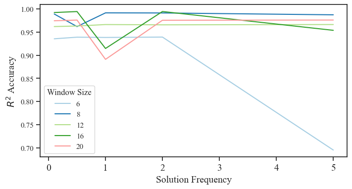
Figure 7: $R^{2}$ reconstruction accuracy of decomposed model predictions about window size and solution field frequency.

The frequency characterization of the domain reflects the speed of the information travels in the system. The higher the frequency, the faster the information travels and the larger the local-dependent region of the system becomes. For a fixed window size, as the frequency increase, the local-dependent region will gradually outgrows it and the model would be given less than required information to make the prediction at some point. That is why the accuracy drops dramatically as frequency increases for the smallest window size. It can also be explained in the view of frequency. A domain decomposition is a multiplication between the original solution function and a designated window function. Such multiplication therefore implements a frequency cutoff that adds high-frequency components to the Fourier domain of the original solution function. The higher the frequency of the original solution, the more divergence it will get when restricted to a localized area. To alleviate the effects of the frequency cut-off, we can increase the window size. However, as shown in Figure 7, a larger window size does not necessarily lead to better results. We see better solution quality as the decomposition window size increases from 6 to 10, however in high-frequency regions ($f>1$) as the window size gets larger than 12, the averaging accuracy obtained starts to decrease. It could be explained that the increased window size brings information not relevant to the local physical evolution, which is essentially noise so that it hinders the model from capturing the real physical pattern. It implies that there exists an optimal window size for a specific generic transport system. The results of the experiments indicate that the character frequency of the domain plays an important role in determining the window size.

The data scoping method can help accelerate the convergence of the ML models for generic transport problems by limiting the scope of input data. Figure 8 shows the average test loss over the 10-fold LOOCV of the CNNs and FNOs trained for the AM temperature prediction dataset with and without data scoping. The training processes with data scoping can reduce the test loss faster than the processes without data scoping. These results confirm our assumption that the coupling between the expressiveness and local dependency of deep learning architecture may expand the scope of input data beyond the travel range of the physics information, which can result in sluggish convergence. On the other hand, strictly limiting the scope of input data can speed up the training process.

The effects of the data scoping may differ depending on the type of ML models. As we can see in Figure 8, the FNOs gain a much larger improvement in the convergence rate than CNNs do. Such a difference might be originated from the local dependency of their linear operators. The linear operator of FNOs is the convolution in Fourier space, which involves the integral over the whole domain. So, the linear operator of FNOs is not local-dependent. Our data scoping method can make FNOs local-dependent while not influencing their powerful expressiveness in capturing the local physical patterns. On the other hand, the linear operator of CNNs is a kind of local convolution whose scope is prescribed by its kernel size. While the deep learning architecture can weaken its local dependency, CNNs are still more local-dependent than FNOs. Therefore, the improvements brought by the decoupling of the expressiveness and local dependency are more significant on FNOs than CNNs.

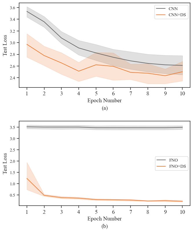
Figure 8: The average test loss with 95 % confidence intervals over the 10-fold LOOCV of the ML models trained for the AM temperature prediction dataset with and without data scoping. “DS” stands for data scoping. The stark difference between the effects of the data scoping method on CNN and FNO might be caused by the local dependency of their fundamental linear operator.

It should also be noted that the data scoping method can improve the generalizability of the ML models. Figure 9 shows the validation $R^{2}$ of the ML models over the 10-fold LOOCV of the AM temperature prediction dataset. The part index in the horizontal axis indicates the 10 parts with different geometries that are not included in the training and test of each validation round. So, the validation $R^{2}$ reveals the geometric generalizability of the models. As we can see, the data scoping method enhances the accuracy of all the validation data for both of the models. On average, CNNs are improved by 21.7 %, and FNOs are improved by 38.5%. This result supports our assumption that more data does not always beget better results. Especially, for the generic transport problems, the information outside of the local-dependent region is irrelevant to the local physical evolution. This extra information is essentially noises, which hinders the ML model from capturing the real physical patterns in the data. Therefore, limiting the scope of input data can effectively filter out the noises and help the ML models capture the real physical patterns contained in the data.

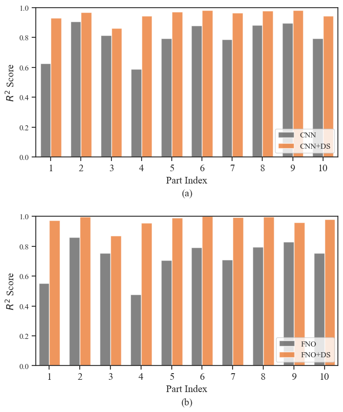
Figure 9: The data scoping method improves the geometric generalizability of the ML models for temperature prediction during AM processes. There are 10 rounds of leave-one-out cross-validation. In each round, the data of one geometric part is taken out and the ML models are trained on the data of the other 9 parts. Then, the ML models are validated over the data of the part not included in the training. “DS” stands for data scoping.

As analyzed in Section B.2, the time cost of the domain decomposition and window patching algorithms is linear with the largest block number in all dimensions $B_{max}$. A time cost experiment that collects the time cost of the two algorithms under different $B_{max}$ is conducted to demonstrate the linear time cost, as shown in Figure 10.

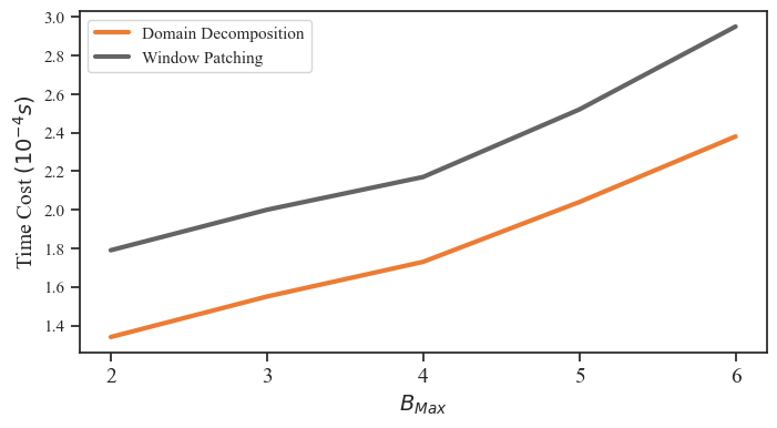
Figure 10: The time cost of the domain decomposition and window patching algorithm is linear with the largest block numbers in all dimensions $O(B_{max})$. For reference, the cost of FNO model inference is $2.1\times 10^{-3}$ s. The specification of the computer running the time analysis is AMD Ryzen Threadripper PRO 5955WX CPU with 16-Cores, an NVIDIA GeForce RTX 4090 GPU, and 258GiB of memory.

6 Conclusion and Future Direction

In this paper, we reveal the incompatibility between the deep learning architecture and the generic transport problems. We prove that the local-dependent region of deep learning models expands inevitably as the number of layers increases. On one hand, the expanded local-dependent region complicates the input data and introduces noise, which detrimentally impacts the convergence rate and generalizability of the models. On the other hand, the expressiveness of the ML models largely relies on the number of layers, so limiting the number of layers would weaken the performance of the models as well. Such a dilemma is caused by the coupled expressiveness and local-dependent property of deep learning architecture. To decouple the two, we propose an efficient data-scoping method. Through the numerical experiments over the data generated by three typical generic transport PDEs, we analyzed the properties of our data scoping method (e.g. the relationship among window size, system frequency, and error), and demonstrated its capabilities in accelerating convergence and enhancing generalizability of the ML models.

This approach has only been implemented on structured data now, but the idea has the potential for extension to unstructured data, like graphs. Since each partition is independent, parallel computation could accelerate the prediction integration significantly. By doing so, the scalability of our method, by computing each partition and each window independently, can be exploited and could have the potential for complex, large-scale generic transport problems.

Impact Statements

This paper presents work that seeks to broaden the application of machine learning methods in real-world engineering scenarios by improving the efficiency and robustness of neural network models for predicting physical properties. The authors do like to stress that, misusing the proposed method in safety-critical engineering simulations without sufficient validation can cause unexpected damage and negative social impact.

Appendix A Proofs

We prove Theorem 1 here.

Lemma 1.

Given a point $x$ in a metric space $M$ and positive real numbers $\delta_{1}$ and $\delta_{2}$, we have $\bigcup_{y\in U(x,\delta_{1})}U(y,\delta_{2})=U(x,\delta_{1}+\delta_{2})$.

Proof.

(1) $\forall z\in\bigcup_{y\in U(x,\delta_{1})}U(y,\delta_{2})$, $\exists y_{0}\in U(x,\delta_{1})$, s.t. $z\in U(y_{0},\delta_{2})$. According to triangle inequality, we have

$$d(z,x)\leq d(z,y_{0})+d(y_{0},x).$$ (7)

Since $d(z,y_{0})<\delta_{2}$ and $d(y_{0},x)<\delta_{1}$, we have

$$d(z,x)<\delta_{1}+\delta_{2}.$$ (8)

So, $z\in U(x,\delta_{1}+\delta_{2})$.

(2) $\forall z\in U(x,\delta_{1}+\delta_{2})$, if we assume $\nexists y\in U(x,\delta_{1})$ s.t. $z\in U(y,\delta_{2})$, we show in the following that it will result in contradiction. According to the assumption, we have $d(z,y)>\delta_{2},\forall y\in U(x,\delta_{1})$. We denote $\xi=\sup_{z\in U(x,\delta_{1}+\delta_{2})}d(z,x)$. Since $d(z,x)\leq d(z,y)+d(y,z)$, we have

$$\xi=\sup d(z,y)+\sup d(y,x).$$ (9)

Since $\sup d(y,x)=\delta_{1}$ and $\sup d(z,y)>\delta_{2}$, we have

$$\xi>\delta_{1}+\delta_{2},$$ (10)

which contradicts with $z\in U(x,\delta_{1}+\delta_{2})$. Therefore, $\exists y\in U(x,\delta_{1})$ s.t. $z\in U(y,\delta_{2})$. So, $z\in\bigcup_{y\in U(x,\delta_{1})}U(y,\delta_{2})$.

According to (1) and (2), we have $\bigcup_{y\in U(x,\delta_{1})}U(y,\delta_{2})=U(x,\delta_{1}+\delta_{2})$. ∎

Now we can prove Theorem 1.

Proof.

Since the non-linear activation function $\sigma$, and the linear project mapping $P$ and $Q$ do not influence the size of local-dependent region, we can simplify the expression of a neural operator as

$$v_{i+1}=K_{\phi}(v_{i}),$$ (11)

$$K_{\phi}(v_{i})(x)=\int_{U(x,\delta)}k_{\phi}(x-y)v_{i}(y)dy.$$

(1) When $k=1$, there is only one layer of local-dependent convolution whose integral is defined over $U(x,\delta)$. So the local-dependent region of $v_{1}(x)$ is $U(x,\delta)$.

(2) When $k=i$, we assume the local-dependent region of $v_{i}(x)$ is $U(x,i\delta)$. When $k=i+1$, we have

$$v_{i+1}(x)=\int_{U(x,\delta)}k_{\phi}(x-y)v_{i}(y)dy.$$ (12)

From Equation 12, we know that the calculation of $v_{i+1}(x)$ involves $v_{i}(y),\forall y\in U(x,\delta)$. So we have the local-dependent region of $v_{i+1}(x)$ as $\bigcup_{y\in U(x,\delta)}U(x,i\delta)=U(x,(i+1)\delta)$ according to Lemma 1. ∎

Appendix B Formulation of Data Scoping Method

B.1 Domain expansion

A grid $d-$dimension domain with size $(N_{1},...,N_{d})$ where $N_{i}\in\mathbb{N}^{+}$ is denoted as $D(N_{1},...,N_{d})$ or $D$ if the dimensions are given in the context. To decompose the domain into the windows with size $(W_{1},...,W_{d})$ where $W_{i}\in\mathbb{N}^{+}$ and make it compatible with the data integration algorithm, the domain needs to be expanded by two steps. The first step is to pad the zeros after the end of each dimension to make the dimension number as the multiple of $W_{i}$. The second step is to pad $[w/2]$ zeros at the beginning and $[(w-1)/2]$ zeros after the end of each dimension. Figure 3 illustrates the domain-expanding process in a 2D example. After the expansion, the new dimension number $N_{i}^{new}$ becomes

$$N_{i}^{new}=([(N_{i}-1)/W_{i}]+1)W_{i}+(W_{i}-1),\text{for }i=1,...,d,$$ (13)

where $[\cdot]$ is the operation that only keeps the integer part of a real number. In the following, the grid domain is always considered as the domain after expansion. The number of the windows of the decomposition in each dimension is denoted as $B_{i}$, referring as the block number, can be calculated as

$$B_{i}=[N_{i}/W_{i}].$$ (14)

B.2 Domain decomposition

Input data for the ML model is formed as batches. A batch of structured data can be represented as a tensor with size $(N_{b},N_{1},..,N_{d},N_{c})$ where $N_{b}$ is the batch number and $N_{c}$ is the channel dimension which is determined by the dimension of physical properties at a position. Given the window size $(W_{1},...,W_{d})$, our method aims to decompose the whole batch of data into a new tensor with size $(N_{b}*B_{i}*...*B_{d},W_{1},...,W_{d},N_{c})$. Appendix 1 shows the algorithm. Figure 4 illustrates a 2D example. In this example, we are given a batch of 2D data with size $(4,9,9,1)$ and the window size is $(3,3)$. The block number is $(3,3)$. After a sequence of splitting and stacking operations, the batch of the whole domain data is converted to a batch of the windows in the shape of $(36,3,3,1)$. For 2D data, there is twice splitting and twice stacking, while for 3D data, there is thrice splitting and thrice stacking. The time complexity of the splitting and stacking of the array data is $O(B_{max})$ where $B_{max}$ is the maximal among $B_{i},i=1,...,d$. The batch of the windows is then input into an ML model and the physical properties at the center of the windows are predicted as shown in Figure 4 (g). Then the window patching algorithm detailed in Appendix 2, a reverse of the decomposition operation, is followed to recover the batch of the whole domain from the batch of the windows. The window patching algorithm consists of the same number of splitting and stacking operations as the decomposition algorithm does, whose time complexity is also $O(B_{max})$. So the time complexity of the total algorithm is $O(B_{max})$.

B.3 Prediction integration

As shown in Figure 4 (h) the prediction over one decomposition can only give us the physical properties at the centers of the windows, to get the complete prediction over the whole domain, we need multiple decompositions which ensures that all the positions are the centers of some windows. Appendix 3 details the prediction integration algorithm. Figure 5 illustrates the prediction integration algorithm with a 2D example. Figure 5 (a) shows the 2D grid domain. The blank zone near the boundary indicates the padding zeros. The original domain size is $(9,9)$ and the expanded domain size is $(11,11)$. With $(3,3)$ window size, the block number for one decomposition is $(3,3)$. As each decomposition can be used to predict the center of all its windows, we need $3\times 3$ different decompositions of the domain which can cover all the positions as shown in Figure 5 (b) and (c). In general case, it is required to have $\prod_{i=1}^{d}W_{i}$ decompositions to cover the whole domain. The window size $W_{i}$ is a small number compared with the domain dimension. Since the predictions over the different decompositions are independent, they can be calculated in parallel. Therefore, the time complexity of the prediction integration algorithm is the constant multiple of the time complexity of the ML model inference.

Algorithm 1 Domain decomposition

1:procedure Chunk-domain($x,B,d$) $\triangleright$ domain tensor, block numbers, dimension number

2:     $i\leftarrow 0$

3:     while $i\neq d$ do

4:         $x\leftarrow Split(x,B_{i},i+1)$ $\triangleright$ Split the x along $(i+1)$-th dimension into $B_{i}$ blocks.

5:         $x\leftarrow Stack(x,0)$ $\triangleright$ Stack the blocks along $0$-th dimension.

6:         $i\leftarrow i+1$      

Algorithm 2 Window patching

1:procedure Window-patching($x,b,B,d$) $\triangleright$ domain tensor, batch size, block numbers, dimension number

2:     $i\leftarrow 0$

3:     while $i\not=d$ do

4:         if $d-i-2<0$ then

5:              $V\leftarrow b$

6:         else

7:              $V\leftarrow b\times\prod_{j=0}^{d-i-2}B_{i}$          

8:         $x\leftarrow Split(x,V,0)$ $\triangleright$ Split the x along $0$-th dimension into $V$ blocks.

9:         $x\leftarrow Stack(x,d-i)$ $\triangleright$ Stack the blocks along $(d-i)$-th dimension.

10:         $i\leftarrow i+1$      

Algorithm 3 Prediction integration

1:procedure Prediction-integration($x,NN,w,b,B,N,P,d$) $\triangleright$ domain tensor, neural network, window size, batch size, block number, domain size, window points, dimension number

2:     $x\leftarrow\text{Expand-Domain}(x,w,N)$ $\triangleright$ Expand the domain by padding zeros

3:     for $p\in P$ do $\triangleright$ Loop over all the points in a window

4:         $x_{p}\leftarrow x[p:p+wB]$. $\triangleright$ Select the part of $x$ that starts from $p$ with size $wB$

5:         $x_{p}\leftarrow\text{Chunk-Domain}(x_{p},B,d)$ $\triangleright$ Decompose the data

6:         $y_{p}\leftarrow NN(x_{p})$ $\triangleright$ Make the prediction over the decomposed data

7:         $y_{p}\leftarrow\text{Window-Patch}(y_{p},b,B,d)$ $\triangleright$ Recover the domain to the original shape

8:         $\{y\}\leftarrow y_{p}[w/2]$ $\triangleright$ Store the values at the window centers of $y_{p}$      

Appendix C Data generation

C.1 Mass transport equation

The transport of mass can be seen as one of the most fundamental PDEs with variation in both time and space. It also enjoys the benefit of having a fully closed mathematical solution, and that the problem can be carefully constructed to show the solution field of different character frequencies. We test the data scoping method’s representation ability on solution functions of different frequencies to understand the decomposition method’s performance on questions including how small the decomposition can get, and how wide the frequency range the decomposition can capture before the model starts to lose accuracy due to domain cut-offs in Section. 5.

A typical mass transport equation can be expressed as Equation 15:

$$\frac{\partial u}{\partial t}=-c\cdot\nabla\mathbf{u},$$ (15)

and the exact mathematical equation can be written as Equation

$$\mathbf{u(t)}=\mathbf{u}_{0}(x-ct),$$ (16)

for any initial condition $\mathbf{u}_{0}$, transport speed $c$ and given temporal stamp $t$. We can thus construct the frequency of our solution by determining the frequency of the initial condition. Variants of the solution frequency are shown in Figure. 11

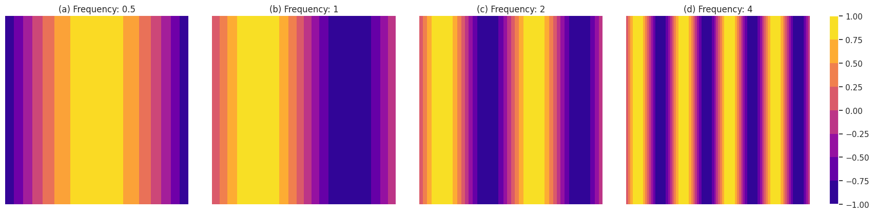
Figure 11: Solution of the mass transport equation of a $\sin$ wave in different frequencies. All displayed physical properties are normalized and dimensionless. (a) $f=0.5$; (b) $f=1.0$, (c) $f=2.0$, (d) $f=4.0$

Examples of decomposed model prediction and reconstructions on mass transport equations using a solution frequency of 5 and window size of 10 are reported in Figure .12. We see that The model can achieve very high correspondence with physical dynamics even when trained on small windows that reduced the original data size by more than 36 times (6 times on each dimension). The reconstruction method applied in Figure. 5 also helped to smooth out the entire solution field, suggesting the potential of the model application in reconstructing physical dynamics at minimum cost.

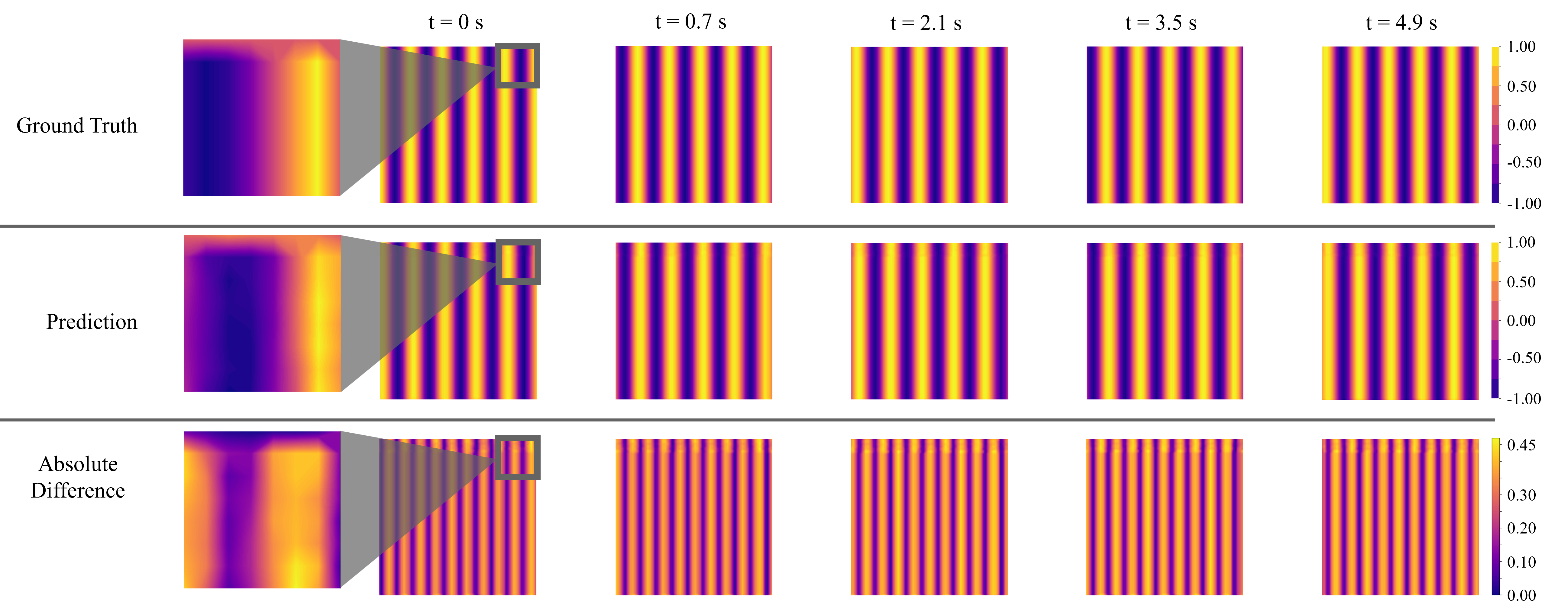
Figure 12: Decomposed and reconstructed model prediction on solving the time sequential mass transport equation. All displayed physical properties are normalized and dimensionless.

C.2 Burgers’ equation

In our experiment, we implement the viscous version of Burgers’ equation as described by Eq. 17:

$$\frac{\partial\mathbf{u}}{\partial t}+(\mathbf{u}\cdot\nabla)\mathbf{u}=\nu\nabla^{2}\mathbf{u},~{}\mathbf{x}\in D$$ (17)

where $\mathbf{u}$ denotes the velocity of the fluid, $\mathbf{x}$ and $t$ are spatial and temporal coordinates respectively, and $\nu$ is the viscosity of the fluid.

We solve Eq. 17 with $\nu=0.01Pa\cdot s$, and a time step of $0.1s$ for a total of 10 seconds with randomly initialized velocity Gaussian distribution as the initial condition. The simulations of the Burgers’ equation under different initial conditions are performed in FEniCS on a 2D mesh of $80\times 80$ elements per unit. Four Burgers’ equation solutions computed in four different initial velocity distributions are shown in Fig. 13.

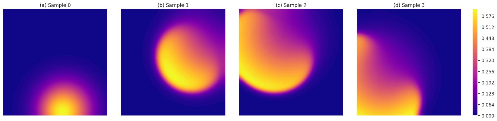
Figure 13: Solution of the Burgers’ equation in 2D with random initialization. All displayed physical properties are normalized and dimensionless.

C.3 AM temperature data

Let $\Omega$ denote a domain, and $\partial\Omega$ its boundary. $\partial\Omega_{\mathrm{H}}$ represents the part at which heat is transferred to the surroundings with constant temperature $T_{\infty}$, and $\partial\Omega_{\mathrm{D}}$ the part at which the temperature is fixed at $T_{\mathrm{D}}$. The temperature evolution within $\Omega$ is governed by the heat transfer PDEs:

$$\rho c_{p}\dot{T} =\nabla\cdot(k_{p}\nabla T), \forall\mathbf{x}\in\partial\Omega$$ (18)

$$-\mathbf{n}\cdot k_{p}\nabla T =h_{\mathrm{c}}(T-T_{\infty}), \forall\mathbf{x}\in\partial\Omega_{\mathrm{H}}$$

$$T =T_{\mathrm{D}}, \forall\mathbf{x}\in\partial\Omega_{\mathrm{D}}.$$

Here, $\rho$, $c_{\mathrm{p}}$, and $k_{\mathrm{p}}$ are the temperature-dependent density, specific heat capacity, and conductivity of the material, respectively. The vector $\mathbf{n}$ is the unit outward normal of the boundary at coordinate $\mathbf{x}$.

We utilized the thermal simulation algorithm developed in [24] to solve the partial differential equations described in Equation 18 for the wired-based DED process. This algorithm uses the discontinuous DGFEM to spatially discretize the problem and the explicit forward Euler time-stepping scheme to advance the solution in time. The algorithm activates elements based on the predefined toolpath. Newly deposited elements are initialized at elevated temperatures, after which they are allowed to cool according to Equation 18. The temperature of the substrate’s bottom face is kept fixed at $T_{\infty}=25^{\circ}C$. On all other faces, convection, and radiation to the surrounding air at $T_{\infty}$ is modeled. We set the tool moving speed to $5mm/s$. All geometric models were discretized with a resolution of $20\times 20\times 20$, with an element size of $2mm$. Our simulations utilized S355 structural steel as the material, with material properties as given in [24].

We run the AM thermal simulation over 10 parts with different geometries as shown in Figure 14. The 10 geometries are randomly generated by SkexGen [37], which contains various common mechanical features, such as holes, ribs, and pillars. Figure 15 shows the examples of the temperature prediction made by FNO with data scoping over the samples randomly selected from the validation data of part 1.

Figure 14: AM temperature prediction dataset. (a) The 10 parts with various geometries. (b) The temperature histories of the AM process that building the 10 parts are generated.

Figure 15: AM temperature prediction made by FNOs with data scoping. The samples are randomly selected from the validation data of part 1.

References

- Belbute-Peres et al. [2020] Belbute-Peres, F. D. A., Economon, T., and Kolter, Z. Combining differentiable pde solvers and graph neural networks for fluid flow prediction. In international conference on machine learning, pp. 2402–2411. PMLR, 2020.
- Börm & Grasedyck [2004] Börm, S. and Grasedyck, L. Low-rank approximation of integral operators by interpolation. Computing, 72:325–332, 2004.
- Boso et al. [2020] Boso, D. P., Di Mascolo, D., Santagiuliana, R., Decuzzi, P., and Schrefler, B. A. Drug delivery: Experiments, mathematical modelling and machine learning. Computers in biology and medicine, 123:103820, 2020.
- Chen et al. [2023] Chen, J., Xu, W., Baldwin, M., Nijhuis, B., Boogaard, T. v. d., Gutiérrez, N. G., Narra, S. P., and McComb, C. Capturing local temperature evolution during additive manufacturing through fourier neural operators. In International Design Engineering Technical Conferences and Computers and Information in Engineering Conference, volume 87295, pp. V002T02A085. American Society of Mechanical Engineers, 2023.
- Chen et al. [2024] Chen, J., Pierce, J., Williams, G., Simpson, T. W., Meisel, N., Prabha Narra, S., and McComb, C. Accelerating thermal simulations in additive manufacturing by training physics-informed neural networks with randomly-synthesized data. Journal of Computing and Information Science in Engineering, pp. 1–14, 2024.
- Chen & Chen [1995] Chen, T. and Chen, H. Universal approximation to nonlinear operators by neural networks with arbitrary activation functions and its application to dynamical systems. IEEE Transactions on Neural Networks, 6(4):911–917, 1995.
- Esmaeilzadeh et al. [2020] Esmaeilzadeh, S., Azizzadenesheli, K., Kashinath, K., Mustafa, M., Tchelepi, H. A., Marcus, P., Prabhat, M., Anandkumar, A., et al. Meshfreeflownet: A physics-constrained deep continuous space-time super-resolution framework. In SC20: International Conference for High Performance Computing, Networking, Storage and Analysis, pp. 1–15. IEEE, 2020.
- Ganti & Khare [2020] Ganti, H. and Khare, P. Data-driven surrogate modeling of multiphase flows using machine learning techniques. Computers & Fluids, 211:104626, 2020.
- Haddadi et al. [2017] Haddadi, B., Jordan, C., and Harasek, M. Cost efficient cfd simulations: Proper selection of domain partitioning strategies. Computer Physics Communications, 219:121–134, 2017.
- Jagtap & Karniadakis [2021] Jagtap, A. D. and Karniadakis, G. E. Extended physics-informed neural networks (xpinns): A generalized space-time domain decomposition based deep learning framework for nonlinear partial differential equations. In AAAI spring symposium: MLPS, volume 10, 2021.
- Jagtap et al. [2020] Jagtap, A. D., Kharazmi, E., and Karniadakis, G. E. Conservative physics-informed neural networks on discrete domains for conservation laws: Applications to forward and inverse problems. Computer Methods in Applied Mechanics and Engineering, 365:113028, 2020.
- Kingma & Ba [2014] Kingma, D. P. and Ba, J. Adam: A method for stochastic optimization. arXiv preprint arXiv:1412.6980, 2014.
- Kochkov et al. [2021] Kochkov, D., Smith, J. A., Alieva, A., Wang, Q., Brenner, M. P., and Hoyer, S. Machine learning–accelerated computational fluid dynamics. Proceedings of the National Academy of Sciences, 118(21):e2101784118, 2021.
- Kovachki et al. [2021] Kovachki, N., Li, Z., Liu, B., Azizzadenesheli, K., Bhattacharya, K., Stuart, A., and Anandkumar, A. Neural operator: Learning maps between function spaces. arXiv preprint arXiv:2108.08481, 2021.
- Li et al. [2019] Li, K., Tang, K., Wu, T., and Liao, Q. D3m: A deep domain decomposition method for partial differential equations. IEEE Access, 8:5283–5294, 2019.
- Li et al. [2020a] Li, W., Xiang, X., and Xu, Y. Deep domain decomposition method: Elliptic problems. In Mathematical and Scientific Machine Learning, pp. 269–286. PMLR, 2020a.
- Li et al. [2020b] Li, Z., Kovachki, N., Azizzadenesheli, K., Liu, B., Bhattacharya, K., Stuart, A., and Anandkumar, A. Fourier neural operator for parametric partial differential equations. arXiv preprint arXiv:2010.08895, 2020b.
- Li et al. [2020c] Li, Z., Kovachki, N., Azizzadenesheli, K., Liu, B., Bhattacharya, K., Stuart, A., and Anandkumar, A. Neural operator: Graph kernel network for partial differential equations. arXiv preprint arXiv:2003.03485, 2020c.
- Li et al. [2020d] Li, Z., Kovachki, N., Azizzadenesheli, K., Liu, B., Stuart, A., Bhattacharya, K., and Anandkumar, A. Multipole graph neural operator for parametric partial differential equations. Advances in Neural Information Processing Systems, 33:6755–6766, 2020d.
- Li et al. [2023] Li, Z., Kovachki, N. B., Choy, C., Li, B., Kossaifi, J., Otta, S. P., Nabian, M. A., Stadler, M., Hundt, C., Azizzadenesheli, K., et al. Geometry-informed neural operator for large-scale 3d pdes. arXiv preprint arXiv:2309.00583, 2023.
- Martins [2022] Martins, J. R. Aerodynamic design optimization: Challenges and perspectives. Computers & Fluids, 239:105391, 2022.
- Mozaffar et al. [2021] Mozaffar, M., Liao, S., Lin, H., Ehmann, K., and Cao, J. Geometry-agnostic data-driven thermal modeling of additive manufacturing processes using graph neural networks. Additive Manufacturing, 48:102449, 2021.
- Mozaffar et al. [2023] Mozaffar, M., Liao, S., Jeong, J., Xue, T., and Cao, J. Differentiable simulation for material thermal response design in additive manufacturing processes. Additive Manufacturing, 61:103337, 2023.
- Nijhuis et al. [2021] Nijhuis, B., Geijselaers, B., and van den Boogaard, T. Efficient thermal simulation of large-scale metal additive manufacturing using hot element addition. Computers & Structures, 245:106463, 2021.
- Pathak et al. [2022] Pathak, J., Subramanian, S., Harrington, P., Raja, S., Chattopadhyay, A., Mardani, M., Kurth, T., Hall, D., Li, Z., Azizzadenesheli, K., et al. Fourcastnet: A global data-driven high-resolution weather model using adaptive fourier neural operators. arXiv preprint arXiv:2202.11214, 2022.
- Raheja et al. [2023] Raheja, S., Kasturia, S., Cheng, X., and Kumar, M. Machine learning-based diffusion model for prediction of coronavirus-19 outbreak. Neural Computing and Applications, 35(19):13755–13774, 2023.
- Raissi et al. [2019] Raissi, M., Perdikaris, P., and Karniadakis, G. E. Physics-informed neural networks: A deep learning framework for solving forward and inverse problems involving nonlinear partial differential equations. Journal of Computational physics, 378:686–707, 2019.
- Sun et al. [2020] Sun, L., Gao, H., Pan, S., and Wang, J.-X. Surrogate modeling for fluid flows based on physics-constrained deep learning without simulation data. Computer Methods in Applied Mechanics and Engineering, 361:112732, 2020.
- Sun et al. [2022] Sun, Z., Ma, Y., Ponge, D., Zaefferer, S., Jägle, E. A., Gault, B., Rollett, A. D., and Raabe, D. Thermodynamics-guided alloy and process design for additive manufacturing. Nature communications, 13(1):1–12, 2022.
- Tang et al. [2021] Tang, H., Haynes, R., and Houzeaux, G. A review of domain decomposition methods for simulation of fluid flows: Concepts, algorithms, and applications. Archives of Computational Methods in Engineering, 28:841–873, 2021.
- Usman et al. [2021] Usman, A., Rafiq, M., Saeed, M., Nauman, A., Almqvist, A., and Liwicki, M. Machine learning computational fluid dynamics. In 2021 Swedish Artificial Intelligence Society Workshop (SAIS), pp. 1–4. IEEE, 2021.
- Wen et al. [2022] Wen, G., Li, Z., Azizzadenesheli, K., Anandkumar, A., and Benson, S. M. U-fno—an enhanced fourier neural operator-based deep-learning model for multiphase flow. Advances in Water Resources, 163:104180, 2022.
- White et al. [2023] White, C., Berner, J., Kossaifi, J., Elleithy, M., Pitt, D., Leibovici, D., Li, Z., Azizzadenesheli, K., and Anandkumar, A. Physics-informed neural operators with exact differentiation on arbitrary geometries. In The Symbiosis of Deep Learning and Differential Equations III, 2023.
- Wu et al. [2023] Wu, X., Huang, F., Hu, Z., and Huang, H. Faster adaptive federated learning. In Proceedings of the AAAI Conference on Artificial Intelligence, volume 37, pp. 10379–10387, 2023.
- Wu et al. [2024] Wu, X., Sun, J., Hu, Z., Zhang, A., and Huang, H. Solving a class of non-convex minimax optimization in federated learning. Advances in Neural Information Processing Systems, 36, 2024.
- Xu et al. [2023] Xu, W., Grande Gutierrez, N., and McComb, C. Megaflow2d: A parametric dataset for machine learning super-resolution in computational fluid dynamics simulations. In Proceedings of Cyber-Physical Systems and Internet of Things Week 2023, CPS-IoT Week ’23, pp. 100–104, New York, NY, USA, 2023. Association for Computing Machinery. ISBN 9798400700491. doi: 10.1145/3576914.3587552. URL https://doi.org/10.1145/3576914.3587552.
- Xu et al. [2022] Xu, X., Willis, K. D., Lambourne, J. G., Cheng, C.-Y., Jayaraman, P. K., and Furukawa, Y. Skexgen: Autoregressive generation of cad construction sequences with disentangled codebooks. arXiv preprint arXiv:2207.04632, 2022.
- Zhong et al. [2021] Zhong, Q., Sun, Y., and Qiu, Z. Deep recurrent neural network with sharing weights for solving high-dimensional pdes. In 2021 IEEE International Conference on Data Science and Computer Application (ICDSCA), pp. 6–9. IEEE, 2021.
- Zhu & Zabaras [2018] Zhu, Y. and Zabaras, N. Bayesian deep convolutional encoder–decoder networks for surrogate modeling and uncertainty quantification. Journal of Computational Physics, 366:415–447, 2018.