Towards Interpretable Reinforcement Learning
with Constrained Normalizing Flow Policies

Abstract

Reinforcement learning policies are typically represented by black-box neural networks, which are non-interpretable and not well-suited for safety-critical domains. To address both of these issues, we propose constrained normalizing flow policies as interpretable and safe-by-construction policy models. We achieve safety for reinforcement learning problems with instantaneous safety constraints, for which we can exploit domain knowledge by analytically constructing a normalizing flow that ensures constraint satisfaction. The normalizing flow corresponds to an interpretable sequence of transformations on action samples, each ensuring alignment with respect to a particular constraint. Our experiments reveal benefits beyond interpretability in an easier learning objective and maintained constraint satisfaction throughout the entire learning process. Our approach leverages constraints over reward engineering while offering enhanced interpretability, safety, and direct means of providing domain knowledge to the agent without relying on complex reward functions.

I INTRODUCTION

The trial-and-error nature of Reinforcement Learning (RL) algorithms and the black-box-like characteristic of monolithic neural network policies results in agents that are uninterpretable and poorly suited for safety-critical applications, especially those involving human participation. To account for the safety of RL agents, constrained RL methods [1, 2, 3, 4] aim to obtain an agent that respects a set of (safety-) constraints. However, these methods typically require access to the transition dynamics of the environment or only obtain an approximately safe agent in the limit, that executes unsafe actions during training and exploration, to learn which actions violate the constraints. Furthermore, constrained RL methods still acquire monolithic neural network policies that hinder verification and interpretation of the learned behaviour, despite these being crucial requirements in safety-critical domains and when interacting with humans. Reward or task decomposition agents [5, 6, 7], on the other hand, are interpretable, since their modular structure allows for inspection and verification of separate components in the agent.

Therefore, to jointly increase the safety and interpretability of RL agents, we propose a modular and interpretable policy model that respects constraints even during learning and without requiring access to a complete model of the environment. Our method builds on recent normalizing flow policies [8, 9], where a normalizing flow model is employed to learn a complex, multi-modal policy distribution. We show that by exploiting domain knowledge one can analytically construct intermediate flow steps that correspond to particular (safety-) constraints. In such a setting, the flow-based policy is generated through an interpretable sequence of constraint-alignment steps. This is illustrated in Fig. 1 with only one constraint due to spatial constraints, examples with multiple constraints can be found on subsequent pages. We refer to this model as a constrained normalizing flow policy (CNFP).

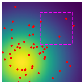
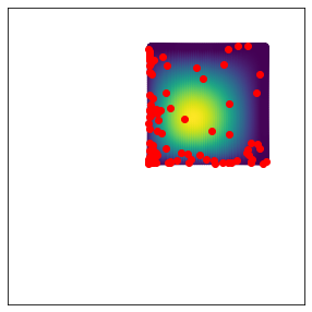
Figure 1: Our interpretable normalizing flow policy. Left: Environment, the agent should reach the star while avoiding dangerous obstacles and walls. Middle: A single flow step maps the initially unbounded policy distribution into the region satisfying the constraint (magenta rectangle), action samples are plotted in red. Right: The final policy distribution has support only over the allowed region.

II Background

We begin by formally defining the type of constrained RL problems we wish to solve and provide the relevant methods underlying our proposed approach.

II-A Constrained Reinforcement Learning

Reinforcement learning problems are formalized as Markov Decision Processes (MDP)s. An MDP is a tuple $\mathcal{M}\equiv\langle\mathcal{S,A},r,\rho,\gamma\rangle$, where $\mathcal{S}$ and $\mathcal{A}$ respectively denote the $n$- and $m$-dimensional state- and action-space, $r:\mathcal{S}\times\mathcal{A}\to\mathbb{R}$ is the scalar-valued reward function, $\rho:\mathcal{S}\times\mathcal{A}\to\mathcal{S}$ are the discrete-time transition dynamics, and $\gamma\in[0,1]$ is a discount factor. The goal in RL is to find a policy $\pi:\mathcal{S}\times\mathcal{A}\to[0,1]$ that maximizes the total expected return

$$J(\pi)=\mathbb{E}_{(\tau\sim\pi)}\Big{[}{\sum_{t=0}^{\infty}\gamma^{t}r(\mathbf{s}_{t},\mathbf{a}_{t})}\Big{]},$$ (1)

where $\mathbf{s}_{t}\in\mathcal{S}$ and $\mathbf{a}_{t}\in\mathcal{A}$ and $(\tau\sim\pi)$ is shorthand for denoting trajectories $\tau$ with actions sampled from the policy and states samples from the MDP’s transition dynamics. Constrained RL additionally assumes a number of constraints $c_{1},\dots,c_{K}$ that limit policy search for Eq. (1). In this paper, we consider instantaneous constraints [1], resulting in the constrained optimization

$$\underset{\pi}{\max}\ J(\pi)\ \text{s.t.}\ c_{k}(\mathbf{s}_{t},\mathbf{a}_{t})\leq\varepsilon_{k}\ \forall k\in\{1,\dots,K\},\forall t,$$ (2)

where $\varepsilon_{k}$ is a pre-defined threshold for the constraint function $c_{k}:\mathcal{S}\times\mathcal{A}\to\mathbb{R}$.

A popular approach for solving such constrained RL problems relies on Lagrangian relaxation, which introduces Lagrange multipliers $\lambda$ to make for an approximation of the above constrained optimization. The Lagrangian relaxation of Eq. (2) is given by

$$J(\pi,\lambda)=\mathbb{E}_{(\tau\sim\pi)}\Big{[}\sum_{t=0}^{\infty}\gamma^{t}r(\mathbf{s}_{t},\mathbf{a}_{t})-\sum_{k=1}^{K}\lambda_{k}\big{(}c_{k}(\mathbf{s}_{t},\mathbf{a}_{t})-\varepsilon_{k})\big{)}\Big{]}.$$ (3)

Optimizing the objective in Eq. 3 with dual gradient descent, as in [10, 11], results in an agent that approximately solves Eq. (2). Other approaches to constrained RL involve projections, that learn to map actions into the allowed set [2, 12]. These methods often require an expensive optimization step, e.g. [12] [12] have to solve a quadratic problem to map each action into the safe set. Shielding approaches [4, 13, 14] ensure that only allowed actions are executed, however, they require access to the transition model or modify the environment directly to enforce constraints. Importantly, solely rejecting actions that violate constraints does not suffice, since this would lead to biased gradient estimates [13, 15].

In this paper, we instead exploit the following, useful property of instantaneous constraints, namely, the fact that they separate the per-state action space into two sub-spaces: $\mathcal{A}_{\varphi,k}^{\mathbf{s}}$, which contains all actions that satisfy constraint $k$ in state $\mathbf{s}$ and $\mathcal{A}_{\psi,k}^{\mathbf{s}}$, that contains the actions that violate constraint $k$ in state $\mathbf{s}$. We define $\mathcal{A}_{\varphi}^{\mathbf{s}}=\mathcal{A}_{\varphi,1}^{\mathbf{s}}\cap\dots\cap\mathcal{A}_{\varphi,K}^{\mathbf{s}}$ as the intersection of all allowed constraint regions for state $\mathbf{s}$. Therefore, instantaneous constraints can be used to induce a new MDP $\mathcal{M}_{\varphi}$ [16, 17] that uses $\mathcal{A}_{\varphi}^{\mathbf{s}}$ as per-state action-space and leaves everything else as in the original MDP $\mathcal{M}$. Theoretically, $\mathcal{M}_{\varphi}$ can then be optimized with regular RL algorithms that then satisfy the constraints, even during learning, by construction. In practice, this requires sample access to $\mathcal{A}_{\varphi}$ or a mapping from $\mathcal{A}$ to $\mathcal{A}_{\varphi}$. In this work we consider the former approach by exploiting mapping functions for instantaneous constraints and show how they can be integrated into Soft Actor-Critic (SAC) (or other policy-gradient algorithms) by means of normalizing flow policies.

II-B Soft Actor-Critic

Soft Actor-Critic [18, 19] is a model-free RL algorithm for MDPs with continuous state and action spaces. SAC maximizes the following maximum-entropy objective [20], which augments Eq. (1) with the policy’s entropy $\mathcal{H}=\mathbb{E}_{\mathbf{a}\sim\pi(\cdot\mid\mathbf{s})}[-\log\pi(\mathbf{a}\mid\mathbf{s})]$,

$$J_{\text{ME}}(\pi)=\mathbb{E}_{(\mathbf{a}_{t}\sim\pi),(\mathbf{s}_{t}\sim\rho)}\Big{[}{\sum_{t=0}^{\infty}\gamma^{t}r(\mathbf{s}_{t},\mathbf{a}_{t})+\alpha\mathcal{H}(\pi(\cdot\mid\mathbf{s}_{t})}\Big{]},$$ (4)

where $\alpha$ balances the entropy and the reward objective. SAC learns an on-policy critic Q-function, $Q_{\theta}$, with parameter $\theta$, by optimizing for Bellman consistency

$$J_{Q}(\theta)=\mathbb{E}_{\mathcal{D}}\Big{[}\frac{1}{2}\Big{(}Q_{\theta}(\mathbf{s}_{t},\mathbf{a}_{t})-\big{(}r(\mathbf{s}_{t},\mathbf{a}_{t})+\gamma V_{\bar{\theta}}(\mathbf{s}_{t+1})\big{)}\Big{)}^{2}\Big{]},$$ (5)

where $\mathbf{s}_{t},\mathbf{a}_{t}$, and $\mathbf{s}_{t+1}$ are sampled from a replay buffer $\mathcal{D}$, $V_{\bar{\theta}}=\mathbb{E}_{(\mathbf{a}_{t+1}\sim\pi})[Q_{\bar{\theta}}(\mathbf{s}_{t+1},\mathbf{a}_{t+1})-\alpha\log\pi(\mathbf{a}_{t}\mid\mathbf{s}_{t}))]$ is the maximum-entropy on-policy state-value function, and $\bar{\theta}$ is a target network [21] parameter. With respect to the actor, SAC employs an infinite-support, unimodal Gaussian with diagonal covariance and mean given by a policy network, $\pi_{\phi}$, which is parameterized by $\phi$. The policy network update makes use of the reparametrization trick and backpropagates through the critic

$$J_{\pi}(\phi)=\mathbb{E}_{(\mathbf{s}_{t}\sim\mathcal{D})}\Big{[}\mathbb{E}_{(\mathbf{a}_{t}\sim\pi_{\phi})}\big{[}\alpha\log\pi_{\phi}(\mathbf{a}_{t}\mid\mathbf{s}_{t})-Q_{\theta}(\mathbf{s}_{t},\mathbf{a}_{t})\big{]}\Big{]},$$ (6)

to increase the likelihood of actions that have high Q-values. To bound the action space, SAC squashes the Gaussian action samples with the hyperbolic tangent function to obtain the final actor distribution, which is referred to as a squashed Gaussian distribution. The density of the squashed Gaussian can be obtained using the change of variables formula. Given a random variable $\mathbf{a}$, its density $\pi(\mathbf{a}\mid\mathbf{s})$, and an invertible function $f$, the density of the transformed random variable $\mathbf{a^{\prime}}=f(\mathbf{a})$ is given by

$$\pi(\mathbf{a^{\prime}}\mid\mathbf{s})=\pi(\mathbf{a}\mid\mathbf{s})\left|\det\frac{\partial f^{-1}}{\partial\mathbf{a^{\prime}}}\right|=\pi(\mathbf{a}\mid\mathbf{s})\left|\det\frac{\partial f}{\partial\mathbf{a}}\right|^{-1},$$ (7)

where $f^{-1}$ is the inverse of the transformation $f$. Eq. (7) is used to obtain the policy’s log-density in Eq. (5) and (6). Importantly, while SAC uses the hyperbolic tangent for $f$ to bound the action space, the change of variables formula allows for any invertible function. This prompts the key idea behind our method: If we can express instantaneous constraints in terms of invertible functions on $\mathcal{A}$, we can directly transform $\mathcal{A}$ into $\mathcal{A}_{\varphi}$ on a per-state basis and learn optimal policies directly in $\mathcal{M}_{\varphi}$. In the next section, we show how this idea can be generalized to multiple constraints and that the resulting distribution corresponds exactly to what is known as a normalizing flow policy.

III Constrained Normalizing Flow Policies

Normalizing Flows (NFs) [8] are models for variational inference that transform a simple, initial density (e.g. Gaussians) into a complex posterior distribution by applying a sequence of learned, invertible transformations to the original density. A degenerate, one-step NF with only one transformation $f$ is referred to as a flow and the resulting density is given by Eq. (7). In this sense, unmodified SAC applies a one-step NF to obtain the density of the squashed Gaussian distribution, which has no parametric form. A proper NF refers to the composition of multiple (learned) transformations on the random variable $\mathbf{a}$, with $\mathbf{a}_{M}=f_{M}(f_{M-1}(\dots f(\mathbf{a}))$, in which case Eq. (7) is successively applied to yield the (log-) density

$$\log\pi(\mathbf{a}_{M}\mid\mathbf{s})=\log\pi(\mathbf{a}\mid\mathbf{s})-\sum_{m=1}^{M}\log\left|\det\frac{\partial f_{m}}{\partial\mathbf{a}_{m-1}}\right|.$$ (8)

As shown in [8] NFs are highly flexible and can approximate complex, multi-modal posterior distributions. By viewing the squashed Gaussian distribution in SAC as the result of single flow step, it is intuitive to replace the squashed Gaussian with more expressive, multi-modal NFs. When these transformations are learned, the resulting architecture is referred to as a normalizing flow policy [9].

Normalizing flow policies are primarily used to obtain more expressive policy distributions, which reportedly improves exploration and learning efficiency [9, 22, 23]. We find two related works investigating constrained RL problems with the help of flow-based policies. [24] [24] also focus on RL problems with instantaneous constraints, as in Eq. (2), and propose FlowPG to learn an invertible mapping from $\mathcal{A}$ to $\mathcal{A}_{\varphi}$, i.e. to map any given action into the per-state allowed sub-space. FlowPG requires a large dataset of actions in $\mathcal{A}_{\varphi}^{\mathbf{s}}$ for each state $\mathbf{s}$, which the authors propose to obtain via an expensive, initial Hamiltonian Monte-Carlo (HMC) [25] step. [26] [26] instead focus on feasibility constraints in large, discrete action spaces and learn an Argmax Flow [27] network that generates samples from the feasible, categorical action distribution. To ensure that only allowed actions are executed, the authors include a rejection sampling step that may fail if the feasible set is small. The key difference between previous works on constrained flow-based policies and our method is that we, instead of learning the $M$ transformations from data, propose to construct the transformation functions analytically, considering domain knowledge and constraint functions. We describe our approach to this in the next section.

IV Method

In this paper, we consider RL problems with instantaneous constraints, as in Eq. (2), with the constraints defined on the MDPs state-action space. We propose to analytically construct functions that map into the per-state, per-constrain allowed action subspace $\mathcal{A}_{\varphi,k}^{\mathbf{s}}$. More formally, we assume $K$ instantaneous constraint functions $c_{1}(\mathbf{s,a}),\dots,c_{K}(\mathbf{s,a})$ with corresponding thresholds $\varepsilon_{1},\dots,\varepsilon_{K}$, which induce $\mathcal{A}_{\varphi,1}^{\mathbf{s}},\dots,\mathcal{A}_{\varphi,K}^{\mathbf{s}}$, the per-state $\mathbf{s}$, per-constrain $k$ allowed action sub-spaces. We now make a relatively strong, simplifying assumption: We assume that all $\mathcal{A}_{\varphi,k}^{\mathbf{s}}$ are convex because it is relatively easy to find invertible transformations that map points into the convex sets. So far, we developed functions for mapping or squashing into hypercubes, hyperspheres, and ellipsoids (the former could correspond to percentiles on learned Gaussians), but we hypothesize that there are invertible squashing functions for more complex polytopes. Fig. 2 illustrates these invertible squashing functions in 2D. While the exploration of non-convex, invertible squashing functions is out of scope for this paper, we note that multiple simple, convex constraints can be combined to induce a complex, overall constraint on the agent.

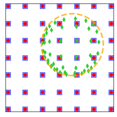
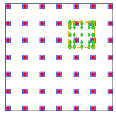
Figure 2: Invertible mapping functions. Exemplary constraint regions are drawn in orange . These functions map from the unbounded domain into the constraint region, i.e. $f(\includegraphics[height=7.20007pt]{imgs/particle.png})\to\includegraphics[height=7.20007pt]{imgs/squashed_particle.png}$. The inverse function maps from the constraint region back to the unbounded domain, i.e. $f^{-1}(\includegraphics[height=7.20007pt]{imgs/squashed_particle.png})\to\includegraphics[height=7.20007pt]{imgs/unsquashed_particle.png}=\includegraphics[height=7.20007pt]{imgs/particle.png}$.

To provide a concrete example of our method, consider two constraint function $c_{1}(\mathbf{s,a})$ and $c_{2}(\mathbf{s,a})$ with corresponding $\varepsilon_{1},\varepsilon_{2}$, whose convex sub-spaces are $\mathcal{A}_{\varphi,1}^{\mathbf{s}}$ and $\mathcal{A}_{\varphi,2}^{\mathbf{s}}$ in each state $\mathbf{s}$, and the corresponding invertible functions $f_{1}^{\mathbf{s}}$ and $f_{2}^{\mathbf{s}}$ that respectively map points into $\mathcal{A}_{\varphi,1}^{\mathbf{s}}$ and $\mathcal{A}_{\varphi,2}^{\mathbf{s}}$. By assuming that $f_{1}^{\mathbf{s}}$ and $f_{2}^{\mathbf{s}}$ are known (or can be constructed), we can directly use these functions to construct an interpretable, constrained NF policy by inserting them into Eq. (8). The resulting NF policy will sequentially map the initially unbounded action-space into the sub-space allowed by the constraints, such that the final distribution only has support over $\mathcal{A}_{\varphi,1}^{\mathbf{s}}\cap\mathcal{A}_{\varphi,2}^{\mathbf{s}}$, the intersection of all constraint subsets. This is the core idea behind our method, which is applicable to instantaneous constraints for which we know or can analytically construct the mapping functions. The consequences of this modelling can be seen in Fig. 3. As shown, depending on the state and the constraint, the squashing functions are restrictive or largely permissive. The final policy distribution is obtained in an interpretable manner since each transformation in the normalizing flow aligns the policy with respect to one of the constraints. This approach can trivially be extended to $K>2$ constraints, since simply the range of the summation in Eq. 8 increases from $2$ to $K$.

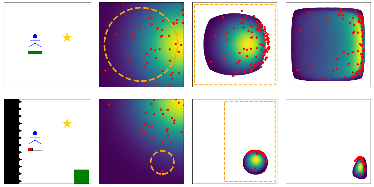
Figure 3: Two normalizing flows. Top: Permissive constraints, no obstacles are in close proximity and the battery is fully charged. Bottom: Restrictive constraints, the agent is close to an obstacle and its battery is almost empty. The green rectangle indicates a charging station.

Note, that the order in which we apply our transformations matters since the mapping functions are or can be non-linear, meaning we have $f_{1}^{\mathbf{s}}(f_{2}^{\mathbf{s}}(\mathbf{a}))\neq f_{2}^{\mathbf{s}}(f_{1}^{\mathbf{s}}(\mathbf{a}))$. The normalizing flow generally maps into the intersection of $\mathcal{A}_{\varphi,1}^{\mathbf{s}}$ and $\mathcal{A}_{\varphi,2}^{\mathbf{s}}$, however, the resulting distribution can look different, depending on the order of transformations. This can be used to impose a notion of priority on the constraints: For each constraint $l$ and the corresponding transformation $f_{l}$ that comes before $k$ in the flow sequence, the intermediate $\mathcal{A}_{\varphi,l}^{\mathbf{s}}$ will be mapped into $\mathcal{A}_{\varphi,k}^{\mathbf{s}}$ by the subsequent transformation $f_{k}$ which may not overlap with $\mathcal{A}_{\varphi,l}^{\mathbf{s}}$. This is a desirable property because it ensures that even if constraints are incompatible, i.e. when $\mathcal{A}_{\varphi,1}^{\mathbf{s}}\cap\mathcal{A}_{\varphi,2}^{\mathbf{s}}=\emptyset$, our NF policy will always map into the sub-space of the higher-priority constraint, whose transformation is applied after that of the lower-priority constraints.

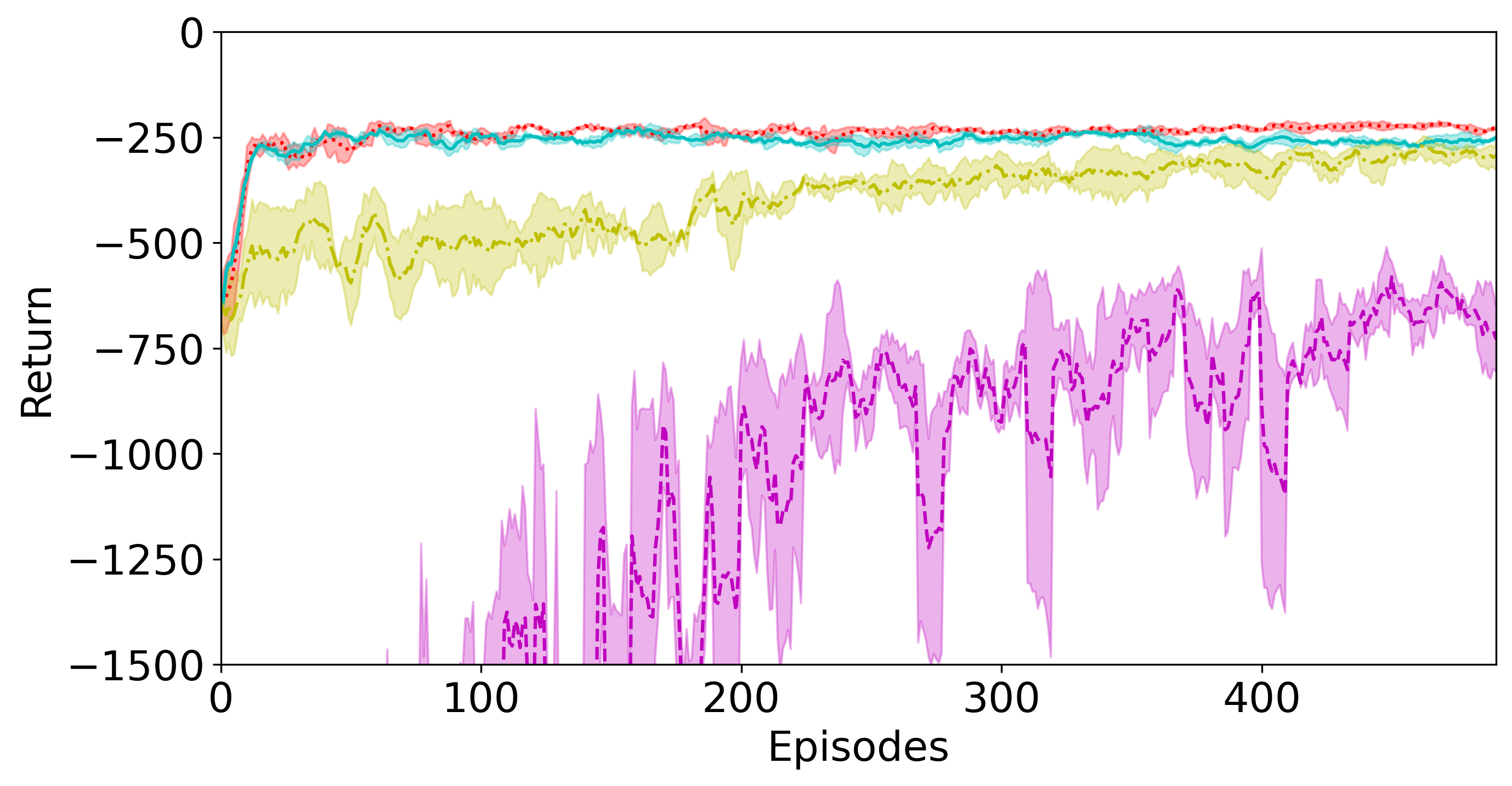
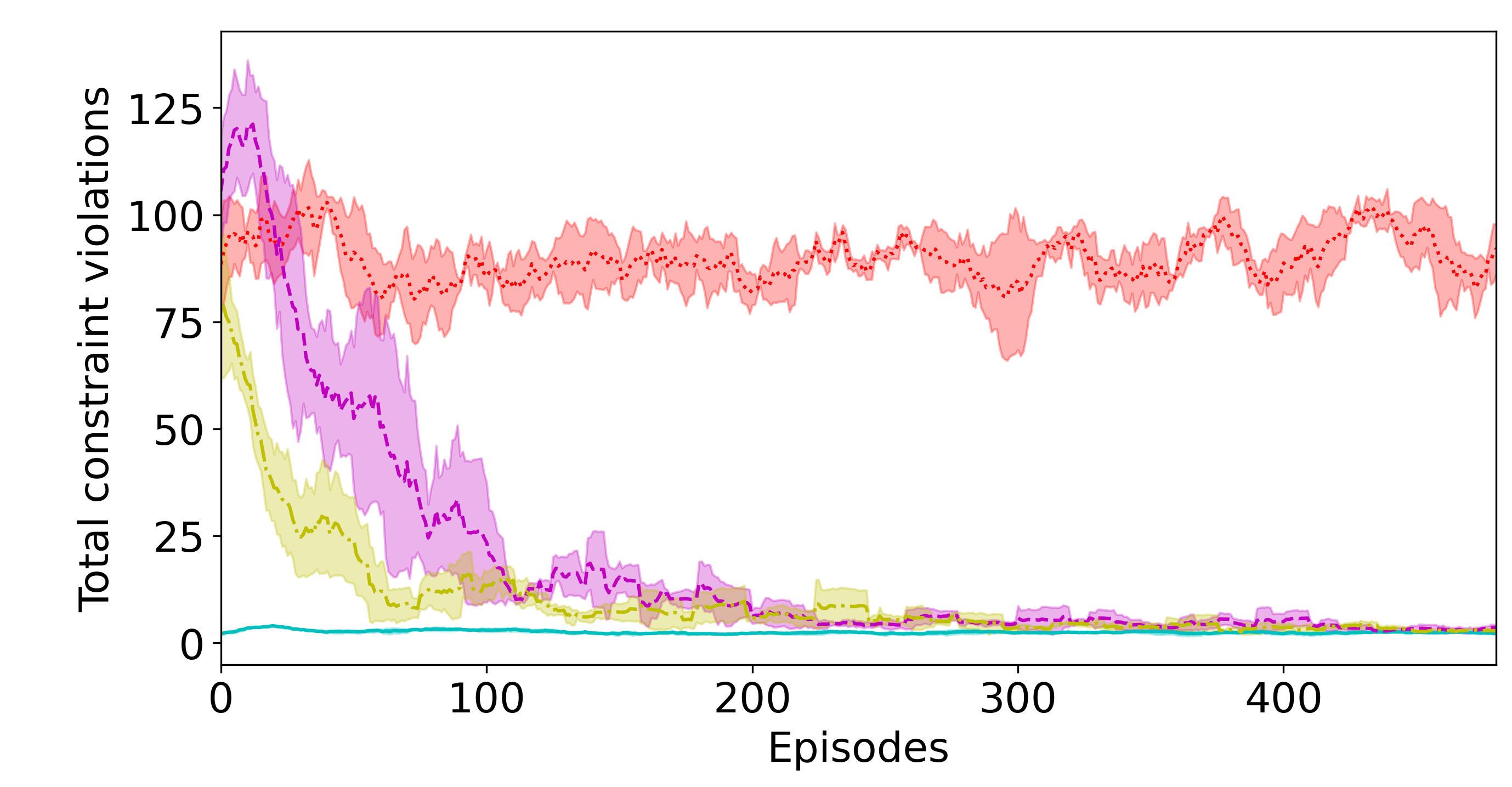
Figure 4: Baseline comparison in a constrained 2D point navigation environment. Left: Our agent (CNFP) learns the task as quickly as the unconstrained agent since it optimizes the same, smooth and dense reward function while benefiting from a reduced search space. Right: Unlike other baselines, our agent maintains quasi-perfect constraint satisfaction throughout learning. The experiment was repeated three times with varying random seeds, the shaded area corresponds to one standard deviation around the mean.

The concrete steps of our method can be summarized as follows: Given an RL problem with a set of instantaneous, convex constraints $c_{1}(\mathbf{s,a})\leq\varepsilon_{1},\dots,c_{K}(\mathbf{s,a})\leq\varepsilon_{K}$, find the corresponding invertible functions $f_{1},\dots,f_{K}$ that map into $\mathcal{A}_{\varphi,1},\dots\mathcal{A}_{\varphi,K}$. Next, order the constraints by domain-specific priority, e.g. $c_{1}\succ\dots\succ c_{K}$. Insert the constraint mapping function into Eq. (8), such that the lowest-priority constraint transformation $f_{K}$ is applied first and the highest priority constraint transformation, $f_{1}$ is applied last. Use the resulting normalizing flow to compute the log-density of the constrained NF policy, e.g. in Eq. (5) and Eq. (6) for SAC or other policy-gradient algorithms. In the next section, we demonstrate this approach in a simplistic 2D environment as proof-of-concept.

V Experiments

V-A Environment

We empirically validate our method on a constrained 2D point navigation problem, where the agent has to reach a target coordinate while constrained to avoiding obstacles and keeping the battery charge above 20%. At each step, the battery depletes by 1% but can be charged by visiting a charging station, with one charging station placed at each side of the rectangular environment. The outside walls as well as a centrally-placed rectangle provide the static obstacles the agent should avoid colliding with. The central obstacle ensures that the direct path to the goal is obstructed, such that an unconstrained agent will inquire high constraint violations. The observation vector is in $\mathbb{R}^{5}$ and corresponds to the agent’s current 2D coordinate, the current battery level, and the 2D goal coordinate. Actions correspond to translations in the 2D plane. The reward function is dense and corresponds to the negative Euclidean distance between the agent and the target coordinate, encouraging the agent to greedily navigate towards the goal. When the agent reaches the goal, a bonus of $10$ reward is provided and a new goal position is randomly sampled. There are no terminal states, however, episodes are truncated and the environment resets after 100 steps. The constraints are modelled as indicator functions. The constraint for obstacle avoidance, $\mathbb{I}_{O}(\mathbf{s,a})$ maps to one if executing $\mathbf{a}$ in $\mathbf{s}$ would lead to a collision with an obstacle. The constraint function for the battery level, $\mathbb{I}_{B}(\mathbf{s,a})$ maps to one if executing $\mathbf{a}$ in $\mathbf{s}$ leads to the battery falling beneath the 20% threshold. Both corresponding constraint thresholds, $\varepsilon_{O},\varepsilon_{B}$ are set to $0$.

V-B Methods

For our constrained normalizing flow policy (CNFP), we analytically construct the invertible functions $f_{B}^{\mathbf{s}},f_{O}^{\mathbf{s}}$ for mapping into $\mathcal{A}_{\varphi,B}^{\mathbf{s}}$ and $\mathcal{A}_{\varphi,O}^{\mathbf{s}}$, i.e., the per-state action-subspaces that keep the battery and obstacle-avoidance constraints satisfied. Due to the rectangular layout of the environment we model $f_{O}^{\mathbf{s}}$, the function for mapping into $\mathcal{A}_{\varphi,O}^{\mathbf{s}}$, with the rectangle squashing function (right side of Fig. 2). The dimensions of the rectangular constraint region are inferred from the environment and the agent’s current position, just like $\mathbb{I}_{O}(\mathbf{s,a})$ itself. If the agent is sufficiently far from all obstacles, this constraint simply bounds the action space to $[-1,1]$, however, in closer proximity to the obstacle, the bound becomes tighter and excludes those actions that would lead to collisions. The battery constraint mapping function $f_{B}^{\mathbf{s}}$ is modelled with the circular squashing function (left side of Fig. 2). If the battery level is sufficiently high, the circle is zero-centred and has a large radius. As the battery level decreases, the radius becomes smaller and the circle is placed at the closest charging station. Thus, if the battery level is low, the agent is automatically “pulled” to the closest charging station. We define the priority order of these constraints as $\mathbb{I}_{O}\succ\mathbb{I}_{B}$, meaning avoiding obstacles is assigned higher priority than keeping the battery fully charged. Our constrained normalizing flow policy thus corresponds to $\mathbf{a^{\prime}}=f_{O}^{\mathbf{s}}(f_{B}^{\mathbf{s}}(\mathbf{a}\sim\pi(\cdot\mid\mathbf{s})))$.

In addition to our CNFP agent, we include the following baselines. Firstly, we include an unconstrained SAC agent that maximizes the reward function while disregarding the constraints entirely. This agent provides a baseline for constraint violations caused when optimizing only the reward. Next, we include a SAC agent where constraint violations are punished via the reward function. For this agent, we modify the dense reward function to yield a large negative penalty, $-100$, whenever at least one of the two constraints is violated. Behaving optimal with respect to this reward function is equivalent to solving the task while respecting the constraints. Lastly, we include a Sac-Lagrangian agent that optimizes Eq. 3, as described in [10, 11].

V-C Results

Our main result is shown in Fig. 4, with two main insights. Firstly, our CNFP agent learns to solve the goal-navigation task optimally within only a few episodes, as can be seen on the left side in Fig. 4. This can be explained by two observations. On the one hand, CNFP optimizes the same smooth and dense reward function as the unconstrained baseline agent, which makes learning easy. This is not the case for the reward penalty or Lagrangian agents. Although the Lagrangian agent also optimizes the same smooth and dense reward function as the unconstrained baseline and CNFP, it also has to consider the constraint violations in the actor objective, which results in a harder objective for policy search. As a consequence, the Lagrangian agent converges only slowly to near-optimal performance. For the reward penalty agent, the reward function is still dense but it is not smooth since it is dominated by the large penalties raised due to constraint violations. This makes learning the task harder. The reward penalty agent did therefore only learn to avoid constraint-violating actions, but did not converge to an optimal level of performance within the number of episodes of this experiment. The quick convergence of our CNFP agent to an optimal level of task return can further be explained by a reduced search space. The behaviors accounting for the obstacle avoidance and battery-level constraints do not have to be learned, since we can exploit domain knowledge to encode them into the agent via the transformation functions $f_{O}^{\mathbf{s}}$ and $f_{B}^{\mathbf{s}}$. No matter where the policy network places the initial Gaussian $\mathcal{N}(\mu_{\phi},\Sigma_{\phi})$ and which action is sampled, if the agent is close to an obstacle, the sampled action (and corresponding density) will be transformed by $f_{O}^{\mathbf{s}}$ in such a way that a collision is no longer possible (e.g. Fig. 1 and Fig 3). The same is true for the battery constraint. Therefore, our agent’s learning objective is solely the maximization of task return, while the constraints are satisfied by construction of the constrained normalizing flow policy and do not require any plasticity in the policy network.

The second insight is that, as can be seen on the right side of Fig. 4, our CNFP agent maintains quasi-perfect constraint satisfaction throughout the entirety of training. This is expected, since correct mapping functions $f_{O}^{\mathbf{s}}$ and $f_{B}^{\mathbf{s}}$ should never allow constraint-violating actions to be executed. As revealed through the unconstrained agent, solving the task optimally without accounting for constraints results in many constraint-violating actions. Both the reward penalty and the Lagrangian agent drastically decrease the number of constraint violations throughout training, however, both inquire a high number of violations at the beginning of training. At the same time, for these agents, the reduction in constraint violations comes at a cost: The reward penalty agent learns overly pessimistic behaviour which indeed results in few violations, however, at the cost of drastic performance degradation in terms of task return. The Lagrangian agent converges to a similar level of constraint violation as the reward penalty agent while achieving better task return, although only reaching near-optimal performance at the very end of training. Thus, to summarize the results so far, our CNFP agent is the only one to maintain perfect constraint satisfaction through training while achieving task return levels as quickly as and on par with an unconstrained, optimal agent.

Lastly, we want to highlight again the interpretable nature of our model. Unlike all other baselines that learn a single, monolithic policy, our CNFP policy is interpretable, since each step in the normalizing flow can be visualized and used to explain the agent’s behaviour. While the initial, unbounded policy distribution is still obtained from a black-box neural network, it can be explained how this distribution is transformed to ensure that the agent respects the given constraints. This can reveal flaws in the construction of the constraint mapping functions, i.e. it can be seen when a mapping function is to permissive and allows the execution of unsafe actions. It can therefore be explained how an unsafe action in particular state must be transformed to ensure alignment w.r.t each constraint. This is not the case for our baseline methods that learn monolithic policies with constraints simply moved into the learning objective.

VI Conclusion and future work

In this paper, we have shown how normalizing flows can be used to obtain interpretable policies for constrained reinforcement learning problems. Our experiments revealed a favourable comparison against baselines with respect to task return and constraint violations, with additional benefits in and beyond interpretability: The action-space transformation functions, which constitute the normalizing flow, make for a form of knowledge transfer by encoding desired behaviour in terms of constraints on the action space. Then, the constraints do not have to be considered in the reward function and value estimates, which leaves a simple optimization objective that can be learned quickly. As the most important future work, we see the development of non-convex transformation functions, to broaden the applicability of our approach to more complex scenarios, as well as the integration of learnable mapping functions for complex constraints. In this context, it might be worthwhile to explore differentiable constraint functions, as in  [13], which are susceptible to learning with normalizing flows.

References

- [1] Yongshuai Liu, Avishai Halev and Xin Liu “Policy learning with constraints in model-free reinforcement learning: A survey” In The 30th international joint conference on artificial intelligence (ijcai), 2021
- [2] Joshua Achiam, David Held, Aviv Tamar and Pieter Abbeel “Constrained policy optimization” In International conference on machine learning, 2017, pp. 22–31 PMLR
- [3] Eitan Altman “Constrained Markov decision processes” 1st Edition. Routledge, 1999
- [4] Mohammed Alshiekh et al. “Safe reinforcement learning via shielding” In Proceedings of the AAAI conference on artificial intelligence 32.1, 2018
- [5] Stuart J Russell and Andrew Zimdars “Q-decomposition for reinforcement learning agents” In Proceedings of the 20th International Conference on Machine Learning (ICML-03), 2003, pp. 656–663
- [6] Zoe Juozapaitis et al. “Explainable reinforcement learning via reward decomposition” In IJCAI/ECAI Workshop on explainable artificial intelligence, 2019
- [7] Finn Rietz et al. “Hierarchical goals contextualize local reward decomposition explanations” In Neural Computing and Applications 35.23 Springer, 2023, pp. 16693–16704
- [8] Danilo Rezende and Shakir Mohamed “Variational inference with normalizing flows” In International conference on machine learning, 2015, pp. 1530–1538 PMLR
- [9] Patrick Nadeem Ward, Ariella Smofsky and Avishek Joey Bose “Improving exploration in soft-actor-critic with normalizing flows policies” In arXiv preprint arXiv:1906.02771, 2019
- [10] Sehoon Ha et al. “Learning to walk in the real world with minimal human effort” In arXiv preprint arXiv:2002.08550, 2020
- [11] Qisong Yang, Thiago D Simão, Simon H Tindemans and Matthijs TJ Spaan “WCSAC: Worst-case soft actor critic for safety-constrained reinforcement learning” In Proceedings of the AAAI Conference on Artificial Intelligence 35.12, 2021, pp. 10639–10646
- [12] Tu-Hoa Pham, Giovanni De Magistris and Ryuki Tachibana “Optlayer-practical constrained optimization for deep reinforcement learning in the real world” In 2018 IEEE International Conference on Robotics and Automation (ICRA), 2018, pp. 6236–6243 IEEE
- [13] Wen-Chi Yang, Giuseppe Marra, Gavin Rens and Luc De Raedt “Safe Reinforcement Learning via Probabilistic Logic Shields” Main Track In Proceedings of the Thirty-Second International Joint Conference on Artificial Intelligence, IJCAI-23 International Joint Conferences on Artificial Intelligence Organization, 2023, pp. 5739–5749 DOI: 10.24963/ijcai.2023/637
- [14] Nathan Hunt et al. “Verifiably safe exploration for end-to-end reinforcement learning” In Proceedings of the 24th International Conference on Hybrid Systems: Computation and Control, 2021, pp. 1–11
- [15] Po-Wei Chou, Daniel Maturana and Sebastian Scherer “Improving stochastic policy gradients in continuous control with deep reinforcement learning using the beta distribution” In International conference on machine learning, 2017, pp. 834–843 PMLR
- [16] Finn Rietz, Stefan Heinrich, Erik Schaffernicht and Johannes Andreas Stork “Prioritized Soft Q-Decomposition for Lexicographic Reinforcement Learning” In arXiv preprint arXiv:2310.02360, 2023
- [17] Hengrui Zhang, Youfang Lin, Sheng Han and Kai Lv “Lexicographic Actor-Critic Deep Reinforcement Learning for Urban Autonomous Driving” In IEEE Transactions on Vehicular Technology IEEE, 2022
- [18] Tuomas Haarnoja, Aurick Zhou, Pieter Abbeel and Sergey Levine “Soft actor-critic: Off-policy maximum entropy deep reinforcement learning with a stochastic actor” In International conference on machine learning, 2018, pp. 1861–1870 PMLR
- [19] Tuomas Haarnoja et al. “Soft actor-critic algorithms and applications” In arXiv preprint arXiv:1812.05905, 2018
- [20] Brian D Ziebart, Andrew L Maas, J Andrew Bagnell and Anind K Dey “Maximum entropy inverse reinforcement learning.” In Aaai 8, 2008, pp. 1433–1438 Chicago, IL, USA
- [21] Volodymyr Mnih et al. “Human-level control through deep reinforcement learning” In nature 518.7540 Nature Publishing Group, 2015, pp. 529–533
- [22] Olivier Delalleau, Maxim Peter, Eloi Alonso and Adrien Logut “Discrete and continuous action representation for practical rl in video games” In arXiv preprint arXiv:1912.11077, 2019
- [23] Bogdan Mazoure et al. “Leveraging exploration in off-policy algorithms via normalizing flows” In Conference on Robot Learning, 2020, pp. 430–444 PMLR
- [24] Janaka Chathuranga Brahmanage, Jiajing Ling and Akshat Kumar “FlowPG: Action-constrained Policy Gradient with Normalizing Flows” In arXiv preprint arXiv:2402.05149, 2024
- [25] Michael Betancourt “A conceptual introduction to Hamiltonian Monte Carlo” In arXiv preprint arXiv:1701.02434, 2017
- [26] Changyu Chen et al. “Generative Modelling of Stochastic Actions with Arbitrary Constraints in Reinforcement Learning” In arXiv preprint arXiv:2311.15341, 2023
- [27] Emiel Hoogeboom et al. “Argmax flows and multinomial diffusion: Learning categorical distributions” In Advances in Neural Information Processing Systems 34, 2021, pp. 12454–12465