Optimal Beamforming for Bistatic MIMO Sensing

Abstract

This paper considers the beamforming optimization for sensing a point-like scatterer using a bistatic multiple-input multiple-output (MIMO) orthogonal frequency-division multiplexing (OFDM) radar, which could be part of a joint communication and sensing system. The goal is to minimize the Cramér-Rao bound on the target position’s estimation error, where the radar already knows an approximate position that is taken into account in the optimization. The optimization allows for beamforming with more than one beam per subcarrier. Optimal solutions for the beamforming are discussed for known and unknown channel gain. Numerical results show that beamforming with at most one beam per subcarrier is optimal for certain parameters, but for other parameters, optimal solutions need two beams on some subcarriers. In addition, the degree of freedom in selecting which end of the bistatic radar should transmit and receive is considered.

I Introduction

In this paper, we consider a bistatic multiple-input multiple-output (MIMO) orthogonal frequency-division multiplexing (OFDM) radar that is sensing a point-like target. There is a large body of literature that only considers bistatic systems or networks with single transmit and receive antennas at each node, see e.g., [1, 2, 3, 4]. Bistatic radars are particularly interesting in the context of joint communication and sensing (JC&S) in cellular systems with base station cooperation. We aim to optimize the beamforming and compare the estimation performance measured by the Cramér-Rao bound (CRB) on the target position’s estimation error with known and unknown channel gain. Beamforming can improve both the signal-to-noise ratio (SNR) and allows for spatial filtering. The work was inspired by [5], where a single beam is used for position estimation based on the azimuth angles of arrival (AoA) and departure (AoD) in a single-frequency system / on a single subcarrier. We extend this by also considering the delay between transmitter and receiver for the position estimation and more than one beam per subcarrier in an OFDM system. In the following section, a system model based on the azimuth AoA and AoD and the delay between transmitter and receiver is used, which is valid in the far-field. The optimization of the beamforming and properties of optimal solutions are discussed, including the degree of freedom in selecting which end of the bistatic radar should transmit and receive. Further, the influence of a known channel gain is considered.

Notation: lowercase bold letters denote vectors, uppercase bold letters matrices. $\bm{A}^{T}$, $\bm{A}^{\ast}$, $\bm{A}^{H}$, $\lVert\bm{a}\rVert$ and $\operatorname{tr}(\bm{A})$ correspond to the transposed, the complex conjugate, the Hermitian, the Euclidean norm and the trace respectively. $\operatorname{diag}(d_{1},\dotsc,d_{N})$ denotes the diagonal matrix with $d_{1}$ to $d_{N}$ on its diagonal. $\bm{0}$ and $\bm{I}$ are the zero vector/matrix and identity matrix. $\mathcal{N}_{\mathbb{C}}(\mu,\sigma^{2})$ denotes a circularly-symmetric complex Gaussian distribution with mean $\mu$ and variance $\sigma^{2}$. $\operatorname{E}[X]$ denotes the expectation of the random variable $X$.

II System Model

Figure 1: Geometry for bistatic sensing.

The following model is based on the framework presented in [6]. Consider a bistatic MIMO OFDM radar supporting $P$ subcarriers with a transmitter with $N_{\mathrm{T}}$ antennas located at the 2D position $\bm{p}_{\mathrm{T}}$ and a receiver with $N_{\mathrm{R}}$ antennas located at $\bm{p}_{\mathrm{R}}$ sensing a target at position $\bm{p}_{\mathrm{S}}^{T}=\begin{bmatrix}x_{\mathrm{S}},y_{\mathrm{S}}\end{bmatrix}$, see Fig. 1. $d_{\mathrm{TS}}$ and $d_{\mathrm{SR}}$ are the distances between scatterer and transmitter and scatterer and receiver.

The received signal on the $p$-th subcarrier $\bm{y}[p]\in\mathbb{C}^{N_{\mathrm{R}}}$ in an additive white Gaussian noise (AWGN) channel is given by

$$\bm{y}[p]=\bm{m}[p]+\bm{\eta}[p],\quad\bm{\eta}[p]\sim\mathcal{N}_{\mathbb{C}}(\bm{0},\sigma_{\eta}^{2}\bm{I}),$$ (1)

$$\bm{m}[p]=\sum\limits_{l=0}^{1}h_{l}\bm{a}_{\mathrm{R},l}[p](\tilde{\theta}_{\mathrm{R},l})\bm{a}_{\mathrm{T},l}^{T}[p](\tilde{\theta}_{\mathrm{T},l})e^{-j\omega_{p}\tau_{l}}\bm{s}[p],$$ (2)

where $\sigma_{\eta}^{2}$ is the noise covariance, $h_{l}$ is the $l$-th path’s complex channel coefficient, $\bm{a}_{\mathrm{R},l},\bm{a}_{\mathrm{T},l}$ are the array response vectors, $\omega_{p}$ is the angular frequency of the $p$-th subcarrier in baseband, $\tau_{l}$ is the delay on the $l$-th path, and $\tilde{\theta}_{\mathrm{R},l}$ and $\tilde{\theta}_{\mathrm{T},l}$ are the AoA and AoD. Note that $\bm{s}[p]\in\mathbb{C}^{N_{\mathrm{T}}}$ and $\bm{y}[p]$ correspond to the signals before spreading and after despreading respectively.

In the remainder of the paper, we only consider the path $l=1$ in the estimation of the scatterer’s position, because the line-of-sight path ($l=0$) does not give any information for the estimation of the scatterer’s position $\bm{p}_{\mathrm{S}}$, since the position and orientation of the transmitter and the receiver are assumed to be known, and because we assume that clutter has been removed, i.e. we focus on the target position estimation. Further, we assume that $\bm{a}_{\mathrm{R},1}$ and $\dot{\bm{a}}_{\mathrm{R},1}$, and $\bm{a}_{\mathrm{T},1}$ and $\dot{\bm{a}}_{\mathrm{T},1}$ are orthogonal by choice of a suitable phase center [7, Sect. A.1.1], or in other words a suitable local coordinate system, where

$$\dot{\bm{a}}_{\mathrm{R},l}=\frac{\partial}{\partial\tilde{\theta}_{\mathrm{R},l}}\bm{a}_{\mathrm{R},l},\qquad\dot{\bm{a}}_{\mathrm{T},l}=\frac{\partial}{\partial\tilde{\theta}_{\mathrm{T},l}}\bm{a}_{\mathrm{T},l}.$$ (3)

Let $h_{1,\mathrm{R}}=\operatorname{Re}(h_{1})$, $h_{1,\mathrm{I}}=\operatorname{Im}(h_{1})$. $h_{1}$ is an unknown parameter, whose phase is not only influenced by the channel’s phase, but also by the transmitter and receiver not being phase synchronized. The parameter vector for the estimation of the scatterer’s position is given by

$$\bm{\phi}_{\mathrm{S}}^{T}=\begin{bmatrix}h_{1,\mathrm{R}},h_{1,\mathrm{I}},x_{\mathrm{S}},y_{\mathrm{S}}\end{bmatrix}.$$ (4)

Instead of directly estimating the parameters based on $\bm{\phi}_{\mathrm{S}}$, we consider the parameter vector based on angles and delay

$$\bm{\phi}^{T}=\begin{bmatrix}h_{1,\mathrm{R}},h_{1,\mathrm{I}},\tau_{1},\tilde{\theta}_{\mathrm{T},1},\tilde{\theta}_{\mathrm{R},1}\end{bmatrix},$$ (5)

since our system model, see (1) and (2), is parameterized by them. The entries of the corresponding Fisher information matrix (FIM) $\bm{J}\in\mathbb{R}^{5\times 5}$ are given by

$$J_{a,b}=\frac{2}{\sigma_{\eta}^{2}}\sum\limits_{p}\operatorname{Re}\left(\operatorname{E}\left[\frac{\partial\bm{m}[p]}{\partial\phi_{a}}^{H}\frac{\partial\bm{m}[p]}{\partial\phi_{b}}\right]\right),$$ (6)

see [8, Sect. 15.7]. The derivatives can be found in the Appendix. $\bm{J}$ can be partitioned in the following way

$$\bm{J}=\begin{bmatrix}\bm{J}_{11}&\bm{J}_{12}\\ \bm{J}_{12}^{T}&\bm{J}_{22}\end{bmatrix},\quad\bm{J}_{11}\in\mathbb{R}^{2\times 2},\bm{J}_{12}\in\mathbb{R}^{2\times 3},\bm{J}_{22}\in\mathbb{R}^{3\times 3}$$ (7)

for the estimation of $\bm{p}_{\mathrm{S}}$. The squared position error bound (SPEB) on $\bm{p}_{\mathrm{S}}$ is given by [9]

$$\operatorname{SPEB}=\operatorname{tr}\left(\left(\bm{K}\bm{J}_{\mathrm{e}}\bm{K}^{T}\right)^{-1}\right),\quad\bm{J}_{\mathrm{e}}=\bm{J}_{22}-\bm{J}_{12}^{T}\bm{J}_{11}^{-1}\bm{J}_{12},\\ \bm{K}=\begin{bmatrix}\frac{\partial\tau_{1}}{\partial\bm{p}_{\mathrm{S}}}&\frac{\partial\tilde{\theta}_{\mathrm{T},1}}{\partial\bm{p}_{\mathrm{S}}}&\frac{\partial\tilde{\theta}_{\mathrm{R},1}}{\partial\bm{p}_{\mathrm{S}}}\end{bmatrix},$$ (8)

where $\bm{J}_{\mathrm{e}}$ is the equivalent FIM (EFIM) on $[\tau_{1},\tilde{\theta}_{\mathrm{T},1},\tilde{\theta}_{\mathrm{R},1}]$. It takes into account the reduced information due to the unknown channel coefficient $h_{1}$. For a sufficiently high SNR and sufficient prior information, the bound can be achieved by the maximum likelihood estimator. Computing the derivatives in $\bm{K}$ gives

$$\bm{K}=\begin{bmatrix}\frac{\bm{e}_{r}(\theta_{\mathrm{T},1})+\bm{e}_{r}(\theta_{\mathrm{R},1})}{c}&\frac{\bm{e}_{\varphi}(\theta_{\mathrm{T},1})}{d_{\mathrm{TS}}}&\frac{\bm{e}_{\varphi}(\theta_{\mathrm{R},1})}{d_{\mathrm{SR}}}\end{bmatrix},$$ (9)

where $c$ is the speed of light, and $\bm{e}_{r}(\varphi)$ and $\bm{e}_{\varphi}(\varphi)$ are the usual unit vectors in the polar coordinate system. Evaluating (6) gives the following structure for $\bm{J}_{22}$:

$$\bm{J}_{22} =\begin{bmatrix}j_{33}&j_{34}&0\\ j_{34}&j_{44}&0\\ 0&0&j_{55}\end{bmatrix},\quad\bm{R}_{s}[p]=\operatorname{E}[\bm{s}[p]\bm{s}[p]^{H}],$$ (10)

$$j_{33} =\frac{2}{\sigma_{\eta}^{2}}N_{\mathrm{R}}\lvert h_{1}\rvert^{2}\sum\limits_{p}\omega_{p}^{2}\bm{a}_{\mathrm{T},1}^{T}[p]\bm{R}_{s}[p]\bm{a}_{\mathrm{T},1}^{\ast}[p],$$ (11)

$$j_{44} =\frac{2}{\sigma_{\eta}^{2}}N_{\mathrm{R}}\lvert h_{1}\rvert^{2}\sum\limits_{p}\dot{\bm{a}}_{\mathrm{T},1}^{T}[p]\bm{R}_{s}[p]\dot{\bm{a}}_{\mathrm{T},1}^{\ast}[p],$$ (12)

$$j_{55} =\frac{\mathstrut 2}{\sigma_{\eta}^{2}}\lvert h_{1}\rvert^{2}\sum\limits_{p}\lVert\dot{\bm{a}}_{\mathrm{R},1}[p]\rVert^{2}\bm{a}_{\mathrm{T},1}^{T}[p]\bm{R}_{s}[p]\bm{a}_{\mathrm{T},1}^{\ast}[p],$$ (13)

$$j_{34} =-\frac{2}{\sigma_{\eta}^{2}}N_{\mathrm{R}}\lvert h_{1}\rvert^{2}\sum\limits_{p}\omega_{p}\operatorname{Im}(\dot{\bm{a}}_{\mathrm{T},1}^{T}[p]\bm{R}_{s}[p]\bm{a}_{\mathrm{T},1}^{\ast}[p]).$$ (14)

For the EFIM, we also need the subtrahend

$$\bm{J}_{12}^{T}\bm{J}_{11}^{-1}\bm{J}_{12}=\frac{1}{j_{11}}\begin{bmatrix}j_{13}^{2}+j_{23}^{2}&j_{13}j_{14}+j_{23}j_{24}&0\\ j_{13}j_{14}+j_{23}j_{24}&j_{14}^{2}+j_{24}^{2}&0\\ 0&0&0\end{bmatrix},$$

$$\frac{j_{13}^{2}+j_{23}^{2}}{j_{11}}=\frac{2}{\sigma_{\eta}^{2}}N_{\mathrm{R}}\lvert h_{1}\rvert^{2}\frac{\left(\sum\limits_{p}\omega_{p}\bm{a}_{\mathrm{T},1}^{T}\bm{R}_{s}[p]\bm{a}_{\mathrm{T},1}^{\ast}\right)^{2}}{\sum\limits_{p}\bm{a}_{\mathrm{T},1}^{T}\bm{R}_{s}[p]\bm{a}_{\mathrm{T},1}^{\ast}},$$ (15)

$$\frac{j_{14}^{2}+j_{24}^{2}}{j_{11}}=\frac{2}{\sigma_{\eta}^{2}}N_{\mathrm{R}}\lvert h_{1}\rvert^{2}\frac{\left\lvert\sum\limits_{p}\dot{\bm{a}}_{\mathrm{T},1}^{T}\bm{R}_{s}[p]\bm{a}_{\mathrm{T},1}^{\ast}\right\rvert^{2}}{\sum\limits_{p}\bm{a}_{\mathrm{T},1}^{T}\bm{R}_{s}[p]\bm{a}_{\mathrm{T},1}^{\ast}},$$ (16)

$$\begin{split}&\frac{j_{13}j_{14}+j_{23}j_{24}}{j_{11}}=\frac{-2}{\sigma_{\eta}^{2}}N_{\mathrm{R}}\lvert h_{1}\rvert^{2}\\ &\cdot\frac{\left(\sum\limits_{p}\omega_{p}\bm{a}_{\mathrm{T},1}^{T}\bm{R}_{s}[p]\bm{a}_{\mathrm{T},1}^{\ast}\right)\left(\sum\limits_{p}\operatorname{Im}(\dot{\bm{a}}_{\mathrm{T},1}^{T}\bm{R}_{s}[p]\bm{a}_{\mathrm{T},1}^{\ast})\right)}{\sum\limits_{p}\bm{a}_{\mathrm{T},1}^{T}\bm{R}_{s}[p]\bm{a}_{\mathrm{T},1}^{\ast}}.\end{split}$$ (17)

The entries of $\bm{J}_{11}$ and $\bm{J}_{12}$ can be found in the Appendix. According to (11) – (17), the EFIM only depends on the transmission into the directions $\bm{a}_{\mathrm{T},1}^{T}[p]$ and $\dot{\bm{a}}_{\mathrm{T},1}^{T}[p]$. For a given transmit power $P_{\mathrm{T}}$, it is optimal to choose the precoder $\bm{F}_{p}$ such that

$$\bm{R}_{s}[p]=\bm{F}_{p}\bm{B}_{p}\bm{F}_{p}^{H},\quad\bm{F}_{p}=\begin{bmatrix}\frac{\bm{a}_{\mathrm{T},1}^{\ast}[p]}{\lVert\bm{a}_{\mathrm{T},1}[p]\rVert}&\frac{\dot{\bm{a}}_{\mathrm{T},1}^{\ast}[p]}{\lVert\dot{\bm{a}}_{\mathrm{T},1}[p]\rVert}\end{bmatrix},$$ (18)

where $\bm{B}_{p}$ is a Hermitian positive semi-definite covariance matrix. It is suboptimal to transmit into other directions, because they do not contribute to the EFIM and thus transmit power is wasted. The transmission into the direction $\bm{a}_{\mathrm{T},1}^{T}[p]$ is required for AoA and delay estimation, while the transmission into the direction $\dot{\bm{a}}_{\mathrm{T},1}^{T}[p]$ is required for AoD estimation.

III Beamforming Optimization

Consider the minimization of the $\operatorname{SPEB}$ via beamforming for a symmetric multicarrier system ($\omega_{p}=-\omega_{-p}\ \forall p$) w.l.o.g.

$$\min_{\bm{B}\succeq\bm{0},\operatorname{tr}(\bm{B})\leq P_{\mathrm{T}}}\operatorname{tr}\left(\left(\bm{K}\bm{J}_{\mathrm{e}}(\bm{B})\bm{K}^{T}\right)^{-1}\right),$$ (19)

where $\bm{B}=\operatorname{blkdiag}(\bm{B}_{-P_{\mathrm{m}}},\dotsc,\bm{B}_{P_{\mathrm{m}}})$ is the block-diagonal matrix with $\bm{B}_{p}$, $p\in\{-P_{\mathrm{m}},\dotsc,P_{\mathrm{m}}\}$ on its block diagonal. $P_{\mathrm{m}}$ is the index of the highest subcarrier.

Statement 1

The optimization problem is convex in $\bm{B}$.

Proof:

Let us re-write (8) based on $\bm{J}$ instead of $\bm{J}_{\mathrm{e}}$ using the properties of the Schur-complement:

$$\begin{split}\operatorname{SPEB}&=\operatorname{tr}(\bm{U}(\bm{K}_{1}\bm{J}\bm{K}_{1}^{T})^{-1}\bm{U}^{T}),\\ \bm{U}&=\begin{bmatrix}\bm{u}_{1}^{H}\\ \bm{u}_{2}^{H}\end{bmatrix}=\begin{bmatrix}\bm{0}&\bm{I}\end{bmatrix}\in\mathbb{R}^{2\times 4},\quad\bm{K}_{1}=\begin{bmatrix}\bm{I}&\bm{0}\\ \bm{0}&\bm{K}\end{bmatrix}.\end{split}$$ (20)

Based on the precoding (18), $\bm{J}$ can be written as

$$\begin{split}&\bm{J}=\sum\limits_{p}\frac{2}{\sigma_{\eta}^{2}}\operatorname{Re}(\lvert h_{1}\rvert^{2}\bm{X}_{\mathrm{R},p}\bm{B}_{p}\bm{X}_{\mathrm{R},p}^{H}+\bm{X}_{\mathrm{T},p}\bm{B}_{p}\bm{X}_{\mathrm{T},p}^{H}),\\ &\bm{X}_{\mathrm{R},p}=\sqrt{N_{\mathrm{T}}}\begin{bmatrix}\bm{0}&\bm{0}\\ \lVert\dot{\bm{a}}_{\mathrm{R},1}[p]\rVert&0\end{bmatrix},\\ &\bm{X}_{\mathrm{T},p}=\sqrt{N_{\mathrm{R}}}\begin{bmatrix}\sqrt{N_{\mathrm{T}}}&0\\ j\sqrt{N_{\mathrm{T}}}&0\\ -jh_{1}\omega_{p}\sqrt{N_{\mathrm{T}}}&0\\ 0&h_{1}\lVert\dot{\bm{a}}_{\mathrm{T},1}[p]\rVert\\ 0&0\end{bmatrix},\end{split}$$ (21)

after solving several sets of equations. After vectorization of the sum,

$$\bm{J}=\frac{2}{\sigma_{\eta}^{2}}\operatorname{Re}(\lvert h_{1}\rvert^{2}\bm{X}_{\mathrm{R}}\bm{B}\bm{X}_{\mathrm{R}}^{H}+\bm{X}_{\mathrm{T}}\bm{B}\bm{X}_{\mathrm{T}}^{H}).$$ (22)

Since $\bm{K}_{1}\bm{J}\bm{K}_{1}^{T}$ is positive definite for any feasible $\bm{B}$, and $\bm{u}^{H}\bm{Y}^{-1}\bm{u}$ is convex in $\bm{Y}$ for any $\bm{u}\in\mathbb{R}^{4}$ and $\bm{Y}\succ\bm{0}\in\mathbb{R}^{4\times 4}$, see [10, Sect. 1], $\operatorname{SPEB}(\bm{B})$ is convex, because $\bm{K}_{1}\bm{J}\bm{K}_{1}^{T}$ is linear in $\bm{B}$ and the $\operatorname{tr}$ can be expanded: $\operatorname{tr}(\bm{U}\bm{Y}^{-1}\bm{U})=\bm{u}_{1}^{H}\bm{Y}^{-1}\bm{u}_{1}+\bm{u}_{2}^{H}\bm{Y}^{-1}\bm{u}_{2}$. It can be solved using a projected gradient method similarly to [11] for example. ∎

IV Optimal Beamforming

Consider the optimal diagonal entries of $\bm{B}_{p}$, $b_{p,11}$ and $b_{p,22}$, for a transmitter with $N_{\mathrm{T}}\geq 2$, because for $N_{\mathrm{T}}=1$ there is no beamforming. In a narrowband system, $\bm{a}_{\mathrm{T},l}[p]$, $\bm{a}_{\mathrm{R},l}[p]$, $\dot{\bm{a}}_{\mathrm{T},l}[p]$ and $\dot{\bm{a}}_{\mathrm{R},l}[p]$ are the same for all $p$.

Let us first consider the delay and the AoA and AoD estimation separately:

• The delay estimation depends on the power allocated to $b_{p,11}$ on the subcarriers regardless of the narrowband assumption, because the summands in (11) are weighted by $\omega_{p}^{2}$. It is well-known from time of arrival estimation that it is CRB-optimal to allocate all power to the outermost subcarriers $p=\pm P_{\mathrm{m}}$ [12]. Delay estimation needs at least two subcarriers.

• With the narrowband assumption, the equivalent Fisher information corresponding to AoA and AoD estimation depends on the sum power transmitted towards $\bm{a}_{\mathrm{T},1}^{T}$ and $\dot{\bm{a}}_{\mathrm{T},1}^{T}$ over all subcarriers, and is independent of how it is allocated to the subcarriers, because $b_{p,11}$ and $b_{p,22}$ only appear in the sums $\sum_{p}b_{p,11}$ and $\sum_{p}b_{p,22}$ in (12), (13) and (16). Without this assumption however, $j_{44}$ and $j_{55}$ do depend on $\lVert\dot{\bm{a}}_{\mathrm{T},1}[p]\rVert$ and $\lVert\dot{\bm{a}}_{\mathrm{R},1}[p]\rVert$ respectively, which increase with the subcarrier index. This means that it is beneficial to allocate more power to the higher subcarriers.

Second, let us consider the impact of $\operatorname{Re}(b_{p,21})$: the EFIM only depends on it via $(j_{14}^{2}+j_{24}^{2})/j_{11}$ in (16). The $\operatorname{SPEB}$ and the Fisher information are minimized and maximized respectively by $\operatorname{Re}(b_{p,21})=0$, because the constants in front of the fraction, as well as the numerator and the denominator are positive. This means that $\operatorname{Re}(b_{p,21})=0$ holds for all $p$ in an optimal solution.

Third, let us put these considerations together: the condition $\bm{J}_{12}^{T}\bm{J}_{11}^{-1}\bm{J}_{12}=\bm{0}$, such that there is no loss in information due to the unknown $h_{1}$, is equivalent to $\sum_{p}\omega_{p}b_{p,11}=0$ and $\sum_{p}\lVert\dot{\bm{a}}_{\mathrm{T},1}[p]\rVert b_{p,21}=0$. This condition is not fulfilled in an optimum in general, because there is a trade-off between minimizing $\lvert\sum_{p}\omega_{p}b_{p,11}\rvert$ for the condition to hold and maximizing $\sum_{p}\lVert\dot{\bm{a}}_{\mathrm{R},1}[p]\rVert^{2}b_{p,11}$ for improving AoA estimation, see (13). With the narrowband assumption however, there is no trade-off due to the symmetry of the problem and the symmetric solution $b_{P_{\mathrm{m}},11}=b_{-P_{\mathrm{m}},11}>0$, $b_{p,11}=0\ \forall p\neq\pm P_{\mathrm{m}}$, $\operatorname{Im}(b_{p,21})=-\operatorname{Im}(b_{-p,21})$ is optimal, and $b_{p,22}$ can be allocated arbitrarily for a given $\sum_{p}b_{p,22}$ as long as all $\bm{B}_{p}$ are positive semidefinite.

There is an interesting solution that is optimal in some cases, see Sect. VI: $\bm{B}_{p}=\bm{0}$ for $p\neq\pm P_{\mathrm{m}}$ and

$$\bm{B}_{\pm P_{\mathrm{m}}}=\begin{bmatrix}\alpha&\pm j\sqrt{\alpha(1-\alpha)}\\ \mp j\sqrt{\alpha(1-\alpha)}&1-\alpha\end{bmatrix}\frac{P_{\mathrm{T}}}{2},$$ (23)

for some $\alpha\in]0,1[$. Note that $\bm{B}_{\pm P_{\mathrm{m}}}$ is rank-1 and corresponds to a transmit signal, where the beamformer on subcarrier $P_{\mathrm{m}}$ is tilted away from $\bm{a}_{\mathrm{T},1}^{T}$ into the direction $-\dot{\bm{a}}_{\mathrm{T},1}^{T}$ and into the direction $\dot{\bm{a}}_{\mathrm{T},1}^{T}$ on subcarrier $-P_{\mathrm{m}}$, i.e.,

$$\bm{s}[\pm P_{\mathrm{m}}]=\left(\frac{\sqrt{\alpha}\bm{a}_{\mathrm{T},1}^{\ast}[\pm P_{\mathrm{m}}]}{\lVert\bm{a}_{\mathrm{T},1}[\pm P_{\mathrm{m}}]\rVert}\mp j\frac{\sqrt{1-\alpha}\dot{\bm{a}}_{\mathrm{T},1}^{\ast}[\pm P_{\mathrm{m}}]}{\lVert\dot{\bm{a}}_{\mathrm{T},1}[\pm P_{\mathrm{m}}]\rVert}\right)\\ \cdot x[\pm P_{\mathrm{m}}],\quad\operatorname{E}[x[\pm P_{\mathrm{m}}]]=0,\quad\operatorname{E}[\lvert x[\pm P_{\mathrm{m}}]\rvert^{2}]=\frac{P_{\mathrm{T}}}{2}.$$ (24)

This is similar to a monopulse radar [13, Ch. 1], where two beams are formed at reception instead of transmission. But here, two transmit beams are required to estimate $h_{1}$. A small variation in the AoD causes a phase variation in $\bm{y}[p]$ similarly to a variation in delay. Correspondingly, $\bm{J}_{\mathrm{e}}$ becomes rank-deficient, since is impossible to estimate AoD and delay at the same time. To estimate $\bm{p}_{\mathrm{S}}$ anyway, $N_{\mathrm{R}}\geq 2$ is required, because $\bm{K}\bm{J}_{\mathrm{e}}\bm{K}^{T}$ can still be full-rank with AoA estimation.

Note that a full-rank solution can be implemented by simultaneously sending two pilot signals on each subcarrier with a rank-2 covariance matrix, or by time-sharing between two pilot signals on these subcarriers. The pilot signals can either be deterministic or a random signals with matching (sample) covariance matrix. This matches the result from [14] that the optimal sample covariance matrix is deterministic. The random signals could be communication signals in a JC&S system.

V With Known Gain of h1

A known gain can be included by the additional constraint

$$f=\lvert h_{1}\rvert^{2}-h_{1,\mathrm{R}}^{2}-h_{1,\mathrm{I}}^{2}=0$$ (25)

with its gradient w.r.t. $\begin{bmatrix}h_{1,\mathrm{R}}&h_{1,\mathrm{I}}\end{bmatrix}^{T}$ given by

$$\bm{f}^{T}=-2\begin{bmatrix}h_{1,\mathrm{R}}&h_{1,\mathrm{I}}\end{bmatrix}.$$ (26)

The $\operatorname{SPEB}$ with constraint can be computed by projecting the FIM onto the subspace orthogonal to $\bm{f}$, see [15],

$$\begin{split}&\operatorname{SPEB}=\operatorname{tr}(\bm{U}_{1}(\bm{K}_{2}\bm{J}\bm{K}_{2}^{T})^{-1}\bm{U}_{1}^{T}),\\ &\bm{K}_{2}=\begin{bmatrix}\bm{u}^{T}&\bm{0}^{T}\\ \bm{0}&\bm{K}\end{bmatrix},\quad\bm{U}_{1}=\begin{bmatrix}\bm{0}&\bm{I}\end{bmatrix}\in\mathbb{R}^{2\times 3},\end{split}$$ (27)

$$\bm{u}^{T}=\frac{1}{\lvert h_{1}\rvert}\begin{bmatrix}-h_{1,\mathrm{I}}&h_{1,\mathrm{R}}\end{bmatrix},\quad\lVert\bm{u}\rVert=1,\quad\bm{u}^{T}\bm{f}=0.$$ (28)

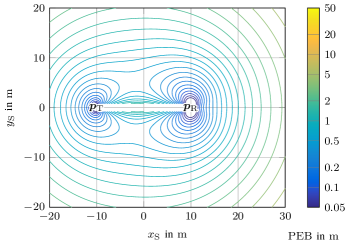
Figure 2: Logarithmic plot of the PEB for a varying $\bm{p}_{\mathrm{S}}$ with $P=2$ subcarriers and $N_{\mathrm{Tx}}=15$, $N_{\mathrm{Rx}}=3$.

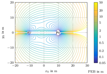
Figure 3: Logarithmic plot of the PEB for a varying $\bm{p}_{\mathrm{S}}$ with $P=1$ subcarrier and $N_{\mathrm{Tx}}=15$, $N_{\mathrm{Rx}}=3$.

Let us re-write (LABEL:equ:SPEBconstr) in terms of the EFIM by use of the properties of the Schur-complement:

$$\begin{split}&\operatorname{SPEB}=\operatorname{tr}((\bm{K}\bm{J}_{\mathrm{eh}}\bm{K}^{T})^{-1}),\\ &\bm{J}_{\mathrm{eh}}=\bm{J}_{22}-\bm{J}_{12}^{T}\bm{u}\left(\bm{u}^{T}\bm{J}_{11}\bm{u}\right)^{-1}\bm{u}^{T}\bm{J}_{12},\end{split}$$ (29)

$$\begin{split}&\bm{J}_{12}^{T}\bm{u}\left(\bm{u}^{T}\bm{J}_{11}\bm{u}\right)^{-1}\bm{u}^{T}\bm{J}_{12}\\ &=\frac{1}{j_{11}}\begin{bmatrix}j_{13}^{2}+j_{23}^{2}&j_{13}j_{14}+j_{23}j_{24}&0\\ j_{13}j_{14}+j_{23}j_{24}&j_{\mathrm{eh}}&0\\ 0&0&0\end{bmatrix},\end{split}$$ (30)

$$\frac{j_{\mathrm{eh}}}{j_{11}}=\frac{2}{\sigma_{\eta}^{2}}N_{\mathrm{R}}\lvert h_{1}\rvert^{2}\frac{\Bigl{(}\sum\limits_{p}\operatorname{Im}(\dot{\bm{a}}_{\mathrm{T},1}^{T}\bm{R}_{s}[p]\bm{a}_{\mathrm{T},1}^{\ast})\Bigr{)}^{2}}{\sum\limits_{p}\bm{a}_{\mathrm{T},1}^{T}\bm{R}_{s}[p]\bm{a}_{\mathrm{T},1}^{\ast}}.$$ (31)

Note that $j_{\mathrm{eh}}/j_{11}$ is the same as $(j_{14}^{2}+j_{24}^{2})/j_{11}$ in (16) with the corresponding real part squared removed from the absolute value squared in the numerator. As the constants in front of the fraction, as well as the numerator and the denominator are positive, the receiver can have more information about the AoD if the channel gain is known, but only if there is at least one $\operatorname{Re}(b_{p,21})\neq 0$. There is no change for the other parameters. Therefore, there is no benefit in knowing the channel gain if an optimal beamforming is used.

VI Numerical Results

VI-A Fixed Transmitter and Receiver Role

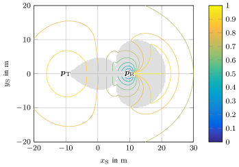
Figure 4: Share of $P_{\mathrm{T}}$ allocated onto $\bm{a}_{\mathrm{T},1}^{T}$, ($\sum_{p}b_{p,11}/P_{\mathrm{T}}$) for $N_{\mathrm{Tx}}=15$, $N_{\mathrm{Rx}}=3$. Rank-1 beamforming is optimal in the shaded area.

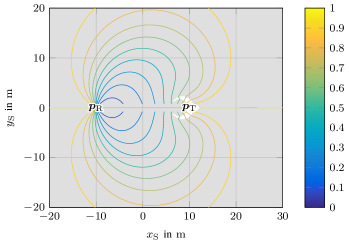
Figure 5: Share of $P_{\mathrm{T}}$ allocated onto $\bm{a}_{\mathrm{T},1}^{T}$, ($\sum_{p}b_{p,11}/P_{\mathrm{T}}$) for $N_{\mathrm{Tx}}=3$, $N_{\mathrm{Rx}}=15$. Rank-1 beamforming is optimal in the shaded area.

Consider a symmetric multicarrier system at $3.8\text{\,}\mathrm{GHz}$ center frequency with $P=2$ subcarriers under the narrowband assumption, $N_{\mathrm{T}}=15$, $N_{\mathrm{R}}=3$ and uniform circular arrays (UCAs) with $\lambda/2$ antenna spacing. Let $\bm{p}_{\mathrm{T}}^{T}=[-10,0]\,$\mathrm{m}$$, $\bm{p}_{\mathrm{R}}^{T}=[10,0]\,$\mathrm{m}$$, $\sigma_{\eta}^{2}=$2.4\text{\times}{10}^{-14}\text{\,}\mathrm{W}$$, $P_{\mathrm{T}}=$10\text{\,}\mathrm{mW}$$ and $\omega_{p}=2\pi p\cdot$2.4\text{\,}\mathrm{MHz}$$, which corresponds to a noise spectral density of $-170\text{\,}\mathrm{dBm}\mathrm{/}\mathrm{Hz}$. The CRB is independent of the phase of $h_{1}$ and its absolute value is modeled as

$$\lvert h_{1}\rvert=$0.1\text{\,}\mathrm{m}$\cdot\lambda/(4\pi d_{\mathrm{TS}}d_{\mathrm{SR}}).$$ (32)

The radar cross section (RCS) in (32) is constant: $$0.01\text{\,}\mathrm{m}^{2}$(4\pi)$. Note that the CRB is independent of whether the path-loss is taken into account here, because the RCS is assumed to be unknown. In Fig. 2, the position of the scatterer is varied, and the beamforming optimization is carried out for each grid point to obtain the position error bound ($\operatorname{PEB}=\sqrt{\operatorname{SPEB}}$). As expected, the $\operatorname{PEB}$ is smallest close to $\bm{p}_{\mathrm{T}}$ and $\bm{p}_{\mathrm{R}}$ and increases with increasing distance, or when the scatterer is close to the baseline of the radar, i.e. the line segment between $\bm{p}_{\mathrm{T}}$ and $\bm{p}_{\mathrm{R}}$ [16, Ch. 3], because the delay and the angles give little information in this area. There are two regions for the contour lines:

• For a larger $\operatorname{PEB}$, there is an oval corresponding to a large $d_{\mathrm{TS}}$ and $d_{\mathrm{SR}}$, and there are two contour lines close to the baseline, one on each side of it. The oval resembles the well-known Cassini oval.

• For a smaller $\operatorname{PEB}$, there are two contour lines, one around $\bm{p}_{\mathrm{T}}$ and one around $\bm{p}_{\mathrm{R}}$, similar to the Cassini ovals.

Let us compare this to a scenario inspired by [5], where we only have $P=1$ subcarrier, but the same transmit power, see Fig. 3. Unlike [5], we assume that the RCS is unknown, which requires rank-2 beamforming on the subcarrier to ensure that $\bm{K}\bm{J}_{\mathrm{e}}\bm{K}^{T}$ is full-rank, because delay estimation is impossible with $P=1$, whereas only rank-1 beamforming is used in [5]. The PEB obtained by optimization for $P=1$ is significantly larger than the PEB obtained with $P=2$ (Fig. 2), especially when the scatterer is further way from the baseline or when it is close to the half-lines that extend the baseline. Note that for $P=1$, it is impossible to estimate a $\bm{p}_{\mathrm{S}}$ that lies on the extended baseline, because the distance cannot be determined from the AoD and AoA due to the geometry. The significant performance difference between $P=1$ and $P=2$ shows that delay estimation is highly beneficial even at a small bandwidth ($\omega_{\pm 1}=\pm 2\pi\cdot$2.4\text{\,}\mathrm{MHz}$$).

Let us return to the scenario with $P=2$: Fig. 4 shows the share of transmit power allocated towards $\bm{a}_{\mathrm{T},1}^{T}$, i.e. $\sum_{p}b_{p,11}/P_{\mathrm{T}}$, which is between $8.8\text{\,}\mathrm{\char 37\relax}$ and $100\text{\,}\mathrm{\char 37\relax}$ in the area considered. It is small close to $\bm{p}_{\mathrm{R}}$, but increases significantly on the side of $\bm{p}_{\mathrm{R}}$ that faces away from $\bm{p}_{\mathrm{T}}$ at the same time. As $d_{\mathrm{TS}}$ and $d_{\mathrm{SR}}$ increase, the information that the AoD and AoA give decreases, while that of the delay is independent of $d_{\mathrm{TS}}$ and $d_{\mathrm{SR}}$, see (9). Due to this, more power is allocated towards $\dot{\bm{a}}_{\mathrm{T},1}^{T}$ to compensate for the loss in AoD accuracy here, because $N_{\mathrm{Tx}}>N_{\mathrm{Rx}}$. Fig. 4 also shows when rank-1 beamforming is an optimal solution and when the full-rank solution is optimal. For $N_{\mathrm{Rx}}\geq 2$, there are areas where rank-1 beamforming is optimal and areas where full-rank beamforming is optimal. The former is optimal, when the scatterer is close to the baseline or close to the receiver. In that part of the area close to $\bm{p}_{\mathrm{T}}$ where rank-1 beamforming is optimal, there is no benefit of a second beam, because delay estimation gives little information close to the baseline. In the corresponding part close to $\bm{p}_{\mathrm{R}}$, there is no benefit of a second beam, because the performance of AoA estimation is good, and AoD / delay estimation performs well. There is small notch between the two areas just discussed, where an additional beam that enables AoD and delay estimation is beneficial, because a large share of power is dedicated to AoD estimation, which reduces the information from AoA estimation, and delay estimation does not give much information, since the scatterer is close to the baseline.

Note that regardless of whether rank-1 or full rank beamforming are optimal, the optimal beams typically are weighted between $\bm{a}_{\mathrm{T},1}^{T}$ and $\dot{\bm{a}}_{\mathrm{T},1}^{T}$, i.e. $\operatorname{Im}(b_{p,21})\neq 0$.

Consider also the power allocation and optimal strategy for the switched roles, i.e. $N_{\mathrm{Tx}}=3$, $N_{\mathrm{Rx}}=15$, see Fig. 5. Due to the larger number of receive antennas, rank-1 beamforming is optimal almost everywhere. Similarly to Fig. 4, the share of power towards $\bm{a}_{\mathrm{T},1}^{T}$ is small close to $\bm{p}_{\mathrm{R}}$, but increases significantly on the side of $\bm{p}_{\mathrm{R}}$ that faces away from $\bm{p}_{\mathrm{T}}$ at the same time. But contrary to Fig. 4, the share of power allocated into $\dot{\bm{a}}_{\mathrm{T},1}^{T}$ decreases as $d_{\mathrm{TS}}$ and $d_{\mathrm{SR}}$ increase, because $N_{\mathrm{Rx}}>N_{\mathrm{Tx}}$ here.

VI-B Switchable Transmitter and Receiver Role

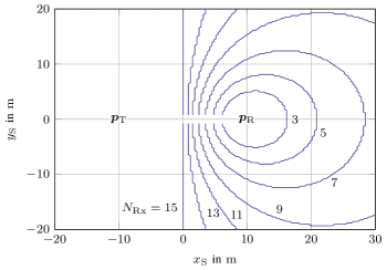
Figure 6: Switchable roles for a varying $N_{\mathrm{Rx}}$: For a scatterer outside of the contour line, it is better to switch roles.

There is an additional degree of freedom in a bistatic radar system when both ends can transmit and receive: one can select which transmit/receive point (TRP) of the radar transmits and which receives. Fig. 6 shows which TRP should transmit or receive based on the setup in Sect. VI-A. In addition, $N_{\mathrm{Rx}}$ is varied from $3$ to $15$. Firstly, consider the case, where both TRPs are set up symmetrically, i.e. they have the same antenna arrays and symmetric orientation. In this case, the optimization result is that the TRP that is closer to the scatterer should always receive. Only when $d_{\mathrm{TS}}=d_{\mathrm{SR}}$, the performance in both directions is the same, and time-sharing between them is also an optimal solution.

Secondly, consider $N_{\mathrm{Rx}}\neq 15$. Fig. 6 shows that as in the symmetric setup, it is optimal that exactly one TRP transmits. The contour lines correspond to those scatterer positions with the same performance in both directions is the same, where time-sharing is also an optimal solution. As $N_{\mathrm{Rx}}$ increases, the area where the role of the TRPs shown in the figure is optimal increases. Note that once it is known which TRP transmits, the optimal beamforming is the same as discussed in the previous subsection.

VII Conclusion

In this paper, the optimal beamforming for bistatic sensing, which could be part of a JC&S system, was discussed and it was shown numerically that a rank-1 solution is optimal for some parameters, and a full-rank solution is optimal others, which is not considered by many papers in the literature. It was further shown that using more than one subcarrier is highly beneficial, because it enables delay estimation. Numerical results with the additional degree of freedom that both ends of the bistatic radar can transmit and receive show that it is optimal when exactly one TRP transmits, and one receives, while selecting which TRP should transmit and which receive varies with the number of antennas and the target’s position.

[Intermediate Results Needed to Compute the FIM] The derivatives of $\bm{m}[p]$ w.r.t. the parameters included the in the parameter vector $\bm{\phi}$ are given by

$$\frac{\partial\bm{m}[p]}{\partial\bm{h}_{1,\mathrm{R}}} =\bm{a}_{\mathrm{R},1}[p]\bm{a}_{\mathrm{T},l}^{T}[p]e^{-j\omega_{p}\tau_{1}}\bm{s}[p],$$ (33)

$$\frac{\partial\bm{m}[p]}{\partial\bm{h}_{1,\mathrm{I}}} =j\frac{\partial m[p]}{\partial\bm{h}_{1,\mathrm{R}}},$$ (34)

$$\frac{\partial\bm{m}[p]}{\partial\tau_{1}} =-j\omega_{p}h_{1}\bm{a}_{\mathrm{R},1}[p]\bm{a}_{\mathrm{T},1}^{T}[p]e^{-j\omega_{p}\tau_{1}}\bm{s}[p],$$ (35)

$$\frac{\partial\bm{m}[p]}{\partial\tilde{\theta}_{\mathrm{T},1}} =h_{1}\bm{a}_{\mathrm{R},1}[p]\dot{\bm{a}}_{\mathrm{T},1}^{T}[p]e^{-j\omega_{p}\tau_{1}}\bm{s}[p],$$ (36)

$$\frac{\partial\bm{m}[p]}{\partial\tilde{\theta}_{\mathrm{R},1}} =h_{1}\dot{\bm{a}}_{\mathrm{R},1}[p]\bm{a}_{\mathrm{T},1}^{T}[p]e^{-j\omega_{p}\tau_{1}}\bm{s}[p].$$ (37)

$\bm{J}_{11}$ and $\bm{J}_{12}$ are given by

$$\bm{J}_{11} =\operatorname{diag}(j_{11},j_{22}),$$ (38)

$$j_{11} =j_{22}=\frac{2}{\sigma_{\eta}^{2}}N_{\mathrm{R}}\sum\limits_{p}\bm{a}_{\mathrm{T},1}^{T}[p]\bm{R}_{s}[p]\bm{a}_{\mathrm{T},1}^{\ast}[p],$$ (39)

$$\bm{J}_{12} =\begin{bmatrix}j_{13}&j_{14}&0\\ j_{23}&j_{24}&0\end{bmatrix},$$ (40)

$$j_{13} =\frac{2}{\sigma_{\eta}^{2}}N_{\mathrm{R}}h_{1,\mathrm{I}}\sum\limits_{p}\omega_{p}\bm{a}_{\mathrm{T},1}^{T}[p]\bm{R}_{s}[p]\bm{a}_{\mathrm{T},1}^{\ast}[p],$$ (41)

$$j_{23} =-\frac{\mathstrut 2}{\sigma_{\eta}^{2}}N_{\mathrm{R}}h_{1,\mathrm{R}}\sum\limits_{p}\omega_{p}\bm{a}_{\mathrm{T},1}^{T}[p]\bm{R}_{s}[p]\bm{a}_{\mathrm{T},1}^{\ast}[p],$$ (42)

$$j_{14} =\frac{2}{\sigma_{\eta}^{2}}N_{\mathrm{R}}\sum\limits_{p}\operatorname{Re}(h_{1}\dot{\bm{a}}_{\mathrm{T},1}^{T}[p]\bm{R}_{s}[p]\bm{a}_{\mathrm{T},1}^{\ast}[p]),$$ (43)

$$j_{24} =\frac{2}{\sigma_{\eta}^{2}}N_{\mathrm{R}}\sum\limits_{p}\operatorname{Im}(h_{1}\dot{\bm{a}}_{\mathrm{T},1}^{T}[p]\bm{R}_{s}[p]\bm{a}_{\mathrm{T},1}^{\ast}[p]).$$ (44)

References

- [1] M. S. Greco, P. Stinco, F. Gini, and A. Farina, “Cramér-Rao bounds and selection of bistatic channels for multistatic radar systems,” IEEE Trans. Aerosp. Electron. Syst., vol. 47, no. 4, pp. 2934–2948, Oct. 2011, doi: 10.1109/TAES.2011.6034675.
- [2] S. Gogineni, M. Rangaswamy, B. D. Rigling, and A. Nehorai, “Cramér-Rao bounds for UMTS-based passive multistatic radar,” IEEE Trans. Signal Process., vol. 62, no. 1, pp. 95–106, Jan. 2014, doi: 10.1109/TSP.2013.2284758.
- [3] Q. He, J. Hu, R. S. Blum, and Y. Wu, “Generalized Cramér–Rao bound for joint estimation of target position and velocity for active and passive radar networks,” IEEE Trans. Signal Process., vol. 64, no. 8, pp. 2078–2089, Apr. 2016, doi: 10.1109/TSP.2015.2510978.
- [4] J. Tong, H. Gaoming, T. Wei, and P. Huafu, “Cramér-Rao lower bound analysis for stochastic model based target parameter estimation in multistatic passive radar with direct-path interference,” IEEE Access, vol. 7, pp. 106 761–106 772, 2019, doi: 10.1109/ACCESS.2019.2926353.
- [5] F. Zabini, E. Paolini, W. Xu, and A. Giorgetti, “Joint sensing and communication with multiple antennas and bistatic configuration,” in Proc. IEEE Int. Conf. Commun. Workshops (ICC Workshops), Rome, Italy, May/Jun. 2023, pp. 1416–1421, doi: 10.1109/ICCWORKSHOPS57953.2023.10283688.
- [6] A. Kakkavas, M. H. Castañeda García, R. A. Stirling-Gallacher, and J. A. Nossek, “Performance limits of single-anchor millimeter-wave positioning,” IEEE Trans. Wireless Commun., vol. 18, no. 11, pp. 5196–5210, Nov. 2019, doi: 10.1109/TWC.2019.2934460.
- [7] B. Friedlander, “Wireless direction-finding fundamentals,” in Classical and Modern Direction-of-Arrival Estimation, T. E. Tuncer and B. Friedlander, Eds. Burlington, MA, USA: Academic Press, 2009, pp. 1–51, doi: 10.1016/B978-0-12-374524-8.00001-5.
- [8] S. M. Kay, Fundamentals of Statistical Signal Processing: Estimation Theory, ser. Prentice-Hall Signal Processing Series. Upper Saddle River, NJ, USA: Prentice Hall PTR, 1993, vol. 1.
- [9] Y. Shen and M. Z. Win, “Fundamental limits of wideband localization—Part I: A general framework,” IEEE Trans. Inf. Theory, vol. 56, no. 10, pp. 4956–4980, Oct. 2010, doi: 10.1109/TIT.2010.2060110.
- [10] K. Nordström, “Convexity of the inverse and Moore-Penrose inverse,” Linear Algebra Applicat., vol. 434, no. 6, pp. 1489–1512, Mar. 2011, doi: 10.1016/j.laa.2010.11.023.
- [11] R. Hunger, Analysis and Transceiver Design for the MIMO Broadcast Channel, ser. Foundations in Signal Processing, Communications and Networking. Berlin, Heidelberg: Springer, 2013, no. 8.
- [12] W. Xu, A. Dammann, and T. Laas, “Where are the things of the internet? Precise time of arrival estimation for IoT positioning,” in The Fifth Generation (5G) of Wireless Communication, A. Kishk, Ed. IntechOpen, Nov. 2018, pp. 59–79, doi: 10.5772/intechopen.78063.
- [13] S. M. Sherman and D. K. Barton, Monopulse Principles and Techniques, 2nd ed. Boston, MA, USA: Artech House, 2011.
- [14] Y. Xiong, F. Liu, Y. Cui, W. Yuan, T. X. Han, and G. Caire, “On the fundamental tradeoff of integrated sensing and communications under Gaussian channels,” IEEE Trans. Inf. Theory, vol. 69, no. 9, pp. 5723–5751, Sep. 2023, doi: 10.1109/TIT.2023.3284449.
- [15] P. Stoica and B. C. Ng, “On the Cramér–Rao bound under parametric constraints,” IEEE Signal Process. Lett., vol. 5, no. 7, pp. 177–179, Jul. 1998, doi: 10.1109/97.700921.
- [16] N. J. Willis, Bistatic Radar, 2nd ed. Raleigh, NC, USA: SciTech, 2005.