Stochastic Geometry Analysis of EMF Exposure of Idle Users and Network Performance with Dynamic Beamforming

Abstract

This paper presents a novel mathematical framework based on stochastic geometry to investigate the electromagnetic field exposure of idle and active users in cellular networks implementing dynamic beamforming. Accurate modeling of antenna gain becomes crucial in this context, encompassing both the main and the side lobes. The marginal distribution of EMF exposure for each type of users is initially derived. Subsequently, network performance is scrutinized by introducing a new metric aimed at ensuring minimal downlink coverage while simultaneously maintaining EMF exposure below distinct thresholds for both idle and active users. The metrics exhibit a high dependency on various parameters, such as the distance between active and idle users and the number of antenna elements.

I Introduction

The rapid evolution of wireless communication technologies has sparked growing concerns about the potential risks associated with electromagnetic field (EMF) exposure stemming from wireless network infrastructures. Among the effects associated with non-ionizing frequencies, thermal effects stand out as the sole impact unanimously acknowledged within the scientific community [1]. Entities such as the International Commission on Non-Ionizing Radiation Protection (ICNIRP) establish maximal EMF exposure thresholds based on conservative margins and literature review, specifying basic restrictions in terms of specific absorption rate (SAR) or incident power density (IPD) [2]. Nations or regional entities can then adopt these guidelines or enact more stringent legislation.

A noteworthy innovation introduced by the 5th generation of cellular networks and subsequent generations is dynamic beamforming (DBF). Using multiple antennas at the base station (BS), DBF enables the formation of narrow beams to mitigate interference. While this significantly enhances the signal-to-interference-plus-noise ratio (SINR), it results in higher EMF exposure for active users (AUs) calling for the beam, compared to idle users (IUs) who are not active in the network and who experience lower EMF exposure on average with shorter exposure times [3]. The distinction in exposure between AUs and IUs can be leveraged to establish different exposure constraints for AUs and IUs. This is in line with the desire to establish safe zones called ”reduced EMF exposure areas” for IUs in facilities such as hospitals, schools, or public buildings such as train stations [4]. In this context, investigating the exposure to EMF experienced by IUs becomes crucial, especially to understand how it varies based on the distance from an AU [5]. The IU’s EMF exposure is a sum of the EMF exposure caused by the BS serving the AU and that caused by interfering BSs. Notably, the shape of the beam plays a pivotal role in influencing IU’s EMF exposure.

The EMF exposure for IUs is intricately linked to the minimal SINR required and the maximum permitted EMF exposure for AUs, dictating how network operators design their networks. To provide a comprehensive analysis, this paper delves into a study of global network performance by simultaneously examining the exposure and coverage for AUs, in addition to the EMF exposure experienced by IUs.

The metrics for such an analysis involve random parameters, including network topology, BS beam directions, and propagation channel. To capture this inherent randomness, stochastic geometry (SG) emerges as an efficient tool. Within this framework, BSs are modeled as point processes (PPs), allowing the formulation of network performance in integrals that are both mathematically and computationally tractable.

Motivated by these considerations, the primary aim of this paper is to introduce a comprehensive mathematical framework for studying network performance in terms of EMF exposure for AUs and IUs, as well as the coverage of AUs, employing an antenna gain model that closely approximates real-world conditions.

I-A Related Works

5G and beyond: exploring EMF exposure

Numerous studies have tried to evaluate and forecast EMF exposure in 5G and beyond 5G networks. Compared to EMF exposure assessment in older network generations, the examination of EMF exposure in a 5G network introduces heightened complexity due to the coexistence of heterogeneous networks incorporating macro, small, and femto cells. This complexity is further compounded by the utilization of higher frequencies and the integration of active antennas. The global EMF exposure is encapsulated by the exposure index (EI) [6], encompassing both uplink (UL) and downlink (DL) EMF exposure. Studies on EMF exposure in the context of 5G can be broadly categorized into two main approaches: those based on simulation models and those based on field measurements. Notably, in the 5G context, a specific measurement protocol for the DL has been defined, implemented, and validated in urban environments [5] and [7]. This protocol calculates the time-averaged instantaneous exposure and maximum exposure for 5G base stations, enabling the assessment of EMF exposure during both user calls and idle states.

The French spectrum regulator ANFR, has contributed to this area by conducting a study [8] comparing EMF levels before and after the installation of 5G equipment. Their findings indicated that radiation levels remained similar. Another study by ANFR [3], utilizing simulations, demonstrated higher EMF exposure for AUs and lower exposure for IUs in a 5G network compared to previous generations. Additionally, algorithmic investigations in [9] affirmed that narrower beams result in lower EMF exposure. Comprehensive reviews on the current state of EMF exposure evaluation for 5G base stations are available in [10] and [11], highlighting the reduction in EMF exposure levels with the implementation of DBF.

Various strategies have been proposed to further mitigate EMF exposure levels. For instance, an optimization algorithm introduced in [12] aims to minimize UL and DL EMF exposure while maintaining quality of service using a small cell network in conjunction with a macro cell network. In another approach [13], a novel simulation method employs a smart power control scheme to minimize the EI. Recent advancements explore the utilization of reconfigurable intelligent surfaces (RIS) in beyond 5G networks, creating zones with reduced EMF exposure while maintaining high data rates. The efficacy of this method has been substantiated through ray-tracing simulations [14, 15], as well as algorithmic optimization of RIS phases [16].

Nevertheless, challenges persist; in-situ measurements offer insights into EMF exposure at limited locations under specific conditions, while deterministic numerical evaluations struggle to capture all sources of randomness within the network efficiently and within a reasonable time.

Dynamic beamforming models in stochastic geometry

SG emerges as a potent tool for computing performance metrics in large networks characterized by various random parameters. In this context, BSs are frequently modeled as homogeneous Poisson point processes (PPPs), striking a balance between accuracy and computational tractability. SG has been extensively used to focus on aspects such as SINR and ergodic data rate [17, 18]. Numerous features have been intensively studied, including DBF.

Models of antenna patterns are derived to approach the theoretical distribution of the antenna factor of a Uniform Linear Array (ULA), which is inherently intractable [19, 20]. The sectored antenna pattern, or flat-top pattern, represents the most widely used model. Although this model introduces huge discrepancies when calculating performance metrics, it preserves mathematical tractability by assuming a flat gain for the main lobes and a lower gain for the side lobes. It has been applied to study SINR in multi-tier millimeter-wave (mmWave) cellular networks with beamsteering errors [21] and the impact of beam misalignment due to mobility and handovers [22]. The flat-top pattern has found utility in diverse scenarios, including the study of SINR and Conditional Success Transmission Probability (STP) in downlink non-orthogonal multiple access networks [23] and in mmWave heterogeneous networks considering temporal traffic arrivals [24]. In ultra-dense networks, the antenna pattern is sometimes modeled as a 3D flat-top pattern, as evidenced in studies on mmWave networks [25] and terahertz networks [26].

A notable alternative to the flat-top pattern is the cosine approximation of the main lobe of the theoretical ULA pattern, introduced in [20]. This cosine model yields a complementary cumulative distribution function (CCDF) of SINR closer to the one obtained through Monte Carlo simulations based on the theoretical pattern than the one obtained using the flat-top pattern. The cosine model has been applied in various contexts, such as Poisson cluster processes [27] and joint radar communication systems [28].

A Gaussian approximation of the main beam, introduced in [29], has been employed to study the ergodic capacity in mmWave networks with imperfect beam alignment. In comparison to the cosine model, which assumes null gain for the side lobes, the Gaussian model allows for the modeling of side lobes with a constant gain. This advantage proves beneficial for realistic studies on beam misalignment, as demonstrated in [30], where each BS is equipped with three ULAs oriented at 120^∘ intervals, in line with 3GPP specifications.

Finally, an unconventional approach employs a cylindrical array instead of the common ULA to study interference, as presented in [31]. This array is then modeled as a uniform circular array for the elevation angle and a vertical ULA for the azimuth angle, although the model lacks tractability and remains largely theoretical at present.

EMF exposure assessment using stochastic geometry

In recent years, SG has been instrumental in assessing IPD with the objective of optimizing it in Wireless Power Transfer (WPT) systems or minimizing it for EMF-aware applications. The flat-top model finds widespread application in WPT systems for energy harvesting [32, 33] and for analyzing energy correlation [34]. It has been utilized in works such as [35, 36], where the flat-top model is employed to estimate simultaneous wireless information and power transfer by computing a joint CCDF to strike a balance between coverage and harvested power. Additionally, the Gaussian model is used in [37] to explore the impact of imperfect beam alignment in mmWave WPT systems.

The initial works assessing EMF exposure within the SG framework are presented in [38], where authors utilize an empirical propagation model for a 5G network in mmWave scenarios, and in [39], where the theoretical distribution of EMF exposure is compared with an experimental distribution obtained from measurements in an urban environment. In [40], EMF exposure is analyzed while considering max-min fairness power control. The flat-top pattern is employed for EMF exposure analysis in sub-6 GHz and mmWave coexisting networks [41], and in [42], it is used for a joint analysis of EMF exposure and SINR in $\beta$-Ginibre PP and inhomogeneous Poisson PPs. Notably, these two works are the soles that incorporate DBF into the SG model for EMF exposure. Joint analyses of EMF exposure and SINR are also conducted in [43] for Manhattan networks, in [44] for user-centric cell-free networks, and in [45] for both UL and DL. An evaluation of EMF exposure caused by a user’s smartphone using SG is presented in [46], where the authors independently study the impact of network parameters on EMF exposure and signal-to-noise ratio.

However, a notable gap exists in the literature concerning the study of EMF exposure experienced by an IU in a DBF network, particularly within the SG framework. Additionally, the current models of antenna patterns struggle to accurately capture the characteristics of side lobes, thereby impacting certain network performance metrics. A preliminary work using the multi-cosine gain pattern is done in [47] for the case of a passive user (PU) in the network, indicating a user not calling a beam and for which no information is known about a possible proximity to an AU.

I-B Contributions

This paper addresses gaps in the literature by focusing on the evaluation of EMF exposure for IUs in the SG framework. It introduces a multi-cosine antenna gain model, which provides a more accurate representation by accounting for side lobes. The key contributions of this paper are outlined below:

1. EMF exposure of idle users: The paper introduces mathematical expressions that delineate the EMF exposure experienced AUs and IUs within the network. These mathematical expressions are calculated for several gain models and compared to the introduced multi-cosine pattern. Specifically, the paper provides:

   1. Mean and variance for IU EMF exposure;

   2. Marginal cumulative distribution function (CDF) characterizing any user’s EMF exposure for several gain models.

2. Spatial performance metrics: The study extends beyond EMF exposure, encompassing a broader analysis of network performance. This is achieved by jointly computing a spatial CDF that considers (1) SINR for an AU, (2) EMF exposure for an AU and (3) EMF exposure for an IU.

These metrics are investigated as functions of the distance between the AU and the IU, as well as functions of the number of antennas at the BS, providing a comprehensive understanding of the network’s performance dynamics.

II System Model

II-A Topology

Let the two-dimensional spatial domain $\mathcal{B}\in\mathbb{R}^{2}$ be the network area, defined as a disk with a radius $\tau$ and centered at the origin. Within $\mathcal{B}$, let $\Psi={X_{i}}$ denote the PPP representing the locations of BS $X_{i}$, all sharing the same technology, belonging to the same network provider, operating at a carrier frequency $f$, and being able to transmit at a maximum power $P_{t}$. The density of BSs in $\Psi$ is denoted by $\lambda$. Each BS is situated at a height $z>0$ relative to the users. The AU is positioned at the origin and is served by the nearest BS, while all other BSs act as potential interferers. An IU is located at a distance $d$ from the AU and form a random angle $\theta$ with the serving BS, as can be seen from Fig. 1. The distance between the AU and $X_{i}$ is denoted $R_{i}$, the angle formed between the IU and $X_{i}$ is denoted $\Theta_{i}$ and the distance between the IU and $X_{i}$ is denoted $P_{i}=\sqrt{R_{i}^{2}+d^{2}-2R_{i}d\cos(\Theta_{i})}$. Additionally, an angle $\delta_{i}=\operatorname{sign}(\Theta_{i})\arccos\left((R_{i}-d\cos\Theta_{i})/P_{i}\right)$ is employed to describe the angle between the AU and the IU from the perspective of $X_{i}$. The boresight direction of $X_{i}$ forms an angle $\xi_{i}$ with the AU. The serving BS and the associated distances and angles are indexed as $0$, with the boresight of $X_{0}$ directed towards the AU (i.e., $\theta_{0}=0$).

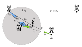
Figure 1: Active and idle user

In this configuration, the equipment of the AU is considered with a unitary and isotropic gain. Each BS is equipped with three identical ULAs oriented at 120^∘ intervals, following 3GPP specifications, with each array containing $N$ antennas with half-wavelength spacing. Consequently, the angle $\xi_{i}$ is a random variable in the interval $[0,2\pi/3[$. Intra-cell interference is neglected for simplicity, and an exclusion radius $r_{e}$ around the user ensures no BS is located within this region. The normalized gain $G(\xi)$ is uniformly scaled by the maximum gain $G_{\textrm{max}}=N$, and defined in Subsection II-C. For a conservative approach, the network is considered fully loaded, with each ULA communicating with one user.

For a PPP, the probability density function (PDF) of $R_{0}$ is given by

$$f_{R_{0}}(r)=\frac{2\pi\lambda r\exp(-\lambda\pi r^{2})}{F_{R_{0}}(r_{e})-F_{R_{0}}(\tau)}$$ (1)

where $F_{R_{0}}(r)=\exp(-\lambda\pi r^{2})$.

It is essential to note that for the impact of $d$ to be meaningful, the IU must be in the same cell as the AU. Subsequent analyses will, therefore, operate under the assumption that $d$ is smaller than the mean cell radius, defined as $(2\sqrt{\lambda})^{-1}$. In instances where the distance exceeds this threshold, the user will be categorized as a PU, indicating no correlation with the location of the AU, for which expressions are derived in [47]. It is also assumed that $\tau>>d$.

II-B Propagation Model

The propagation model is defined as

$$P_{r,i}=P_{t}G_{i}|h_{i}|^{2}l_{i}$$ (2)

where $P_{r,i}$ is the received power from BS $X_{i}$, $G_{i}$ is the BS gain towards the user, $|h_{i}|^{2}$ accounts for the fading and $l_{i}$ is the path loss attenuation. Specifically, $l_{i}=l(X_{i})=\kappa^{-1}\left(R_{i}^{2}+z^{2}\right)^{-\alpha/2}$ for a distance $R_{i}$ between $X_{i}$ and the AU, with $\alpha>2$ the path loss exponent and $\kappa=(4\pi f/c_{0})^{2}$ where $c_{0}$ is the speed of light. For the path between $X_{i}$ and the IU, $\tilde{l}(X_{i})=\kappa^{-1}\left(P_{i}^{2}+z^{2}\right)^{-\alpha/2}$. The channel $h_{i}$ follows a Nakagami-$m$ fading model, making $|h_{i}|^{2}$ gamma-distributed with shape parameter $m$ and scale parameter $1/m$. Consequently, the CDF of $|h_{i}|^{2}$ is expressed as $F_{|h|^{2}}(x)=\gamma(m,mx)/\Gamma(m)$.

Define $\bar{P}_{r,i}\!=\!\bar{P}_{r}(r_{i})\!=\!P_{t}l_{i}(r_{i})$. Let $S_{0}(0)\!=\!\bar{P}_{r}(r_{0})|h_{0}|^{2}$ be the useful power received by the AU from $X_{0}$ and let $I_{0}(0)=\sum_{i\in\Psi\setminus\left\{X_{0}\right\}}\bar{P}_{r,i}(r_{i})G_{i}(\xi)|h_{i}|^{2}$ be the aggregate interference at the AU’s location. Similarly, the signal coming from $X_{0}$ and reaching the IU is $S_{0}(d)\!=\!\bar{P}_{r}(p_{0})G(\delta_{0})|h_{0}|^{2}$ and the aggregate interference at the IU’s location is $I_{0}(d)=\sum_{i\in\Psi\setminus\left\{X_{0}\right\}}\bar{P}_{r,i}(p_{i})G_{i}(\xi+\delta_{i})|h_{i}|^{2}$. Based on these definitions, the SINR experienced by the AU and conditioned on the distance to the serving BS is given by

$$\text{{SINR}}_{0}=\frac{S_{0}}{I_{0}+\sigma^{2}}$$ (3)

where $\sigma^{2}=k\,B\,T\,\mathcal{F}$ is the thermal noise power, with $k$ the Boltzmann constant, $B$ the bandwidth, $T$ the temperature and $\mathcal{F}$ the noise figure. In the following, the performance metrics will be derived for the user DL power exposure defined as

$$\mathcal{P}=\sum_{i\in\Psi}\bar{P}_{r,i}\,G_{i}\,|h_{i}|^{2}=S_{0}+I_{0},$$ (4)

which can be converted into a total IPD as

$$\mathcal{S}=\sum_{i\in\Psi}\frac{P_{t}\,G_{i}\,|h_{i}|^{2}}{4\pi\left(r_{i}^{2}+z^{2}\right)^{\alpha/2}}=\frac{\kappa}{4\pi}\mathcal{P}$$ (5)

by definition.

II-C Antenna Pattern Models

The normalized gain of one ULA with $N$ omnidirectional antenna elements and half-wavelength spacing is given by

$$G_{act}(\varphi)=\frac{\sin^{2}\left(\frac{\pi\,N}{2}\,\sin(\varphi)\right)}{N^{2}\,\sin^{2}\left(\frac{\pi}{2}\,\sin(\varphi)\right)}$$ (6)

where $\varphi\in[-\pi/3,\pi/3[$ and $\varphi=0$ corresponds to the maximal gain of the main lobe $G_{act}(0)=1$. While the gain function is closely approximated by a squared cardinal sinus function, this approximation also yields intractable mathematical expressions for calculating performance metrics. Instead, the flat-top antenna pattern is widely used in the literature, and given by

$$G_{ft}(\varphi)=\left\{\begin{array}[]{ll}1&\text{if }|\varphi|\leq\varphi_{3\text{dB}}\\ g&\text{otherwise}\end{array}\right.$$ (7)

where $\varphi_{3\text{dB}}$ is half of the half-power beamwidth (HPBW) of the actual pattern and $g$ is the side lobes gain chosen.

The cosine antenna pattern [20] approximates the main lobe of the actual pattern while assuming null gain for the side loves and is expressed as

$$G_{cos}(\varphi)=\left\{\begin{array}[]{ll}\cos^{2}\left(N\pi\varphi/4\right)&\text{if }|\varphi|\leq 2/N\\ 0&\text{otherwise.}\end{array}\right.$$ (8)

The gaussian approximation is given by

$$G_{G}(\varphi)=(N-g)\exp(-\eta\varphi^{2})+g$$ (9)

where $\varphi\in[-\pi/3,\pi/3[$ and $\eta=\ln\left(\frac{N-g}{N/2-g}\right)/\varphi_{3\text{dB}}^{2}$.

Lastly, we introduce the multi-cosine antenna pattern defined as

$$G_{mc}(\varphi)=\left\{\begin{array}[]{ll}\!\cos^{2}\!\left(\frac{N\pi\varphi}{4}\right)\!&\text{if }|\varphi|\leq 2/N\\ \!\chi_{k}\sin^{2}\!\left(\frac{N\pi\varphi}{2}\right)\!&\text{if }\frac{2k}{N}\!\leq\!|\varphi|\!\leq\!\frac{2k+2}{N}\end{array}\right.$$ (10)

where $\chi_{k}=\frac{\sin^{2}(Nx_{k})}{N^{2}\sin^{2}(x_{k})}$ is the extrema of the $k$th side lobe of the theoretical gain function, with $0\leq k\leq k_{\textrm{max}}$ and $\chi_{0}\!=\!1$. The choice of $k_{\textrm{max}}$ is flexible but should remain below $\left\lfloor N\sqrt{3}/4-1\right\rfloor$ to prevent side lobes from extending beyond each ULA’s sector. The values of $x_{k}$ are well approached by the ordered positive solutions of $N\tan(x)=\tan(Nx)$.

III Mathematical Framework

This section is organized as follows: Subsection III-A introduces the side calculations needed in the following subsections. […]

III-A Preliminaries

In this subsection, we initiate the analysis by computing the central moments of the approximate gain functions associated with each BS. Each BS is equipped with three identical ULAs, each designed to cover 120^∘. To mitigate intracell interference, it is assumed that the main beams of two distinct ULAs, employing the same carrier frequency simultaneously, cannot be in close proximity. Consequently, we make the assumption that the integral of the gain function over 360^∘ can be approximated by three times the integral of the gain function over 120^∘.

Proposition 1.

The $k$th moments ($k>0$) of the approximate gain functions are given by

$$\mathbb{E}\left[G_{ft}^{k}(\varphi)\right]=\frac{3}{\pi}\varphi_{3\textrm{dB}}(1-g^{k})+g^{k};$$ (11)

$$\mathbb{E}\left[G_{cos}^{k}(\varphi)\right]=\dfrac{6\,\Gamma(k+1/2)}{N{\pi}^{3/2}\Gamma(k+1)};$$ (12)

$$\mathbb{E}\left[G_{G}^{k}(\varphi)\right]=g^{k}+\frac{3}{2}\sum\limits_{p=1}^{k}\binom{k}{p}(N-g)^{p}g^{k-p}\frac{\operatorname{erf}\left(\tfrac{\pi\sqrt{p\eta}}{3}\right)}{\sqrt{\pi p\eta}};$$ (13)

$$\mathbb{E}\left[G_{mc}^{k}(\varphi)\right]=\dfrac{6\,\Gamma(k+1/2)}{N{\pi}^{3/2}\Gamma(k+1)}(1+\chi_{i_{\textrm{max}}}^{\dagger})$$ (14)

where $\operatorname{erf}(\cdot)$ is the error function and $\chi_{i_{\textrm{max}}}^{\dagger}=\sum\limits_{i=1}^{i_{\textrm{max}}}\chi_{i}$.

Proof.

The proof is obtained by integrating $\frac{3}{2\pi}\int_{-\pi/3}^{\pi/3}\!G^{2}(\varphi)d\varphi$. ∎

To derive metrics, whether the coverage of the EMF exposure, the characteristic function (CF) of the useful signal and interference must be calculated at the AU’s and the IU’s location. The CF of the useful signal is given in Proposition 2.

Proposition 2.

The CF of the useful signal for the propagation model in (2), from the point of view of the active user, conditioned on the distance to the nearest BS $R_{0}$, is

$$\phi_{S}(q;0|R_{0})=\mathbb{E}_{S_{0}}\left[e^{jq{S_{0}(R_{0})}}\right]=\left(1-jq\bar{P}_{r}(R_{0})/m\right)^{-m}.$$ (15)

From the point of view of the idle user, it is given by

$$\begin{split}\phi_{S}(q;d|X_{0})=\left(1-jq\bar{P}_{r}(P_{0})G(\delta_{0})/m\right)^{-m}\mathds{1}\left[|\delta_{0}|\leq\pi/3\right]\\ +\eta_{S}(q|X_{0})(1-\mathds{1}\left[|\delta_{0}|\leq\pi/3\right]).\end{split}$$ (16)

where $\eta_{S}(q|X_{0})$ depends on the considered gain pattern:

• Flat-top pattern

$$\begin{split}\eta_{S}(q|X_{0})=\frac{3\varphi_{3\textrm{dB}}}{\pi}\left(1-jq\bar{P}_{r}(P_{0})/m\right)^{-m}\\ +\left(1-\frac{3\varphi_{3\textrm{dB}}}{\pi}\right)\left(1-jq\bar{P}_{r}(P_{0})g/m\right)^{-m}\end{split}$$ (17)

• Gaussian pattern

$$\begin{split}&\eta_{S}(q|X_{0})=\left(1-jq\bar{P}_{r}(P_{0})g/m\right)^{-m}\\ &+\sum\limits_{p=1}^{\infty}\frac{3\operatorname{erf}\left(\tfrac{\pi\sqrt{p\eta}}{3}\right)}{2\sqrt{\pi p\eta}}(N-g)^{p}\frac{\left(jq\bar{P}_{r}(P_{0})\right)^{p}}{\left(1-\frac{jq\bar{P}_{r}(P_{0})}{m}\right)^{(m+p)}}\frac{\Gamma(m+p)}{\Gamma(m)m^{p}p!}\end{split}$$ (18)

• Multi-cos pattern

$$\eta_{S}(q|X_{0})=1+\frac{6(1+\chi_{i_{\textrm{max}}}^{\dagger})}{N\pi}\left(\!{}_{2}F_{1}\left(\frac{1}{2},m;1;\frac{jq\bar{P}_{r}(P_{0})}{m}\right)-1\right)$$ (19)

Proof.

The proof of (15) is straightforward after applying the expectation operator over $|h|^{2}$. The proof of (16) is given in Appendix A. ∎

Because of the random orientation of the interferers’ beams with respect to the AU,

The expression of the CF of the interference from the point of view of the IU is assumed to be the same as the one from the point of view of the AU. This is justified by the following observations:

• For the AU as well as for the IU, the orientation of the beam of any interfering BS is random.

• Since $d<<\tau$, it can be assumed that the disk $\mathcal{B}$ centered on the AU coincides with a disk $\mathcal{B}^{\prime}$ centered on the IU.

• Since $d<<(2\sqrt{\lambda})^{-1}$, […]

Proposition 3.

The CF of the interference for the propagation model in (2), conditioned on the distance to the nearest BS $R_{0}$, is

$$\phi_{I}(q|R_{0})=\mathbb{E}_{I_{0}}\left[e^{jq{I_{0}}}\right]=\exp(-\pi\lambda\eta_{I}(q|R_{0}))$$ (20)

where $\eta_{I}(q|R_{0})$ depends on the considered gain pattern:

• Flat-top pattern

$$\begin{split}\eta_{I}(q|R_{0})=\left[r^{2}-\left(r^{2}+z^{2}\right)\frac{3\varphi_{3\textrm{dB}}}{\pi}\,_{2}\!F_{1}\left(m,-\delta;1-\delta;\frac{jq\bar{P}_{r}(r)}{m}\right)\right]_{r=\tau}^{r=r_{0}}\\ -\left[\left(r^{2}+z^{2}\right)\left(1-\frac{3}{\pi}\varphi_{3\textrm{dB}}\right)\,_{2}\!F_{1}\left(m,-\delta;1-\delta;\frac{jq\bar{P}_{r}(r)g}{m}\right)\right]_{r=\tau}^{r=r_{0}}\!.\end{split}$$ (21)

• Gaussian pattern

$$\begin{split}&\eta_{I}(q|R_{0})=\left[r^{2}-\left(r^{2}+z^{2}\right){}_{2}F_{1}(-d,m;1-d;jq\bar{P}_{r}(r)g/m)\right.\\ &\left.+\delta\left(r^{2}+z^{2}\right)\sum\limits_{p=1}^{\infty}\frac{3\operatorname{erf}\left(\tfrac{\pi\sqrt{p\eta}}{3}\right)}{2\sqrt{\pi p\eta}}\left(\frac{N}{g}-1\right)^{p}\frac{\Gamma(p+m)}{\Gamma(m)p!}\right.\\ &\left.\quad\times B\left(\frac{jq\bar{P}_{r}(r)g}{m};p-\delta,1-p-m\right)\left(\frac{jq\bar{P}_{r}(r)g}{m}\right)^{\delta}\right]_{r=r_{0}}^{r=\tau}.\end{split}$$ (22)

• Multi-cos pattern

$$\begin{split}&\eta_{I}(q|R_{0})=\frac{3(1+\chi_{i_{\textrm{max}}}^{\dagger})}{N\pi}\left[\left(r^{2}+z^{2}\right)\left(2-2\,{}_{2}F_{1}\left(\frac{1}{2},m;1,\frac{jq\bar{P}_{r}(r)}{m}\right)\right.\right.\\ &\quad\left.\left.+\frac{jq\bar{P}_{r}(r)}{1-\delta}{}_{3}\!F_{2}\left(\frac{3}{2},1+m,1-\delta;2,2-\delta;\frac{jq\bar{P}_{r}(r)}{m}\right)\right)\right]_{r=r_{0}}^{r=\tau}\end{split}$$ (23)

${}_{p}F_{q}(a_{1},\ldots,a_{p};b_{1},\ldots,b_{q};z)=\sum_{n=0}^{\infty}{\frac{(a_{1})_{n}\cdots(a_{p})_{n}}{(b_{1})_{n}\cdots(b_{q})_{n}}}\,{\frac{z^{n}}{n!}}$ is the generalized hypergeometric function with $(a)_{k}=\Gamma(a+k)/\Gamma(a)$ is the Pochhammer symbol. We use the notation $[f(x)]_{x=a}^{x=b}=f(b)-f(a)$.

Proof.

The proof is similar to the proof of the Laplace transform of the interference in Lemma 2 and Appendix D in [20]. We recall the main steps with a few changes in Appendix B. ∎

III-B EMF exposure

The usual method to compute the CDF of the EMF exposure, from the knowledge of the CFs of the useful signal and interference, is to use the Gil-Pelaez theorem [48].

Theorem 1.

The CDF of the EMF exposure of a user, for the propagation model in (2) in a H-PPP, is given by

$$F_{emf}^{X}(T_{e}^{X})=\mathbb{P}\left[\mathcal{P}^{X}<T_{e}^{X}\right]$$

$$\quad=\frac{1}{2}-\int_{r_{e}}^{\tau}\int_{0}^{\infty}\frac{1}{\pi q}\textrm{Im}\!\left[\phi_{E}^{X}(q;d|r_{0})\,e^{-jqT_{e}}\right]\,dq\,f_{R}(r_{0})\,dr_{0}.$$

where $X$ is either the AU with $\phi_{E}^{AU}(q|r_{0})\!=\!\phi_{S}(q;0|r_{0})\,\phi_{I}(q|r_{0})$ or the IU with $\phi_{E}^{IU}(q|r_{0})\!=\!\frac{1}{2\pi}\int_{0}^{2\pi}\!\phi_{S}(q;d|r_{0},\theta)d\theta\,\phi_{I}(q|r_{0})$. The EMF exposure limit is denoted $T_{e}^{X}$.

Proof.

The result follows from the Gil-Pelaez theorem. ∎

It is worth noting that the CDF of EMF exposure for a PU is given by setting $\phi_{E}^{PU}(q;d|r_{0})\!=\!\phi_{I}(q|r_{e})$ in Theorem 1. The expression of the CF of interference differs from the one presented in [47] due to the methodological approach. While [47] follows the classical method, applying the expectation operators over $\xi_{i}$ and $h_{i}$ first, and then over $r_{i}$, our method, inspired by [20], first applies the operator over $r_{i}$ and then over the others. This latter approach offers the advantage of easier generalization to various gain and fading models, leveraging knowledge of the moments of $G(\xi)$ and $|h|^{2}$.

III-C Coverage

Theorem 2.

The CCDF of the SINR, for the propagation model in (2) in a H-PPP, is given by

$$F_{\text{cov}}(T_{c})\triangleq\mathbb{E}_{0}\left[\mathbb{P}\left[\text{SINR}_{0}>T_{c}\right]\right]\\ =\int_{r_{0}}\left(\frac{1}{2}+\int_{0}^{\infty}\text{Im}\left[\phi_{\text{{SINR}}}(q,T_{c}|r_{0})\right]\,\frac{1}{\pi q}dq\right)f_{R_{0}}(r_{0})dr_{0}$$

where $\phi_{\text{{SINR}}}(q,T_{c}|r_{0})=\phi_{S}(q;0|r_{0})\phi_{I}(-T_{c}q|r_{0})\exp\left({-jT_{c}q\sigma^{2}}\right)$ and $T_{c}$ is the SINR threshold.

Proof.

The result follows from the Gil-Pelaez theorem. ∎

III-D Joint Spatial Metrics

In this subsection, the spatial performance metrics are calculated. For readability, we start by jointly analyzing the SINR experienced by the AU and the EMF exposure experienced by the IU before adding the EMF exposure experienced by the AU.

Theorem 3.

The joint CDF of the SINR of the AU and the EMF exposure of the IU, the two user being separated by a distance $d$, , for the propagation model in (2) in a H-PPP, is

$$\begin{split}&\mathcal{J}(T_{c},T_{e};d)=\mathbb{E}_{0}\left[\mathbb{P}\left[\textrm{SINR}_{0}>T_{c},\mathcal{P}(d)<T_{e}\right]\right]\\ &\quad=\frac{-1}{4}+\frac{1}{2}\,F_{cov}(T_{c})+\frac{1}{2}\,F_{emf}(T_{e})-\frac{1}{\pi^{2}}\,\Upsilon(T_{c},T_{e};d)\end{split}$$ (24)

where

$$\begin{split}&\Upsilon(T_{c},T_{e};d)=\frac{1}{2\pi}\int_{0}^{\tau}\int_{0}^{2\pi}\Upsilon(T_{c},T_{e};d|r_{0},\theta_{0})\,d\theta\,f_{R_{0}}(r_{0})\,dr_{0},\\ &\Upsilon(T_{c},T_{e};d|r_{0},\theta_{0})=\int_{0}^{\infty}\!\int_{0}^{\infty}\!\frac{\epsilon(q,q^{\prime};T_{c},T_{e},d|r_{0},\theta_{0})}{q\,q^{\prime}}\,dq\,dq^{\prime},\\ &\epsilon(q,q^{\prime};T_{c},T_{e},d|r_{0},\theta_{0})\\ &\quad=\frac{1}{2}\,\textrm{Re}\left[\epsilon_{+}(q,q^{\prime};T_{c},T_{e},d|r_{0},\theta_{0})-\epsilon_{-}(q,q^{\prime};T_{c},T_{e},d|r_{0},\theta_{0})\right],\\ &\epsilon_{\pm}(q,q^{\prime};T_{c},T_{e},d|r_{0},\theta_{0})\\ &\quad=\gamma_{\pm}(-qT_{c},q^{\prime}|r_{0})\phi_{S}(q;0|\Psi)\phi_{S}(\pm q^{\prime};d|\Psi)\,e^{-j(qT_{c}\sigma^{2}\pm q^{\prime}T_{e})}\end{split}$$ (25)

and $\gamma_{\pm}(q,q^{\prime}|r_{0})$ is given in (26) at the top of the next page.

$$\gamma_{\pm}(q,q^{\prime}|r_{0})=\exp\left(\frac{12\lambda}{N}\Bigg{[}(1+k_{\textrm{max}})\left(\frac{3(1+k_{\textrm{max}})}{N\pi}-1\right)r^{2}\right.\\ \left.-\sum_{k=0}^{k_{\textrm{max}}}\!\sum_{l=0}^{m-1}\!\scalebox{0.7}{$\dbinom{-1/2}{l}$}\scalebox{0.7}{$\dbinom{m-1}{l}$}\left(\frac{6}{N\pi}\!\sum_{p=0}^{k_{\textrm{max}}}\!\sum_{l^{\prime}=0}^{m-1}\!\scalebox{0.7}{$\dbinom{-1/2}{l^{\prime}}$}\scalebox{0.7}{$\dbinom{m-1}{l^{\prime}}$}\frac{r^{2+\alpha(2m-1)}F_{1}\!\left(2m\!-\!1\!-\!l\!-\!l^{\prime}\!+\!\frac{2}{\alpha},\frac{2m-1}{2},\frac{2m-1}{2},2m\!-\!l-l^{\prime}\!+\!\frac{2}{\alpha},\frac{-jm}{q\chi_{k}\bar{P}_{r}(r)},\frac{\mp jm}{q^{\prime}\chi_{k}\bar{P}_{r}(r)}\!\right)}{\left(2+\alpha(2m-1-l-l^{\prime})\right)(jq\chi_{k}\bar{P}_{r}(r)/m)^{m-l-\frac{1}{2}}(\pm jq^{\prime}\chi_{k}\bar{P}_{r}(r)/m)^{m-l^{\prime}-\frac{1}{2}}}\right.\right.\\ \left.\left.\!+\!\frac{2{(r^{2}+z^{2})\!\left(1\!-\!\frac{6(1+k_{\textrm{max}})}{N\pi}\right)}}{\left(4+\alpha(2m-2l-1)\right)}\!\left(\!\frac{{}_{2}F_{1}\!\left(1,\scalebox{0.9}{1-{l}+}\frac{2}{\alpha};\frac{1}{2}\scalebox{0.9}{-{l+m}+}\frac{2}{\alpha};\frac{-jm}{q\chi_{k}\bar{P}_{r}(r)}\right)}{\left(jq\chi_{k}\bar{P}_{r}(r)/m\right)^{1-l}\left(1-jq\chi_{k}\bar{P}_{r}(r)/m\right)^{m-\frac{3}{2}}}\!+\!\frac{{}_{2}F_{1}\!\left(1,\scalebox{0.9}{1-{l}+}\frac{2}{\alpha};\frac{1}{2}\scalebox{0.9}{-{l+m}+}\frac{2}{\alpha};\frac{\mp jm}{q^{\prime}\chi_{k}\bar{P}_{r}(r)}\right)}{\left(\pm jq^{\prime}\chi_{k}\bar{P}_{r}(r)/m\right)^{1-l}\left(1\mp jq^{\prime}\chi_{k}\bar{P}_{r}(r)/m\right)^{m-\frac{3}{2}}}\right)\right)\!\Bigg{]}_{r=r_{0}}^{r=\tau}\!\right)$$ (26)

Proof.

The proof is provided in Appendix C. ∎

IV Numerical Results

$f$	3.5 $\mathrm{GHz}$
$B_{w}$	20 $\mathrm{MHz}$
$r_{e}$	0.3 $\mathrm{m}$
$\lambda$	10 $\mathrm{BS/km^{2}}$
$\sigma^{2}$	-95.40 $\mathrm{dBm}$

$\tau$	3 $\mathrm{km}$
$z$	30 $\mathrm{m}$
$P$	48 $\mathrm{dBm}$
$N$	64
$\alpha$	3.25

TABLE I: Simulation parameters

IV-A EMF exposure

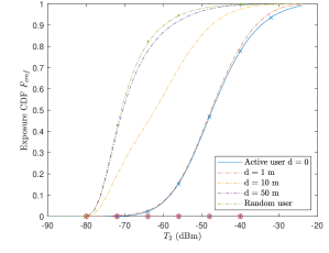
Figure 2: EMF exposure in a single-tier network with beamforming, active VS idle user at a distance $d$

IV-B Joint Metrics

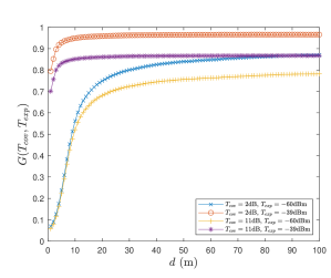
Figure 3: $\mathcal{J}^{SINR-IPD}(T_{c}^{UL},T_{exp};d)=\mathbb{P}\left[\text{SINR}(0)>T_{c}^{UL},\mathcal{P}(d)<T_{exp}\right]$

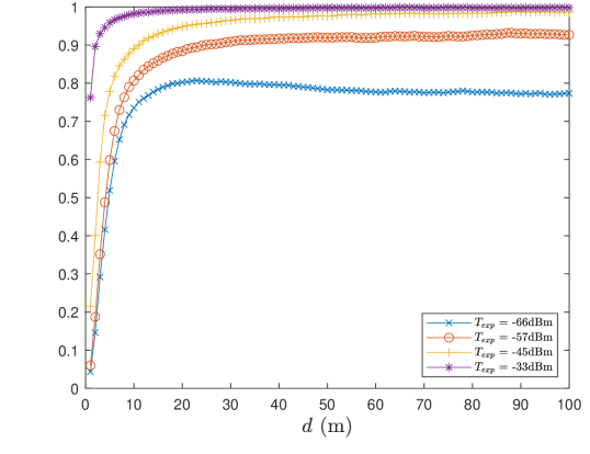
Figure 4: $\mathcal{J}^{SINR-IPD}(T_{exp}|T_{c}^{UL};d)=\mathbb{P}\left[\mathcal{P}(d)<T_{exp}|\text{SINR}(0)>\numprint[dB]{38}\right]$

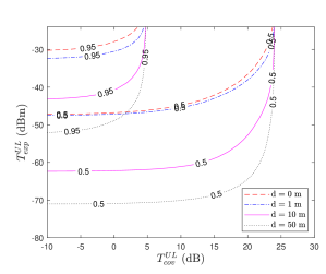
Figure 5: $\mathcal{J}^{SINR-IPD}(T_{c}^{UL},T_{exp};d)=\mathbb{P}\left[\text{SINR}(0)>T_{c}^{UL},\mathcal{P}(d)<T_{exp}\right]$

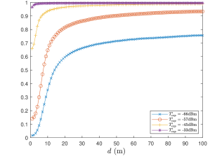
Figure 6: $\mathcal{J}^{SINR-IPD}(T^{\prime}_{exp}|T_{exp},T_{c};d)=\mathbb{P}\left[\mathcal{P}(d)<T^{\prime}_{exp}|\mathcal{P}(0)<\numprint[dBm]{-57},\text{SINR}(0)>\numprint[dB]{38}\right]$

V Conclusion

Appendix A Proof of the CF of the useful signal seen from the IU

If the angle $\delta_{0}$ is larger than 60^∘, the AU and the IU are not located in the same sector. The beam of the serving BS launched towards the AU has therefore no impact on the IU’s exposure. The CF of the useful signal from the point of view of the IU, conditioned on the distance location of the serving BS, should therefore consider these two cases in its definition:

$$\begin{split}\phi_{S}(q;d|X_{0})=\mathbb{E}_{|h|}\left[e^{jq\bar{P}_{r}(P_{0})G(\delta_{0})|h|^{2}}\mathds{1}\left[|\delta_{0}|\leq\pi/3\right]\right]\\ +\mathbb{E}_{|h|,\xi}\left[e^{jq\bar{P}_{r}(P_{0})G(\xi)|h|^{2}}\mathds{1}\left[|\delta_{0}|>\pi/3\right]\right].\end{split}$$ (27)

where $\mathds{1}[\cdot]$ is the indicator function. By applying the expectation operator $\mathbb{E}_{|h|}[\cdot]$ on the term for the case $\mathds{1}\left[|\delta_{0}|\leq\pi/3\right]$, we obtain

$$\mathbb{E}_{|h|}\left[e^{jq\bar{P}_{r}(P_{0})G(\delta_{0})|h|^{2}}\right]=\left(1-jq\bar{P}_{r}(P_{0})G(\delta_{0})/m\right)^{-m}.$$ (28)

For the term with the case $\mathds{1}\left[|\delta_{0}|>\pi/3\right]=1-\mathds{1}\left[|\delta_{0}|\leq\pi/3\right]$, let us develop the Talor series of the exponential function. Then, the infinite sum and the expectation operators can be swapped. Knowing that $\mathbb{E}_{|h|}\left[|h|^{2k}\right]=\frac{\Gamma(m+k)}{\Gamma(m)m^{k}}$, using the notation $z=jq\bar{P}_{r}(P_{0})$, we have

$$\begin{split}&\mathbb{E}_{|h|,\xi}\left[e^{zG(\xi)|h|^{2}}\right]=\mathbb{E}_{|h|,\xi}\left[\sum\limits_{k=0}^{\infty}\frac{\left(z\,G(\xi)|h|^{2}\right)^{k}}{k!}\right]\\ &=1+\sum\limits_{k=1}^{\infty}\frac{z^{k}}{k!}\mathbb{E}_{\xi}\left[G^{k}(\xi)\right]\frac{\Gamma(m+k)}{\Gamma(m)m^{k}}:=\eta_{S}(q|X_{0}).\end{split}$$ (29)

(16) is then obtained by inserting (28) and (29) in (27). Then $\eta_{S}(q|X_{0})$ can be developed separately for each gain function, using Proposition 1:

• (17) is obtained by inversely applying the definition of the binomial series.

• (19) is obtained by inversely applying the definition of the series expansion of the hypergeometric function ${}_{2}F_{1}(\cdot;\cdot;\cdot)$.

• The case of the Gaussian pattern is more complex. In that case, using (13), $\eta_{S}(q|X_{0})$ is given by

$$\begin{split}&\eta_{S}(q|X_{0})=\sum\limits_{k=0}^{\infty}\left(\frac{z\,g}{m}\right)^{k}\frac{\Gamma(m+k)}{\Gamma(m)k!}\\ &+\sum\limits_{k=1}^{\infty}\frac{3}{2}\frac{z^{k}}{k!}\frac{\Gamma(m+k)}{\Gamma(m)m^{k}}\sum\limits_{p=1}^{k}\!\binom{k}{p}(N-g)^{p}g^{k-p}\frac{\operatorname{erf}\left(\tfrac{\pi\sqrt{p\eta}}{3}\right)}{\sqrt{\pi p\eta}}\end{split}$$ (30)

The first term in (30) is solved by inversely applying the definition of the binomial series. The second term can be rewritten as

$$\begin{split}&\sum\limits_{p=1}^{\infty}\frac{3\operatorname{erf}\left(\tfrac{\pi\sqrt{p\eta}}{3}\right)}{2\sqrt{\pi p\eta}}(N-g)^{p}\sum\limits_{k=p}^{\infty}\!\frac{z^{k}}{k!}\frac{\Gamma(m+k)}{\Gamma(m)m^{k}}\binom{k}{p}g^{k-p}\\ &=\sum\limits_{p=1}^{\infty}\frac{3\operatorname{erf}\left(\tfrac{\pi\sqrt{p\eta}}{3}\right)}{2\sqrt{\pi p\eta}}(N-g)^{p}\frac{z^{p}}{p!}\frac{\Gamma(m+p)}{\Gamma(m)m^{p}}\left(1-\frac{z}{m}\right)^{-(m+p)}\end{split}$$ (31)

Replacing (31) in (30) gives (18) in Proposition 2.

Appendix B Proof of Proposition 3

The CF function of the interference of the active user at the origin is defined and commonly written as $\phi_{I}(q|r_{0})=\mathbb{E}_{I_{0}}\left[\exp(jq{I_{0}}(0))\right]$. Following from [20], and contrarily to the conventional procedure, the first step consists of taking first the expectation over the interferers’ locations, by means of the probability generating functional:

$$\begin{split}&\phi_{I}(q|R_{0})=\mathbb{E}_{I_{0}}\left[e^{jq{I_{0}}(0)}\right]\\ &\quad=\exp\left(-{\pi\lambda}\mathbb{E}_{\xi,|h|}\left[2\int_{R_{0}}^{\tau}\!\left(1-e^{jq{P}_{r}(r)}\right)r\,dr\right]\right)\\ &\quad=\exp\Bigg{(}-{\pi\lambda}\Bigg{(}\underbrace{\tau^{2}-R_{0}^{2}-\mathbb{E}_{\xi,|h|}\left[\int_{R_{0}}^{\tau}\!2e^{jq{P}_{r}(r)}r\,dr\right]}_{\eta_{I}(q|R_{0})}\Bigg{)}\Bigg{)}.\end{split}$$ (32)

By using the change of variable $t\to-jq{P}_{r}(r)$ and writing $\delta=2/\alpha$, the integral can be rewritten

$$\begin{split}&\int_{R_{0}}^{\tau}\!2e^{jq{P}_{r}(r)}r\,dr\\ &\quad=\delta\int_{-jq{P}_{r}(R_{0})}^{-jq{P}_{r}(\tau)}\!\left(jqP_{t}\kappa^{-1}G|h|^{2}\right)^{\delta}e^{-t}(-t)^{-1-\delta}\,dt\\ &\quad=\delta\left(-jqP_{t}\kappa^{-1}G|h|^{2}\right)^{\delta}\left[\Gamma(-\delta,-jqP_{r}(r)\right]_{r=R_{0}}^{r=\tau}.\end{split}$$ (33)

$\Gamma(a,z)$ is the upper incomplete Gamma function whose definition and expansion series are [49]

$$\Gamma(a,z)=\int_{z}^{\infty}{e^{-t}}{t^{a-1}}dt=\Gamma(a)-\sum\limits_{k=0}^{\infty}\frac{(-1)^{k}z^{a+k}}{k!(a+k)}.$$ (34)

Using this expansion series in (33) and inserting it in $\eta_{I}(q|R_{0})$ in (LABEL:eq:phiI0first) and letting $\Xi(r)=jq\bar{P}_{r}(r)$ gives

$$\eta_{I}(q|R_{0})=\left[r^{2}+\delta\left(\tau^{2}+z^{2}\right)\sum\limits_{k=0}^{\infty}\frac{\Xi^{k}(r)\mathbb{E}_{\xi,|h|}\!\left[G^{k}|h|^{2k}\right]}{k!(k-\delta)}\right]_{r=R_{0}}^{r=\tau}\!.$$

Extracting the terms $k=0$ and using $\mathbb{E}\left[|h|^{2k}\right]=\frac{\Gamma(m+k)}{\Gamma(m)m^{k}}$, gives after some simplifications

$$\eta_{I}(q|R_{0})=\delta\left[\left(r^{2}+z^{2}\right)\sum_{k=1}^{\infty}\frac{\mathbb{E}_{\xi}\!\left[G^{k}(\xi)\right]\Xi^{k}(r)}{k!(k-\delta)}\frac{\Gamma(m+k)}{\Gamma(m)m^{k}}\right]_{r=R_{0}}^{r=\tau}\!.$$ (35)

Similarly to what is done for $\eta_{S}(q|X_{0})$ in Appendix A, $\eta_{I}(q|R_{0})$ can be developed separately for each gain function, using Proposition 1. The expressions of $\eta_{I}(q|R_{0})$ for the flat-top and multi-cos patterns in Proposition 3 are obtained by using the series expansion of the generalized hypergeometric function ${}_{p}F_{q}(\cdot;\cdot)$. For case of the Gaussian pattern is again more complex. Using (13) and writing $\eta_{I}(q|r)$ such that $\eta_{I}(q|R_{0})=\left[\eta_{I}(q|r)]\right]_{r=R_{0}}^{r=\tau}$, we have

$$\begin{split}&\eta_{I}(q|r)=\delta\left(r^{2}+z^{2}\right)\sum\limits_{k=0}^{\infty}\left(\frac{\Xi(r)g}{m}\right)^{k}\!\frac{\Gamma(m+k)}{\Gamma(m)k!(k-\delta)}+r^{2}+z^{2}\\ &+\sum\limits_{k=1}^{\infty}\frac{3}{2}\frac{\Xi^{k}(r)\delta\left(r^{2}+z^{2}\right)\Gamma(m+k)}{\Gamma(m)m^{k}(k-\delta)k!}\sum\limits_{p=1}^{k}\!\binom{k}{p}(N-g)^{p}g^{k-p}\frac{\operatorname{erf}\left(\tfrac{\pi\sqrt{p\eta}}{3}\right)}{\sqrt{\pi p\eta}}\end{split}$$ (36)

The first term in (36) is solved by inversely applying the series expansion of ${}_{2}F_{1}(\cdot;\cdot;\cdot)$:

$$\sum\limits_{k=0}^{\infty}\left(\frac{\chi\,g}{m}\right)^{k}\frac{\Gamma(m+k)}{\Gamma(m)k!(k-\delta)}=-\frac{1}{\delta}{}_{2}F_{1}(-\delta,m;1-\delta;\frac{\chi g}{m}).$$

The term of the second line of (36) can be rewritten as

$$\begin{split}&\sum\limits_{p=1}^{\infty}\frac{3\operatorname{erf}\left(\tfrac{\pi\sqrt{p\eta}}{3}\right)}{2\sqrt{\pi p\eta}}(N-g)^{p}\sum\limits_{k=p}^{\infty}\!\frac{z^{k}}{k!}\frac{\Gamma(m+k)}{\Gamma(m)m^{k}(k-\delta)}\binom{k}{p}g^{k-p}\\ &=\sum\limits_{p=1}^{\infty}\frac{3\operatorname{erf}\left(\tfrac{\pi\sqrt{p\eta}}{3}\right)}{2\sqrt{\pi p\eta}}\left(\frac{N}{g}-1\right)^{p}\frac{\Gamma(p+m)}{\Gamma(m)p!}\\ &\qquad\times B\left(\frac{gz}{m};p-\delta,-p+1-m\right)\left(\frac{gz}{m}\right)^{\delta}\end{split}$$ (37)

where $B(\cdot;\cdot,\cdot)$ is the generalized beta function.

Appendix C Proof of Theorem 3

C-A General Form of the Metric

The fading coefficients affecting the links related to the two locations being independent, conditioned on the PP $\Psi$, the joint metric can be decomposed as

$$\mathcal{J}(T_{c},T_{e};d)=\mathbb{E}_{\Psi}\left[\mathbb{P}\left[\textrm{SINR}_{0}>T_{c}|\Psi\right]\,\mathbb{P}\left[\mathcal{P}^{IU}(d)<T_{e}|\Psi\right]\right].$$

The two factors in the above product can be developed using the Gil-Pelaez theorem. Using again the assumption of a CF of the interference identical for the AU and the IU, let $\phi_{\text{{SINR}}}(q,T_{c}|\Psi)=\phi_{S}(q;0|\Psi)\,\phi_{I}(-qT_{c}|\Psi)\,e^{-jqT_{c}\sigma^{2}}$ and $\phi_{E}^{IU}(q;d|\Psi)=\phi_{S}(q;d|\Psi)\,\phi_{I}(q|\Psi)\,e^{-jqT_{e}}$ be respectively the CFs of the signal and interference conditioned on $\Psi$. Using these notations, we get

$$\begin{split}\mathcal{J}(T_{c},T_{e};d)=\mathbb{E}_{\Psi}\left[\left(\frac{1}{2}+\int_{0}^{\infty}\textrm{Im}\!\left[\phi_{\text{{SINR}}}(q,T_{c}|\Psi)\right]\frac{1}{\pi q}dq\right)\right.\\ \left.\left(\frac{1}{2}-\int_{0}^{\infty}\textrm{Im}\!\left[\phi_{E}^{IU}(q^{\prime};d|\Psi)\,e^{-jq^{\prime}T_{e}}\right]\frac{1}{\pi q^{\prime}}dq\right)\right].\end{split}$$

By distributing the terms then the expectation operator, we get

$$\begin{split}\mathcal{J}(T_{c},T_{e};d)=-\frac{1}{4}+\frac{1}{2}\,\mathbb{E}_{\Psi}\Big{[}\underbrace{\frac{1}{2}+\int_{0}^{\infty}\textrm{Im}\!\left[\phi_{\text{{SINR}}}(q,T_{c}|\Psi)\right]\frac{1}{\pi q}\,dq}_{F_{cov}(T_{c}|\Psi)}\Big{]}\\ +\frac{1}{2}\,\mathbb{E}_{\Psi}\Big{[}\underbrace{\frac{1}{2}-\int_{0}^{\infty}\textrm{Im}\!\left[\phi_{E}^{IU}(q^{\prime};d|\Psi)\,e^{-jq^{\prime}T_{e}}\right]\frac{1}{\pi q^{\prime}}\,dq^{\prime}}_{F_{emf}^{IU}(T_{e};d|\Psi)}\Big{]}\\ -\frac{1}{\pi^{2}}\!\underbrace{\mathbb{E}_{\Psi}\Big{[}\int_{0}^{\infty}\!\textrm{Im}\!\left[\phi_{\text{{SINR}}}(q,T_{c}|\Psi)\right]\!\frac{dq}{q}\!\int_{0}^{\infty}\!\textrm{Im}\!\left[\phi_{E}^{IU}(q^{\prime};d|\Psi)\,e^{-jq^{\prime}T_{e}}\right]\!\frac{dq^{\prime}}{q^{\prime}}\Big{]}}_{\Upsilon(T_{c},T_{e};d)}.\end{split}$$

By applying the expectation operator, one has

$$\mathbb{E}_{\Psi}\left[F_{cov}(T_{c}|\Psi)\right]=F_{cov}(T_{c})$$

$$\mathbb{E}_{\Psi}\left[F_{emf}^{IU}(T_{e};d|\Psi)\right]=F_{emf}^{IU}(T_{e};d)$$

due to the motion-invariance of the H-PPP in $\mathbb{R}^{2}$, which gives the first line of Theorem 3.

C-B Decomposition of $\Upsilon(T_{c},T_{e};d)$

The expectation over $\Psi$ in the last expression of $\Upsilon(T_{c},T_{e};d)$ can be decomposed in the following manner:

$$\mathbb{E}_{\Psi}\left[\cdot\right]\to\mathbb{E}_{X_{0}}\left[\mathbb{E}_{\Psi\backslash\{X_{0}\}}\left[\cdot\right]\right]$$

where the coordinates of the serving BS $X_{0}$ are $(R_{0},\Theta_{0})$. Additionally, we write $\Psi^{*}=\Psi\backslash\{X_{0}\}$. Building up on these notations and using the PDF (1), we obtain

$$\Upsilon(T_{c},T_{e};d)=\frac{1}{2\pi}\int_{r_{e}}^{\tau}\int_{0}^{2\pi}\Upsilon(T_{c},T_{e};d|r_{0},\theta_{0})\,d\theta\,f_{R_{0}}(r_{0})\,dr_{0}.$$

where

$$\begin{split}&\Upsilon(T_{c},T_{e};d|R_{0},\Theta_{0})\\ &=\mathbb{E}_{\Psi^{*}}\Big{[}\int_{0}^{\infty}\textrm{Im}\Big{[}\phi_{I}(-qT_{c}|\Psi)\,\phi_{S}(q;0|\Psi)\,e^{-jqT_{c}\sigma^{2}}\Big{]}\frac{1}{q}dq\Big{.}\\ &\qquad\Big{.}\times\int_{0}^{\infty}\textrm{Im}\Big{[}\phi_{I}(q^{\prime}|\Psi)\,\phi_{S}(q^{\prime};d|\Psi)\,e^{-jq^{\prime}T_{e}}\Big{]}\frac{1}{q^{\prime}}dq^{\prime}\Big{]}\end{split}$$

Let $v_{1}\!=\!\phi_{S}(q;0|\Psi)\,e^{-jqT_{c}\sigma^{2}}$ and $v_{2}\!=\!\phi_{S}(q^{\prime};d|\Psi)\,e^{-jq^{\prime}T_{e}}$. By swapping the expectation and the integrals, following Fubini’s theorem, we obtain

$$\begin{split}&\Upsilon(T_{c},T_{e};d|R_{0},\Theta_{0})\\ &=\int_{0}^{\infty}\!\int_{0}^{\infty}\!\underbrace{\mathbb{E}_{\Psi^{*}}\!\left[\textrm{Im}\!\left[\phi_{I}(-qT_{c}|\Psi)v_{1}\right]\textrm{Im}\!\left[\phi_{I}(q^{\prime}|\Psi)v_{2}\right]\right]}_{\epsilon(q,q^{\prime};T_{c},T_{e},d|R_{0},\Theta_{0})}\!\frac{dq\,dq^{\prime}}{q\,q^{\prime}}.\end{split}$$ (38)

C-C Decomposition of $\epsilon(q,q^{\prime};T_{c},T_{e},d|r_{0},\theta_{0})$

Since $\phi_{S}$ does not depend on $\Psi^{*}$, by using $\textrm{Im}[x]=\frac{x-\bar{x}}{2}$ and $\text{Re}[x]=\frac{x+\bar{x}}{2}$, we obtain

$$\epsilon(q,q^{\prime};T_{c},T_{e},d|R_{0},\Theta_{0})\\ =\frac{1}{4}\,\mathbb{E}_{\Psi^{*}}\!\left[\left(\phi_{I}\left(-qT_{c}|\Psi\right)\,v_{1}-\bar{\phi_{I}}\left(-qT_{c}|\Psi\right)\,\bar{v_{1}}\right)\right.\\ \qquad\times\,\left.\left(\phi_{I}\left(q^{\prime}|\Psi\right)\,v_{2}-\bar{\phi_{I}}\left(q^{\prime}|\Psi\right)\,\bar{v_{2}}\right)\right]\\ =\frac{1}{4}\,\mathbb{E}_{\Psi^{*}}\!\left[\phi_{I}\left(-qT_{c}|\Psi\right)\,\phi_{I}\left(q^{\prime}|\Psi\right)\right]\,v_{1}\,v_{2}\\ -\frac{1}{4}\,\mathbb{E}_{\Psi^{*}}\!\left[\phi_{I}\left(-qT_{c}|\Psi\right)\,\bar{\phi_{I}}\left(q^{\prime}|\Psi\right)\right]\,v_{1}\,\bar{v_{2}}\\ -\frac{1}{4}\,\mathbb{E}_{\Psi^{*}}\!\left[\bar{\phi_{I}}\left(-qT_{c}|\Psi\right)\,\phi_{I}\left(q^{\prime}|\Psi\right)\right]\,\bar{v_{1}}\,v_{2}\\ +\frac{1}{4}\,\mathbb{E}_{\Psi^{*}}\!\left[\bar{\phi_{I}}\left(-qT_{c}|\Psi\right)\,\bar{\phi_{I}}\left(q^{\prime}|\Psi\right)\right]\,\bar{v_{1}}\,\bar{v_{2}}\\ =\frac{1}{2}\,\text{Re}\left[\gamma_{+}(q,q^{\prime}|r_{0})\,v_{1}\,v_{2}\right]-\frac{1}{2}\,\text{Re}\left[\gamma_{-}(q,q^{\prime}|r_{0})\,v_{1}\,\bar{v_{2}}\right]$$ (39)

where we define

$$\gamma_{+}(q,q^{\prime}|r_{0})=\mathbb{E}_{\Psi^{*}}\!\left[\phi_{I}\left(q|\Psi\right)\,\phi_{I}\left(q^{\prime}|\Psi\right)\right]$$ (40)

and

$$\gamma_{-}(q,q^{\prime}|r_{0})=\mathbb{E}_{\Psi^{*}}\!\left[\phi_{I}\left(q|\Psi\right)\,\bar{\phi_{I}}\left(q^{\prime}|\Psi\right)\right].$$ (41)

C-D Decomposition of $\gamma_{+}$ and $\gamma_{-}$

The methodology employed to calculate the expressions of $\gamma_{+}$ and $\gamma_{-}$ aligns with the approach detailed in Appendix C of [47] for the identical network pertaining to a PU. The only modification required lies in adjusting the lower bound of the integral in equation (30), substituting $r_{0}$ for $r_{e}$.

References

- [1] M. Rumney, “5G Safety : A scientific response to an increasingly polarized debate,” COST Action CA15104: Fourth and Final Scientific Annual Report (TD(19)11003), 2019.
- [2] ICNIRP, “ICNIRP Guidelines for Limiting Exposure to Electromagnetic Fields ( to ),” Health Physics, vol. 118, pp. 483–524, 2020.
- [3] ANFR, “Evaluation de l’exposition du public aux ondes électromagnétiques 5G Volet 1 : présentation générale de la 5G,” pp. 1–17, 2019.
- [4] E. C. Strinati et al., “Wireless environment as a service enabled by reconfigurable intelligent surfaces: The rise-6g perspective,” in 2021 Joint European Conference on Networks and Communications & 6G Summit (EuCNC/6G Summit), 2021, pp. 562–567.
- [5] S. Aerts, L. Verloock, M. Van den Bossche, and J. Wout, “In-situ metingen van radiofrequente elektromagnetische velden in de nabijheid van een 5G NR-basisstation,” IMEC - WAVES - Ghent University, Tech. Rep., March 2020.
- [6] G. Vermeeren et al., “Low EMF exposure future networks D2. 8 global wireless exposure metric definition,” LEXNET Consortium, Tech. Rep., 2015.
- [7] S. Aerts, L. Verloock, M. Van Den Bossche, D. Colombi, L. Martens, C. Törnevik, and W. Joseph, “In-situ Measurement Methodology for the Assessment of 5G NR Massive MIMO Base Station Exposure at Sub-6 GHz Frequencies,” IEEE Access, vol. 7, pp. 184 658–184 667, 2019.
- [8] “Study of the contribution of 5G to the general public exposure to electromagnetic waves,” Agence Nationale des Fréquences, Tech. Rep., 2021.
- [9] L. Chiaraviglio, S. Rossetti, S. Saida, S. Bartoletti, and N. Blefari-Melazzi, ““Pencil Beamforming Increases Human Exposure to ElectroMagnetic Fields”: True or False?” IEEE Access, vol. 9, pp. 25 158–25 171, 2021.
- [10] M. S. Elbasheir, R. A. Saeed, A. A. Z. Ibrahim, S. Edam, F. Hashim, and S. M. E. Fadul, “A Review of EMF Radiation for 5G Mobile Communication Systems,” in 2021 IEEE Asia-Pacific Conference on Applied Electromagnetics (APACE), 2021, pp. 1–6.
- [11] I. Patsouras et al., “Beyond 5G/6G EMF Considerations,” Jul. 2023. [Online]. Available: https://doi.org/10.5281/zenodo.8099834
- [12] H. B. A. Sidi and Z. Altman, “Small Cells’ Deployment Strategy and Self-Optimization for EMF Exposure Reduction in HetNets,” IEEE Transactions on Vehicular Technology, vol. 65, no. 9, pp. 7184–7194, 2015.
- [13] A. T. Ajibare, D. Ramotsoela, L. A. Akinyemi, and S. O. Oladejo, “RF EMF Radiation Exposure Assessment of 5G Networks: Analysis, Computation and Mitigation Methods,” in 2021 IEEE AFRICON, 2021, pp. 1–6.
- [14] E. C. Strinati et al., “Reconfigurable, Intelligent, and Sustainable Wireless Environments for 6G Smart Connectivity,” IEEE Communications Magazine, vol. 59, no. 10, pp. 99–105, 2021.
- [15] D.-T. Phan-Huy, Y. Bénédic, S. H. Gonzalez, and P. Ratajczak, “Creating and Operating Areas With Reduced Electromagnetic Field Exposure Thanks to Reconfigurable Intelligent Surfaces,” in 2022 IEEE 23rd International Workshop on Signal Processing Advances in Wireless Communication (SPAWC), 2022, pp. 1–5.
- [16] H. Ibraiwish, A. Elzanaty, Y. H. Al-Badarneh, and M.-S. Alouini, “EMF-Aware Cellular Networks in RIS-Assisted Environments,” IEEE Communications Letters, vol. 26, no. 1, pp. 123–127, 2022.
- [17] F. Baccelli, M. Klein, M. Lebourges, and S. A. Zuyev, “Stochastic geometry and architecture of communication networks,” Telecommunication Systems, vol. 7, pp. 209–227, 1997.
- [18] C.-H. Lee, C.-Y. Shih, and Y.-S. Chen, “Stochastic Geometry Based Models for Modeling Cellular Networks in Urban Areas,” Wirel. Netw., vol. 19, no. 6, p. 1063–1072, aug 2013.
- [19] D. Maamari, N. Devroye, and D. Tuninetti, “Coverage in mmWave Cellular Networks With Base Station Co-Operation,” IEEE Transactions on Wireless Communications, vol. 15, no. 4, pp. 2981–2994, 2016.
- [20] X. Yu, J. Zhang, M. Haenggi, and K. B. Letaief, “Coverage Analysis for Millimeter Wave Networks: The Impact of Directional Antenna Arrays,” IEEE Journal on Selected Areas in Communications, vol. 35, no. 7, pp. 1498–1512, 2017.
- [21] M. Di Renzo, “Stochastic Geometry Modeling and Analysis of Multi-Tier Millimeter Wave Cellular Networks,” IEEE Transactions on Wireless Communications, vol. 14, no. 9, pp. 5038–5057, 2015.
- [22] S. S. Kalamkar, F. Baccelli, F. M. Abinader, A. S. M. Fani, and L. G. U. Garcia, “Beam Management in 5G: A Stochastic Geometry Analysis,” IEEE Transactions on Wireless Communications, vol. 21, no. 4, pp. 2275–2290, 2022.
- [23] Y. Chen, Q. Zhu, C. Guo, and C. Feng, “On the Performance of Downlink Non-Orthogonal Multiple Access Wireless Networks With Directional Beamforming and Limit of the User Number,” IEEE Transactions on Vehicular Technology, vol. 70, no. 7, pp. 6696–6712, 2021.
- [24] L. Yang, F.-C. Zheng, and S. Jin, “SINR Meta Distribution for mmWave Heterogeneous Networks Under Varying Queue Status: A Spatio-Temporal Analysis,” IEEE Transactions on Vehicular Technology, vol. 71, no. 12, pp. 13 281–13 298, 2022.
- [25] R. Kovalchukov, D. Moltchanov, A. Samuylov, A. Ometov, S. Andreev, Y. Koucheryavy, and K. Samouylov, “Evaluating SIR in 3D Millimeter-Wave Deployments: Direct Modeling and Feasible Approximations,” IEEE Transactions on Wireless Communications, vol. 18, no. 2, pp. 879–896, 2019.
- [26] Y. Wu, J. Kokkoniemi, C. Han, and M. Juntti, “Interference and Coverage Analysis for Terahertz Networks With Indoor Blockage Effects and Line-of-Sight Access Point Association,” IEEE Transactions on Wireless Communications, vol. 20, no. 3, pp. 1472–1486, 2021.
- [27] N. A. Muhammad, N. Seman, and N. I. A. Apandi, “Effect of Directional Antenna Arrays on Millimeter Wave Cellular Networks,” in 2022 International Symposium on Antennas and Propagation (ISAP), 2022, pp. 205–206.
- [28] Y. Nabil, H. ElSawy, S. Al–Dharrab, H. Attia, and H. Mostafa, “A Stochastic Geometry Analysis for Joint Radar Communication System in Millimeter-wave Band,” in ICC 2023 - IEEE International Conference on Communications, 2023, pp. 5849–5854.
- [29] A. Thornburg and R. W. Heath, “Ergodic capacity in mmWave ad hoc network with imperfect beam alignment,” in MILCOM 2015 - 2015 IEEE Military Communications Conference, 2015, pp. 1479–1484.
- [30] M. Rebato, J. Park, P. Popovski, E. De Carvalho, and M. Zorzi, “Stochastic Geometric Coverage Analysis in mmWave Cellular Networks With Realistic Channel and Antenna Radiation Models,” IEEE Transactions on Communications, vol. 67, no. 5, pp. 3736–3752, 2019.
- [31] R. Aghazadeh Ayoubi and U. Spagnolini, “Performance of Dense Wireless Networks in 5G and beyond Using Stochastic Geometry,” Mathematics, vol. 10, no. 7, 2022. [Online]. Available: https://www.mdpi.com/2227-7390/10/7/1156
- [32] T. A. Khan, A. Alkhateeb, and R. W. Heath, “Millimeter wave energy harvesting,” IEEE Transactions on Wireless Communications, vol. 15, no. 9, pp. 6048–6062, 2016.
- [33] J. Guo, X. Zhou, and S. Durrani, “Wireless power transfer via mmwave power beacons with directional beamforming,” IEEE Wireless Communications Letters, vol. 8, no. 1, pp. 17–20, 2019.
- [34] N. Deng and M. Haenggi, “Energy Correlation Coefficient in Wirelessly Powered Networks with Energy Beamforming,” in ICC 2021 - IEEE International Conference on Communications, 2021, pp. 1–6.
- [35] M. Di Renzo and W. Lu, “System-Level Analysis and Optimization of Cellular Networks With Simultaneous Wireless Information and Power Transfer: Stochastic Geometry Modeling,” IEEE Transactions on Vehicular Technology, vol. 66, no. 3, pp. 2251–2275, 2017.
- [36] T. Tu Lam, M. Di Renzo, and J. P. Coon, “System-Level Analysis of SWIPT MIMO Cellular Networks,” IEEE Communications Letters, vol. 20, no. 10, pp. 2011–2014, 2016.
- [37] M. Wang, C. Zhang, X. Chen, and S. Tang, “Performance Analysis of Millimeter Wave Wireless Power Transfer With Imperfect Beam Alignment,” IEEE Transactions on Vehicular Technology, vol. 70, no. 3, pp. 2605–2618, 2021.
- [38] M. Al Hajj, S. Wang, L. Thanh Tu, S. Azzi, and J. Wiart, “A Statistical Estimation of 5G Massive MIMO Networks’ Exposure Using Stochastic Geometry in mmWave Bands,” Applied Sciences, vol. 10, no. 23, 2020.
- [39] Q. Gontier, L. Petrillo, F. Rottenberg, F. Horlin, J. Wiart, C. Oestges, and P. De Doncker, “A Stochastic Geometry Approach to EMF Exposure Modeling,” IEEE Access, vol. 9, pp. 91 777–91 787, 2021.
- [40] M. A. Hajj, S. Wang, and J. Wiart, “Characterization of EMF Exposure in Massive MIMO Antenna Networks with Max-Min Fairness Power Control,” in 2022 16th European Conference on Antennas and Propagation (EuCAP), 2022, pp. 1–5.
- [41] N. A. Muhammad, N. Seman, N. I. A. Apandi, C. T. Han, Y. Li, and O. Elijah, “Stochastic Geometry Analysis of Electromagnetic Field Exposure in Coexisting Sub-6 GHz and Millimeter Wave Networks,” IEEE Access, vol. 9, pp. 112 780–112 791, 2021.
- [42] Q. Gontier, C. Wiame, S. Wang, M. Di Renzo, J. Wiart, F. Horlin, C. Tsigros, C. Oestges, and P. De Doncker, “Joint Metrics for EMF Exposure and Coverage in Real-World Homogeneous and Inhomogeneous Cellular Networks,” 2023. [Online]. Available: https://arxiv.org/abs/2302.03559
- [43] C. Wiame, S. Demey, L. Vandendorpe, P. De Doncker, and C. Oestges, “Joint Data Rate and EMF Exposure Analysis in Manhattan Environments: Stochastic Geometry and Ray Tracing Approaches,” IEEE Transactions on Vehicular Technology, vol. 73, no. 1, pp. 894–908, 2024.
- [44] C. Wiame, C. Oestges, and L. Vandendorpe, “Joint data rate and EMF exposure analysis in user-centric cell-free massive MIMO networks,” 2023, submitted. [Online]. Available: https://arxiv.org/abs/2301.11127
- [45] Q. Gontier, C. Wiame, J. Wiart, F. Horlin, C. Tsigros, C. Oestges, and P. D. Doncker, “On the uplink and downlink emf exposure and coverage in dense cellular networks: A stochastic geometry approach,” 2023.
- [46] L. Chen, A. Elzanaty, M. A. Kishk, L. Chiaraviglio, and M.-S. Alouini, “Joint Uplink and Downlink EMF Exposure: Performance Analysis and Design Insights,” IEEE Transactions on Wireless Communications, 2023.
- [47] Q. Gontier, C. Wiame, F. Horlin, C. Tsigros, C. Oestges, and P. De Doncker, “Meta Distribution of Passive Electromagnetic Field Exposure in Cellular Networks,” 2024, unpublished. [Online]. Available: https://arxiv.org/abs/2302.03559
- [48] J. Gil-Pelaez, “Note on the inversion theorem,” Biometrika, vol. 38, no. 3-4, pp. 481–482, 12 1951.
- [49] I. Gradshteyn and I. Ryzhik, “Use of the Tables,” in Table of Integrals, Series, and Products (Eighth Edition), D. Zwillinger, V. Moll, I. Gradshteyn, and I. Ryzhik, Eds. Boston: Academic Press, 2014, pp. xxix–xxxvi.