Gradient-Congruity Guided Federated Sparse Training

Abstract

Edge computing allows artificial intelligence and machine learning models to be deployed on edge devices, where they can learn from local data and collaborate to form a global model. Federated learning (FL) is a distributed machine learning technique that facilitates this process while preserving data privacy. However, FL also faces challenges such as high computational and communication costs regarding resource-constrained devices, and poor generalization performance due to the heterogeneity of data across edge clients and the presence of out-of-distribution data. In this paper, we propose the Gradient-Congruity Guided Federated Sparse Training (FedSGC), a novel method that integrates dynamic sparse training and gradient congruity inspection into federated learning framework to address these issues. Our method leverages the idea that the neurons, in which the associated gradients with conflicting directions with respect to the global model contain irrelevant or less generalized information for other clients, and could be pruned during the sparse training process. Conversely, the neurons where the associated gradients with consistent directions could be grown in a higher priority. In this way, FedSGC can greatly reduce the local computation and communication overheads while, at the same time, enhancing the generalization abilities of FL. We evaluate our method on challenging non-i.i.d settings and show that it achieves competitive accuracy with state-of-the-art FL methods across various scenarios while minimizing computation and communication costs.

1 Introduction

Machine learning has seen significant success in various fields, but traditional centralized training methods pose challenges due to the need for large data sets, high costs, and potential privacy risks. Federated Learning (FL) Yang et al. (2019); McMahan et al. (2017) addresses these issues by allowing multiple parties to collaboratively learn a model without sharing private data. In an FL system, each party trains a local model on their own data, and the weights or gradients are sent to a central server for aggregation. The server updates the global model and sends it back for further training.

FL is ideal for edge computing applications involving distributed devices with limited resources. However, training Deep Neural Networks (DNNs) on these devices presents challenges related to resource efficiency and data heterogeneity. Edge devices may have limited resources for local training and communication with the central server, and they may exhibit heterogeneous data distributions, affecting the generalization performance of FL.

Model compression techniques have been proposed to address resource efficiency, involving the transmission of a compressed parameter/gradient vector between clients and servers Wu et al. (2022); Chen et al. (2021). However, this only reduces communication workload and does not create a smaller, more efficient model. The lottery ticket hypothesis Frankle et al. (2020) suggests that dense neural networks contain sparse subnetworks that can achieve the same accuracy as the original model when trained alone. Some researchers aim to extract a lightweight model from the original model for more efficient client-side training Mugunthan et al. (2022); Li et al. (2021a); Tamirisa et al. (2023), but these methods may impose significant computation and communication overheads and neglect the large data heterogeneity across edge clients.

Regarding the issue of data heterogeneity issue in federated learning, many algorithmic solutions have been proposed in the literature (e.g., Acar et al. (2021); Karimireddy et al. (2020); Li et al. (2021b); Dai et al. (2023)). These strategies add proximal terms to the objective function to regularize local updates with respect to the global model. However, these methods limit local convergence potential and the amount of novel information per communication round, and may not consistently improve performance across different non-IID settings. Some alternative approaches propose personalized federated learning, which trains individual client models, or shares a small subset of an auxiliary dataset with clients to construct a more balanced IID data distribution. However, these methods often overlook client resource constraints and may even incur significant client compute and/or memory overheads.

In this paper, we propose to jointly address the aforementioned limitations with a novel federated learning (FL) framework called Federated Sparse Gradient Congruity (FedSGC). FedSGC integrates dynamic sparse training and gradient congruity inspection Yu et al. (2020); Mansilla et al. (2021); Tian et al. (2023) (i.e., to inspect whether gradient conflicts exist across different data sources) to enable efficient on-device computation and in-network communication for edge devices in federated learning. To be more specific, we propose a novel prune-and-grow mechanism by examining the gradients across different clients, where client’s local training gradients with conflicting directions with respect to the global model contain irrelevant or less generalized information for other clients and could be pruned during the sparse training process, and conversely, gradients with consistent directions with the global model’s learning direction could be kept by assigning a higher priority for regrowth of the pruned neurons, thereby fostering the learning of invariant knowledge.

2 Related Work

Federated Learning. Federated learning algorithms aim to obtain a global model that minimizes the training loss across all clients. Each client $j$ has a small set of local data $D_{j}$ for local training, but to preserve user privacy, clients do not share their local data, where the process can be formulated as $\min_{w}f(w)=\sum_{k=1}^{K}p_{k}F_{k}(w)$, where $F_{k}(w)$ denotes the objective of the deep learning model on the $k$-th client, $K$ is the set of clients, $p_{k}>0$, and $\sum_{k}p_{k}=1$. In practice, one can set $p_{k}=n_{k}/n$, where $n_{k}$ and $n$ denote the number of data points in the $k$-th client and the total number of data points, respectively. It is worth noting that federated learning is different from the traditional distributed learning scenario where data partitions are assumed to be i.i.d., meaning that they are generated from the same memoryless stochastic process. However, this assumption does not hold in federated learning. Instead, data can often be heterogeneous among clients.

In the FedAvg McMahan et al. (2017) family of algorithms, training proceeds in communication rounds. At the beginning of each round $r$, the server selects a subset of clients $C^{r}$, $C^{r}\subseteq K$, and sends the current server model parameters $\theta^{i}$ to the clients. Each client $c\in C^{r}$ performs $E$ epochs of training using the received model parameters on its local data to produce updated parameters $\theta^{r}_{c}$, which are then uploaded to the server. The server then updates the global model with a weighted average of the sampled clients’ parameters to produce $\theta^{r+1}$ for the next round.

Sparse Training. Sparse training performs training and pruning simultaneously by adding a sparsity regularization term to the loss function, producing structured sparsity. Sparse training with dynamic sparsity, also known as Dynamic Sparse Training (DST), is a recent research direction that aims at accelerating the training of neural networks without sacrificing performance. A neural network is initialized with a random sparse topology from scratch. The sparse topology (connectivity) and the weights are jointly optimized during training. During training, the sparse topology is changed periodically through a prune-and-grow cycle, where a fraction of the parameters are pruned, and the same portion is regrown among different neurons. An update schedule determines the frequency of topology updates. Many DST works have been proposed, focusing on improving the performance of sparse training for supervised image classification tasks by introducing different criteria for neuron growth Mostafa & Wang (2019); Evci et al. (2020). DST has demonstrated its success in many fields, such as continual learning Sokar et al. (2021a), feature selection Atashgahi et al. (2022), ensembling Liu et al. (2021), adversarial training Özdenizci & Legenstein (2021), and deep reinforcement learning Sokar et al. (2021b). FedDST Bibikar et al. (2022), which is closely related to our research, is based on the foundation of RigL Evci et al. (2020), thereby facilitating computational and communicational efficiency in FL environments. By adopting the gradient magnitude, which was utilized in the original RigL work for directing the pruning and growth process, with mask votes and a sparse weighted average mechanism, it can stabilize learning updates, thereby enhancing the robustness and effectiveness of the global model. However, it does not specifically address the issue of data heterogeneity and exhibits limitations in handling severe data heterogeneity.

3 Methodology

We adopt a federated learning setting based on the common FedAvg-like formulation $\min_{w}f(w)$. Instead of sending the full dense parameters $\theta^{r}_{j}$ to the central server at each round $r$, each client $j$ only uploads the sparse parameters along with a bit mask $(\theta^{r}_{j},m^{r}_{j})$. The bit mask has the same shape as the parameter to indicate whether the parameter at the corresponding index is zero or not.

The central server aggregates the parameters and masks from all clients to produce the global parameters and direction mask $(\theta^{r+1},d^{r+1})$ for the next round, along with the parameter mask $m^{r+1}$. These are then passed to the selected clients for the next round. The selected clients use the received parameters and direction mask to perform local sparse training. Following Evci et al. (2020), each client maintains a target overall sparsity $S=\frac{\sum_{l}s^{l}W^{l}}{W},S\in[0,1),$ where $l$ denotes the $l^{th}$ layer of the network and $W^{l}$ is the number of parameters in that layer. Each layer may have a different layer sparsity $s^{l}$, which is defined as the ratio of zero parameters to the total number of parameters in that layer, $s^{l}\in[0,1)$. We adopt Erdös-Rényi Kernel as the layer sparsity distribution ($s^{l}$) across the network, which is a modified version of Erdös-Rényi formulation Mocanu et al. (2018), to generally allocate higher sparsities to the layers with more parameters while allocating lower sparsities to the smaller ones.

3.1 The Prune-and-Grow Mechanism for Sparsity Training

The dynamic sparse training consists of two phases: learning and re-adjusting. In the learning phase, each client updates the masked parameters using its local training data through standard backpropagation. Parameters with zero mask values remain unchanged and do not join the training. In the re-adjusting stage, each selected client will periodically re-adjust/update its parameter mask to enable dynamic sparsity. The re-adjusting stage is triggered by the global server: starting from the initial training round, for every $\Delta R$ rounds till $R_{end}$, the global server requests for mask re-adjustment. Each client records its cumulative training epochs since the start of the first round and re-adjusts its mask every $\Delta T$ epochs until it reaches $T^{end}_{c}$ i.e. the total expected training epochs of the client $c$. The re-adjusting process has two steps: pruning and growing. In the pruning step, for each layer, given the target layer sparsity $s^{l}$, each client $c$ prunes its layer parameters to a slightly higher sparsity $\overline{s}^{l}_{c}=s^{l}+\sigma_{i}(1-s^{l}_{c})$, where $\sigma_{c}$ is a factor that controls the level of over-pruning, i.e., $k=\overline{s}^{l}_{c}N^{l}$ parameters will be pruned (mask set to 0) in total. Inspired by Evci et al. (2020), we also set $\sigma_{c}$ to be a periodic variable along the federated learning process in our work as $\sigma_{c}=\frac{\alpha}{2}(1+cos(\frac{t^{c}\pi}{T_{c}^{end}})),\quad\sigma_{c}\in[0,\alpha],$ where $\alpha$ is a hyper-parameter and $t_{c}$ is the current cumulative training epochs of client $c$. This means that each client prunes more parameters at the beginning than in the middle. In the growing step, we need to grow some neurons back (corresponding mask values set from 0 to 1) to achieve the target sparsity level. That means for each layer, we need to grow $\hat{k}$ parameters, where $\hat{k}=(\hat{s}^{l}-s^{l})*N^{j}$. We will discuss how we select which neurons to grow in the next section. Through the prune-and-grow cycle, the mask space for sparsity neural network training adaptively changes over time.

3.2 Gradient guided Pruning and Growing

Our main contribution is to propose a novel criterion for pruning and growing neurons in sparse neural networks. Unlike previous methods (e.g., Atashgahi et al. (2022)) that grow connections randomly without considering the issue of data heterogeneity, we design our criterion specifically for federated learning settings, where we leverage a global pseudo-gradientYao et al. (2019) direction map to optimize the network topology. The global direction map indicates the direction of the change in the global parameters after each round of aggregation, i.e. $d^{r+1}=sign(\theta^{r+1}-\theta^{r})$. We illustrate the training process of our approach in Algorithm 1 in the appendix.

Prune criterion. On the client-$c$ side, we select the parameters that have local pseudo-gradient of opposite sign from the global direction and then sort them by their weight absolute value in ascending order. We first prune the first $\lambda k$ of them. i.e.

$$K_{guided}=ArgTopK(-|\theta^{l}_{[i|d^{r}=-sign({\Delta_{c}^{r}})]}|,\lambda k),$$ (1)

where we follow Evci et al. (2020) to treat the layer parameter as a one-dimensional vector, $i$ is the neuron/parameter index in the vector, and the function $ArgTopK$ returns the indices of the top-k elements in the vector. $\Delta_{c}^{r}=\theta^{r,t}_{c}-\theta^{r,0}_{c}$ denotes the local pseudo-gradient of client $c$ at the current iteration step $t$ of round $r$, $\lambda$ is a hyper-parameter that controls the proportion of pruning guided by the gradient congruity. The motivation here is that the neurons where the associated global and local gradients are incongruous (i.e., the sign of global and local gradients are different) are less likely to be generalized across heterogeneous data Mansilla et al. (2021). For the remaining neurons (i.e., neurons not in $K_{guided}$) to be pruned, we use the magnitude of the parameters only, i.e.,

$$K_{mag}=ArgTopK(-|\theta^{l}_{[i\notin K_{guided}]}|,(1-\lambda)k).$$ (2)

By pruning in this order, we prioritize pruning those with opposite directions while generally pruning by weight magnitude. Finally, we pruned parameters with indices in $K_{guided}\cup K_{mag}$.

Grow criterion. Similar to the pruning stage, we also adopt a prioritized approach to growing neurons. Initially, we grow the neurons that have the largest magnitude of loss gradient, and at the same time, have the same learning direction sign as the global direction, i.e.,

$$\hat{K}_{guided}=ArgTopK(|{\nabla}^{l}_{[i|d^{r}=sign({\Delta_{c}^{r,t}})]}|,\lambda\hat{k}),$$ (3)

where we grow the neurons that the associated direction of global and local gradient are congruent (i.e., $i|d^{r}=sign({\Delta_{c}^{r}})$, where $\Delta_{c}^{r}=\theta^{r,t}_{c}-\theta^{r,0}_{c}$ is the pseudo gradient of client $c$ at current iteration $t$ of round $r$, $i$ is the neuron index). Such neurons are safer to be grown as we expect them to be better generalized across clients with heterogeneous data Mansilla et al. (2021). For the remaining neurons (i.e., neurons not in $K_{guided}$) to be grown, we use the loss gradient magnitude given as

$$\hat{K}_{mag}=ArgTopK(|{\nabla}^{l}_{[i\notin\hat{K}_{guided}]}|,(1-\lambda)\hat{k}).$$ (4)

Finally, in the growing step, we grow neurons with indices in $\hat{K}_{guided}\cup\hat{K}_{mag}$.

3.3 Global Aggregation

When the central server receives the sparse parameters and masks from the clients, we perform a sparse weighted average to aggregate them as follows:

$$\theta^{r+\frac{1}{2}}=\frac{\sum_{c\in C^{r}}n_{c}\theta^{r}_{c}m^{r}_{c}+n_{rest}\theta^{r}m^{r}}{\sum_{c\in C^{r}}n_{c}m^{r}_{c}+n_{rest}m^{r}}, n_{rest}=n-\sum_{c\in C^{r}}n_{c},$$ (5)

$$\theta^{r+1}=prune\big{(}ArgTopK(-|\theta^{r+\frac{1}{2}}|,\tilde{k})\big{)},$$

Different from FedDST, in the central aggregation phase, we still consider the parameters and masks that are held by those clients who do not participate, as we find that updating the global model only by partially selected clients’ learning results may lead to unstable performance of the global model.

In this process, neurons that are zero-masked by all clients get pruned globally. In most cases, the global model sparsity after aggregation may be lower than the target sparsity $S$ since we use OR logic to aggregate the client masks. In such case, we prune some additional neurons with the smallest absolute value of the aggregated weights, i.e. $ArgTopK_{i}(-|\theta^{r+\frac{1}{2}}|,\tilde{k})$, where $\tilde{k}$ is the number of neurons to be pruned. This again helps us achieve the target sparsity $S$ and obtain the final global parameters $\theta^{r+1}$.

4 Experiments

In this section, we evaluate our proposed FedSGC on two benchmark datasets: MNIST , CIFAR-10. Our evaluation primarily focuses on comparing FedSGC with two SoTA FL methods that utilize pruning techniques: FedDST Bibikar et al. (2022) and PruneFL Jiang et al. (2022). We also adapt GraSP Wang et al. (2020) into FL setting as another baseline. We skip LotteryFL Li et al. (2020) as it is designed for Personalized FL setting. We assess the performance of these methods while considering communication costs. To reflect a challenging data heterogeneity environment, we create a highly non-IID data distribution among clients, following the same non-iid partition strategy as in FedAvg, where most client only has data from two classes. We also adopt the Dirichlet distribution with parameter $\beta$ to distribute the CIFAR-10 to simulate more relaxing but realistic heterogeneity.

4.1 Results on MNIST

Implementation. We select 100 clients from the MNIST dataset and randomly choose 10 clients to participate in each round of federated training. All methods are training for 400 federated rounds, 5 local epochs each round. We first sort the MNIST samples by label and split them into 200 shards of size 300. Each client is assigned two shards, resulting in pathological non-IID MNIST dataset partitions, where most clients only have data from two classes. resulting in a pathological non-IID partition where most clients only have data from two classes. For the federated training settings, we adopt the same CNN architecture and local training algorithm as in FedDST. The CNN consists of two 5x5 convolution layers (the first with 10 channels, the second with 20), a fully connected layer with 50 units and ReLU activation, and a final softmax output layer. The local training is performed via vanilla SGD with a learning rate of $lr=0.001$ and batch size of 50.

MNIST	Best accuracy encountered at
	cumulative upload capacity [MiB]
Method	100	200	400	800
FedAvg	21.3	45.2	73.4	81.3
FedProx	23.5	58.3	74.3	82.0
PruneFL	18.1	40.2	60.7	75.3
GraSP	20.2	42.4	66.1	70.3
FedDST	22.4	55.4	75.1	79.9
FedDSTμ=1.0	17.3	43.7	71.1	78.1
FedSGC	19.2	59.7	77.7	84.4
FedSGCμ=1.0	19.6	46.9	74.4	83.3

Table 1: On pathological non-iid MNIST. We fix $S=0.8,\alpha=0.5,\Delta R=20,\Delta T=20,\lambda=0.01$

CIFAR10	Best accuracy encountered at
	cumulative upload capacity [MiB]
Method	50	100	200	400
FedAvg	18.3	22.5	31.7	35.2
FedProx	14.9	22.3	24.0	34.3
PruneFL	19.3	21.3	30.9	36.0
GraSP	21.3	24.3	30.5	34.9
FedDST	28.5	36.2	38.6	40.1
FedDSTμ=0.1	30.5	35.2	37.2	41.2
FedSGC	33.3	36.6	41.1	44.6
FedSGCμ=0.1	32.3	36.0	40.2	43.5

Table 2: On pathological non-iid CIFAR-10. We fix $S=0.8,\alpha=0.01,\Delta R=20,\Delta T=10,\lambda=0.01$

Figure 1: Results on pathological non-iid MNIST dataset.

Figure 2: Results on pathological non-iid MNIST dataset of different sparsity.

Result analysis. We compared the accuracy of each method on challenging pathological partitions with a fixed upload bandwidth. The results are shown in Table 2 and Figure 2. PruneFL and GraSP were excluded due to their high bandwidth consumption. Our FedSGC outperformed other methods in accuracy and convergence speed, despite not excelling at the initial stage, likely due to the model’s random initialization. FedSGC quickly reached over 80% accuracy and achieved the highest accuracy within a cumulative upload bandwidth of around 840MiB. It also proved compatible with other FL regularization terms like FedProx, achieving better results than other baselines.

Comparison at different Sparsity Levels. We tested FedSGC’s robustness and efficacy at sparsity levels 0.6, 0.7 and 0.8, maintaining other parameters and settings. Figure 1 displays the results, showing FedSGC consistently outperforming FedDST across sparsity levels, yielding superior performance under identical upload capacity. FedSGC exhibits optimal performance at higher sparsity levels, suggesting the importance of effective neuron pruning and growth, to which gradient congruity-guided FedSGC significantly contributes.

4.2 Results on CIFAR10

Implementation. We use the same data partition setttings as for MNIST. We follow FedAvg to use the network architecture from the TensorFlow official tutorial google (1999) , which is a CNN with three 5x5 convolution layers (the first with 32 channels, the second and third with 64), a fully connected layer with 1024 units and ReLU activation, and a final softmax output layer. The local training is performed 20 epochs, via Adam with a learning rate of $lr=0.0001$ and batch size 50. We also incorporate the FedProx term with $\mu=0.1$ to show that our method is compatible and effective with other FL frameworks.

Result analysis. Table 2 and Figure 3 present the results. Both FedDST and FedSGC, benefiting from dynamic sparse training, show marked performance enhancements over full parameter training methods like FedAvg and FedProx. This is attributed to the sub-network ensembling effect of DST, where each client’s unique mask (network topology) represents their local data features and contributes to the global ensemble. FedSGC surpasses FedDST early on (around 40 MiB upload capacity), maintaining this lead and achieving the highest accuracy at the training’s end. This trend is consistent across all methods with FedProx terms, with our FedSGC with FedProx term ranking a close second. We roughly tuned the FedProx term weight from [0.01, 0.1, 1.0], selecting the best one, demonstrating our method’s compatibility and effectiveness with other FL algorithms.

Comparison at different Dirichlet parameters. To ascertain the resilience of our proposed FedSGC in diverse heterogeneous data environments, we conducted an evaluation using a Dirichlet-distributed CIFAR-10 dataset with varying parameters of $\beta$ (0.1, 0.5, and 1.0). A higher $\beta$ value corresponds to a larger number of locally observed classes, indicating more homogeneous client distributions. For instance, with $\beta=0.1$, the unique labels per client range from 1 to 10. As depicted in Figure 4, FedSGC consistently outperforms FedDST, with the performance gap widening as $\beta$ decreases, indicating increased heterogeneity.

Figure 3: Results on pathological non-iid CIFAR10 dataset.

Figure 4: Results on Dirichlet distributed CIFAR10 dataset of different $\beta$ value.

5 Conclusions

In this paper, we introduce FedSGC, a novel federated sparse training scheme that seamlessly combines sparse neural networks and FL paradigms with the inspection of gradient congruity, which can effectively reduce the communication and computation costs of federated learning, while achieving competitive performance under heterogeneous data distributions. We have evaluated FedSGC on various datasets and compared it with several state-of-the-art baselines, showing that FedSGC can consistently achieve comparable or better results with significant communication savings. Moreover, we have demonstrated that FedSGC is compatible with other popular federated optimization frameworks such as FedProx, and can maintain its effectiveness with minimal overhead.

Appendix A Appendix

A.1 Communication and Computation Savings

Communication Analysis. The sparse training nature of FedSGC allows it to conserve substantial communication bandwidth, both in terms of upload and download, when compared to the full training methods like FedAvg. Let’s denote the total number of network parameters as n, each taking up 4 bytes (32 bits). Given a target sparsity S, the average upload and download cost for FedSGC in most communication rounds is $32(1-S)n$. With a mask re-adjust round frequency of $\Delta R$, FedSGC incurs an additional cost of $2(1-S)n$ during the re-adjusting rounds for distributing the global direction map and the newly adjusted mask. Therefore, the average download communication cost for FedSGC is $(32(1-S)+\frac{2}{\Delta R})n$.

Computation Analysis. FedSGC also significantly reduces local computational workloads by maintaining sparse networks throughout the FL process. In most rounds, FedSGC does not require full dense training. In terms of FLOP savings, this allows us to bypass most of the FLOPs in both training and inference, proportional to the model’s sparsity. Only few epochs of full training are needed in the re-adjust round for neuron growth. This cost can be further optimized by limiting the parameters exploration space to a sparsity lower than the target sparsity only (e.g., $\frac{S}{2}$), instead of exploring in the full parameters space (i.e., zero sparsity).

A.2 Results on PACS

Furthermore, to evaluate the robustness of our method against data heterogeneity, we also use the PACS dataset, which is a mainstream benchmark for domain generalization tasks. This dataset contains four different domains (i.e., Photo, Art Painting, Cartoon, Sketch) with the same seven label classes (i.e., Dog, Elephant, Giraffe, Guitar, Horse, House, Person). The data distribution among different domains is significantly different, so we can test the global model’s generalization ability against the data heterogeneity by using the leave-one-domain-out strategy, where we use three domains as three clients for federated training and the remaining one domain for testing.

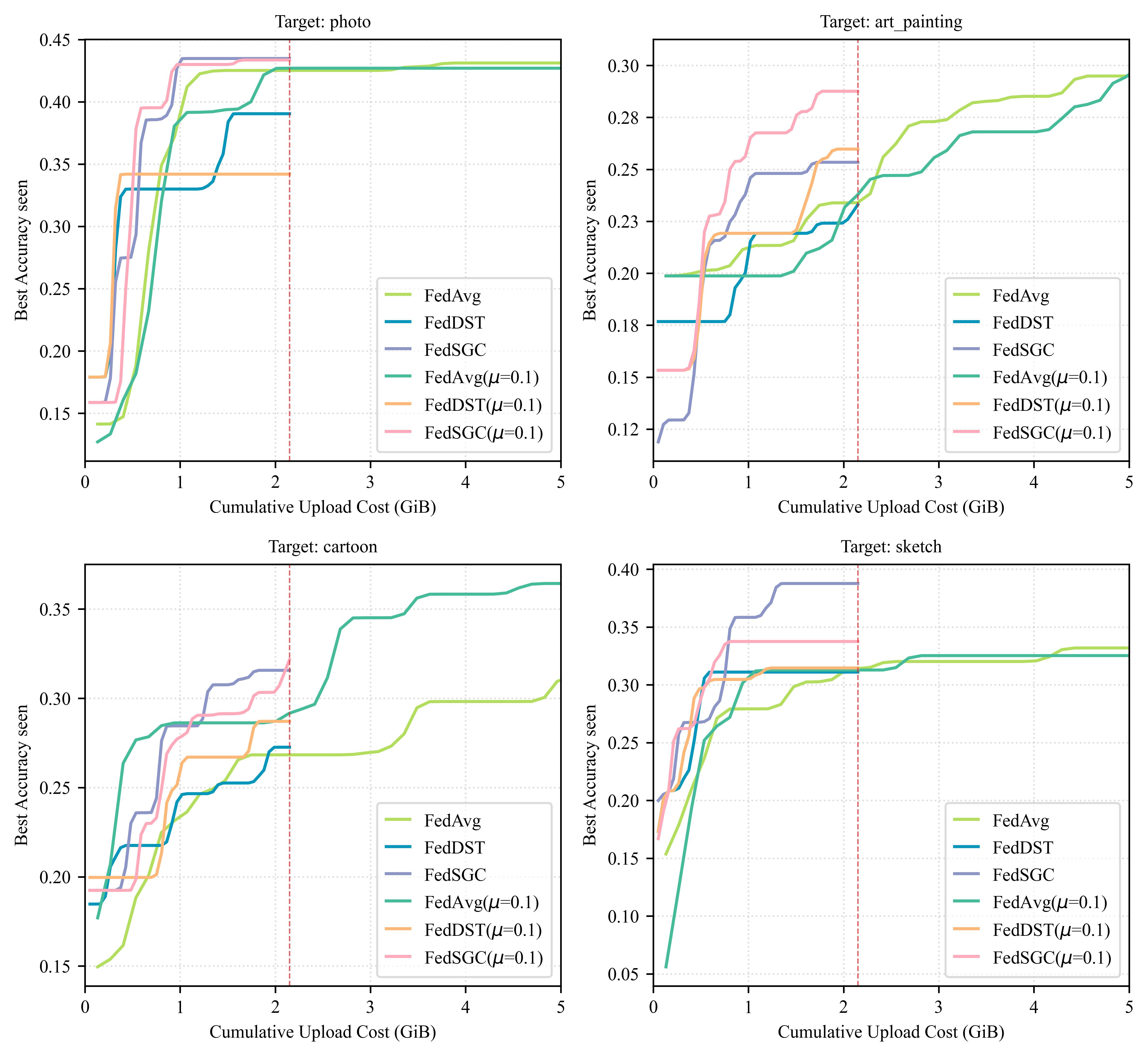
Figure 5: Results on PACS dataset.

Table 3: Accuracy of FedSGC and other baseline methods given cumulative upload bandwidth limits, on PACS dataset. We fix $S$ = 0.6 for all sparse methods, $\alpha=0.1,\Delta R=7$ for FedDST and FedSGC methods. $\lambda=0.005$ for FedSGC. We set $\mu=0.1$ for all experiments with FedProx terms. The same settings are applied for all three experiments of different target domains.

PACS	Best accuracy encountered at
	cumulative upload capacity [GiB]
Method	0.5	1.0	1.5	2.0
Photo
FedAvg	17.5	42.2	42.5	42.5
FedProx	17.5	39.2	39.4	42.7
PruneFL	16.4	26.1	30.1	33.3
GraSP	20.3	32.4	34.5	36.7
FedDST	33.0	33.0	39.0	39.0
FedDSTμ=0.1	34.2	34.2	34.2	34.2
FedSGC	27.5	43.5	43.5	43.5
FedSGCμ=0.1	39.5	43.0	43.0	43.4
Art Painting
FedAvg	20.2	21.3	21.3	23.4
FedProx	19.9	19.9	19.9	23.6
PruneFL	14.3	17.1	17.3	21.3
GraSP	15.5	16.4	18.4	24.5
FedDST	17.7	21.9	21.9	22.4
FedDSTμ=0.1	21.4	21.9	21.9	26.0
FedSGC	20.2	24.8	24.8	25.3
FedSGCμ=0.1	22.8	26.8	27.8	28.8
Cartoon
FedAvg	19.5	23.5	25.2	26.8
FedProx	27.7	28.6	28.6	28.6
PruneFL	15.6	21.5	24.3	26.4
GraSP	17.3	24.9	25.1	27.5
FedDST	21.8	24.7	25.3	27.3
FedDSTμ=0.1	20.0	26.7	26.7	28.7
FedSGC	23.6	28.5	30.8	31.6
FedSGCμ=0.1	19.2	27.9	29.1	30.3
Sketch
FedAvg	23.2	27.9	30.2	31.4
FedProx	26.4	31.3	31.3	31.3
PruneFL	22.1	25.3	29.3	30.5
GraSP	24.3	31.2	32.6	33.9
FedDST	31.1	31.1	31.1	31.1
FedDSTμ=0.1	29.7	30.5	31.5	31.5
FedSGC	26.8	35.8	38.8	38.8
FedSGCμ=0.1	30.1	33.7	33.7	33.7

Implementation. We follow the settings of previous works which also adopt PACS in federated learning experiments Nguyen et al. (2022); Zhang et al. (2023). We use ResNet-18 as the backbone, SGD with learning rate 0.001 as the optimizer for clients’ training. The target sparsity $S$ to 0.6. We iteratively pick one domain out as the target domain for global model evaluation, and make the remaining 3 domains as clients to join the federated learning process for 40 rounds, 2 epochs each round. Again, we compare all methods with the FedProx term using weight $\mu=0.1$ for all experiments, after rough tuning $\mu$ from [0.01, 0.1, 1.0].

Result Analysis. We conduct four separate experiments, each with a different domain as the target domain for testing. The full results of the four experiments are reported in Table  3, and the four line graphs showing the best accuracy achieved along the training process are presented in Figure  5. As we can see, in all experiments, FedSGC and FedSGC with FedProx term can consistently outperform the other baselines, ranking first or second. Especially in the experiment with the target domain Sketch, which is known to have the largest domain gap with the other three domains, FedSGC outperforms the other dynamic sparse training baseline, FedDST, significantly by 7.7%. We also find that the sparse training with target domains of ArtPainting and Cartoon benefits most from the FedProx term, as both FedDST and FedSGC with the prox term outperform the ones without. Surprisingly, we find that in the target-Photo and target-Sketch experiments, FedSGC can achieve even better performance using less upload capacity compared with full parameter training methods (FedAvg and FedProx). In all, our FedSGC shows greate effectiveness in realistic and challenging datasets PACS, beyond the difficulty of MNIST and CIFAR-10.

A.3 Details of Algorithm

Algorithm 1 Federated Dynamic Sparse Training

0:      Clients $[N]$ with local datasets $D_{i}$        $S=\{s_{1},\ldots,s_{l}\}$ $\to$ Sparsities by layer        $\Delta R$, $\Delta T$, $T_{end}$, $\alpha_{r}$ $\to$ Update schedule        $\mathcal{D}=\{D_{s}\}_{s=1}^{S}$ $\to$ training dataset with $C$ classes.

0:   $\mathcal{\theta^{R}},m^{R}$ $\to$ The final produced global model parameters and mask

1:  $\triangleright$ Main procedure starts

2:  Initialize server model $(\theta_{1},m_{1},d_{0})$ at sparsity $\|m_{1}\|_{0}=S,d_{1}=0$;

3:  for each round $r\in[R]$ do

4:     Sample clients $C_{r}\subset[N]$;

5:     Transmit the server model $(\theta_{r},m_{r},d_{r})$ to all clients $c\in C_{r}$;

6:     for each client $c\in C_{r}$ do in parallel do

7:        Receive $(\theta_{r}^{c},m_{r}^{c},d_{r})\leftarrow(\theta_{r},m_{r},d_{r})$ from the server;

8:        for each epoch $e\in[E]$ do

9:           $e_{c}\leftarrow e_{c}+1$

10:           Sample a mini-batch $B$ from $D_{c}$, start the training iteration $t$ on $B$;

11:           Perform one step of local training of local sparse network $\theta_{r}^{c}\odot m_{r}^{c}$;

12:           if $r\bmod\Delta R=0$ and $r<R_{end}$ and $e_{c}\bmod\Delta T=0$ and $e_{c}<T^{end}_{c}$  then

13:              Perform layer-wise magnitude pruning $(\theta_{r}^{c},m_{r}^{c})\leftarrow\text{prune}(\theta_{r}^{c};S,\sigma_{c},d_{r})$ to attain sparsity distribution $\overline{S_{c}}$ using Eq. 1 and Eq. 2;

14:              Perform layer-wise loss gradient magnitude growth $(\theta_{r}^{c},m_{r}^{c})\leftarrow\text{grow}(\theta_{r}^{c};S,\sigma_{c},d_{r})$ to restore sparsity distribution $S$ using Eq. 3 and Eq. 4;

15:           end if

16:        end for

17:        Transmit the new $(\theta_{r}^{c},m_{r}^{c})$ to the server;

18:     end for

19:     Receive the updated client-local networks and masks $(\theta_{r}^{c},m_{r}^{c})$ from clients $c\in C_{r}$;

20:     Aggregate and prune global networks to get $(\theta_{r+1},m_{r+1})$ using Eq. 5 to attain sparsity distribution $S$;

21:     Get global pseudo-gradient direction map $d_{r+1}=sign(\theta_{r+1}-\theta_{r})$ for next round training.

22:  end for

References

- Acar et al. (2021) Durmus Alp Emre Acar, Yue Zhao, Ramon Matas, Matthew Mattina, Paul Whatmough, and Venkatesh Saligrama. Federated learning based on dynamic regularization. In International Conference on Learning Representations, 2021. URL https://openreview.net/forum?id=B7v4QMR6Z9w.
- Atashgahi et al. (2022) Zahra Atashgahi, Ghada Sokar, Tim van der Lee, Elena Mocanu, Decebal Constantin Mocanu, Raymond Veldhuis, and Mykola Pechenizkiy. Quick and robust feature selection: the strength of energy-efficient sparse training for autoencoders. Machine Learning, pp. 1–38, 2022.
- Bibikar et al. (2022) Sameer Bibikar, Haris Vikalo, Zhangyang Wang, and Xiaohan Chen. Federated dynamic sparse training: Computing less, communicating less, yet learning better. In Proceedings of the AAAI Conference on Artificial Intelligence, volume 36, pp. 6080–6088, 2022.
- Chen et al. (2021) Mingzhe Chen, Nir Shlezinger, H Vincent Poor, Yonina C Eldar, and Shuguang Cui. Communication-efficient federated learning. Proceedings of the National Academy of Sciences, 118(17):e2024789118, 2021.
- Dai et al. (2023) Yutong Dai, Zeyuan Chen, Junnan Li, Shelby Heinecke, Lichao Sun, and Ran Xu. Tackling data heterogeneity in federated learning with class prototypes. In Proceedings of the AAAI Conference on Artificial Intelligence, volume 37, pp. 7314–7322, 2023.
- Evci et al. (2020) Utku Evci, Trevor Gale, Jacob Menick, Pablo Samuel Castro, and Erich Elsen. Rigging the lottery: Making all tickets winners. In International Conference on Machine Learning, pp. 2943–2952. PMLR, 2020.
- Frankle et al. (2020) Jonathan Frankle, Gintare Karolina Dziugaite, Daniel Roy, and Michael Carbin. Linear mode connectivity and the lottery ticket hypothesis. In International Conference on Machine Learning, pp. 3259–3269. PMLR, 2020.
- google (1999) google. Convolutional neural network (cnn), 1999. URL https://www.tensorflow.org/tutorials/images/cnn.
- Jiang et al. (2022) Yuang Jiang, Shiqiang Wang, Victor Valls, Bong Jun Ko, Wei-Han Lee, Kin K Leung, and Leandros Tassiulas. Model pruning enables efficient federated learning on edge devices. IEEE Transactions on Neural Networks and Learning Systems, 2022.
- Karimireddy et al. (2020) Sai Praneeth Karimireddy, Satyen Kale, Mehryar Mohri, Sashank Reddi, Sebastian Stich, and Ananda Theertha Suresh. SCAFFOLD: Stochastic controlled averaging for federated learning. In Hal Daumé III and Aarti Singh (eds.), Proceedings of the 37th International Conference on Machine Learning, volume 119 of Proceedings of Machine Learning Research, pp. 5132–5143. PMLR, 13–18 Jul 2020. URL https://proceedings.mlr.press/v119/karimireddy20a.html.
- Li et al. (2020) Ang Li, Jingwei Sun, Binghui Wang, Lin Duan, Sicheng Li, Yiran Chen, and Hai Li. Lotteryfl: Personalized and communication-efficient federated learning with lottery ticket hypothesis on non-iid datasets. arXiv preprint arXiv:2008.03371, 2020.
- Li et al. (2021a) Ang Li, Jingwei Sun, Binghui Wang, Lin Duan, Sicheng Li, Yiran Chen, and Hai Li. Lotteryfl: Empower edge intelligence with personalized and communication-efficient federated learning. In 2021 IEEE/ACM Symposium on Edge Computing (SEC), pp. 68–79. IEEE, 2021a.
- Li et al. (2021b) Qinbin Li, Bingsheng He, and Dawn Song. Model-contrastive federated learning. In Proceedings of the IEEE/CVF conference on computer vision and pattern recognition, pp. 10713–10722, 2021b.
- Liu et al. (2021) Shiwei Liu, Tianlong Chen, Zahra Atashgahi, Xiaohan Chen, Ghada Sokar, Elena Mocanu, Mykola Pechenizkiy, Zhangyang Wang, and Decebal Constantin Mocanu. Deep ensembling with no overhead for either training or testing: The all-round blessings of dynamic sparsity. arXiv preprint arXiv:2106.14568, 2021.
- Mansilla et al. (2021) Lucas Mansilla, Rodrigo Echeveste, Diego H Milone, and Enzo Ferrante. Domain generalization via gradient surgery. In Proceedings of the IEEE/CVF International Conference on Computer Vision, pp. 6630–6638, 2021.
- McMahan et al. (2017) Brendan McMahan, Eider Moore, Daniel Ramage, Seth Hampson, and Blaise Aguera y Arcas. Communication-efficient learning of deep networks from decentralized data. In AISTAT, 2017.
- Mocanu et al. (2018) Decebal Constantin Mocanu, Elena Mocanu, Peter Stone, Phuong H Nguyen, Madeleine Gibescu, and Antonio Liotta. Scalable training of artificial neural networks with adaptive sparse connectivity inspired by network science. Nature communications, 9(1):2383, 2018.
- Mostafa & Wang (2019) Hesham Mostafa and Xin Wang. Parameter efficient training of deep convolutional neural networks by dynamic sparse reparameterization, 2019. URL https://openreview.net/forum?id=S1xBioR5KX.
- Mugunthan et al. (2022) Vaikkunth Mugunthan, Eric Lin, Vignesh Gokul, Christian Lau, Lalana Kagal, and Steve Pieper. Fedltn: Federated learning for sparse and personalized lottery ticket networks. In European Conference on Computer Vision, pp. 69–85. Springer, 2022.
- Nguyen et al. (2022) A Tuan Nguyen, Philip Torr, and Ser Nam Lim. Fedsr: A simple and effective domain generalization method for federated learning. Advances in Neural Information Processing Systems, 35:38831–38843, 2022.
- Özdenizci & Legenstein (2021) Ozan Özdenizci and Robert Legenstein. Training adversarially robust sparse networks via bayesian connectivity sampling. In International Conference on Machine Learning, pp. 8314–8324. PMLR, 2021.
- Sokar et al. (2021a) Ghada Sokar, Decebal Constantin Mocanu, and Mykola Pechenizkiy. Spacenet: Make free space for continual learning. Neurocomputing, 439:1–11, 2021a.
- Sokar et al. (2021b) Ghada AZN Sokar, Elena Mocanu, Decebal Constantin Mocanu, Mykola Pechenizkiy, and Peter Stone. Dynamic sparse training for deep reinforcement learning (poster). In Sparsity in Neural Networks: Advancing Understanding and Practice 2021, 2021b.
- Tamirisa et al. (2023) Rishub Tamirisa, John Won, Chengjun Lu, Ron Arel, and Andy Zhou. Fedselect: Customized selection of parameters for fine-tuning during personalized federated learning. arXiv preprint arXiv:2306.13264, 2023.
- Tian et al. (2023) Chris Xing Tian, Haoliang Li, Yufei Wang, and Shiqi Wang. Privacy-preserving constrained domain generalization via gradient alignment. IEEE Transactions on Knowledge and Data Engineering, 2023.
- Wang et al. (2020) Chaoqi Wang, Guodong Zhang, and Roger Grosse. Picking winning tickets before training by preserving gradient flow. In International Conference on Learning Representations, 2020. URL https://openreview.net/forum?id=SkgsACVKPH.
- Wu et al. (2022) Chuhan Wu, Fangzhao Wu, Lingjuan Lyu, Yongfeng Huang, and Xing Xie. Communication-efficient federated learning via knowledge distillation. Nature communications, 13(1):2032, 2022.
- Yang et al. (2019) Qiang Yang, Yang Liu, Yong Cheng, Yan Kang, Tianjian Chen, and Han Yu. Federated learning. Synthesis Lectures on Artificial Intelligence and Machine Learning, 13(3):1–207, 2019.
- Yao et al. (2019) Xin Yao, Tianchi Huang, Rui-Xiao Zhang, Ruiyu Li, and Lifeng Sun. Federated learning with unbiased gradient aggregation and controllable meta updating. arXiv preprint arXiv:1910.08234, 2019.
- Yu et al. (2020) Tianhe Yu, Saurabh Kumar, Abhishek Gupta, Sergey Levine, Karol Hausman, and Chelsea Finn. Gradient surgery for multi-task learning. Advances in Neural Information Processing Systems, 33:5824–5836, 2020.
- Zhang et al. (2023) Ruipeng Zhang, Qinwei Xu, Jiangchao Yao, Ya Zhang, Qi Tian, and Yanfeng Wang. Federated domain generalization with generalization adjustment. In Proceedings of the IEEE/CVF Conference on Computer Vision and Pattern Recognition, pp. 3954–3963, 2023.