Interpretable Data-driven Anomaly Detection in Industrial Processes with ExIFFI

Abstract

Anomaly detection (AD) is a crucial process often required in industrial settings. Anomalies can signal underlying issues within a system, prompting further investigation. Industrial processes aim to streamline operations as much as possible, encompassing the production of the final product, making AD an essential mean to reach this goal.

Conventional anomaly detection methodologies typically classify observations as either normal or anomalous without providing insight into the reasons behind these classifications.

Consequently, in light of the emergence of Industry 5.0, a more desirable approach involves providing interpretable outcomes, enabling users to understand the rationale behind the results.

This paper presents the first industrial application of ExIFFI, a recently developed approach focused on the production of fast and efficient explanations for the Extended Isolation Forest (EIF) Anomaly detection method. ExIFFI is tested on two publicly available industrial datasets demonstrating superior effectiveness in explanations and computational efficiency with the respect to other state-of-the-art explainable AD models.

I Introduction

In recent decades, the expansion of machine learning (ML) has driven advancements in Internet of Things (IoT), particularly in the Industrial Internet of Things (IIoT). ML algorithms analyze vast datasets from interconnected sensor networks to optimize maintenance and enhance production efficiency. Unsupervised Anomaly Detection (AD) is crucial in this context, especially in settings where labeling data is impractical. Isolation Forest (IF) based models, in particular Extended Isolation Forest (EIF), stands out for its speed and performance in swiftly pinpointing anomalies [1, 2]. However, understanding anomaly causes is essential for effective resolution. Explainable Artificial Intelligence (XAI) makes ML model outputs transparent and actionable, supporting informed decision-making in IIoT environments.

This paper evaluates the recently developed Extended Isolation Forest Feature Importance (ExIFFI) algorithm, which provides a time-efficient approach to interpret the EIF model.Furthermore, a modification of EIF, named Extended Isolation Forest Plus ( $\text{EIF}^{+}$), improving generalization performances and interpretable by ExIFFI is also introduced in [3]. The algorithm’s effectiveness is showcased through its application on a real-world IIoT dataset, enhancing decision-making in industrial settings. Section II contextualizes ExIFFI within Industry 5.0, Section III explains its mechanics, and Section IV illustrates its practical applications. Section V summarizes key findings and discusses future research directions, emphasizing XAI’s role in bridging advanced ML techniques and industrial applications.

II Related Work

The shift from Industry 4.0 to Industry 5.0 emphasizes human-centric outcomes over automation and data exchange. Industry 5.0 integrates human creativity with AI and robotics, highlighting the importance of transparent and interpretable machine learning models for trust and decision-making.

Explainable Artificial Intelligence (XAI) addresses this need in industrial applications like fault detection[4], process monitoring for seminconductors [5, 6], and predictive maintenance[7]. The ExIFFI algorithm, part of the Extended Isolation Forest (EIF) model for Anomaly Detection (AD), offers fast and precise interpretation crucial for IIoT environments.

In this paper, ExIFFI is compared to various interpretation techniques, including ad-hoc methods like DIFFI[8] and post-hoc methods like KernelSHAP[9] and AcME-AD[10]. KernelSHAP provides model-agnostic interpretations at the price of being computationally intensive. On the other hand AcME-AD offers accelerated post-hoc interpretability streamlining the explanation process

Though ExIFFI and DIFFI are less flexible than post-hoc methods, they significantly boost computational speed, delivering reliable results up to 100 times faster than post-hoc modelsI. Leveraging EIF’s advanced structure, ExIFFI assesses feature significance efficiently and accurately, outperforming traditional methods[2] and avoiding the structural biases inherent in IF[11].

III Proposed Approach

ExIFFI, like DIFFI, uses the forest structure of EIF to evaluate feature significance in anomaly detection. Instead of attributing disparity to a single feature, it projects imbalance along the hyperplane’s normal vector, which represents the inclination of the cut. Given an input sample, a feature importance vector $\mathbf{I(x)}$, measuring to which extent each feature contributes to the imbalance of the considered sample is returned.

In EIF, each tree $t$ partitions the space using hyperplanes $\mathcal{H}_{k}^{t}$, defined by normal vectors $\mathbf{v}_{t}^{k}$ and intercept points $\mathbf{p}^{t}_{k}$. ExIFFI calculates feature importance by measuring imbalance at each node for a given sample $x$, noted as $\mathbf{\lambda}^{t}_{k}(\mathbf{x})$. Importance for $x$ within a tree $t$ is the sum of imbalance score of nodes $k$ traversed by $x$ to a leaf: $\mathbf{I}_{t}(x)=\sum_{k\in\mathcal{P}^{t}_{x}}\mathbf{\lambda}_{t,k}(x)$. Finally, the overall importance across the forest is obtained aggregating importance scores from trees encountering $x$: $\mathbf{I}(x)=\sum_{t\in\mathcal{T}}\mathbf{I}_{t}(x)$. In order to correct for potential biases caused by features being sampled more frequently, $\mathbf{I}(x)$ is normalized by the sum of the normal vectors composing the separating hyperplanes: $\mathbf{V}(x)$: $\mathbf{V}(x)=\sum_{t\in\mathcal{T}}\sum_{k\in\mathcal{P}^{t}_{x}}\mathbf{v}_{k}^{t}$.

Grouping these vectors yields two outputs: Global Feature Importance (GFI) and Local Feature Importance (LFI). GFI returns a single vector which associates a score to each feature, quantifying its overall importance in discriminating between inliers and outliers of the input dataset. It can be obtained as follows: $\mathbf{GFI}=\frac{\hat{\mathbf{I}}_{O}}{\hat{\mathbf{I}}_{I}}$, where $\hat{\mathbf{I}}_{O}$ and $\hat{\mathbf{I}}_{I}$ are the importance vectors computed over the set of outliers and inliers respectively. On the other hand, the Local Feature Importance ($\mathbf{LFI}$) for $x$ is calculated as: $\mathbf{LFI}(x)=\frac{\mathbf{I}(x)}{\mathbf{V}(x)}$. This metric offers a refined and normalized measure of which features significantly impact the classification of a single sample $x$ as anomalous, thereby enhancing the interpretability of anomaly detection models and facilitating targeted interventions based on the critical features identified.

IV Experimental Results

This section presents the results of applying ExIFFI to two publicly accessible datasets derived from industrial processes, which serve as benchmarks for evaluating ExIFFI’s effectiveness within real-world contexts. The datasets include Tennessee Eastman Process (TEP), which offers synthetic data with established ground truth for anomaly-inducing features [12], and Packaging Industry Anomaly DEtection (PIADE), which encapsulates typical real-world challenges such as unlabeled and high-dimensional data [13].

The outcomes discussed here were achieved using Python as the base language to implement the method and C to optimize functions embedded within the performance-critical segments of the Python code.

IV-A Industrial IoT datasets

In the following we provide an in-depth description of the structure of the benchmark datasets used in this study (i.e. TEP and PIADE) pinpointing their key characteristics and differences.

IV-A1 TEP dataset

The TEP dataset[12] is an industrial benchmark dataset containing data coming from the Tennessee Eastman (TE) process, crucial for the production of fibers, chemicals and advanced materials for everyday purpose. TEP data are obtained as the result of simulations of the TE process which can generate normal or faulty runs. Each simulation run produces a time series composed of 500 samples and 52 process variables. Each sample can be categorized into 21 classes: Class 0 denotes normal samples while Class 1-20 represent faulty instances.

Importantly prior knowledge on the features associated to the first 15 faults has been documented [14], making it possible to assess the correctness of the explanations proposed by ExIFFI and facilitates comparative analysis with alternative interpretative algorithms through the Feature Selection proxy task, as elaborated in Section IV-B.

In order to provide a better visualization of the results we consider a downsampled version of the TEP dataset. Seventy three simulations were selected: 70 normal simulations and 3 faulty ones, for a total of 35600 samples and 52 features. In particular we focus on fault type IDV12 on which domain knowledge about the most important features is available [14]. The fault considered relates to the condenser cooling water temperature and the root cause feature is xmeas_11, the separator temperature measure.

IV-A2 PIADE dataset

The Alarm logs Packaging equipment dataset (PIADE) dataset [13] is publicly available.

This dataset comprises real data produced by packaging machines. Differently from the TEP dataset, PIADE lacks of labelled data and there is no documented ground truth on the relevance of the different features used to characterize the industrial processes described. Nevertheless, it is possible to validate to correctness of the provided explanations with domain experts.

Another major difference with the respect to the TEP dataset lies in the nature of the encapsulated data. Unlike traditional IIoT datasets composed of sensor measurements, PIADE comprises statistics concerning alarm counts triggered by specific machinery, indirectly encapsulating the normal or anomalous operational states of the equipment.

PIADE contains data derived from five machines of identical type but operating under distinct conditions. Consequently, the dataset is partitioned into five sub-datasets, one for each machine. Notably, the experiments described in IV focused on the second machine (i.e. Equipment_ID equal to 2).

Finally, for what concerns the data structure, alarm logs data are aggregated into 1-hour-long time windows starting from the raw values, resulting in 2725 samples and 71 features.

IV-B Experimental Setup

To facilitate comprehension regarding the visualization of the experimental outcomes, this section will provide a description of the techniques used to evaluate and compare the different interpretability methods considered in this study.

IV-B1 Global Importance Assessment

This first experiment leverages the Global Feature Importance (GFI) score returned by ExIFFI, described in III, to rank the different attributes composing the data samples in decreasing order of relevance scores in discerning between normal and anomalous samples.

The results are depicted using a Score Plot where the first eight features in the GFI score ranking are represented by horizontal bars proportional to the importance scores.

The outcomes described in this experiment assume pivotal importance in enhancing the decision-making process which has to be performed by human operators. Indeed, the ranking obtained through GFI scores furnishes a list of the most likely causes of anomalous events in an industrial process. This knowledge can be successively harnessed by domain experts by taking preventive actions in order to avoid potential failures.

IV-B2 Local Scoremaps

Within an industrial context, where emphasis is placed on local interpretability, the Local Scoremap plot, introduced in [3], is a powerful tool in order to obtain a clear understanding of anomalous points dispersion across crucial features. This plot in fact focuses on a pair of features and its message is twofold: a scatter plot elucidates the distribution of inliers and outliers along the variables and a heatmap delineates the Local Importance scores across a grid of points within the considered two-dimensional feature space.

An important aspect for an effective usage of this visualization is the correct choice of the pair of attributes to represent. A possible strategy, as suggested in [3], is to consider the two most important features in order to visualize the distribution of anomalies along one or both axis. However, in case relevance is shared across multiple features another valid approach consists in analyzing multiple feature pairs as it is done in IV.

IV-B3 Feature Selection Proxy Task

In our final experiment, we use Feature Selection as a proxy task to assess an interpretation algorithm’s effectiveness qualitatively and quantitatively, as detailed in [3]. The premise is to start with the GFI score ranking, and if the model interpretation aligns with the ground truth, the Average Precision remains stable as irrelevant features are removed and decreases if relevant attributes are omitted. The visualization, a Feature Selection plot, shows how the Average Precision of the explained model evolves as features are incrementally discarded, both in increasing (the inverse approach) and decreasing (the direct approach) order of importance. Additionally, a random approach serves as a baseline.

It’s important to note that this analysis relies on accessible performance metrics (Average Precision score) of the explained AD model through labeled data. Thus, it was conducted solely on the TEP dataset, which has labeled anomalies.

IV-C Case Study I: TEP Dataset

In the following sections we outline the results obtained with ExIFFI on the experiments described in IV-B. In particular global and local interpretability of the $\text{EIF}^{+}$ model are assessed through the Score Plot and Local Scoremaps, presented in IV-C1 and IV-C2 respectively, and four different interpretability models are compared in IV-C3 by means of the Feature Selection Proxy Task.

IV-C1 Global Feature Importance

Figure 1 exhibits the Score Plot for the TEP dataset. Notably, two features, xmeas_22 and xmeas_11 emerge as more relevant than others. Indeed, [14] asserts that the root cause features for fault IDV12 is xmeas_11. Furthermore, saliency of xmeas_22 (i.e. the Separator cooling water outler temperature) is proven in the Sign Directed Graph included in [14]. This attribute is in fact drawn as a direct consequence of xmeas_11 in the representation. The congruity between the importance scores generated by ExIFFI and the established ground truth suggests that the causal relationship between the aforementioned attributes is plausibly leveraged by the model in the anomaly detection phase.

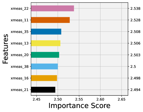
Figure 1: Global Feature Importance Score Plot TEP dataset

.

IV-C2 Local Interpretability

Figure 2 groups together the Local Scoremaps produced by ExIFFI for three distinct pairs of attributes within the TEP dataset. This presentation facilitates a comprehensive analysis of how anomalies and local importance scores vary when a significant feature such as xmeas_11 is paired with other pertinent attributes (i.e. xmeas_22 and xmeas_7) or with less salient ones (i.e. xmeas_12). In the first case, displayed in 2(b) and 2(a), anomalies (represented as red stars) exhibit a dispersed arrangement, resembling a bisector line, thereby affirming the considerable significance of both dimensions. Moreover the heatmap outlining the local importance scores partitions the feature space in two symmetric halves indicating a shared importance between the respective pairs of features. Conversely, in Figure 2(c) xmeas_11 is examined together with xmeas_12, one of the least important features in TEP, according to the GFI scores ranking. A notable distinction can be noticed in the distribution of inliers and outliers: anomalies align along the axis corresponding to feature xmeas_11, while normal points (illustrated as blue dots) are distributed along feature xmeas_12, underscoring the efficacy of this attribute in detecting normal points rather than anomalies. As a result this visualization proves the reason why these two features are correctly placed at the two opposite ends of the GFI importance ranking by ExIFFI.

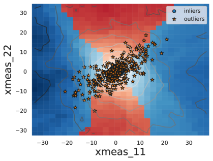
((a))

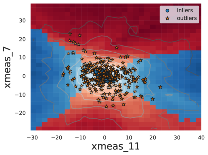
((b))

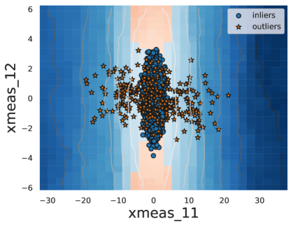
((c))

Figure 2: Local Scoremaps TEP dataset

IV-C3 Feature Selection Proxy Task

Utilizing labelled samples, a comparative analysis between various XAI models for Anomaly Detection within the TEP dataset is conducted via the Feature Selection proxy task, as elucidated in [3]. Specifically, this comparison includes two model-specific interpretation models, DIFFI [8] and ExIFFI, alongside two model-agnostic approaches: AcME-AD [10] and KernelSHAP [9]. All the models were employed to explain the predictions returned by the $\text{EIF}^{+}$ AD model, except for DIFFI, tailored specifically to provide explanations to the Isolation Forest (IF) model. As described in IV-B3 the proxy task entails the evaluation of the Global Feature Importance (GFI) score ranking of the interpretation model. However, AcME-AD and KernelSHAP algorithms primarily focus on furnishing local explanations and thus lack inherent Global Importance scores. Consequently, LFI scores of anomalous samples are used to produce the feature rankings for AcME-AD and KernelSHAP.

Figure 3 groups together the Feature Selection plots obtained for the four distinct models considered. Looking at the shape of the area enclosed between the red and blue lines and at the $AUC_{FS}$ metric values, reveals that the models showcasing the most effective explanations are ExIFFI and AcME-AD, depicted in Figure 3(d) and 3(b). Notably, the red line maintains elevated Average Precision values while the direct approach curve displays a clearer decreasing trend compared to Figures 3(a) and 3(c), resulting in higher values of $AUC_{FS}$.

Interestingly in all the aforementioned plots the red curve displays a consistent behavior for the first 30 features (i.e. 30 least important features), proving their irrelevance in influencing model performances, and a slightly declining trend in the final 5 features (i.e. 5 most important features). This distinctive pattern suggests that the TEP dataset is characterized by a cluster of relevant features sharing significance, thereby model detection performances diminishes when any attribute from this group is omitted.

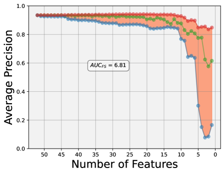
((a)) DIFFI

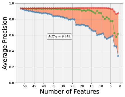
((b)) AcME-AD fitted to $\text{EIF}^{+}$

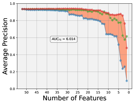
((c)) KernelSHAP fitted to $\text{EIF}^{+}$

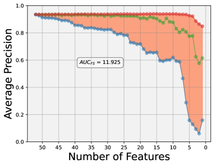
((d)) ExIFFI

Figure 3: Feature Selection plots TEP. The red, blue and green lines represent respectively the inverse, direct and random feature selection approaches.

IV-D Case Study II: PIADE Dataset

For the second case study the PIADE dataset is considered. As detailed in IV-A2 this dataset lacks of annotated samples. Consequently the application of the Feature Selection proxy task is precluded, confining the experimental results to the assessment of Global and Local interpretability, as addresses in Sections IV-D1 and IV-D2.

IV-D1 Global Feature Importance

The Score Plot displays the presence of a single feature on the top of the ranking exhibiting a substantial lead over the remaining attributes in terms of importance score: %scheduled_downtime.This variable quantifies duration of downtime resulting from scheduled maintenance operations during one hour of production time. Even without the presence of established ground truth information on the root causes of anomalies it is reasonable to infer that if several dangerous alarms are triggered, resulting in serious damages, maintenance interventions will be scheduled for packaging equipment. Among attributes related to specific alarm codes the most important ones are A_010 and A_017 whose relevance is confirmed by domain experts which identify them as known failures [15].

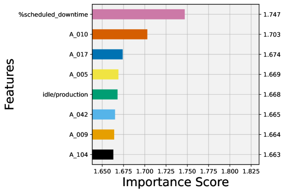
Figure 4: Global Feature Importance Score Plot PIADE dataset

.

IV-D2 Local Interpretability

Figure 5 gathers together three distinct Local Scoremaps outlining the relationship between variable %scheduled_downtime and various alarm-related features.

Figure 5(a) juxtaposes the two most important features, as delineated by the Score plot in Figure 4. The scoremap reveals a clear L-shaped distribution formed by anomalous points (i.e. red stars), perfectly aligned with features %scheduled_downtime and A_010,confirming their pivotal role in the anomaly detection task. The distinctive shape of the anomalies distribution can be interpreted as follows: during scheduled downtime phases alarms are not triggered, resulting in anomalies scattered along the horizontal axis. Conversely during production alarms, such as A_010 and A_017, are raised, as depicted by vertically aligned anomalies in both Figure 5(a) and 5(b). Among the aforementioned alarms the dispersion of outliers is more pronounced in Figure 5(a), underscoring the decisive role of A_010 in distinguishing between normal and abnormal samples.

Finally, in Figure 5(c) , %scheduled_downtime is related to the least important feature, as per the GFI score ranking produced by ExIFFI (i.e. %idle). The idle condition is the opposite operational state with respect to scheduled_downtime thus most inliers are aligned with the vertical dimension of the scoremap while the majority of the outliers are scattered along the axis representing %scheduled_downtime, as expected.

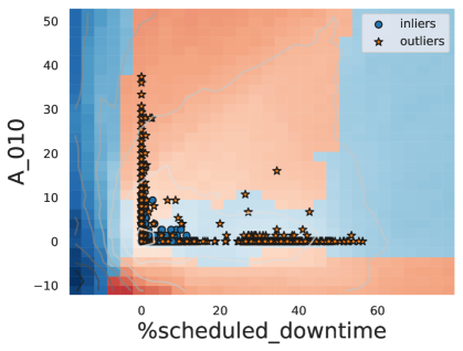
((a))

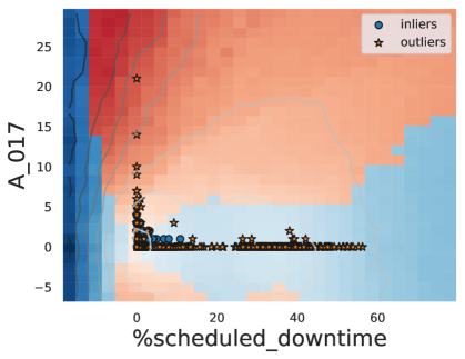
((b))

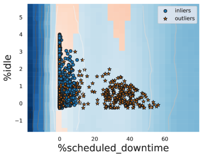
((c))

Figure 5: Local Scoremaps PIADE dataset

IV-E Time Comparison Experiment

One of the key requirements for the deployment of ML models within the context of Industrial Internet of Things is time efficiency. Given the high frequency of triggered alarms, it is indeed imperative for Anomaly Detection models to swiftly detect anomalous alarms to avoid potentially catastrophic events. Accordingly, this section focuses on comparing the computational efficiency of ExIFFI with other state-of-the-art methods: DIFFI, AcME-AD and KernelSHAP, introduced in II.

The time comparison test assesses the time taken by each one of the models under examination to generate Local Feature Importance explanation for a single anomalous point. Due to limited computational resources, KernelSHAP could only use sub-sampled version of TEP and PIADE (2% and 25% respectively) as the background data used to fit the explainer.

Table I outlines the time performances of the four models considered on both datasets. The considered algorithms fall in two classes: model-specific approaches, such as DIFFI and ExIFFI, exhibit highly efficient computational performance, capable of computing LFI scores within fractions of seconds, while model-agnostic models, AcME-AD and KernelSHAP, demonstrate significantly lower efficiency. Particularly, KernelSHAP, as outlined in II is renowned for its high computational burden, rendering it inpractical for industrial environments. Furthermore, employing sub-sampled version of the original dataset as the background leads to inaccurate explanations [16].

Comparing the computational performances of the two considered datasets, PIADE exhibits higher time values. This outcome is attributable to the elevated number of features composing this dataset, as the asymptotical complexities of KernelSHAP and AcME-AD are highly affected by the dimensionality of the dataset.

Conversely, model-specific interpretability models, DIFFI and ExIFFI, are not affected by the increased number of features in the PIADE dataset, still presenting exceptional computational efficiency. The significant speed up provided by these models, compared to AcME-AD and KernelSHAP, stems from their implementation which leverages the architecture of the high-performing IF and EIF/ $\text{EIF}^{+}$ models. In particular, EIF can be considered one of the most efficient AD models according to [2].

It is noteworthy that in both datasets ExIFFI is one order of magnitude faster than DIFFI thanks to the usage of the C programming language to optimize specific code segments. In particular, since EIF is an ensemble method, parallel computing was exploited to further speed up the computation.

	Elapsed time $\text{EIF}^{+}$ (s) TEP	Elapsed time $\text{EIF}^{+}$ (s) PIADE
ExIFFI	0.009	0.01
DIFFI	0.082	0.07
AcME-AD	4.02	7.09
KernelSHAP	112.42	138.94

TABLE I: LFI explanation times for a single sample by ExIFFI, AcME-AD, DIFFI and KernelSHAP on TEP and PIADE datasets

V Conclusions

This work demonstrates the effectiveness of our method, ExIFFI, for anomaly detection in industrial settings. It provides insightful explanations of model predictions through visualizations, aiding decision-making processes. Tested on two publicly available industrial datasets, ExIFFI accurately identified anomalies and aligned with ground truth root causes. Comparisons with state-of-the-art methods confirm its effectiveness, particularly in time efficiency for both anomaly detection and explanation. Future research directions could include the application of ExIFFI in TinyML exploiting its computational efficiency in order to empower devices with limited resources with Anomaly Detection and Root Cause Analysis capabilities.

References

- [1] F. T. Liu, K. M. Ting, and Z.-H. Zhou, “Isolation forest,” in 2008 Eighth IEEE International Conference on Data Mining, 2008, pp. 413–422.
- [2] R. Bouman, Z. Bukhsh, and T. Heskes, “Unsupervised anomaly detection algorithms on real-world data: How many do we need?” Journal of Machine Learning Research, vol. 25, no. 105, pp. 1–34, 2024. [Online]. Available: http://jmlr.org/papers/v25/23-0570.html
- [3] A. Arcudi, D. Frizzo, C. Masiero, and G. A. Susto, “Exiffi and eif+: Interpretability and enhanced generalizability to extend the extended isolation forest,” 2024.
- [4] L. C. Brito, G. A. Susto, J. N. Brito, and M. A. Duarte, “An explainable artificial intelligence approach for unsupervised fault detection and diagnosis in rotating machinery,” Mechanical Systems and Signal Processing, vol. 163, p. 108105, 2022.
- [5] M. Carletti, M. Maggipinto, A. Beghi, G. A. Susto, N. Gentner, Y. Yang, and A. Kyek, “Interpretable anomaly detection for knowledge discovery in semiconductor manufacturing,” in 2020 Winter Simulation Conference (WSC). IEEE, 2020, pp. 1875–1885.
- [6] M. Carletti, C. Masiero, A. Beghi, and G. A. Susto, “A deep learning approach for anomaly detection with industrial time series data: a refrigerators manufacturing case study,” Procedia Manufacturing, vol. 38, pp. 233–240, 2019.
- [7] S. Vollert, M. Atzmueller, and A. Theissler, “Interpretable machine learning: A brief survey from the predictive maintenance perspective,” in 2021 26th IEEE International Conference on Emerging Technologies and Factory Automation (ETFA ), 2021, pp. 01–08.
- [8] M. Carletti, M. Terzi, and G. A. Susto, “Interpretable anomaly detection with diffi: Depth-based feature importance of isolation forest,” Engineering Applications of Artificial Intelligence, vol. 119, p. 105730, 2023.
- [9] S. M. Lundberg and S.-I. Lee, “A unified approach to interpreting model predictions,” Advances in neural information processing systems, vol. 30, 2017.
- [10] V. Zaccaria, D. Dandolo, C. Masiero, and G. A. Susto, “Acme-ad: Accelerated model explanations for anomaly detection,” arXiv preprint arXiv:2403.01245, 2024.
- [11] S. Hariri, M. C. Kind, and R. J. Brunner, “Extended isolation forest,” IEEE Transactions on Knowledge and Data Engineering, vol. 33, no. 4, pp. 1479–1489, 2021.
- [12] C. A. Rieth, B. D. Amsel, R. Tran, and M. B. Cook, “Additional tennessee eastman process simulation data for anomaly detection evaluation,” Harvard Dataverse, vol. 1, p. 2017, 2017.
- [13] T. Diego, C. Enrico, C. Masiero, G. Susto, A. Beghi et al., “Packaging industry anomaly detection (piade) dataset,” 2022.
- [14] M. G. Don and F. Khan, “Dynamic process fault detection and diagnosis based on a combined approach of hidden markov and bayesian network model,” Chemical Engineering Science, vol. 201, pp. 82–96, 2019.
- [15] V. Zaccaria, C. Masiero, D. Dandolo, and G. A. Susto, “Enabling efficient and flexible interpretability of data-driven anomaly detection in industrial processes with acme-ad,” 2024.
- [16] D. Dandolo, C. Masiero, M. Carletti, D. Dalle Pezze, and G. A. Susto, “Acme—accelerated model-agnostic explanations: Fast whitening of the machine-learning black box,” Expert Systems with Applications, vol. 214, p. 119115, 2023.