Tabular and Deep Reinforcement Learning for Gittins Index

Abstract

In the realm of multi-arm bandit problems, the Gittins index policy is known to be optimal in maximizing the expected total discounted reward obtained from pulling the Markovian arms. In most realistic scenarios however, the Markovian state transition probabilities are unknown and therefore the Gittins indices cannot be computed. One can then resort to reinforcement learning (RL) algorithms that explore the state space to learn these indices while exploiting to maximize the reward collected. In this work, we propose tabular (QGI) and Deep RL (DGN) algorithms for learning the Gittins index that are based on the retirement formulation for the multi-arm bandit problem. When compared with existing RL algorithms that learn the Gittins index, our algorithms have a lower run time, require less storage space (small Q-table size in QGI and smaller replay buffer in DGN), and illustrate better empirical convergence to the Gittins index. This makes our algorithm well suited for problems with large state spaces and is a viable alternative to existing methods. As a key application, we demonstrate the use of our algorithms in minimizing the mean flowtime in a job scheduling problem when jobs are available in batches and have an unknown service time distribution.

I Introduction

Markov decision processes (MDPs) are controlled stochastic processes where a decision maker is required to control the evolution of a Markov chain over its states space by suitably choosing actions that maximize the long-term payoffs. An interesting class of MDPs are the multi-armed bandits (MAB) where given K Markov chains (each Markov chain corresponds to a bandit arm), the decision maker is confronted with a K-tuple (state of each arm) and must choose to pull or activate exactly one arm and collect a corresponding reward. The arm that is pulled undergoes a state change, while the state of the other arms remain frozen. When viewed as an MDP, the goal is to find the optimal policy for pulling the arms, that maximises the cumulative expected discounted rewards. In a seminal result, Gittins and Jones in 1974 proposed a dynamic allocation index (now known as Gittins index) for each state of an arm and showed that the policy that pulls the arm with the highest index maximizes the cumulative expected discounted rewards collected [1]. Subsequently, the MAB problem and its variants have been successfully applied in a variety of application such as $A/B$ testing, ad placements, recommendation systems, dynamic pricing, resource allocation and job scheduling [2]. Particularly for the job scheduling problem, the Gittins index policy has been shown to be optimal in minimizing the mean flow time for a fixed number of jobs. In this setting, jobs have an arbitrary service time distribution, each job corresponds to an arm and the state of each arm is the amount of service that the job has received. In fact, the Gittins index policy is known to coincide with several scheduling policies that were historically proved to be optimal under different problem settings. See [3, 4, 5] for more details. Also note that in a dynamic setting of an $M/G/1$ queue with job arrivals, the Gittins index policy has also been shown to be the optimal scheduling policy that minimizes the mean sojourn time in [6, 7]. More recently, the Gittins index policy has also been shown to minimize the mean slowdown in an $M/G/1$ queue [8]. See [1, 9, 10, 11] for various equivalent proofs on the optimality of the Gittins index policy for the MAB problem.

In a related development, Whittle in 1988 formulated the restless multi-armed bandit problem (RMAB) where the state of passive arms are allowed to undergo Markovian transitions [12]. While the Gittins index policy is no longer optimal in this setting, a similar index policy based on the Lagrangian relaxation approach was proposed, now popular as the Whittle’s index policy. The Whittle’s index policy has been observed to have near optimal performance in some problems and in fact it has been shown to be asymptotically optimal in the number of arms [13, 14]. Needless to say, the Whittle’s index policy coincides with the Gittins index when only a single arm is pulled and passive arms do no undergo Markovian transitions.

It is important to observe that the computation of Gittins or Whittle’s index requires the knowledge of the state transition probabilities for the arms. In most applications of the Gittins index policy, such transition probabilities are typically not known. One therefore has to use Reinforcement learning (RL) algorithms to learn the underlying Gittins index for different states of the arms. Duff [15] was the first to propose a Q-learning based algorithm to learn the Gittins index that uses a novel ’restart-in-state-i’ interpretation for the problem. As an application, it was shown that the algorithm could learn the optimal scheduling policy minimizing the mean flowtime for preemptive jobs appearing in batches per episode and whose service time distributions were unknown. More recently, there have been several work that propose and analyze RL algorithms for the restless multi-arm bandit case and provide tabular and deep RL algorithms. Avrachenkov and Borkar [16] were the first to propose a Q-learning based algorithm that converges to the Whittle’s index under the average cost criteria. Robledo et. al. proposed a tabular Q-learning approach called QWI in [17] and its Deep-RL counterpart QWINN in [18]. The methods proposed above make use of two timescale separations for the learning the Q-values and the Whittle’s index and are guaranteed to converge. Nakhleh et al. [19] also develop a deep reinforcement learning algorithm, NeurWIN, for estimating the Whittle indices but the paper does not provide any convergence guarantees for the underlying algorithm. Note that when passive arms do not undergo state transitions, the preceding learning algorithms (’restart-in-state’, QWI, QWINN, NeurWINN) also converge to the true Gittins index. At this point, it is not clear if there are alternative approaches for learning the Gittins index and if such approaches could be easier to implement or have better convergence properties.

In this work, we propose a tabular algorithm called QGI (Q-learning for Gittins index) and deep RL algorithm DGN (Deep Gittins network) for learning the Gittins index of states of a multi arm bandit problem. Both these algorithms are based on the retirement formulation (see [4, 11] for more detials). The DGN algorithm in particular leverages a Double DQN to learn the indices. See [20] for details on double DQN. Compared to the existing algorithms, QGI and DGN have several common as well as distinguishing features. As in case of QWI, our algorithms also have a timescale separation for learning the Q values and the indices. However, due to the nature of the retirement formulation, we are not required to learn the state-action Q values for all state action pairs but only for pairs with active (pull) action. We therefore need to learn a smaller Q-table as compared to QWI or the restart-in-state algorithm. Similarly in the DGN algorithm, we do not require experience replay tuples corresponding to the passive action (there are required in QWINN) and we use a neural network with one output (as against 2 outputs in QWINN). All these features make our algorithm not only distinct from existing ones, but offer lower runtime, better convergence and in some cases illustrate a lower empirical regret. See further sections for more details. The fact that we could use the retirement formulation to propose a new learning algorithm illustrates that there is so much more yet to investigate on this classical problem. Finally, one of our key contribution is to apply our algorithms for learning the optimal scheduling policy minimizing the mean flowtime for a fixed set of jobs with unknown service time distributions. Our results indicate that owing to the space savings offered, our algorithms are well suited for this problem and even illustrate lower empirical regret compared to other policies.

The remainder of this paper is organized as follows. Section II discusses the preliminaries on Gittins index. Whittles index and the restart in formulation. In Section III and Section IV, we propose the tabular QGI algorithm and the deep RL based DGN algorithm respectively. In these sections, we also illustrate the efficacy of our algorithms as compared to state-of-art algorithms on elementary examples. In Section V we apply the proposed algorithms to a job scheduling problem with unknown service time distributions.

II Preliminaries

II-A The Gittins index:

Consider a multi-armed bandit problem with $K$ (possibly heterogeneous) arms. Let $\mathcal{S}^{i}$ denote the state space for the $i^{th}$ arm. With slight abuse of notation, we denote the random state and action for the $i^{th}$ arm at the $n^{th}$ time step by $s_{n}(i)$ and $a_{n}(i)$, respectively where $s_{n}(i)\in\mathcal{S}^{i}$ for all $n$. Note that $a_{n}(i)=1$ if the $i^{th}$ arm is pulled at time $n$ and $a_{n}(i)=0$ otherwise. Since exactly 1 arm is pulled each time, we have $\sum_{i}a_{n}(i)=1$. Upon pulling the $i^{th}$ arm, we observe a state transition to $s_{n+1}(i)$ with probability $p(s_{n+1}(i)|s_{n}(i),a_{n}(i))$ and receive a reward $r^{i}(s_{n}(i),a_{n}(i))$. Furthermore, when $a_{n}(i)=0,$ we assume that $r^{i}(s_{n}(i),0)=0$. The objective is to choose a policy $\pi^{*}$ that maximizes the expected total discounted reward for a discount factor $\gamma$ $(0<\gamma<1$). The optimal policy is essentially a solution to the following optimization problem:

$$V_{\pi^{*}}(\bar{s})=\max_{\pi}E\left[\sum_{t=0}^{\infty}\sum_{i=1}^{K}\gamma^{t}r^{i}(s_{t}(i),a_{t}(i))\right]$$ (1)

for any starting state $\bar{s}=(s_{0}(1),\ldots,s_{0}(K))$. In a seminal work, Gittins defined the bandit allocation index in [1] which is a solution technique for the above MAB problem. In fact, the Gittins index for arm $i$ in state $x$, denoted by $G^{i}s(x)$ is given by:

$$G^{i}(x)=\sup_{\sigma>0}G^{i}(x,\sigma)=\sup_{\sigma>0}\frac{\mathbf{E}\left\{\sum_{t=0}^{\sigma-1}\gamma^{t}r^{i}(s_{t}(i),1)\mid s_{0}(i)=x\right\}}{\mathbf{E}\left\{\sum_{t=0}^{\sigma-1}\gamma^{t}\mid s_{0}(i)=x\right\}}$$ (2)

Here, $G^{i}(x,\sigma)$ is the expected discounted reward per expected unit of discounted time, when the arm is operated from initial state $x$, for a duration $\sigma$. The value $G^{i}(x)$ is the supremum of $G^{i}(x,\sigma)$ over all positive stopping times $\sigma$. In fact, it turns out that this supremum is achieved by the stopping time $\tau(x)=\min\{t:G^{i}(s_{t}(i)))<G^{i}(x)\}$, which is the time where the value of Gittins index drops from $G^{i}(x)$ for the first time while continuously pulling arm $i$. See [11] for more details.

II-B The restart-in-state formulation:

Duff was the first to propose a Q-learning based RL algorithm to learn the Gittins’ indices for the MAB problem [15]. The algorithm is based on an equivalent formulation for the MAB problem where for any fixed arm, the agent has a restart action that first teleports it to a fixed state $x$ instantaneously before moving to the next state. We henceforth call this algorithm as the restart-in-state algorithm. Since the discussion below mostly concerns a fixed arm, we drop the superscript $i$ to denote the arm for notational convenience. Instead, we denote corresponding optimal value function from starting in state $j$ by $V^{x}(j)$ (the super script $x$ now denotes the state that you will always teleport to via the restart action $0$) and is given by $V^{x}(j)=\max\left\{Q^{x}(j,1),Q^{x}(j,0)\right\}$ where

$$Q^{x}(j,1)=r(j,1)+\gamma\sum_{k}p(k|j,1)V^{x}(k)\text{~{}and~{}}Q^{x}(j,0)=r(x,1)+\gamma\sum_{k}p(k|x,1)V^{x}(k).$$

Here, $Q^{x}(j,1)$ denotes the state action value function for continuing in state $j$ while $Q^{x}(j,0)$ denotes the value corresponding to the restart action. Note that when the restart action is chosen in state $j$, there is an instantaneous transition to state $x$ at which point the action 1 is performed automatically resulting in the immediate reward of $r(x,1)$ to be earned. For some more notational convenience we will now (and occasionally from here on) denote $s_{n}(i)$ by $s_{n}$ and $r^{i}(s_{n}(i),1)$ by $r(s_{n})$, respectively. We will also suppress the action dimension, and the superscript representing arm $i$ in the reward notation when the context is clear. Given an MAB with $K$ (homogeneous) arms with $N$ states per arm, the agent pulls an arm $i$ in the $n^{th}$ step via a Boltzman distribution and observes a state transition from $s_{n}$ to $s_{n+1}$ and receives a reward $r(s_{n})$. For learning the Gittins index using a Q learning approach, this single transition is utilised to do two updates for each $k\in\mathcal{S}$. The first update corresponds to taking the action ‘continue’ in state $s_{n}$ and transitioning to state $s_{n+1}$ for all restart in $k$ problems. The second update corresponds to choosing to teleport to $s_{n}$ from any state $k$ and then observing the transition to $s_{n+1}$. A single reward $r(s_{n})$ leads to the following $2N$ Q-learning updates where for each $k\in\mathcal{S}$ we perform:

$$Q_{n+1}^{k}(s_{n},1)=(1-\alpha(n))Q_{n}^{k}(s_{n},1)+\alpha(n)\left[r(s_{n})+\gamma\max_{a\in\{0,1\}}Q_{n}^{k}(s_{n+1},a)\right]$$ (3)

$$Q_{n+1}^{s_{n}}(k,0)=(1-\alpha(n))Q_{n}^{s_{n}}(k,0)+\alpha(n)\left[r(s_{n})+\gamma\max_{a\in\{0,1\}}Q_{n}^{s_{n}}(s_{n+1},a)\right].$$ (4)

Here, $\alpha(n)$ is the learning rate and the Gittins index for a state $x$ is tracked by the $Q_{n}^{x}(x,1)$ value. In writing the preceeding two equations, we are assuming that the arms are homogeneous and therefore the same Q-values can be updated, irrespective of the arm chosen. For a more general setting where the arms can be heterogeneous, we need to have a separate Q-table for each arm. Needless to say, the time complexity for each iteration is $O(2N+N)$ and space complexity is $O(2\cdot N^{2}\cdot K)$. See [15] for more details.

II-C A Whittle index approach to learn Gittins index:

The Whittles index is a heuristic policy introduced in [12] for the restless multi-arm bandit problem (RMAB). Here, $M$ out of $K$ arms must be pulled and the passive arms (arms that are not pulled) are allowed to undergo state transitions. For the setting where state transitions probabilities are unknown (for both active and passive arms), RL based methods (QWI, QWINN) to learn the Whittle indices have recently been proposed [17, 18]. When the passive arms do not undergo state transitions, the Whittle index coincides with the Gittins index and therefore these algorithms can in fact be used to learn the underlying Gittins index. Using the notion of a reference state $x$ (see [17] for details), the corresponding Q-learning based update equations for learning the Gittins index are as follows:

$$Q_{n+1}^{x}\left(s_{n},a_{n}\right)=(1-\alpha(n))Q_{n}^{x}\left(s_{n},a_{n}\right)+\alpha(n)\left(\left(1-a_{n}\right)\left(\lambda_{n}(x)\right)+a_{n}r\left(s_{n}\right)+\gamma\max_{v\in\{0,1\}}Q_{n}^{x}\left(s_{n+1},v\right)\right)$$ (5)

$$\lambda_{n+1}(x)=\lambda_{n}(x)+\beta(n)\left(Q_{n}^{x}(x,1)-Q_{n}^{x}(x,0)\right).$$ (6)

Here, $\lambda_{n}(x)$ denotes the Whittles index for state $x$ and $r(s_{n})$ denotes the reward for pulling an arm in state $s_{n}$, in the $n^{th}$ step. As earlier, the dependence on arm $i$ is suppressed in the notation.

III QGI: Q learning for Gittins index

In this section, we present a Q-learning based algorithm for learning the Gittins index (QGI for short) that is based on the retirement formulation proposed by Whittle [21]. We first recall the retirement formulation for ease of exposition.
The retirement formulation: First assume you have a single arm that is in state $x$. For this arm, you can either pull the arm and collect reward or choose to retire and receive a terminal reward $M$. Let us denote the optimal value function in state $x$ by $V_{r}(x,M)$. The actions are denoted by $1$ (to continue) and $0$ (to retire). The Bellman optimality equation for this problem is:

$$V_{r}(x,M)=max\{Q_{M}(x,1),Q_{M}(x,0)\}$$

where $Q_{M}(x,1)=r(x,1)+\gamma\sum_{j}p(j|x,1)max\{Q_{M}(j,1),Q_{M}(j,0)\}$ and $Q_{M}(x,0)=M$. As shown in [21], this results in an optimal stopping problem (how long should you choose action 1 before retiring) and the Gittins index for state $x$ is given by $G(x)=M(x)(1-\gamma)$ where

$$M(x)=inf\{M:V_{r}(x,M)=M\}.$$ (7)

Clearly, $G(x)$ can be obtained by finding the smallest value of $M$ where $V_{r}(x,M)=M$. It is important to note here that $V_{r}(x,M)$ is bounded, convex and non-decreasing in $M$ [11, 21].

III-A The tabular QGI algorithm

Now suppose that state $x$ is fixed as a reference state and the retirement amount is set to $M(x)$ which is proportional to the Gittins index for state $x$. In that case, the Bellman equations are

$$V_{r}(x,M(x))=max\{Q_{M(x)}(x,1),Q_{M(x)}(x,0)\}\text{~{}where~{}}$$

$$Q_{M(x)}(x,1) = r(x,1)+\gamma\sum_{j}p(j|x,1)max\{Q_{M(x)}(j,1),Q_{M(x)}(j,0)\}$$

$$Q_{M(x)}(j,1) = r(j,1)+\gamma\sum_{k}p(k|j,1)max\{Q_{M(x)}(k,1),Q_{M(x)}(k,0)\}\text{~{}and~{}}$$

$$Q_{M(x)}(j,0) = M(x)\text{~{}for all $j$~{}}.$$

Now in a setting where the transitions probabilities are unknown, our goal is to learn the Gittins index for each state in all arms. For simplicity lets assume homogeneous arms and consider one such arm. For this arm, our aim is to learn the indices $M(x)$ for every $x\in\mathcal{S}$. Note that in the Bellman equations above, $x$ plays the role of a reference state and to come up with appropriate Q learning equations, we need an additional dimension in the Q-table for the reference state. This is similar in spirit with the requirement for the reference state in Eq. (5). Also note that since $M(x)=Q_{M(x)}(j,0)$ for all $j$ in the Belleman equations above, we can have an iterative update equation for $M(x)$ and completely ignore the entries corresponding to $Q_{M(x)}(j,0)$from the Q -table.

For a K-armed bandit in state $(s_{n}(0),s_{n}(1),...s_{n}(K))$ in the $n^{th}$ step, the agent selects an arm via an $\epsilon$-greedy policy based on the current estimates of indices, denoted by $(M_{n}^{0}(s_{n}(0)),\ldots,M_{n}^{K}(s_{n}(K))$. Upon pulling an arm, say $i$, the agent observes a transition from state $s_{n}(i)$ to $s_{n+1}(i)$, and a reward $r^{i}\left(s_{n}(i)\right)$. As earlier, since arms are homogeneous, we will denote $s_{n}(i)$ by $s_{n}$, $M_{n}^{i}(s_{n}(i))$ by $M_{n}(s_{n})$ and $r^{i}\left(s_{n}(i)\right)$ by $r(s_{n})$. This reward $r(s_{n})$ can be used to update the Q values for $s_{n}$ for each reference state leading to $N$ Q-learning updates. This is followed with pushing current estimate of $M(\cdot)$ in direction of $V_{r}(\cdot,M)$, motivated by equation (7). This gives rise to the following pair of update steps in the chosen arm upon observing each transition. For each reference state $x\in\mathcal{S}$, when an arm in state $s_{n}$ is pulled, we perform:

$$Q_{n+1}^{x}\left(s_{n},1\right)=Q_{n}^{x}\left(s_{n},1\right)+\alpha(n)\left(r\left(s_{n}\right)+\gamma\max\left\{Q_{n}^{x}(s_{n+1},1),M_{n}(x)\right\}-Q_{n}^{x}\left(s_{n},1\right)\right)$$ (8)

and

$$M_{n+1}(x)=M_{n}(x)+\beta(n)\left(\max\left\{Q_{n+1}^{x}(x,1),M_{n}(x)\right\}-M_{n}(x)\right).$$ (9)

For ease of exposition, we have assumed here that all arms are homogeneous and therefore in the above equations, the same Q-table entries are updated for different arms visiting the same state. It is also important to note that we have not used $Q_{n}^{x}(s_{n+1},0)$ to bootstrap and so we need not update those values. In fact, we do not even need to store them. For a guaranteed convergence to the true Gittins indices (see Theorem 1), the learning rate sequence $\alpha(n)$ and $\beta(n)$ are chosen to satisfy $\sum_{n}\alpha(n)=\infty,\sum_{n}\alpha(n)^{2}<\infty$, $\sum_{n}\beta(n)=\infty,\sum_{n}\beta(n)^{2}<\infty$. We also require that $\beta(n)=o(\alpha(n))$ that allows for two distinct time scales, namely, a relatively faster time scale for the updates of the state-action function, and a slow one for the Gittins indices. At this point, it would be a good idea to compare and contrast our learning equations with that of QWI and restart-in-state algorithm which are recalled here for convenience.

$$Q_{n+1}^{x}\left(s_{n},a_{n}\right)=(1-\alpha(n))Q_{n+1}^{x}(s_{n},a_{n})+\alpha(n)\left(\left(1-a_{n}\right)\left(\lambda_{n}(x)\right)+a_{n}r_{1}\left(s_{n}\right)+\gamma\max_{v\in\{0,1\}}Q_{n}^{x}\left(s_{n+1},v\right)\right)$$ (10)

$$\lambda_{n+1}(x)=\lambda_{n}(x)+\beta(n)\left(Q_{n}^{x}(x,1)-Q_{n}^{x}(x,0)\right)$$ (11)

$$Q^{k}(s_{n},1)=(1-\alpha(n))Q^{k}(s_{n},1)+\alpha(n)\left[r(s_{n})+\gamma\max_{a\in\{0,1\}}Q^{k}(s_{n+1},a)\right]$$ (12)

It is quite evident that the update equations (10), (12) are performed for both actions $a_{n}=1$ and $a_{n}=0$ and in fact $Q_{n}^{x}\left(x,0\right)$ is also directly involved in the update of the Gittins indices (see equation (11)). In contrast, there is no Q-value term corresponding to retirement action in both equations (8) and (9). We only consider $a_{n}=1$ for the Q-table, reducing its size by a factor of 2. Let us now carefully observe Eq. (9). We see that $V_{r,n}(x,M_{n}(x))=\max\left(Q_{n}^{x}(x,1),M_{n}(x)\right)$ is being invoked to push $M_{n}(x)$ in its direction. Let us recall that $V_{r}(x,M)$ is bounded, non-increasing and convex w.r.t $M$. Hence, one of two following cases arise. Either, $M$ is large and hence it dominates, making $V_{r}(x,M)-M=0$, in which case (9) is not updated. It is only if $Q_{n}^{x}(x,1)>M_{n}(x)$, $M_{n}(x)$ is updated in Eq. (9). Therefore, in Eq. (9), $M_{n}(x)$ needs to initialised by a value which is known to be smaller than the Gittins index in that state. To avoid imposing this restriction, we simply replace $V_{r,n}(x,M)$ by $Q_{n}^{x}(x,1)$, and this allows us to initialise $M$ to arbitrary value. We therefore use the following equation in QGI in place of Eq. (9):

$$M_{n+1}(x)=M_{n}(x)+\beta(n)\left(Q_{n+1}^{x}(x,1)-M_{n}(x)\right).$$ (13)

Algorithm 1 QGI for N states, K arm bandits

0:  Discount parameter $\gamma\in(0,1)$, exploration parameter $\epsilon\in[0,1]$

1:  Initialise M (NxK) and Q (NxNxK) matrix for all states in each arm

2:  Initialize $s_{0}$ for all arms

3:  for $n=1$ to $n_{\text{end}}$ do

4:     Select an arm $i$ to pull through $\epsilon$-greedy policy

5:     Get new state $s_{n+1}(i)$ and reward $r(s_{n}(i))$ from state $s_{n}(i)$

6:     Update learning rate $\alpha(n)$, $\beta(n)$

7:     Update $Q^{x}_{n}(s_{n}(i),1)$ for all $x\in\mathcal{S}$ via (8)

8:     Update $M_{n}(x)$ for all $x\in\mathcal{S}$ via (13)

9:  end for

We are now in a position to present the QGI algorithm (Algorithm 1) that essentially makes use of Eq. (8) and (13). Let $N:=|\mathcal{S}|$ denote the number of states of an arm. For a fixed $\epsilon$ and $\gamma$, we arbitrarily initialise the initial states of the K arms. We then initialize a $Q$ matrix of size $N\times N\times K$ and a vector $M$ of size $N\times 1$. If the arms are homogeneous, then the Q table has a size of $N\times N$. We then choose the best arm (arm with the highest estimate of Gittins index) with a probability of $1-\epsilon$, and choose an arm randomly with probability $\epsilon$. In the chosen arm $i$, we observe a state transition from $s_{n}$ to $s_{n+1}$ with a reward $r\left(s_{n}\right)$. We use this to update our Q-values and $M$ vector as in Eq. (8) and (13). Our algorithm uses two timescales for updating $Q$ and $M$ where the updates for $M$ are on a slower timescale. Timescale separation is indicated by the use of different learning rates $\alpha(n)$ and $\beta(n)$ in Algorithm 1. Owing to the nature of updates presented in Eq. (8) and (13), while the time complexity in QWI and the restart-in formulation per iteration is the same, we have the following two-fold advantage leading to lower runtime and apparent smoother convergence (see numerical results):

• The effective updates in each iteration to the Gittins index values are $N$, compared to just $1$ in restart-in-state. We have observed that this leads to better convergence of the Gittins index values (see Section V). In QWI, $NK$ updates are done to Q values and $N$ updates to $\lambda$ in each iteration when $\beta\neq 0$. Out of those $NK$ updates, $N(K-1)$ updates are done to $Q^{x}(s_{n},0)$ for all arm and for all $x$ and only $N$ updates to the values corresponding to $a_{n}=1$. In contrast, QGI does $N$ updates only to $Q^{x}(s_{n},1)$ for all $x$ as Q-values for $a_{n}=0$ is neither stored nor updated.

• Since, since $Q_{n}^{x}(s_{n+1},0)=M_{n}(x)$ for all $s_{n},$ we do not track and update values of $Q_{n}^{x}(s_{n},0)$ for every $x$ and $s_{n}$ resulting in significant space saving. In restart-in-state and QWI, the size of Q-table for each arm is $N\times N\times 2$. Here the first $N$ corresponds to all reference states, the second $N$ corresponds to all states and $2$ for the actions of continue or stop. On the other hand, in QGI the Q-table for each arm is of the size $N\times N$.

The space saving discussed above is significant when the number of states or arms are very large. For example, for a 10 armed bandit with 100 states, we can observe that the Q-table will have $2,00,000$ entries for the restart-in-state algorithm, 2,01,000 entries for QWI while only 1,01,000 entries in QGI. We find this as a very useful feature, particularly for learning the optimal scheduling policy minimizing mean flowtime for a fixed number of jobs having arbitrary but continuous service time distributions. See Section V-B for details.

Before we move on to the numerical comparisons, we state the following theorem that guarantees convergence of the Gittins index using the QGI algorithm. Proof is based on the convergence analysis of stochastic approximation based recursions with two timescales and follows along similar lines to the convergence of QWI [18]. A proof outline is given in the appendix for completeness.

Theorem 1.

Given learning rate sequences $\alpha(n)$ and $\beta(n)$ such that $\sum_{n}\alpha(n)=\infty,\sum_{n}\alpha(n)^{2}<\infty$, $\sum_{n}\beta(n)=\infty,\sum_{n}\beta(n)^{2}<\infty$ and $\beta(n)=o(\alpha(n))$, iterative equations (8) and (13) converge to the optimal state-action values for the Gittins index policy $Q_{G}(s,a)$, and to the Gittins indices $G(s)=(1-\gamma)M(s)$, where $M_{n}(s)\rightarrow M(s)$ and $Q_{n}(s,a)\rightarrow Q_{G}(s,a)$ for all $s\in S$, $a\in A$ as $n\rightarrow\infty$.

III-B Elementary example

We now illustrate the efficacy of the QGI algorithm on a slightly modified version of the restart problem from [18]. The problem was modified to work for rested bandits (passive arms do not undergo state transitions). Here, the state space $S=\left\{0,1,2\right\}$ and there are 2 homogeneous arms. The transition probability matrix in the case of active action is:

$$P(s^{\prime}|s,1)=\begin{bmatrix}0.1&0.9&0\\ 0.1&0&0.9\\ 0.1&0&0.9\\ \end{bmatrix}$$

The reward for pulling an arm in state $s$ is given by $r(s)=0.9^{s}+1$. The Gittins index can be analytically calculated in this problem, yielding G(0) = 0.9, G(1) = 0.814, G(2) = 0.758 while using a discount factor $\gamma$ = 0.9, see [22]. We note that the Gittins index is decreasing as the state increases which is consistent with the reward structure. We experimented with learning rates of same order, $\alpha(n)=0.3$ and $\beta(n)=0.2$. In this case the $\epsilon$ was set to $0.4$ for QGI. For QWI, we choose $\epsilon=1$ as mentioned in [18]. We ran all three algorithms for this experiment and the respective indices are shown in Fig. 1. Clearly, the QGI algorithm converges quickly compared to the restart-in-state algorithm to the true index value and is also less noisy as compared with QWI.

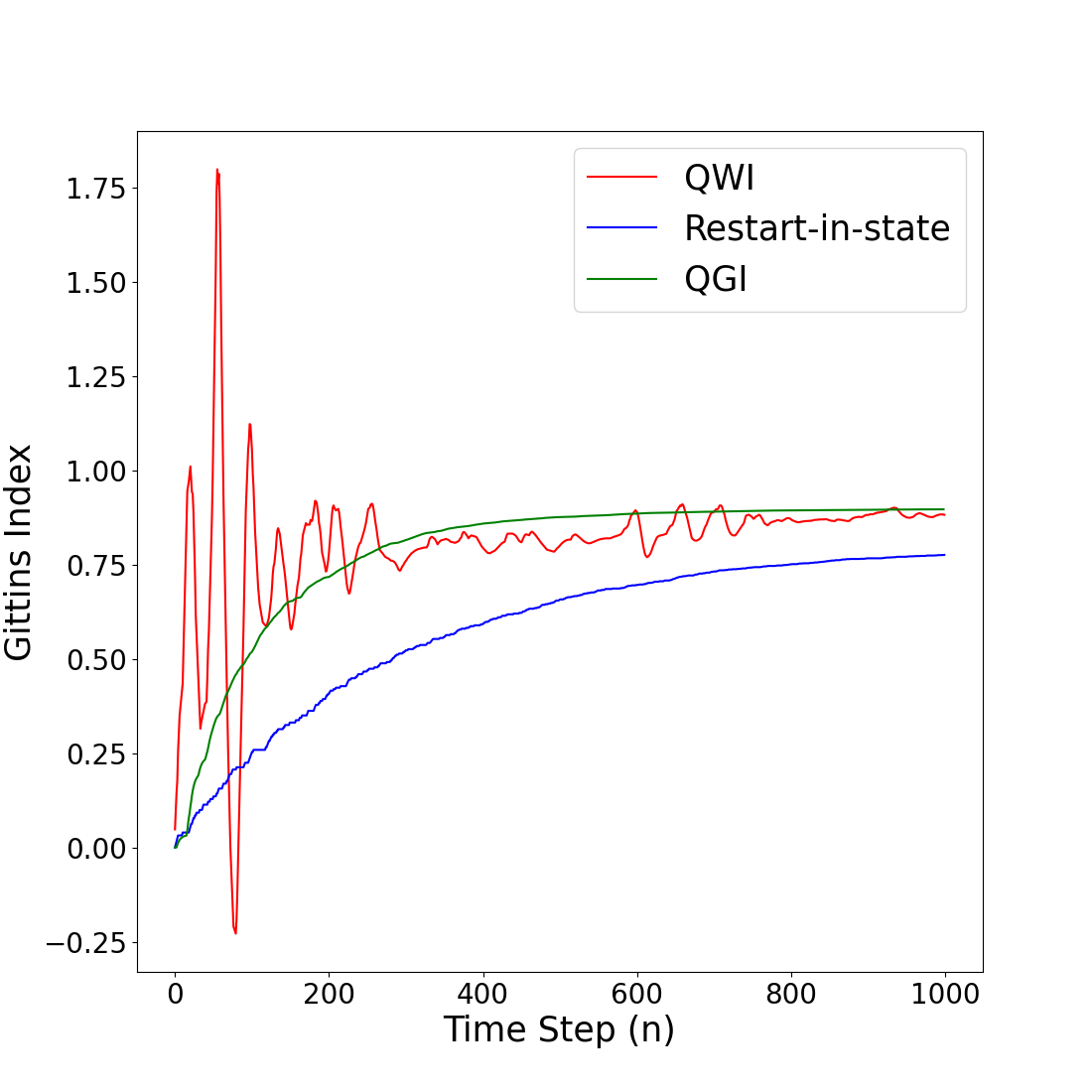
(a) State 0

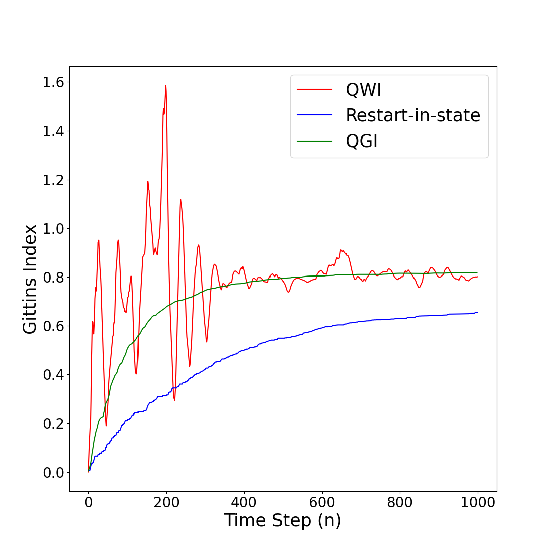
(b) State 1

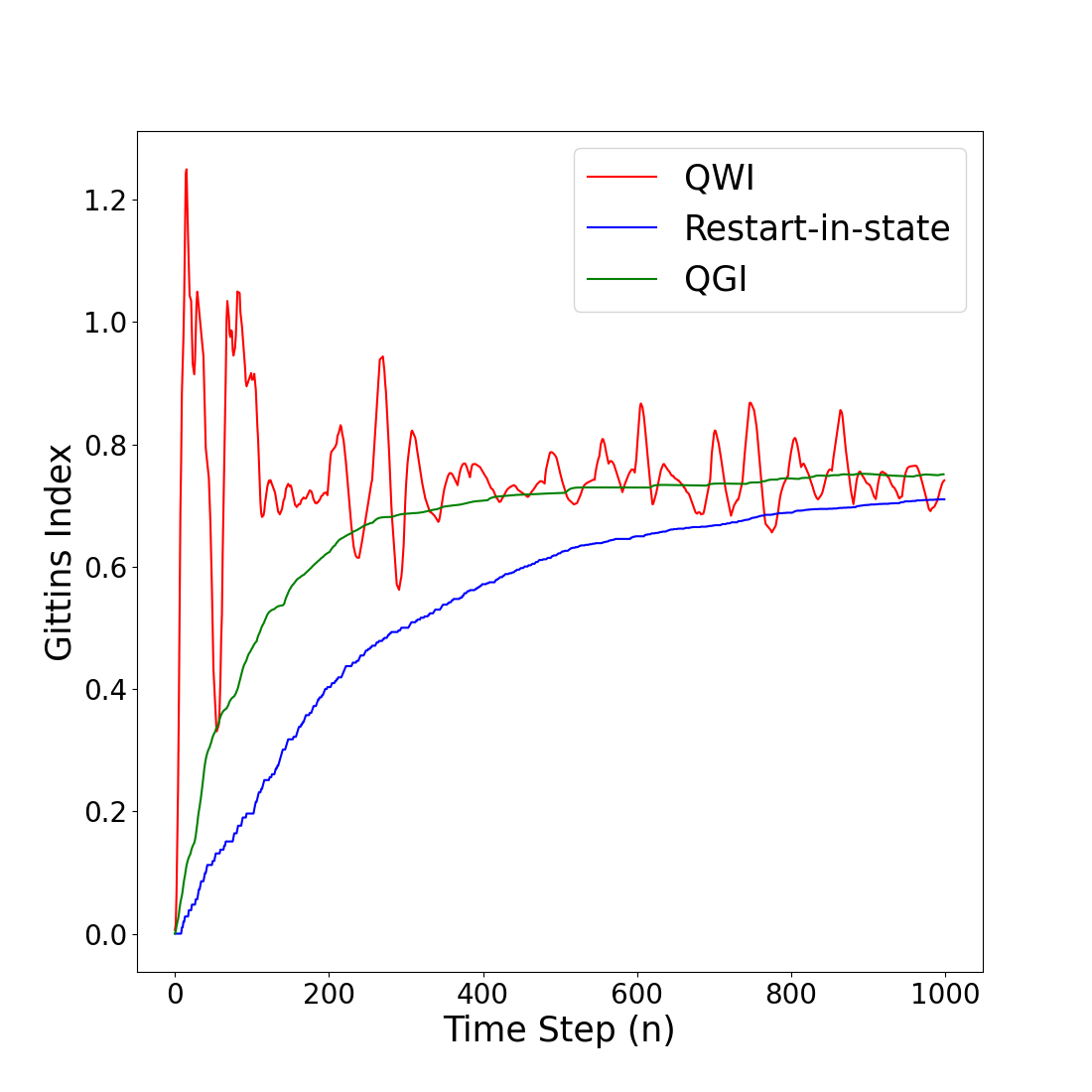
(c) State 2

Figure 1: (a), (b) and (c) compares the convergence of Gittins Indices for QGI, QWI and the restart-in-state algorithm.

IV DGN: Deep Gittins Network

The DGN (Deep Gittins Network) algorithm is based on learning the Gittins estimates through a neural network instead of the tabular method of QGI. Note that DGN is also based on the the retirement formulation and much of the discussion leading up to Equations (8) and (13) is also relevant to this deep-RL formulation. We use a neural network with parameters $\theta$ as a function approximator for the state action value function $Q^{x}(s,1)$. The input to the neural network is the current state $s_{n}$ and reference state $x$ and the output represents $Q_{\theta}^{x}(s,1)$. As noted in the tabular method QGI, we are not required to approximate the stat-action value function $Q^{x}(s,0)$ corresponding to the retire option. As in QGI, since $Q^{x}(s,0)$ is equal to the retirement value $M(x)$, we use a separate stochastic approximation equation to track the Gittins index $M(x)$ in state $x$.

The fact that our neural network has only one output corresponding to $Q_{\theta}^{x}(s,1)$, reduces the overall complexity of the network. This is unlike the QWINN algorithm where the neural networks have two outputs corresponding to both actions, and approximating both outputs accurately seems computationally more expensive. Our DGN algorithm utilises a Double-DQN architecture for better convergence guarantee [20]. Therefore a second (target) neural network with parameters $\theta^{\prime}$ is used to calculate the target Q-values by bootstrapping with our current estimate. These are denoted by $Q_{\theta^{\prime}}^{x}\left(s_{n+1},1\right)$. To further improve stability and reduce variance in target estimates, we do a soft update to $\theta^{\prime}$ values instead of copying the $\theta$ values directly to the target network [23]. The soft updating for $\theta^{\prime}$ is done using the iteration $\theta^{\prime}=\tau\theta^{\prime}+\left(1-\tau\right)\theta$, once in every $\kappa$ number of steps.

As in QGI, the agent starts by pulling an arm $i$ in state $s_{n}(i)$ via an $\epsilon$-greedy policy based on the current estimate of Gittins indices. This results in a transition to state $s_{n+1}(i)$ and a reward $r^{i}(s_{n}(i))$ is observed. The observed state transitons and rewards are appended with the reference state $x$ to form an experience tuple that is denoted by $(x,s_{n}(i),a_{n}(i),r^{i}(s_{n}(i)),s_{n}(i+1),M_{n}(x))$. In fact, we create $N$ different tuples by considering every reference state $x\in\mathcal{S}$. Each state transition is therefore used to update the Q-values for all reference states $x$, and to generate $N$ tuples as mentioned above. These tuples are stored along with other tuples in what is called as a replay buffer. Note that since we are in the Gittins setting, there are no rewards from passive action and therefore we do not create experience tuples corresponding to action $a_{n}=0$. This results in a replay buffer with a smaller size as compared with the replay buffer of QWINN where experience tuples corresponding to action 0 are stored as well. After collecting enough experience tuples, we randomly create a minibatch of size $B$ to iterate upon. For each experience tuple in a minibatch, we first pass the pair $(s_{n}(i),x)$ through the primary network to get $Q_{\theta}^{x}(s_{n}(i),1)$ for all $x\epsilon\mathcal{S}$. Then the pairs $(s_{n+1}(i),x)$ are fed to the target network to get $Q_{\theta^{\prime}}^{x}\left(s_{n+1}(i),1\right)$ values. This allows us to compute $Q_{\text{target }}^{x}\left(s_{n}(i),1\right)$ values as following:

$$Q_{\text{target }}^{x}\left(s_{n}(i),1\right)=r\left(s_{n}(i)\right)+\gamma\max\left(Q_{\theta^{\prime}}^{x}\left(s_{n+1}(i),1\right),M_{\theta^{\prime}}(x)\right)$$ (14)

Once we have calculated the $Q_{\text{target }}^{x}\left(\cdot\right)$ and $Q_{\theta}^{x}(\cdot)$ values for the minibatch, we calculate the mean-squared loss as follows:

$$\text{Mean Squared Loss}=\frac{1}{B}\sum_{i=1}^{B}\sum_{x=1}^{N}(Q_{\text{target}}^{x}(s(i),1)-Q_{\theta}^{x}(s(i),1))^{2}$$

Then we update the $\theta$ values in the neural network via an appropriate optimizer (we use the Adam optimiser for our numerical results). In our implementation, we collect experience tuples and add them to the replay buffer in every step but do the parameter update steps along with the soft update once in every $\kappa=10$ steps. This is coupled with the stochastic approximation update for $M$ as follows:

$$M_{n+1}(x)=M_{n}(x)+\beta(n)\left(Q_{\theta}^{x}(x,1)-M_{n}(x)\right).$$ (15)

We repeat the process for each sampled minibatch until convergence of the Gittins estimates. The neural network in our experiment consists of three hidden layers with (64,128,64) neurons. For the activation function, ReLU is used. This algorithm is formulated as shown in Algorithm 2.

Algorithm 2 DGN Algorithm

1:  Input: Discount parameter $\gamma\in(0,1)$, exploration parameter $\epsilon\in[0,1]$, Learning rate, minibatch size $B$, Soft update parameter $\tau\in[0,1]$ and $\kappa=10$.

2:  Output: Gittins index vector for all states

3:  Initialize $s_{0}(\cdot)$ for all arms

4:  for $n=1$ to $n_{\text{end}}$ do

5:     Pull an arm $i$ through $\epsilon$-greedy policy

6:     Do a transition from state $s_{n}(i)$ to $s_{n+1}(i)$ and observe reward $r(s_{n}(i))$

7:     Save each arm’s experience replay tuple into separated replay buffers

8:     if size of replay buffer $>$ threshold $\&$ $(n$ modulo $\kappa$ $==0)$ then

9:        $\beta(n)$

10:        Sample a minibatch of size B

11:        for $x\in S$ do

12:           Predict $Q_{\theta}^{x}(s_{n}(i),1)$ values for each sample

13:           Compute target $Q_{\text{target }}^{x}\left(s_{n}(i),1\right)$ for each sample as in Eq. (14)

14:        end for

15:        Compute MSE loss between $Q_{\theta}$ and $Q_{\text{target}}$

16:        Update the $\theta$ parameters through backpropagation

17:        Update target parameters as $\theta^{\prime}=\tau\theta^{\prime}+\left(1-\tau\right)\theta$

18:     end if

19:     Update M (Retirement reward) via (15)

20:  end for

IV-A Elementary example

Now let us consider the problem discussed in 3.2 and draw a emperical comparison between DGN and QWINN. For the experiment, we fixed the following hyperparameters: $\gamma=0.9$, $B=32$, $\tau=1e-3$, $\kappa=10$ and $\beta(n)=0.7\times 1_{\{n~{}modulo~{}20\equiv 0\}}$. Initial value of $\epsilon$ was kept as 1 and its decay was scheduled as $\epsilon_{n+1}=max(\epsilon_{n}\times 0.9995,0.1)$. The numerical results are as shown in Fig. 2. A clear benefit of using DGN over QWINN seems ot be that the indices converge more smoothly to the desired values.

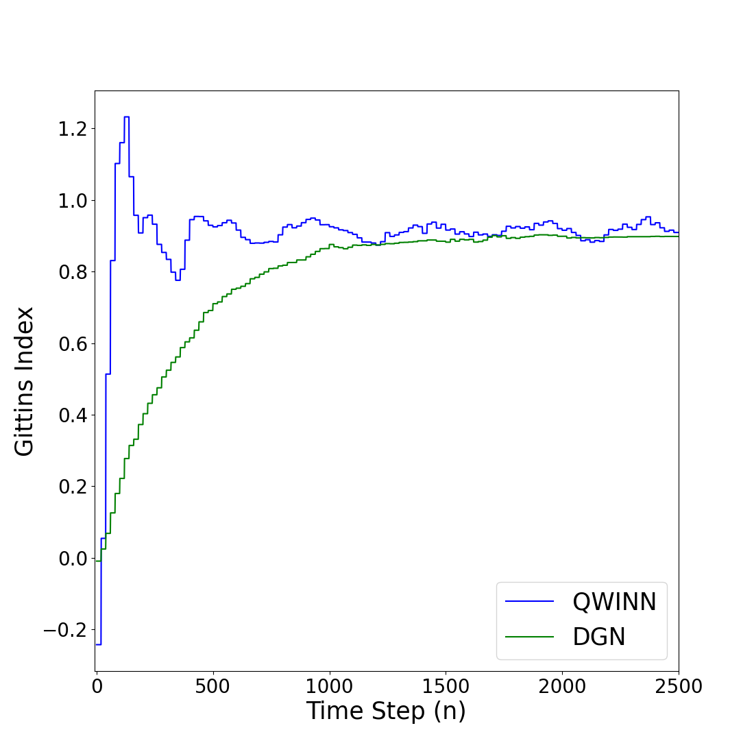
(a) State 0

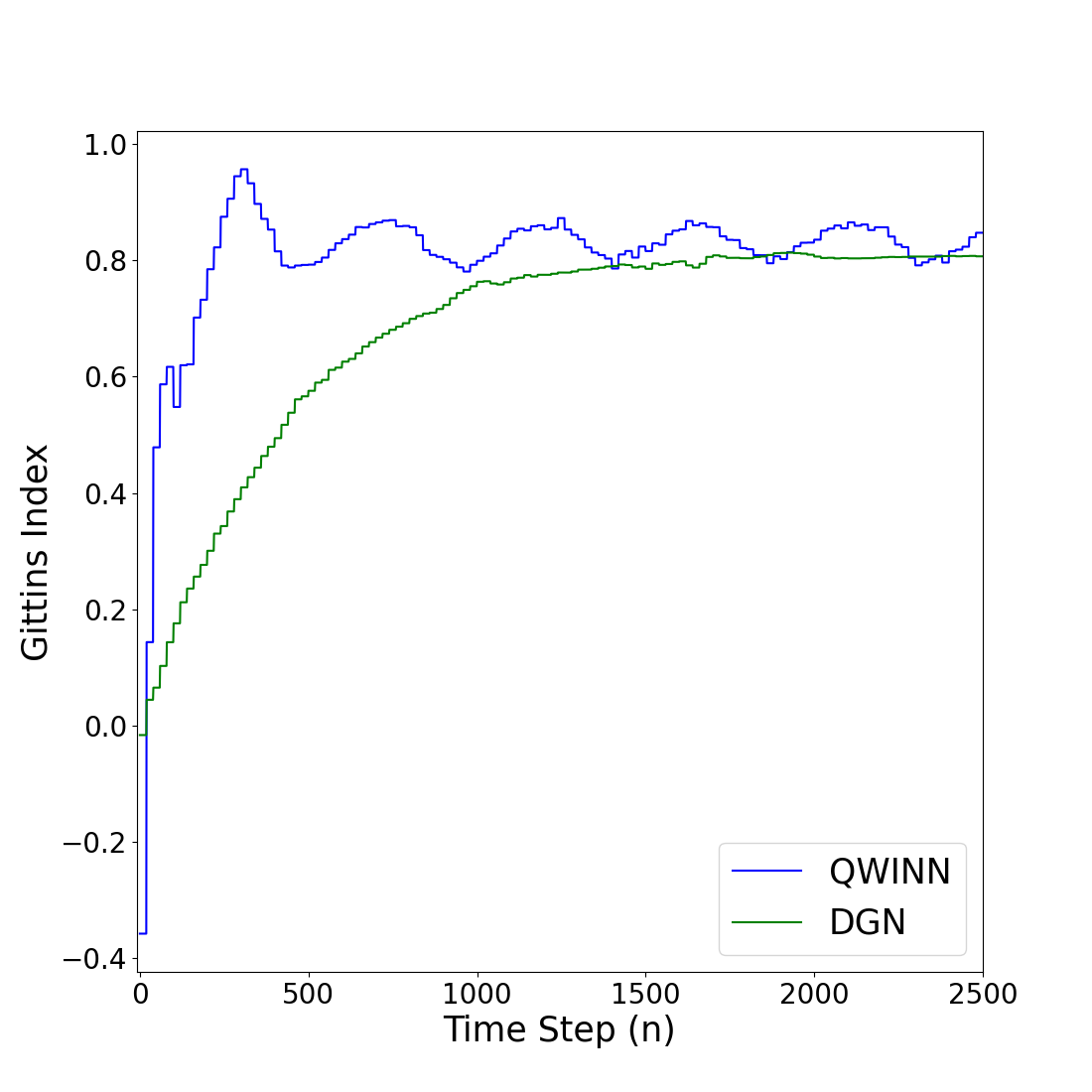
(b) State 1

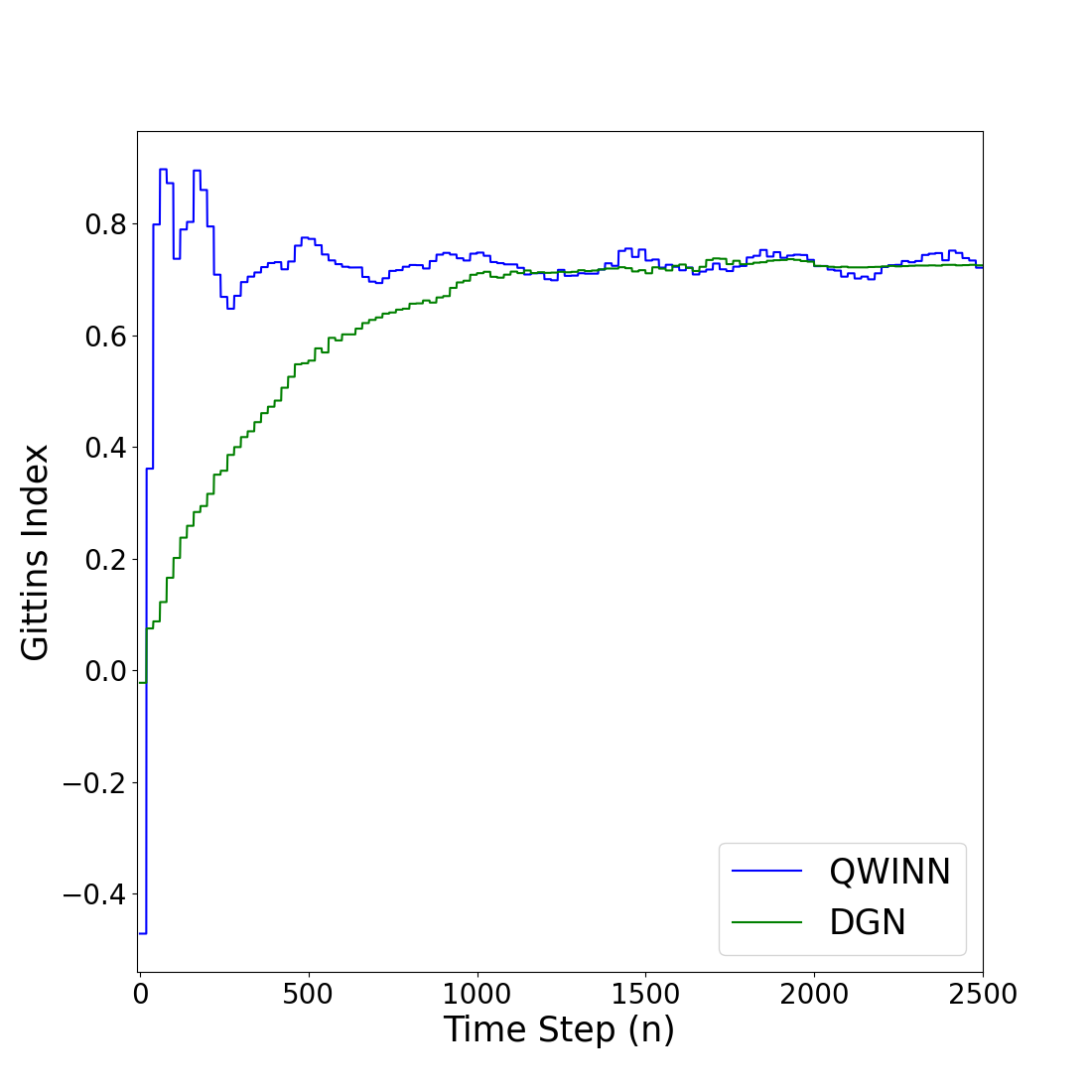
(c) State 2

Figure 2: (a), (b) and (c) show the convergence comparison of Gittins Indices for Deep-RL methods in restart problem.

V Application in Scheduling

Consider a system with a single server and a given set of $K$ jobs available at time 0. The service times of these jobs are sampled from an arbitrary distribution denoted by $F(\cdot)$. Jobs are preemptive, i.e., their service can be interrupted and resumed at a later time. For any job scheduling policy $\pi$, let $T_{i}$ denote the completion time of job i and $L^{\pi}:=\sum_{i=1}^{K}T_{i}$ denote the flowtime. A scheduling policy that minimizes the mean flowtime is the the Gittins index based scheduling policy [4, 3]. To model this problem as an MAB, note that, each job corresponds to an arm and the current state of an arm is the amount of service that the job has received till now (known as the age of the job). There is no reward from pulling an arm (serving a job) untill it has received complete service. We receive a unit reward once the required service is received. See [4, 3] for more details on the equivalence between the the flowtime minimization problem and the MAB formulation as stated above.

We are particularly interested in the setting of this problem where the job size distribution $F(\cdot)$ is not known and a batch of $K$ jobs are made available episodically. We want to investigate if the proposed algorithms QGI and DGN are able to learn the optimal Gittins index based job scheduling policy when the service time distributions $F(\cdot)$ are unknown. The problem has also been considered in [15] for learning the optimal scheduling policy with a select set of discrete job size distributions. Section V-A considers this problem where job have service time distributions with either constant or monotonic hazard rates. We also consider other discrete distributions (Poisson, Geometric and Binomial) and illustrate the empirical episodic regret from using our algorithm. Then in section V-B, we consider continuous job size distributions where each pull of an arm corresponds to giving a fixed quanta of service (denoted by $\Delta$). This allows us to discretize the problem for efficient implementation. More specifically, we consider uniform and log-normal service time distribution for our experiments. For a vanishingly small choice of $\Delta$, the state space (possible ages a job can have) becomes arbitrarily large which is when the space saving advantage of our algorithms becomes more apparent.

Note that in all the experiments below, we found QWI/QWINN to have a very poor performance in the scheduling problem. At this point, it is not clear to us why this is the case. This may be because we have not been able to figure out the right set of hyperparameters for QWI/QWINN, although we have made an extensive search for the same. Another possible reason could be the fact that passive arms are subsidised and also result in Q-value updates which may deflect the indices a lot causing poor convergence. We therefore compare our results with only that of Duff [15]. Applying QWI/QWINN for the scheduling problem is part of future work.

V-A Discrete service time distribution

We first consider the case when the job size distribution are discrete and have a possibly state dependent parameter as described below. This example is taken from [15]. Each of the $K$ jobs represent an arm which start each episode in state 1 which denotes that no service has yet been given. When an arm $i$ (read job $i$) in state $s_{n}(i)$ (with age $s_{n}(i)$) is picked/served at the $n^{th}$ step, the agent observes a transition either to $s_{n+1}(i)=s_{n}(i)+1$ of service) with probability $1-\rho^{s_{n}(i)}(i)$ or to $s_{n+1}(i)=0$ with probability $\rho^{s_{n}(i)}(i)$ if the job is completed. Upon completing a job the agent receives a reward of 1, zero otherwise. We assume that jobs that have completed service leave the system and are not available.

V-A1 Constant Hazard Rate

: We first consider the case when jobs have a Geometric distribution with parameter $\rho(i)$ for the $i^{th}$ job. Clearly, jobs are heterogeneous in nature and their transition probabilities are state independent and satisfy $\rho^{s(i)}(i)=\rho(i)$. In our experiments, we chose $10$ jobs with corresponding $\rho(i)$’s sampled uniformly from the unit interval $[0,1]$ before starting the experiment. We set $\gamma=0.99$, $\epsilon=0.1$, $\alpha(n)=0.4$ and $\beta(n)=0.2\times 1_{\{n~{}modulo~{}10\equiv 0\}}$ respectively. Here the optimal scheduling policy is known to choose jobs in the order of decreasing hazard rates. We compare the convergence behavior of our algorithm with that of [15] for a particular state $1$ and a particular arm (job 6) in Fig. 3(a). We observe that DGN converges more smoothly than tabular methods while QGI indices initially increase more quickly before settling to the optimal value.

V-A2 Monotonic Hazard Rates

Now, we consider the case of monotonically increasing and decreasing hazard rates. As in Duff [15], we consider jobs where the hazard rate changes monotonically as the job receives service. Furthermore, these hazard rate parameters are updated in an exponential fashion using a parameter $\lambda$. In our experiment we assume there are $9$ jobs, i.e., $K=9$ and the maximum state is 49, i.e, $N=50$. Before starting the trials, we sample the initial hazard rates ($\rho^{(1)}(i)$ for all $i$) uniformly from $[0,1]$. Let $\tau_{i}$ denote the random service time for the $i^{th}$ job. We assume that the disribution for $\tau_{i}$ satisfies the following :
a) For increasing hazard rate:

$$\operatorname{Pr}\left\{\tau_{i}=s\right\}=\rho^{s}(i)\prod_{k=1}^{s-1}\left(1-\rho^{(1)}(i)\right)\lambda^{k-1}\text{~{}where~{}}$$

$$\rho^{s}(i)=\left\{1-\left[\left(1-\rho^{(1)}(i)\right)\lambda^{(s(i)-1)}\right]\right\}$$

b) For decreasing hazard rate:

$$\operatorname{Pr}\left\{\tau_{i}=s\right\}=\rho^{s}(i)\prod_{k=1}^{(s-1)}\left(1-\rho^{(1)}(i)\right)\lambda^{1/(k-1)}\text{~{}where~{}}$$

$$\rho^{s}(i)=\left\{1-\left[\left(1-\rho^{(1)}(i)\right)\lambda^{1/(s(i)-1)}\right]\right\}$$

We set $\lambda=0.8$, $\gamma=0.9$ and $\epsilon=0.1$. Again, we ran our proposed algorithms for the case where all jobs have either an increasing or decreasing hazard rate. Note that the scheduling policies learnt by our algorithm coincide with the known optimal policies of FIFO and Round-Robin for increasing and decreasing hazard rates respectively. For a performance comparison among the tabular and Deep-RL methods, we consider the convergence of state 4 of job 2. Results are presented in Fig. 3(b) and  3(c).

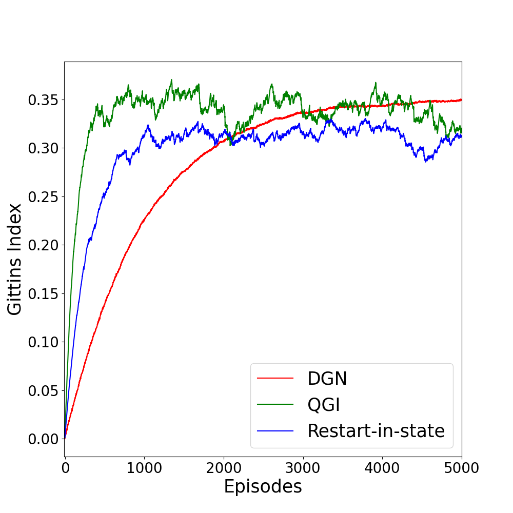
(a)

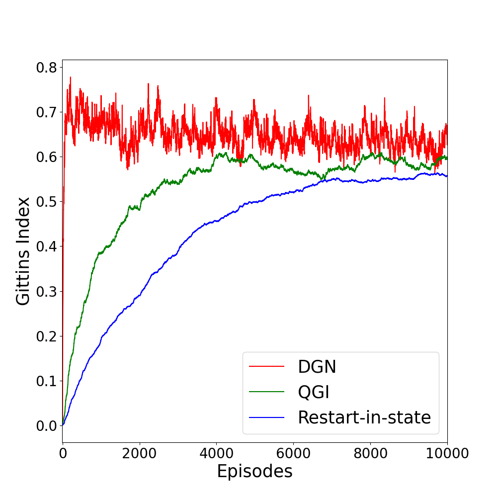
(b)

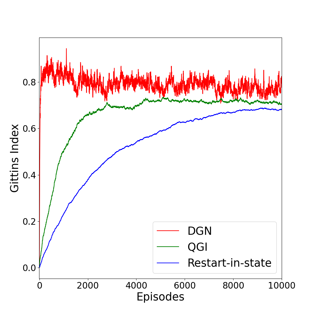
(c)

Figure 3: Performance comparison of the QGI, DGN and Restart-in-state for: (a) Constant hazard rates, (b) Increasing hazard rates and (c) Decreasing hazard rates.

V-A3 Other distributions

In this section we consider some more discrete job size distributions, specifically the Binomial$(n,p)$, Poisson($\Lambda$) and Geometric$(q)$ distributions. We consider a batch of 4 jobs in every episode. When an arm $i$ (read job $i$) in state $s_{n}(i)$ (with age $s_{n}(i)$) is picked/served at the $n^{th}$ step, the server observes a transition to $s_{n+1}(i)=s_{n}(i)+1$ as long as $\tau_{i}\neq s_{n}(i)+1$. If $\tau_{i}=s_{n}(i)+1$, then the job has received complete service and is removed from the system after earning a unit reward. In our experiment with the three distributions we choose the parameters $n=10,p=0.5,\lambda=5$ and $q=0.5$. We take $\alpha(n)=0.3$, $\beta(n)=0.2$, $\gamma=0.99$ and epsilon is set to 1 initially an decays as $\epsilon_{n+1}=max(\epsilon_{n}\times 0.9999,0.1)$. In Fig.4(a), 4(b) and 4(c) we compare the performance of QGI with restart-in-state (for states $1,2,~{}and~{}3$) for Binomial, Poisson and Geometric distribution respectively. While the speed of convergence depends on the type of distribution considered and the corresponding states, QGI seems to outperform restart-in-state for all states and all distributions considered.

In Fig. 5(a), we plot the percentage of time QGI and restart-in-state chose the optimal action as a function of the iteration number for the three distributions. Here again QGI displays a better accuracy, especially for the Poisson and Binomial distribution. We also plot the cumulative episodic regret for the two algorithms (for all the three distributions). Here the episodic regret was calculated as the difference in the flowtime between QGI and the optimal Gittins index policy in an episode. Again, we see that the cumulative regret for QGI is lower than restart-in-state-i, clearly demonstrating the advantages of our method.

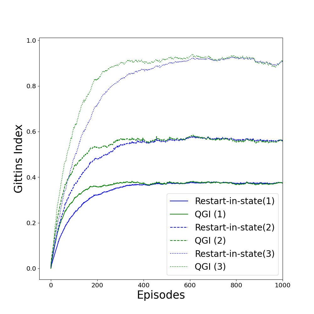
(a)

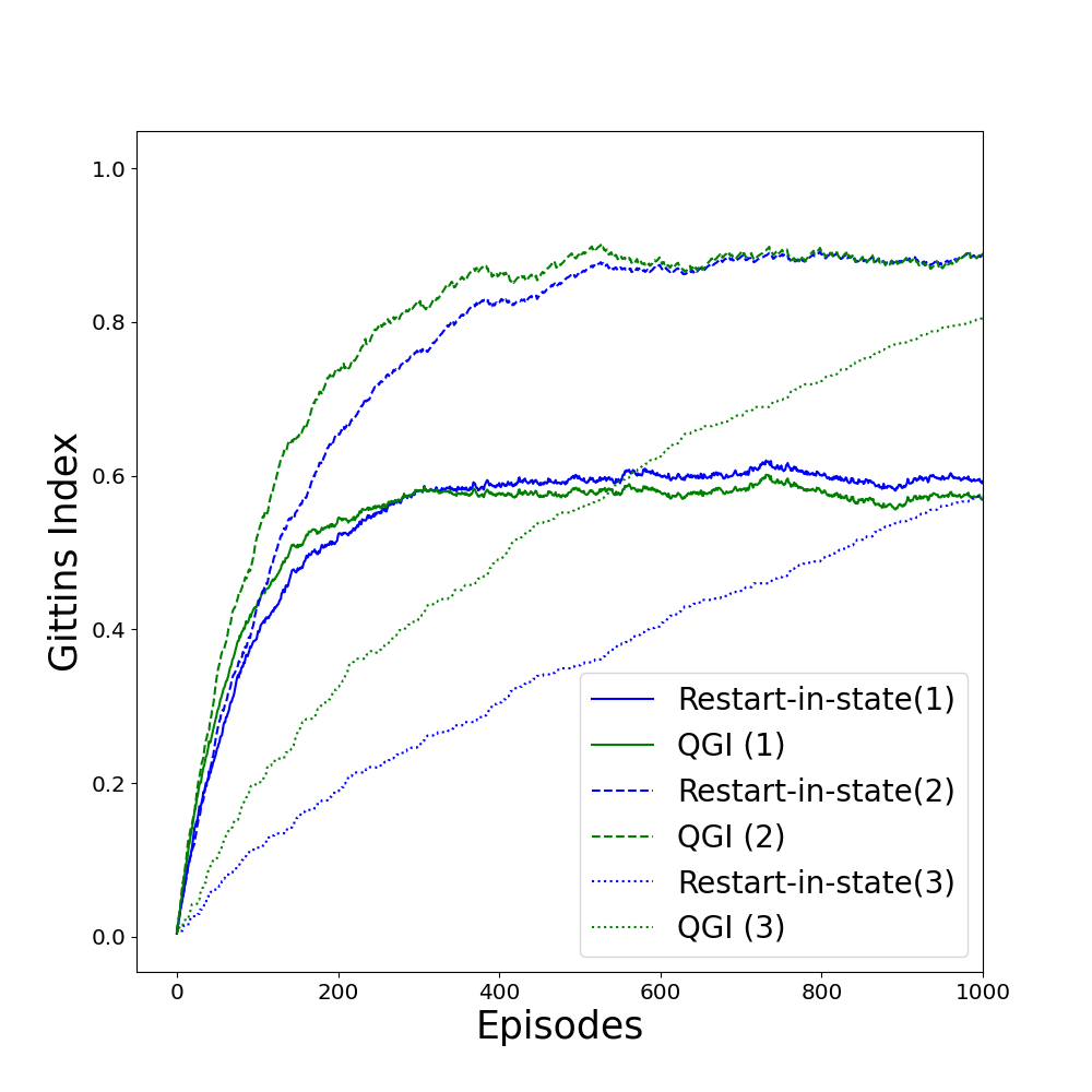
(b)

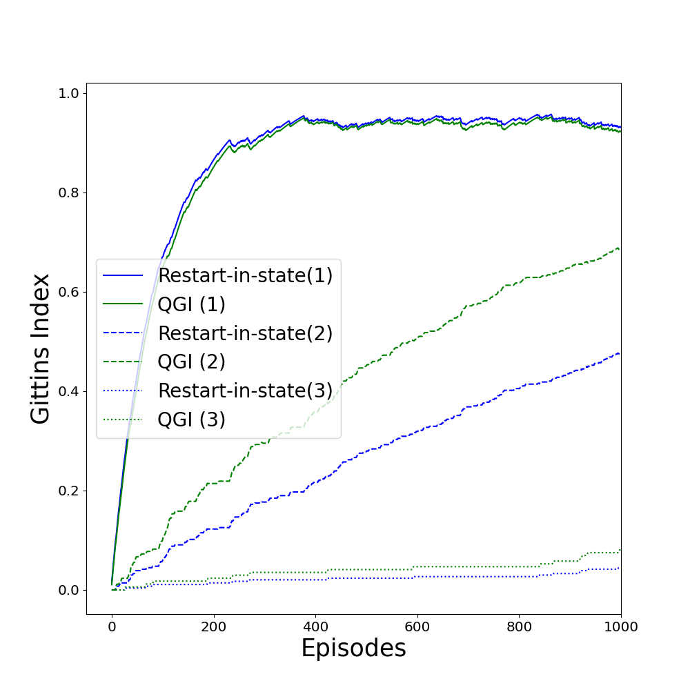
(c)

Figure 4: Convergence of Gittins Indices for (a) Binomial, (b) Poisson and (c) Geometric service time distributions.

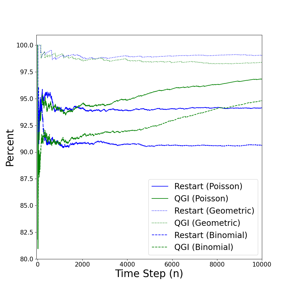
(a)

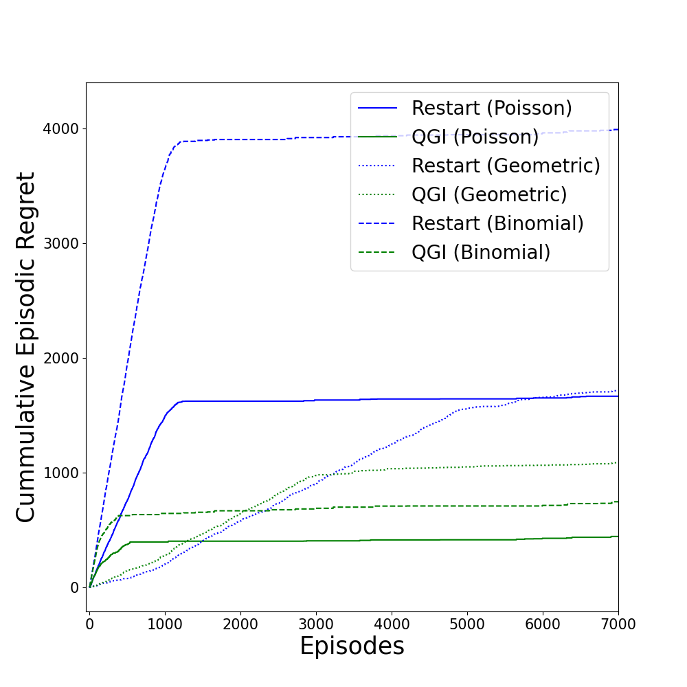
(b)

Figure 5: (a) shows the $\%$ of steps for which an optimal action is performed while (b) shows the cumulative episodic regret collected over trials.

V-B Continuous service time distribution

We now consider some continuous service time distribution for job sizes. For our experiment we consider a batch of $4$ jobs per episode. Service is provided in a fixed quanta of size $\Delta$ that allows us to discretize the problem and use the existing machinery. Once a $\Delta$ is fixed, we have a discrete time MAB where the age of jobs are discrete multiples of $\Delta$. As in section V-A3, when an arm $i$ in state $s_{n}(i)$ is picked/served at the $n^{th}$ step, the server observes a transition to $s_{n+1}(i)=s_{n}(i)+1$ as long as $\tau_{i}\neq s_{n}(i)+1$.

We first consider the experiment where job sizes are Uniform over the support $[0,10]$ and a service quantum of size $\Delta=0.1$. This makes the number of possible states in the system equal to 100. There are $4$ jobs in each episode to schedule and the discount factor $\gamma=0.9$ is considered. The performance results are shown in Fig. 6(a) for state 34 (age 3.4). It can be seen that both the tabular methods have more variability as compared to DGN which converges more smoothly. We next assume that the job sizes are sampled from a log-normal distribution with parameter $\mu=log(30),\sigma=0.6$ and $\Delta=0.5$. We truncate the max job size to 75 (as $P(X>75)$ = $0.06336$). Here, again four homogeneous jobs are taken per episode and the discount factor is $\gamma=0.9$. Note that the number of states, $|S|=150$. Due to this, the number of Q-values being tracked in QGI are 100,100 while in other algorithms 2,00,000 cells are being filled. The performance results for a particular state 49 (age 24.5) are shown in Fig. 6(b).

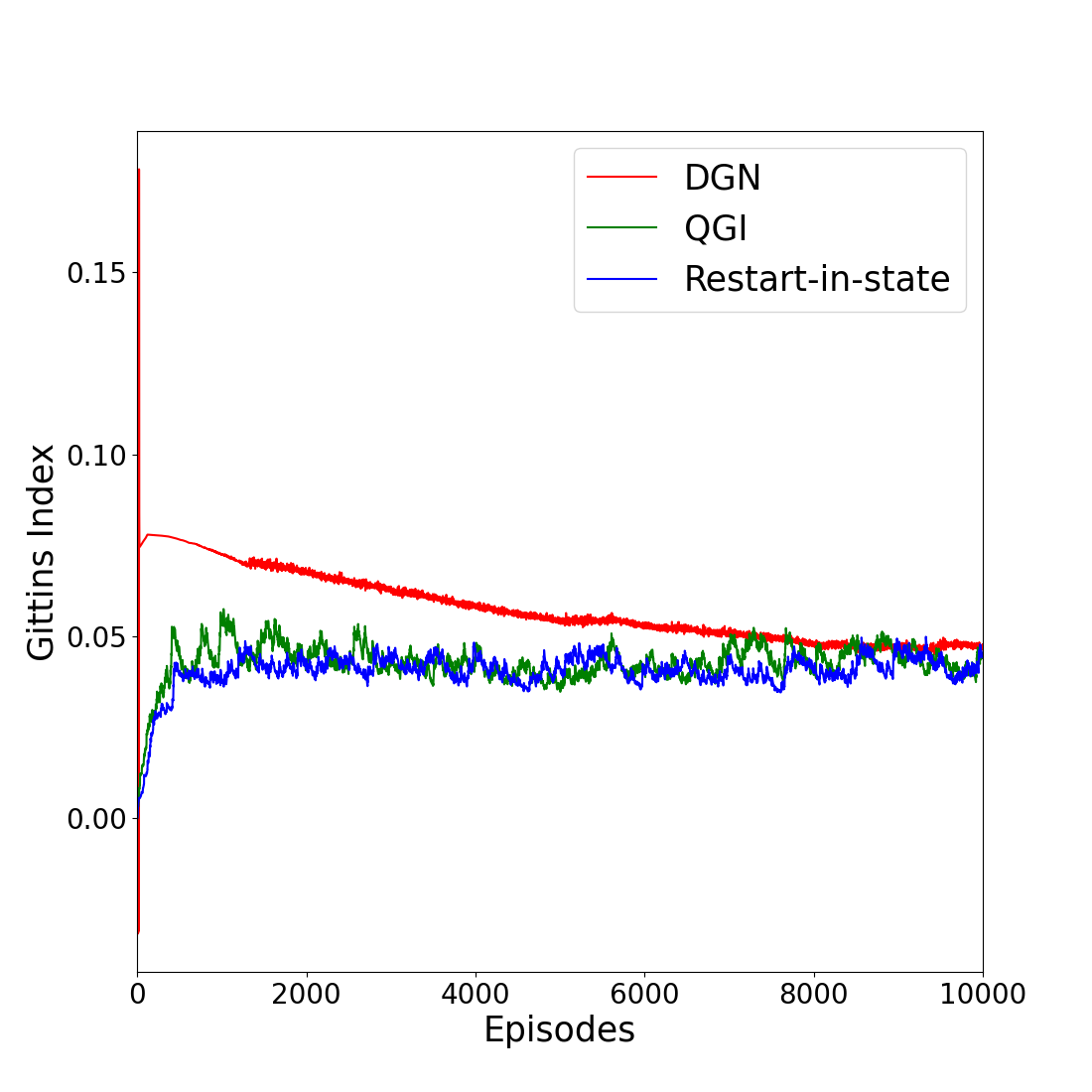
(a)

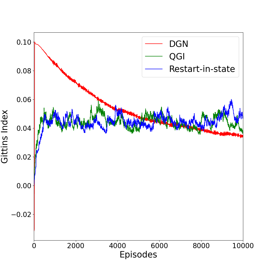
(b)

Figure 6: Performance comparison of the QGI, DGN and Restart-in-state for: (a) Uniform distribution and (b) Log normal distribution.

VI Conclusion

In this work, we have introduced QGI and DGN which are tabular and deep RL based methods for learning the Gittins indices using the retirement formulation. To illustrate the applicability of our method, we consider the problem of learning the optimal scheduling policy that minimizes the mean flowtime for batch of jobs with arbitrary but unknown service time distributions. Through our experiments, we have shown that our methods have better convergence performance, require less memory and also offer lower empirical cumulative regret. There are several open directions that beg further investigation. First, we would like to identify the reason for a poor performance of QWI/QWINN on the scheduling problem. We would also like to investigate the applicability of our method to learning the optimal scheduling policy in an $M/G/1$ queue minimizing the mean sojourn time. While the algorithms that we propose and those that are in the literature are essentially value function based, we would also like to see if a policy gradient based approach can be used to learn the Gittins index.

Appendix 1. Proof outline for Theorem 1: The proof follow along similar lines to that in [18]. Also see [24] for similar results. Consider the following equations which will be compared to equations (8) and (13) later:

$$x_{n+1}=x_{n}+a(n)\left[h\left(x_{n},y_{n}\right)+L_{n+1}^{(1)}\right]$$ (16)

$$y_{n+1}=y_{n}+b(n)\left[g\left(x_{n},y_{n}\right)+L_{n+1}^{(2)}\right]$$ (17)

In these equations, the functions $h$ and $g$ are continuous Lipschitz functions, the $L_{n}$ are martingale difference sequences representing noise terms, and $a(n)$ and $b(n)$ are step-size terms satisfying $\sum_{n}\alpha(n)=\infty,\sum_{n}\alpha(n)^{2}<\infty$, $\sum_{n}\beta(n)=\infty,\sum_{n}\beta(n)^{2}<\infty$ and $\frac{b(n)}{a(n)}\rightarrow 0$ as $n\rightarrow\infty$. These conditions are necessary for stable convergence of (16) and (17). Note that, for notational convenience, we use $M_{x}(n)$ to denote the value of Gittins estimate of state x in $n^{th}$ iteration. Here, (16) represents the Q-learning update as in (8) and (17) represents equation the stochastic approximation step to update the indices as in (13). First, let us define $F_{s}^{M}(\Psi(j,b))$ and $L_{n+1}(s)$ such that:

$$F_{s}^{M}(\Psi(j,b))=R(s)+\gamma\sum_{j}p(j\mid i,u)\max\left\{\Psi(j,1),M_{j}\right\}$$

$$L_{n+1}(s)=R(s)+\max\left\{Q_{n}^{x}\left(s_{n+1},1\right),M_{n}(x)\right\}-F_{s}^{M_{x}(n)}\left(Q_{n}\right).$$

Using these, we can rewrite the equation (8) as:

$$Q_{n+1}^{x}(s,u)=Q_{n}^{x}(s,u)+\alpha(n)\left[F_{s}^{M_{x}(n)}\left(Q_{n}\right)-Q_{n}^{x}(s,u)+L_{n+1}(s)\right]$$ (18)

Comparing equations (16) and (18) we can make the correspondence $a(n)=\alpha(n),h\left(x_{n},y_{n}\right)=F_{s}^{M_{x}}(n)\left(Q_{n}\right)-Q_{n}$, where $x_{n}=Q_{n}$, $y_{n}=M(n)$ and $L_{n+1}(s)$ is the martingale difference sequence $L_{n+1}^{(1)}$. Equations (13) and (17) correspond to $b(n)=\beta(n)$, $g\left(x_{n},y_{n}\right)=Q_{n}^{x}(x,1)-M_{x}(n)$ and a martingale difference sequence $L_{n+1}^{(2)}=0$.

Now let $\tau(n)=\sum_{m=0}^{n}\alpha(m),m\geq 0$. Define $\bar{Q}(t),\bar{\lambda}(t)$ as the interpolation of the trajectories of $Q_{n}^{x}$ and $M_{x}(n)$ on each interval $[\tau(n),\tau(n+1)],n\geq 0$ as:

$$\begin{gathered}\bar{Q}(t)=Q(n)+\left(\frac{t-\tau(n)}{\tau(n+1)-\tau(n)}\right)(Q(n+1)-Q(n))\\ \bar{M}_{x}(t)=M_{x}(n)+\left(\frac{t-\tau(n)}{\tau(n+1)-\tau(n)}\right)(M_{x}(n+1)-M_{x}(n))\\ t\in[\tau(n),\tau(n+1)]\end{gathered}$$

which track the asymptotic behavior of the coupled o.d.e.s

$$\dot{Q}(t)=h(Q(t),M_{x}(t)),\dot{M_{x}}=0$$

Here the latter is a consequence of considering the following form of equation (13) and putting $\frac{\beta(n)}{\alpha(n)}\rightarrow 0$:

$$M_{x}(n+1)=M_{x}(n)+\alpha(n)\left(\frac{\beta(n)}{\alpha(n)}\right)\left(Q_{n}^{x}(x,1)-M_{x}(n)\right)$$

Now, $M_{x}(\cdot)$ is a constant of value $M_{x}^{\prime}$ for $Q(t)$ due to $M_{x}(\cdot)$ being updated on a slower time scale. Because of this, the first o.d.e. becomes $\dot{Q}=h\left(Q(t),M_{x}^{\prime}\right)$, which is well posed and bounded, and has an asymptotically stable equilibrium at $Q_{M}^{*}$ [Theorem 3.4, [25]]. This implies that $Q_{n}^{x}-Q_{M_{x}(n)}^{*}\rightarrow 0$ as $n\rightarrow\infty$. On the other hand, for $M_{x}(t)$, let us consider a second trajectory on the second time scale, such that:

$$\begin{array}[]{r}\tilde{M}_{x}(t)=M_{x}(n)+\left(\frac{t-\tau^{\prime}(n)}{\tau^{\prime}(n+1)-\tau^{\prime}(n)}\right)(g(n+1)-g(n))\\ t\in\left[\tau^{\prime}(n),\tau^{\prime}(n+1)\right],\tau^{\prime}(n)=\sum_{m=0}^{n}\beta(m),n\geq 0\end{array}$$

which tracks the o.d.e.:

$$\dot{M}_{x}(t)=Q_{M_{x}(t)}^{*}(x,1)-M_{x}(t)$$

As in the previous case this bounded o.d.e converges to an asymptotically stable equilibrium where $M$ satisfies $Q_{M}^{*}(x,1)=M_{x}$. This is the point of indifference between retiring and continuing, and hence, $M$ characterises the Gittins index.

References

- [1] J. Gittins, “A dynamic allocation index for the sequential design of experiments,” Progress in statistics, pp. 241–266, 1974.
- [2] T. Lattimore and C. Szepesvári, Bandit algorithms. Cambridge University Press, 2020.
- [3] M. L. Pinedo, Scheduling. Springer, 2012, vol. 29.
- [4] J. Gittins, K. Glazebrook, and R. Weber, Multi-armed bandit allocation indices. John Wiley & Sons, 2011.
- [5] Z. Scully, “A new toolbox for scheduling theory,” ACM SIGMETRICS Performance Evaluation Review, vol. 50, no. 3, pp. 3–6, 2023.
- [6] S. Aalto, U. Ayesta, and R. Righter, “On the gittins index in the M/G/1 queue,” Queueing Systems, vol. 63, pp. 437–458, 2009.
- [7] Z. Scully, I. Grosof, and M. Harchol-Balter, “The gittins policy is nearly optimal in the M/G/k under extremely general conditions,” Proceedings of the ACM on Measurement and Analysis of Computing Systems, vol. 4, no. 3, pp. 1–29, 2020.
- [8] S. Aalto and Z. Scully, “Minimizing the mean slowdown in the M/G/1 queue,” Queueing Systems, vol. 104, no. 3, pp. 187–210, 2023.
- [9] J. C. Gittins, “Bandit processes and dynamic allocation indices,” Journal of the Royal Statistical Society Series B: Statistical Methodology, vol. 41, no. 2, pp. 148–164, 1979.
- [10] J. N. Tsitsiklis, “A short proof of the gittins index theorem,” The Annals of Applied Probability, pp. 194–199, 1994.
- [11] E. Frostig and G. Weiss, “Four proofs of Gittins’ multiarmed bandit theorem,” Annals of Operations Research, vol. 241, no. 1-2, pp. 127–165, 2016.
- [12] P. Whittle, “Restless bandits: Activity allocation in a changing world,” Journal of applied probability, vol. 25, no. A, pp. 287–298, 1988.
- [13] R. R. Weber and G. Weiss, “On an index policy for restless bandits,” Journal of applied probability, vol. 27, no. 3, pp. 637–648, 1990.
- [14] N. Gast, B. Gaujal, and C. Yan, “Exponential asymptotic optimality of Whittle index policy,” Queueing Systems, pp. 1–44, 2023.
- [15] M. O. Duff, “Q-learning for bandit problems,” in Machine Learning Proceedings 1995. Elsevier, 1995, pp. 209–217.
- [16] K. E. Avrachenkov and V. S. Borkar, “Whittle index based Q-learning for restless bandits with average reward,” Automatica, vol. 139, p. 110186, 2022.
- [17] F. Robledo, V. Borkar, U. Ayesta, and K. Avrachenkov, “Qwi: Q-learning with whittle index,” ACM SIGMETRICS Performance Evaluation Review, vol. 49, no. 2, pp. 47–50, 2022.
- [18] F. Robledo, V. S. Borkar, U. Ayesta, and K. Avrachenkov, “Tabular and deep learning of Whittle index,” in EWRL 2022-15th European Workshop of Reinforcement Learning, 2022.
- [19] K. Nakhleh, I. Hou et al., “Deeptop: Deep threshold-optimal policy for MDPs and RMABs,” Advances in Neural Information Processing Systems, vol. 35, pp. 28 734–28 746, 2022.
- [20] H. Van Hasselt, A. Guez, and D. Silver, “Deep reinforcement learning with double Q-learning,” in Proceedings of the AAAI conference on artificial intelligence, vol. 30, no. 1, 2016.
- [21] P. Whittle, “Multi-armed bandits and the Gittins index,” Journal of the Royal Statistical Society: Series B (Methodological), vol. 42, no. 2, pp. 143–149, 1980.
- [22] J. Chakravorty and A. Mahajan, “Multi-armed bandits, gittins index, and its calculation,” Methods and applications of statistics in clinical trials: Planning, analysis, and inferential methods, vol. 2, pp. 416–435, 2014.
- [23] T. P. Lillicrap, J. J. Hunt, A. Pritzel, N. Heess, T. Erez, Y. Tassa, D. Silver, and D. Wierstra, “Continuous control with deep reinforcement learning,” arXiv preprint arXiv:1509.02971, 2016.
- [24] V. S. Borkar, Stochastic approximation: a dynamical systems viewpoint. Springer, 2009, vol. 48.
- [25] J. Abounadi, D. Bertsekas, and V. S. Borkar, “Learning algorithms for markov decision processes with average cost,” SIAM Journal on Control and Optimization, vol. 40, no. 3, pp. 681–698, 2001.