Thermalization slowing down of weakly nonintegrable quantum spin dynamics
Abstract
We study thermalization slowing down of a quantum many-body system upon approach to two distinct integrability limits. Motivated by previous studies of classical systems, we identify two thermalization time scales: one quantum Lyapunov time scale is extracted by quantifying operator growth in time in an appropriately defined basis, while another ergodization time scale is related to statistics of fluctuations of the time-evolved operator around its mean value based on the eigenstate thermalization hypothesis. Using a paradigmatic Quantum Ising chain we find that both timescales diverge upon approach to integrability. The relative strength of the divergence of the scales depends on the particular integrable limit. This allows us to define two different universality classes of quantum thermalization: short- and long-range networks.
Introduction— The study of integrable and chaotic dynamics in quantum systems is an area of active investigation with the goal of explaining the emergence of statistical mechanics in interacting quantum systems, among others. Multiple observables have been identified and studied as probes of integrable/chaotic dynamics. One class of such probes is based on spectral properties of the system [1, 2, 3, 4, 5, 6, 7, 8] rooted in the BGS and Berry-Tabor conjectures [1, 2] and the expected random matrix-like behavior of quantum systems [9, 10]. Another class of observables is based on the operator growth or state evolution under integrable/chaotic Hamiltonians. Observables such as Out-of-time-ordered-correlation functions (OTOCs) [11, 12, 13, 14, 15, 16, 17, 18, 19, 20, 21, 22, 23], circuit complexity [24, 25, 26, 27], operator size [28, 29, 30, 31] and Krylov complexity [32, 33, 34, 35, 36, 37, 38, 39] fall into this category.
Thermalization is a closely related phenomenon to the study of chaos. It describes late-time physics at equilibrium and leads to the emergence of statistical mechanics. Thermalization is a universal property of non-integrable systems, found in both classical and quantum dynamics. Specifically, we are interested in the nature of thermalization near integrability, where it is expected to slow down. This has been explored extensively in classical systems. One of the key features studied in this respect are the relevant timescales: Lyapunov time, ergodization time, etc. These timescales are obtained by computing different observables and studying their divergence upon approach to integrability [40, 41, 42, 43, 44, 45, 46, 47, 48, 49].
In quantum mechanical systems, the Eigenstate Thermalisation Hypothesis (ETH) [50, 51, 52, 53, 54, 55, 56] is often used to characterize thermalization. Within the purview of ETH, there are ergodization time-scales (e.g. the Thouless time) [52, 57, 58] which have been explored in various systems. These time scales differ between chaotic and integrable systems, and their exact nature is studied extensively. Another active direction of investigation involves the notion of Lyapunov-like time scales for quantum systems. Operator growth serves as a potential path (via OTOCs) to define an appropriate spectrum [59, 60, 61]. Similarly, the spectral function is also used [62]. In quantum systems without well-defined classical limits (for example, spin- chains) the quantum Lyapunov spectra behave quite differently from classical spectra and may suffer from definition ambiguities [61, 60]. There are better-defined notions of the maximum Lyapunov exponent, which is typically extracted from the growth exponent of an appropriately defined observable. These include the exponent of the OTOC [63] and Krylov complexity [32, 37].
In this manuscript, we take the concept of time scales, originally developed for classical networks, to quantum mechanical systems near integrability. We introduce the notion of quantum networks near integrability and characterize them by studying the dynamics of conserved quantities of the limiting integrable Hamiltonian. We employ the operator growth approach (using Krylov complexity) to define an appropriate notion of Lyapunov time. Operator growth is captured through the lens of Krylov complexity, which describes the evolution of an operator on a minimal basis. We then use ETH principles to extract another time scale, which we coin the ergodization timescale (in analogy to classical systems). The system that we study is a prototypical 1D quantun Ising spin- chain. Near the integrable limits, these time scales are compared and used to identify two classes of quantum networks, which we call short- and long-range networks.
The model— The prototypical spin system we employ in order to characterize long and short-range networks is the Quantum Ising chain [64, 65] given by the following Hamiltonian
| (1) |
where and are real numbers describing nearest-neighbour interaction, longitudinal and transverse magnetic field respectively. The are Pauli matrices, describing spin- algebra. The system is in general non-integrable and has been extensively studied through various probes of quantum chaos [66, 67, 68, 69, 70, 71]. In the limits (TFIM) or (classical), the Hamiltonian (1) becomes integrable. We study the chaos and thermalization in the vicinity of these limits in order to observe and quantify the possible differences between the two limits.
In classical systems near integrable limits, the short and long-range networks are defined with respect to the connectivity of the actions of the integrable system. The system is defined as a long-range network if the connectivity (defined through an appropriately defined coupling range) is extensive in the number of actions . In a short-range network the connectivity of the actions (i.e. the coupling range) is independent of the number of actions.
Inspired by the classical definition, we study the conserved quantities of the TFIM in the integrable limit. In the limit , the spin chain becomes classical and the conserved quantities are local, with the simplest one being . The support of does not scale with system size and neither is it connected with the other simple conserved quantities (i.e with ). In the limit , the spin chain is extensively connected while still being integrable. This is reflected by the fact that the conserved quantities are non-local111Corresponding to the fermionic operators in the Jordan-Wigner representation of the system. Some of these operators correspond to simple symmetry operations. For example, the spin-flip operation for all spins leaves the Hamiltonian invariant. The corresponding conserved quantity is . Other conserved quantities are similarly represented as extensive (non-local) combinations of the local spin matrices. The support of such quantities grows with system size.
Thus, we define (by analogy to the classical definition [46, 47, 45]), the following two types of networks: (i) Quantum short-range network (SRN)—A system that is weakly nonintegrable, where the conserved quantities corresponding to the integrable part are connected by the nonintegrable perturbation in a short-ranged way, as observed from the operator dynamics defined by standard commutator relations. (ii) Quantum long-range network (LRN)—A system that is weakly nonintegrable, where the conserved quantities corresponding to the integrable part are connected in a non-local all-to-all way by the nonintegrable perturbation and their operator dynamics.
In what follows, we probe the timescales and ergodicity properties of operators near the two respective limits and study time scales related to the ETH-like behavior of the observables. We then compare the divergence of these two time-scales – ETH-related and related to the operator growth – in the vicinity of the two limits.
Krylov complexity— There exists a large class of observables that quantify operator growth under Hamiltonian dynamics. A common feature among most of these probes is the choice of a basis to expand the time-evolved operator. Once the basis is chosen, then appropriate expectation values are defined and evaluated, which then serve to distinguish between chaotic and integrable systems.
One such probe is Krylov complexity [32]. The steps to evaluate Krylov complexity begin with generating a minimal basis 222Minimal with respect to a cost function; which in this case is the Krylov complexity itself., which is called the Krylov basis. The Krylov complexity captures the average position of an operator in the minimal basis under the operator’s unitary evolution in time with the Hamiltonian . The construction of the Krylov basis relies on an appropriately chosen norm in the Hilbert space of operators. We employ the infinite-temperature Hilbert-Schmidt norm for our analysis:
| (2) |
Upon adopting the norm, one chooses an operator whose evolution is studied. The unitary evolution of governed by the Hamiltonian is defined as
| (3) |
where is the Louivillian superoperator. The elements of the minimal (Krylov) basis corresponding to the operator and Hamiltonian are generated via the Lanczos algorithm [74, 32], as described in the Supplementary Material. The operator has the following expansion in this basis
| (4) |
The dynamical properties of under the Hamiltonian are encoded in the behavior of the Krylov wavefunctions . These properties allow to diagnose chaotic behavior in quantum many-body systems [32, 37, 38, 34, 35, 36].
It was argued in Ref. 32 that the average position of the time-evolved operator
| (5) |
known as Krylov complexity, grows exponentially with for chaotic dynamics: . The exponent captures the strength of the chaotic dynamics and is bounded from above by the Maldacena-Shenker-Stanford [63] bound. One can then define a natural time-scale for a chaotic system as , which we denote as throughout this manuscript, since it captures the growth of operators under the Hamiltonian .
Ergodization time— Eigenstate thermalization hypothesis [50, 54] provides a powerful tool to study and characterize thermalization in quantum mechanical systems. It serves as a way to probe the chaotic or integrable dynamics of a system through evolution of operators and states. The essential statement of ETH can be encapsulated in the following equation
| (6) |
where the expectation value of the time-evolved operator is taken in a typical state and the long time-averaged expectation value of the operator can be evaluated analytically in the diagonal ensemble. The function represents subleading fluctuations, suppressed by the Hilbert space dimension . The nature of the function has been studied extensively in different chaotic and integrable systems [75, 76, 77, 78].
We use the fluctuations of to extract a timescale, that we refer to as the ergodization timescale . The definition of this scale largely follows that in the classical case, discussed in Ref. 40. We choose a random initial state as the typical state and track the evolution of . As the function evolves it eventually starts to fluctuate around the mean value , going above and below the mean with time. This defines the passage times of the function across the mean value: [46, 47, 45, 44, 43, 42, 41, 40]. Time intervals between the two subsequent passages
| (7) |
are called excursion times, since they reflect the time spent by the expectation value away from its mean value. We distinguish additionally positive, , and negative, excursions times for excursions above and below the mean value . For a given system and operator, the collected excursion times obey some distribution. We use use the moments—mean and variance—of this distribution to extract an ergodization time-scale, as defined later and discussed in the Supplementary Material.
Results— We study numerically the dynamical properties close to integrability of the quantum short- and long-range networks respectively using the definitions and the methods outlined above. The Hamiltonian is given by Eq. (1) and we pick the two conserved quantities in the two integrable limits of the Hamiltonian
| (8) | ||||
| (9) |
as the time-evolved operators/observables whose dynamical properties we study. Other choices of operators yielded similar results. Naturally, at the integrable limits, the operators are conserved, their corresponding Lyapunov exponents are and their Lyapunov times definhed through the Krylov complexity diverge. Similarly to the classical case, we are interested in quantifying the divergence of the Lyapunov and ergodization times (from the two probes) upon approaching the integrable limits.
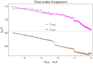
Figure 1 shows the Lyapunov times extracted from the linear growth of the Lanczos coefficients in the Krylov basis of the operators (8-9) and plotted in the log-log scale as functions of the integrability breaking parameters (LRN) or (SRN). In both cases the observed behavior of suggests a power-law divergence for small values of or . The exponents are extracted for a system of spins via a linear fit of the data on the log-log scale
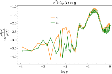
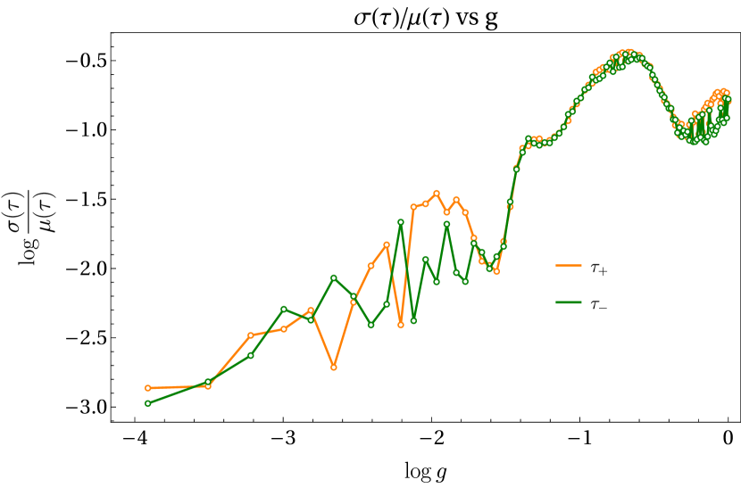
To study the thermalization properties, we collect the statistics of the excursion times (7) of the expectation value of the respective operators (8-9) in a random state (different choices of the state yielded similar results). We study the mean and variance of the positive and negative excursion times (7). To define an appropriate ergodization time , we study the relative behavior of mean and variance by collecting excursions. Increasing this number does not change the moments significantly. The following behavior of the moments is observed, that follows rather closely the classical weakly nonintegrable systems: For SRN the values of are times greater than the close to integrability. This suggests that the typical timescale of fluctuations is dominated by the distribution tail rather than its mean. A natural ergodization timescale is then defined as [46, 47, 45, 44, 43, 42, 41, 40]. For LRN the values of the variance are of the order of the mean . This suggests that the dynamics receive comparable contributions from the mean as well as fluctuations of the crossing times. The ratio of variance and mean is approximately constant near the integrable limit and does not change considerably as is varied. We define ergodization time as the mean , but the variance is a valid choice as well.
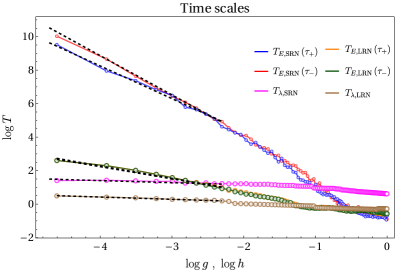
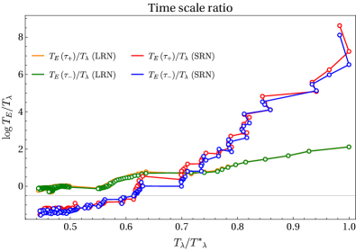
In Fig. 2 we compare the ergodization times for the SRN and LRN based on positive/negative excursion times with the Lyapunov time obtained via the Krylov method. Similarly to the Laypunov time the ergodization time also shows a power-law divergence with the decrease of the integrability breaking parameter. The linear fits of the data in the log-log scale are
where stands for the timescales extracted from the positive and negative excursion times. Ergodization times extracted from positive and negative excursion times show similar scaling close to integrability.
A central observation is the different relative scaling of and upon approach to integrability for SRN and LRN, which serves as a marker for short- and long-range networks, and is similar to that of the classical long- and short-range networks. In Fig. 2 becomes larger than by several orders of magnitude for the short-range network (SRN) as integrability is approached. This is due to the fact that the decay exponent for is times the decay exponent for in this case. Consequently as integrability is approached, the ergodization times diverges much faster than the Lyapunov times. A similar observation was also made for the classical SRN [45].
For the long-range network (LRN), remains comparable to close to integrability. The decay exponent of is of the same order as the decay exponent for . The ergodization and Lyapunov times therefore diverge in a similar fashion upon approaching integrability.
This suggests a universality of thermalization slowing down in quantum many-body systems based on the emergence of two distinct network classes. The short-range networks, characterized by local conserved quantities in the integrable limit, show a much faster slowing down of thermalization as compared to operator growth. Long-range networks, characterized by non-local conserved quantities in the integrable limit, show a comparable slowing down of thermalization and operator growth.
This is further emphasized in Fig. 3, which shows the ratio as a function of . Here is the maximum value of for each (SRN, LRN) of the networks and is required for an effective comparison of the two networks, since the range of observed in Fig. 1 is different for the SRN and LRN networks. It is evident from Fig. 3 that for the short-range network, scales as with , especially near . For the long-range network, scales approximately as .
Conclusions— In this manuscript, we extended the universality classes of thermalization of classical weakly non-integrable systems to the case of weakly non-integrable quantum many-body systems. The classes are defined by the two timescales quantifying thermalization: one timescale comes from the Krylov complexity of operator growth. In the non-integrable regime, the K-complexity grows as , defining a Lyapunov timescale. Another timescale, the ergodization time , is inspired by ETH and is defined through the statistics of the time intervals between consecutive crossings of the expectation of time-evolved operator around its mean value . is then defined through the appropriate moments of the intervals. For conserved in the intergable limit, both timescales are expected to diverge.
The short-range network (SRN) is defined by the locality of interaction between the conserved quantities (in the integrable limit) as integrability is weakly broken. We find that the distribution of the crossing intervals is fat-tailed in this case and therefore is defined as the ratio of the variance and the mean. Conversely, the long-range network (LRN) is defined by the non-locality of interaction between the conserved quantities upon weak integrability-breaking. Then the first two moments of the distribution of the crossing intervals are comparable and thus we define as the mean of the distribution.
In the 1D spin- chain we study, both timescales, and , diverge as power-laws with decreasing integrability breaking parameter. We compare the exponents of both and in the two network classes. We find that the exponents of and are comparable to each other for LRN. This indicates that the rate at which thermalization (in the ETH sense) slows down upon approaching the integrable limit is comparable to the slowing down of operator spreading. We identify this as a distinguishing feature of the long-range quantum networks. The exponent for is found to be larger than by at least an order of magnitude for SRN. This is indicative of the fact that ETH-like thermalization slows down exponentially faster than operator spreading as integrability is approached.
We identify this drastic difference in the relative slow-down of thermalization and operator spreading as the distinguishing feature of short- and long-range networks. This is consistent with the character of thermalization slowing down in classical systems [41, 40] where classical Lyapunov time is compared to the classical ergodization time, and generalizes the notion of classical networks to quantum many-body systems.
Many open questions naturally emerge from this investigation. One natural direction is testing this classification for other systems. Further, other probes might be able to distinguish and be sensitive to these two network classes. In the classical case the Lyapunov spectrum scaling close to integrability proved to be instrumental in classifying network classes [41]. It would interesting to study probes that do not have classical analogues, such as quantum entanglement [79]. Our investigation was restricted to finite system sizes, the scaling of the two timescales with system size (and therefore in the thermodynamic limit) is worth investigating. There has also been a large body of work that has investigated the exact nature of the fluctuations of operator evolution (for example, in Eq. (6)). This suggests that a more concrete connection between ETH and ergodization time might exist. Random matrix theory is also expected to play a crucial role in this characterization. It would also be interesting to study the effective random matrix theory near integrability for the two network classes.
Acknowledgments— The authors acknowledge Tilen Cadez, Barbara Dietz, Yeongjun Kim, Gabriel Lando, Aniket Patra, Sonu Verma and Weihua Zhang for relevant discussions. We acknowledge the financial support from the Institute for Basic Science (IBS) in the Republic of Korea through the Project No. IBS-R024-D1.
References
- Bohigas et al. [1984] O. Bohigas, M. J. Giannoni, and C. Schmit, Characterization of chaotic quantum spectra and universality of level fluctuation laws, Phys. Rev. Lett. 52, 1 (1984).
- Berry et al. [1977] M. V. Berry, M. Tabor, and J. M. Ziman, Level clustering in the regular spectrum, Proceedings of the Royal Society of London. A. Mathematical and Physical Sciences 356, 375 (1977), https://royalsocietypublishing.org/doi/pdf/10.1098/rspa.1977.0140 .
- Zakrzewski [2023] J. Zakrzewski, Quantum Chaos and Level Dynamics, Entropy 25, 491 (2023), arXiv:2302.05934 [cond-mat.dis-nn] .
- Haake [2006] F. Haake, Quantum Signatures of Chaos (Springer-Verlag, Berlin, Heidelberg, 2006).
- Brézin and Hikami [1997] E. Brézin and S. Hikami, Spectral form factor in a random matrix theory, Phys. Rev. E 55, 4067 (1997), arXiv:cond-mat/9608116 [cond-mat] .
- García-García and Verbaarschot [2016] A. M. García-García and J. J. M. Verbaarschot, Spectral and thermodynamic properties of the Sachdev-Ye-Kitaev model, Phys. Rev. D 94, 126010 (2016), arXiv:1610.03816 [hep-th] .
- García-García and Verbaarschot [2017] A. M. García-García and J. J. M. Verbaarschot, Analytical Spectral Density of the Sachdev-Ye-Kitaev Model at finite N, Phys. Rev. D 96, 066012 (2017), arXiv:1701.06593 [hep-th] .
- Khramtsov and Lanina [2021] M. Khramtsov and E. Lanina, Spectral form factor in the double-scaled SYK model, JHEP 03, 031, arXiv:2011.01906 [hep-th] .
- Forrester [2010] P. J. Forrester, Log-Gases and Random Matrices (LMS-34) (Princeton University Press, Princeton, 2010).
- Mehta [2004] M. L. Mehta, Random matrices, 3rd ed., Pure and applied mathematics: v. 142 (Elsevier/Academic Press, Amsterdam, 2004).
- Stanford [2016] D. Stanford, Many-body chaos at weak coupling, JHEP 10, 009, arXiv:1512.07687 [hep-th] .
- Caputa et al. [2016] P. Caputa, T. Numasawa, and A. Veliz-Osorio, Out-of-time-ordered correlators and purity in rational conformal field theories, PTEP 2016, 113B06 (2016), arXiv:1602.06542 [hep-th] .
- Roberts and Yoshida [2017] D. A. Roberts and B. Yoshida, Chaos and complexity by design, JHEP 04, 121, arXiv:1610.04903 [quant-ph] .
- Shen et al. [2017] H. Shen, P. Zhang, R. Fan, and H. Zhai, Out-of-Time-Order Correlation at a Quantum Phase Transition, Phys. Rev. B 96, 054503 (2017), arXiv:1608.02438 [cond-mat.quant-gas] .
- Cotler et al. [2017] J. Cotler, N. Hunter-Jones, J. Liu, and B. Yoshida, Chaos, Complexity, and Random Matrices, JHEP 11, 048, arXiv:1706.05400 [hep-th] .
- Cotler et al. [2018] J. S. Cotler, D. Ding, and G. R. Penington, Out-of-time-order Operators and the Butterfly Effect, Annals Phys. 396, 318 (2018), arXiv:1704.02979 [quant-ph] .
- Hashimoto et al. [2017] K. Hashimoto, K. Murata, and R. Yoshii, Out-of-time-order correlators in quantum mechanics, JHEP 10, 138, arXiv:1703.09435 [hep-th] .
- Fan et al. [2017] R. Fan, P. Zhang, H. Shen, and H. Zhai, Out-of-time-order correlation for many-body localization, Science Bulletin 62, 707–711 (2017), arXiv:1608.01914 [cond-mat.quant-gas] .
- Sun et al. [2020] Z.-H. Sun, J.-Q. Cai, Q.-C. Tang, Y. Hu, and H. Fan, Out-of-time-order correlators and quantum phase transitions in the rabi and dicke models, Annalen der Physik 532, 1900270 (2020), arXiv:1811.11191 [quant-ph] .
- Tsuji et al. [2018] N. Tsuji, T. Shitara, and M. Ueda, Out-of-time-order fluctuation-dissipation theorem, Phys. Rev. E 97, 012101 (2018).
- de Mello Koch et al. [2019] R. de Mello Koch, J.-H. Huang, C.-T. Ma, and H. J. R. Van Zyl, Spectral Form Factor as an OTOC Averaged over the Heisenberg Group, Phys. Lett. B 795, 183 (2019), arXiv:1905.10981 [hep-th] .
- Akutagawa et al. [2020] T. Akutagawa, K. Hashimoto, T. Sasaki, and R. Watanabe, Out-of-time-order correlator in coupled harmonic oscillators, JHEP 08, 013, arXiv:2004.04381 [hep-th] .
- Hu and Wan [2021] J. Hu and S. Wan, Out-of-time-ordered correlation in the anisotropic dicke model, Communications in Theoretical Physics 73, 125703 (2021), arXiv:2008.10253 [cond-mat.quant-gas] .
- Haferkamp et al. [2022] J. Haferkamp, P. Faist, N. B. T. Kothakonda, J. Eisert, and N. Y. Halpern, Linear growth of quantum circuit complexity, Nature Phys. 18, 528 (2022), arXiv:2106.05305 [quant-ph] .
- Magán [2018] J. M. Magán, Black holes, complexity and quantum chaos, JHEP 09, 043, arXiv:1805.05839 [hep-th] .
- Chapman and Policastro [2022] S. Chapman and G. Policastro, Quantum computational complexity from quantum information to black holes and back, Eur. Phys. J. C 82, 128 (2022), arXiv:2110.14672 [hep-th] .
- Roca-Jerat et al. [2023] S. Roca-Jerat, T. Sancho-Lorente, J. Román-Roche, and D. Zueco, Circuit Complexity through phase transitions: Consequences in quantum state preparation, SciPost Phys. 15, 186 (2023).
- Zhang and Yu [2023] P. Zhang and Z. Yu, Dynamical transition of operator size growth in quantum systems embedded in an environment, Phys. Rev. Lett. 130, 250401 (2023), arXiv:2211.03535 [quant-ph] .
- Agarwal and Xu [2020] L. Agarwal and S. Xu, Emergent symmetry in Brownian SYK models and charge dependent scrambling, JHEP 22, 045, arXiv:2108.05810 [cond-mat.str-el] .
- Roberts et al. [2018] D. A. Roberts, D. Stanford, and A. Streicher, Operator growth in the syk model, Journal of High Energy Physics 2018 (2018).
- Zhou and Chen [2019] T. Zhou and X. Chen, Operator dynamics in a Brownian quantum circuit, Phys. Rev. E 99, 052212 (2019), arXiv:1805.09307 [cond-mat.str-el] .
- Parker et al. [2019] D. E. Parker, X. Cao, A. Avdoshkin, T. Scaffidi, and E. Altman, A universal operator growth hypothesis, Phys. Rev. X 9, 041017 (2019).
- Barbón et al. [2019] J. L. F. Barbón, E. Rabinovici, R. Shir, and R. Sinha, On The Evolution Of Operator Complexity Beyond Scrambling, JHEP 10, 264, arXiv:1907.05393 [hep-th] .
- Rabinovici et al. [2021] E. Rabinovici, A. Sánchez-Garrido, R. Shir, and J. Sonner, Operator complexity: a journey to the edge of Krylov space, JHEP 06, 062, arXiv:2009.01862 [hep-th] .
- Rabinovici et al. [2022a] E. Rabinovici, A. Sánchez-Garrido, R. Shir, and J. Sonner, Krylov complexity from integrability to chaos, JHEP 07, 151, arXiv:2207.07701 [hep-th] .
- Rabinovici et al. [2022b] E. Rabinovici, A. Sánchez-Garrido, R. Shir, and J. Sonner, Krylov localization and suppression of complexity, JHEP 03, 211, arXiv:2112.12128 [hep-th] .
- Bhattacharjee et al. [2022a] B. Bhattacharjee, X. Cao, P. Nandy, and T. Pathak, Krylov complexity in saddle-dominated scrambling, JHEP 05, 174, arXiv:2203.03534 [quant-ph] .
- Bhattacharjee et al. [2022b] B. Bhattacharjee, S. Sur, and P. Nandy, Probing quantum scars and weak ergodicity breaking through quantum complexity, Phys. Rev. B 106, 205150 (2022b), arXiv:2208.05503 [quant-ph] .
- Bhattacharjee [2023] B. Bhattacharjee, A lanczos approach to the adiabatic gauge potential (2023), arXiv:2302.07228 [quant-ph] .
- Malishava [2022] M. Malishava, Thermalization of classical weakly nonintegrable many-body systems (2022), arXiv:2211.01887 [nlin.CD] .
- Malishava and Flach [2022] M. Malishava and S. Flach, Lyapunov spectrum scaling for classical many-body dynamics close to integrability, Phys. Rev. Lett. 128, 134102 (2022).
- Lando and Flach [2023] G. M. Lando and S. Flach, Thermalization slowing down in multidimensional josephson junction networks, Phys. Rev. E 108, L062301 (2023).
- Zhang et al. [2024] W. Zhang, G. M. Lando, B. Dietz, and S. Flach, Thermalization universality-class transition induced by anderson localization, Phys. Rev. Res. 6, L012064 (2024).
- Danieli et al. [2017] C. Danieli, D. Campbell, and S. Flach, Intermittent many-body dynamics at equilibrium, Phys. Rev. E 95, 060202 (2017).
- Danieli et al. [2019] C. Danieli, T. Mithun, Y. Kati, D. K. Campbell, and S. Flach, Dynamical glass in weakly nonintegrable klein-gordon chains, Phys. Rev. E 100, 032217 (2019).
- Mithun et al. [2018] T. Mithun, Y. Kati, C. Danieli, and S. Flach, Weakly nonergodic dynamics in the gross-pitaevskii lattice, Phys. Rev. Lett. 120, 184101 (2018).
- Mithun et al. [2019] T. Mithun, C. Danieli, Y. Kati, and S. Flach, Dynamical glass and ergodization times in classical josephson junction chains, Phys. Rev. Lett. 122, 054102 (2019).
- Bel and Barkai [2005] G. Bel and E. Barkai, Weak ergodicity breaking in the continuous-time random walk, Phys. Rev. Lett. 94, 240602 (2005).
- Rigol [2009] M. Rigol, Breakdown of thermalization in finite one-dimensional systems, Phys. Rev. Lett. 103, 100403 (2009).
- Srednicki [1994] M. Srednicki, Chaos and quantum thermalization, Phys. Rev. E 50, 888 (1994).
- Deutsch [1991] J. M. Deutsch, Quantum statistical mechanics in a closed system, Phys. Rev. A 43, 2046 (1991).
- D’Alessio et al. [2016] L. D’Alessio, Y. Kafri, A. Polkovnikov, and M. Rigol, From quantum chaos and eigenstate thermalization to statistical mechanics and thermodynamics, Adv. Phys. 65, 239 (2016), arXiv:1509.06411 [cond-mat.stat-mech] .
- Magan [2016] J. M. Magan, Random free fermions: An analytical example of eigenstate thermalization, Phys. Rev. Lett. 116, 030401 (2016), arXiv:1508.05339 [quant-ph] .
- Deutsch [2018] J. M. Deutsch, Eigenstate thermalization hypothesis, Reports on Progress in Physics 81, 082001 (2018).
- Brenes et al. [2020a] M. Brenes, T. LeBlond, J. Goold, and M. Rigol, Eigenstate thermalization in a locally perturbed integrable system, Phys. Rev. Lett. 125, 070605 (2020a).
- Jafferis et al. [2023] D. L. Jafferis, D. K. Kolchmeyer, B. Mukhametzhanov, and J. Sonner, Matrix models for eigenstate thermalization (2023), arXiv:2209.02130 [hep-th] .
- Wang et al. [2022] J. Wang, M. H. Lamann, J. Richter, R. Steinigeweg, A. Dymarsky, and J. Gemmer, Eigenstate Thermalization Hypothesis and Its Deviations from Random-Matrix Theory beyond the Thermalization Time, Phys. Rev. Lett. 128, 180601 (2022), arXiv:2110.04085 [cond-mat.stat-mech] .
- Dymarsky [2022] A. Dymarsky, Bound on Eigenstate Thermalization from Transport, Phys. Rev. Lett. 128, 190601 (2022), arXiv:1804.08626 [cond-mat.stat-mech] .
- Rozenbaum et al. [2017] E. B. Rozenbaum, S. Ganeshan, and V. Galitski, Lyapunov Exponent and Out-of-Time-Ordered Correlator’s Growth Rate in a Chaotic System, Phys. Rev. Lett. 118, 086801 (2017), arXiv:1609.01707 [cond-mat.dis-nn] .
- Hallam et al. [2019] A. Hallam, J. G. Morley, and A. G. Green, The lyapunov spectra of quantum thermalisation, Nature Communications 10, 2708 (2019), arXiv:1806.05204 [cond-mat.str-el] .
- Gharibyan et al. [2019] H. Gharibyan, M. Hanada, B. Swingle, and M. Tezuka, Quantum lyapunov spectrum, Journal of High Energy Physics 2019, 82 (2019), arXiv:1809.01671 [quant-ph] .
- Chan et al. [2021] A. Chan, A. De Luca, and J. T. Chalker, Spectral lyapunov exponents in chaotic and localized many-body quantum systems, Phys. Rev. Res. 3, 023118 (2021).
- Maldacena et al. [2016] J. Maldacena, S. H. Shenker, and D. Stanford, A bound on chaos, JHEP 08, 106, arXiv:1503.01409 [hep-th] .
- Pfeuty [1970] P. Pfeuty, The one-dimensional ising model with a transverse field, Annals of Physics 57, 79 (1970).
- Sachdev [2007] S. Sachdev, Handbook of Magnetism and Advanced Magnetic Materials (John Wiley and Sons, Ltd, 2007).
- Bañuls et al. [2011] M. C. Bañuls, J. I. Cirac, and M. B. Hastings, Strong and weak thermalization of infinite nonintegrable quantum systems, Phys. Rev. Lett. 106, 050405 (2011).
- Roberts et al. [2015] D. A. Roberts, D. Stanford, and L. Susskind, Localized shocks, JHEP 03, 051, arXiv:1409.8180 [hep-th] .
- Lakshminarayan and Subrahmanyam [2005] A. Lakshminarayan and V. Subrahmanyam, Multipartite entanglement in a one-dimensional time-dependent ising model, Phys. Rev. A 71, 062334 (2005).
- Lin and Motrunich [2018] C.-J. Lin and O. I. Motrunich, Out-of-time-ordered correlators in a quantum ising chain, Phys. Rev. B 97, 144304 (2018).
- Craps et al. [2020] B. Craps, M. De Clerck, D. Janssens, V. Luyten, and C. Rabideau, Lyapunov growth in quantum spin chains, Phys. Rev. B 101, 174313 (2020).
- Nivedita et al. [2020] Nivedita, H. Shackleton, and S. Sachdev, Spectral form factors of clean and random quantum ising chains, Phys. Rev. E 101, 042136 (2020).
- Note [1] Corresponding to the fermionic operators in the Jordan-Wigner representation of the system.
- Note [2] Minimal with respect to a cost function; which in this case is the Krylov complexity itself.
- Viswanath and Müller [1994] V. Viswanath and G. Müller, The Recursion Method: Application to Many Body Dynamics, Lecture Notes in Physics Monographs (Springer Berlin Heidelberg, 1994).
- Zhang et al. [2022] Y. Zhang, L. Vidmar, and M. Rigol, Statistical properties of the off-diagonal matrix elements of observables in eigenstates of integrable systems, Phys. Rev. E 106, 014132 (2022).
- Richter et al. [2020] J. Richter, A. Dymarsky, R. Steinigeweg, and J. Gemmer, Eigenstate thermalization hypothesis beyond standard indicators: Emergence of random-matrix behavior at small frequencies, Phys. Rev. E 102, 042127 (2020).
- Fritzsch and Prosen [2021] F. Fritzsch and T. c. v. Prosen, Eigenstate thermalization in dual-unitary quantum circuits: Asymptotics of spectral functions, Phys. Rev. E 103, 062133 (2021).
- Vidmar et al. [2021] L. Vidmar, B. Krajewski, J. Bonča, and M. Mierzejewski, Phenomenology of spectral functions in disordered spin chains at infinite temperature, Phys. Rev. Lett. 127, 230603 (2021).
- Karthik et al. [2007] J. Karthik, A. Sharma, and A. Lakshminarayan, Entanglement, avoided crossings, and quantum chaos in an ising model with a tilted magnetic field, Phys. Rev. A 75, 022304 (2007).
- LeBlond et al. [2021] T. LeBlond, D. Sels, A. Polkovnikov, and M. Rigol, Universality in the onset of quantum chaos in many-body systems, Phys. Rev. B 104, L201117 (2021), arXiv:2012.07849 [cond-mat.stat-mech] .
- LeBlond et al. [2019] T. LeBlond, K. Mallayya, L. Vidmar, and M. Rigol, Entanglement and matrix elements of observables in interacting integrable systems, Phys. Rev. E 100, 062134 (2019).
- Brenes et al. [2020b] M. Brenes, J. Goold, and M. Rigol, Low-frequency behavior of off-diagonal matrix elements in the integrable xxz chain and in a locally perturbed quantum-chaotic xxz chain, Phys. Rev. B 102, 075127 (2020b).
- Note [3] A more accurate notion of the Lyapunov time would be to define it has the time at which the Krylov complexity becomes of the order of (let’s call it ). Here is the saturation value of Krylov complexity. It is related to the dimension of the Krylov space (usually much less than that). The difference between the two choices is a factor of in the systems we study. So the ratio between and turns out to be . Hence the study of is sufficient.
- Note [4] Corresponding to the off-diagonal fluctuation in ETH.
Supplemental Material
I Krylov complexity
The Krylov complexity of an operator under the effect of the Hamiltonian , is computed with the following algorithm [32], which generates a basis in the space of operators:
-
•
First element of the basis: .
-
•
Evaluate the commutator of the operator with the Hamiltonian . Note that this is orthogonal to .
-
•
Normalize this operator with . This forms the second element of the basis.
-
•
The element of the Krylov basis is obtained by first evaluating
-
•
This is orthonogonal to all .
-
•
Finally, normalize to obtain . This is the Krylov vector.
-
•
Terminate this process at where and .
This is a version of the Lanczos algorithm [74]. The time-evolved operator can now be written in the Krylov basis
| (1) |
The functions capture the time evolution of the operator . Note that this algorithm rewrites the Baker-Campbell-Hausdorff expansion of in a more compact form by essentially orthonormalizing each term with respect to all the others. For the Hermitian initial operator (and Hamiltonian), is also Hermitian.
The numbers that have been collected from this algorithm uniquely fix all the functions . This is done by utilizing the fact that the autocorrelation function can be expanded in a Taylor series [74, 32] of the form
| (2) |
where . Once the function is known, the remaining can be figured by using the recursion relation
| (3) |
which follows from applying Heisenberg’s equation on .
The sequence , called the Lanczos coefficients, can be used to distinguish between chaotic and integrable dynamics in certain cases. The Operator Growth Hypothesis [32] states that chaotic dynamics is characterized by an (asymptotic) linear growth of the Lanczos coefficients, i.e. . It can also be demonstrated the average position of the operator on this basis,
| (4) |
called the Krylov complexity, grows (asymptotically) as for chaotic systems. It is worth noting that this exponent also appears in the asymptotic decay rate of the spectral function .
| (5) |
The decay of the spectral function for large has been the subject of intense investigation in recent years, and has been found to be a useful indicator of chaotic and integrable dynamics [78, 80, 81, 82, 55].
A natural candidate for a Lyapunov exponent is the growth exponent of the Lanczos coefficients. For systems that demonstrate chaotic dynamics, it has been argued [32] that the autocorrelation function has poles on the imaginary axes and the lowest-lying one of those are given by . Therefore the growth exponent can be extracted from the pole structure of the autocorrelation function.
In the systems that we study in the main text, we present the behavior of (rather, the behavior of the Lyapunov time ) by choosing an appropriate initial operator 333A more accurate notion of the Lyapunov time would be to define it has the time at which the Krylov complexity becomes of the order of (let’s call it ). Here is the saturation value of Krylov complexity. It is related to the dimension of the Krylov space (usually much less than that). The difference between the two choices is a factor of in the systems we study. So the ratio between and turns out to be . Hence the study of is sufficient..
II Passage times
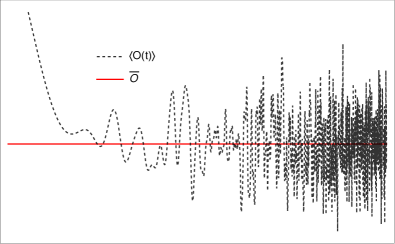
The expectation value of an operator oscillates around its mean value at long times. Consider a Hamiltonian and some operator whose time evolution is studied under this Hamiltonian. This is schematically shown in the Fig. 1. The time evolved operator is given by
| (6) |
The expectation value of this operator in a generic state is given by
| (7) |
The generic state is written as follows in terms of the eigenstates of the Hamiltonian
| (8) |
The expectation value can now be rewritten as
| (9) |
The time-averaged value of this expectation is given as
| (10) | ||||
| (11) |
The integral over gives a . Therefore the final result is
| (12) |
where the second sum is over all for which . So if the mean value is subtracted from , we obtain
| (13) |
where the terms corresponding to degeneracies were dropped. This captures the behavior of the off-diagonal elements of the time-evolved operator.
We evaluate the distribution of the zeros of the function and determine how they are spaced. The moments of the distribution of this spacing can be interpreted as another natural time scale. Note that for random uniform initial state (i.e. are uniform random numbers), this distribution is determined by the level spacing distribution of the Hamiltonian and the off-diagonal elements of the initial operator 444Corresponding to the off-diagonal fluctuation in ETH.
The passage or excursion times are then defined as the interval between the zeros and of the function . There are two passage times which are extracted from this information. The first is the positive passage time which corresponds to being positive in the interval to . The negative passage time corresponds to being negative in the interval to . In this manuscript, we study the statistical distribution of through their mean and variance (and combinations thereof).
III Details of the numerics
In this section, we discuss the details of the numerical computations and present some of the results that are mentioned in the main text.
While determining the passage times, our approach involved first diagonalizing the Hamiltonian (1) to find its eigenvalues and eigenvectors. The next step is determining the coefficients corresponding to the initial state , drawn from a uniform distribution, and the components of the initial operator and then plugging it in the expression (13). Then this function was evaluated numerically by varying in steps of and the values for which were collected. Finally the difference was computed to determine the excursion times. We collected passages.
The results for the short- and long-range networks are discussed in the main text. For the short-range network, the appropriate choice of ergodization time is the ratio of variance and mean of the excursion times as supported by the data showin in Fig. 2. The exponentially larger scale of as compared to suggests that the fluctuations dominate the dynamics. The relative strength of the effect of the fluctuations defines an appropriate time-scale .
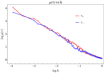
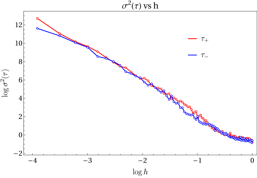
For the long-range network, the mean and variance are of equivalent orders. This suggests that the dynamics is proportionately dominated by the averages as well as the fluctuations. Therefore, one can pick either the mean or variance as the relevant ergodization time . We choose the mean as the ergodization time . This choice is supported by the data shown in Fig. 3. We see that the ratios of the mean and the variance remain of the same order as the integrability breaking parameter is varied. Therefore they do not represent useful timescales that are sensitive to the integrability breaking effect.