Supplemental material for “Quasi-Nambu-Goldstone modes in many-body scar models”

Abstract

From the quasisymmetry-group perspective [Phys. Rev. Lett. 126, 120604 (2021)], we show the universal existence of collective, coherent modes of excitations in many-body scar models in the degenerate limit, where the energy spacing in the scar tower vanishes. The number of these modes, as well as the quantum numbers carried by them, are given, not by the symmetry of the Hamiltonian, but by the quasisymmetry of the scar tower: hence the name quasi-Nambu-Goldstone modes. Based on this, we draw a concrete analogy between the paradigm of spontaneous symmetry breaking and the many-body scar physics in the degenerate limit.

I Introduction

The theory of spontaneous symmetry breaking is one of the underpinning pillars of condensed matter physics. It states that the macroscopic ground state at sufficiently low temperature usually develops an “order”, so that the ordered state, also called the symmetry-broken state, has less symmetry compared with that of the underlying Hamiltonian. An example is the ferromagnetic state developed from a Heisenberg model Heisenberg (1928): while the Hamiltonian has full spin SU(2) symmetry, the ferromagnetic state only retains spin U(1) symmetry, corresponding to the rotation along the ordered moments. Generally speaking, the symmetry $G$ of a Hamiltonian may break down to a lower symmetry $H\subset{G}$ in the ground state of the same Hamiltonian, and the quotient space $Q\equiv{G/H}$ describes the orientation of the order parameter. In the example, $G=\mathrm{SU(2)}$, $H=\mathrm{U(1)}$, and $Q=G/H=S^{2}$ is a sphere of unit vectors, where $\mathbf{v}\in{Q}$ denotes a possible direction of magnetization. One key observation is that while the ground state lowers the symmetry, the low-lying modes of collective excitations Nambu and Jona-Lasinio (1961); Goldstone et al. (1962); Nambu (2009) over the ground state “recover” some of the broken symmetry. These modes correspond to global rotations of the order parameter from one vector $\mathbf{v}\in{Q}$ to another vector $\mathbf{v}^{\prime}$. In the absence of long-range interactions, even if these rotations have small momenta, that is, some slow spatial modulation, the modes remain coherent and continue to zero energy as the momentum goes to zero. These are the Nambu-Goldstone modes (NGM), of which phonons and magnons are typical examples.

Recently, in a Rydberg-atom experiment Bernien et al. (2017), quasi-periodic dynamics in certain observables was observed in the time evolution of a product state having finite energy density. Independently, theorists discovered in the Affleck-Kennedy-Lieb-Tasaki (AKLT) model Affleck et al. (1987) a tower of exact eigenstates having equal energy spacing Moudgalya et al. (2018a). The phenomenon observed in Ref. Bernien et al. (2017) was termed the quantum-many-body scar Turner et al. (2018a) and reproduced in simplified spin models Turner et al. (2018b); Ho et al. (2019); Choi et al. (2019); Lin and Motrunich (2019); Bull et al. (2020); Khemani et al. (2019); Michailidis et al. (2020); Turner et al. (2021); Iadecola et al. (2019); Pan and Zhai (2022) that possess nearly-equally-spaced eigenstates. The tower of states in the AKLT model was also related to QMBS Moudgalya et al. (2018b); Mark et al. (2020), and similar towers were discovered in various spin and fermion models known as the exact scar models Moudgalya et al. (2020a); Shiraishi (2019); Mark and Motrunich (2020); Moudgalya et al. (2020b); Schecter and Iadecola (2019); Chattopadhyay et al. (2020); Shibata et al. (2020); Yang et al. (2020); Iadecola and Schecter (2020); Wildeboer et al. (2022); Langlett et al. (2022); Bull et al. (2019); Hudomal et al. (2020); van Voorden et al. (2020); Iversen et al. (2024); Serbyn et al. (2021); Moudgalya et al. (2022); Chandran et al. (2023). In terms of the energy spectrum, exact scar dynamics corresponds to the existence of a tower of eigenstates, called the scar tower, that has equal energy spacing $hT^{-1}$ buried in the middle of a non-integrable spectrum. In Refs. Ren et al. (2021), it is shown that many scar towers can be unified under a group theoretic framework (see also Refs. O’Dea et al. (2020); Pakrouski et al. (2020, 2021); Sun et al. (2023)), where the tower of states form a representation of a group $\tilde{G}$ that is larger than the symmetry of the Hamiltonian $G$. Operations in $\tilde{G}$ in general do not preserve the Hamiltonian, but preserve the scar tower, and if $\tilde{G}$ is a Lie group, the equal energy spacing can be easily created by adding a constant external field coupled to any generator of $\tilde{G}$. In Ref. Ren et al. (2021), $\tilde{G}$ is called the quasisymmetry group, and a routine is proposed to generate model Hamiltonians for nearly all known scar towers Ren et al. (2021); O’Dea et al. (2020).

Inspired by the recent proposal of the asymptotic scar in the XY-model Gotta et al. (2023); Moudgalya and Motrunich (2023); Kunimi et al. (2024), in this Letter, we establish the general existence of modes of collective excitations in exact bosonic scar models, and relate their defining properties, such as the number of modes and the quantum numbers they can transport, to the quasisymmetry group $\tilde{G}$. This is illustrated using two examples, the ferromagnetic scar model and the AKLT scar model in the main text, then proved for any scar model having an arbitrary $\tilde{G}$ in Appendix A in the degenerate limit. Here the degenerate limit is where the energy spacing vanishes, and the entire scar tower becomes a degenerate-energy subspace. We call these collective modes the quasi-Nambu-Goldstone modes (qNGM), based on the following similarities to the type-B Watanabe and Murayama (2012, 2014); Watanabe (2020); Herzog-Arbeitman et al. (2022) NGM appearing in ferromagnetism: (i) the number of qNGM is the same as the rank of the quasisymmetry group $\tilde{G}$, and the number of type-B NGM is the rank of the symmetry group $G$; (ii) the lifetime $\tau\rightarrow\infty$ as the momentum of the mode $q\rightarrow 0$; and (iii), each qNGM carries the charge of $\tilde{G}$, and each NGM carries that of $G$. There are also key differences: (i) the dispersion of qNGM near the zero momentum is linear, while that of type-B NGM is quadratic; (ii) at $t\gg\tau$, the excitations decay, and the system returns to the ground state in the case of NGM, but to chaotic, thermal states in the case of qNGM.

II qNGM in the ferromagnetic scar model

There are many scar spin models, with the spin-1 XY model serving as a prominent example. In these models, the scar space, up to certain onsite unitary transformations, consists of ferromagnetic (FM) states. These states are parameterized by spherical coordinates:

$$|\text{FM}_{\theta,\phi}\rangle=\includegraphics[width=43.36464pt,valign={c}]{pics/spin-typical}\otimes\cdots\otimes\includegraphics[width=43.36464pt,valign={c}]{pics/spin-typical}.$$ (1)

For a spin-$s$ model of $N$ sites, the scar space $\mathcal{H}_{\mathrm{SO(3)}}=\{|\text{FM}_{\theta,\phi}\rangle|\forall\theta,\phi\}$ form an $S=Ns$ irreducible representation of the quasisymmetry group $\tilde{G}=\mathrm{SO(3)}$, invariant under spin rotation. To be concrete, we consider the following Hamiltonian

$$\hat{H}=\sum_{j=1}^{N}\left[J\hat{\mathbf{s}}_{j}\cdot\hat{\mathbf{s}}_{j+1}-D_{1}(\hat{\mathbf{s}}_{j}\times\hat{\mathbf{s}}_{j+1})_{z}-D_{2}(\hat{\mathbf{s}}_{j}\times\hat{\mathbf{s}}_{j+2})_{x}\right],$$ (2)

where $\hat{\mathbf{s}}_{i}$’s are spin-$s$ operators, and the periodic boundary condition is assumed here and after. Here the $D_{1,2}$ terms break the spin conservation of any component, and introduce “frustration” to the model. Here “frustration” means that the scar states, being eigenstates of $\hat{H}$, are not eigenstates of certain individual terms in $\hat{H}$. One may intuit that $|\text{FM}_{\theta,\phi}\rangle$’s are eigenstates: (i) each inner product takes the maximum value, and (ii) each cross product vanishes as all spins are parallel. This argument is helpful and the conclusion correct, albeit that (ii) is incorrect. (The readers are referred to Appendix B for the rigorous proof.)

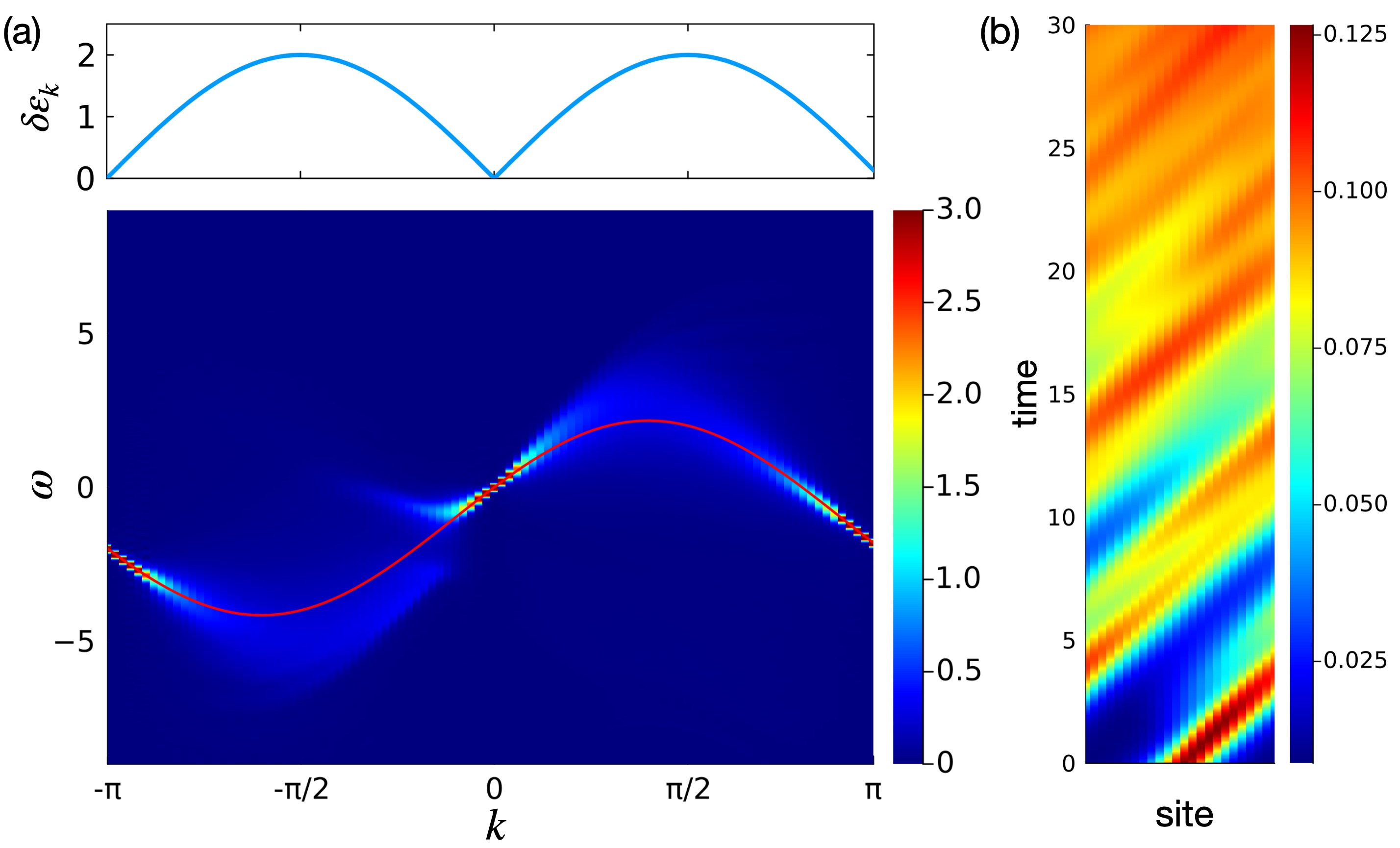
Figure 1: Spin-1/2 ferromagnetic scar model. (a) Bottom: Spectral function $A(k,\omega)$ of a spin-1/2 chain with parameters ($J=1,D_{1}=3,D_{2}=2$), computed utilizing the MPS-based Chebyshev series expansion method Holzner et al. (2011). The system size is $L=100$, and the Chebyshev vectors are approximated by a bond dimension of $\chi=30$ MPSs. We numerically evaluate the Chebyshev series up to order $200$. In presenting the result, we cut off values exceeding $3.0$. The red line denotes the “band” $\varepsilon_{k}$. Top: Energy variance $\delta\varepsilon_{k}$ of $|k\rangle$. Note that in this model there is a vanishing variance at $k=\pi$, which is accidental (see Appendix B). This zero will be absent by adding more terms. (b) Simulation of many-body evolution from a coherent wave-packet on spin-1/2 chain with size $L=24$. To show a long coherent time, we choose the parameters ($J=1,D_{1}=3,D_{2}=0.5$). The heatmap shows the local expectation of the magnon density $n_{j}=\langle\hat{s}_{j}^{z}\rangle+1/2$.

An analogy is observed between the scar model and the FM Heisenberg model $\hat{H}^{\prime}=\sum_{j}J\hat{\mathbf{s}}_{j}\cdot\hat{\mathbf{s}}_{j+1}$ ($J<0$), as both share the FM manifold $\mathcal{H}_{\mathrm{SO(3)}}$ as their scar space or ground state space, respectively. The generators of the SO(3) symmetry play analogous roles in both scenarios: in the scar context, they act as ladder operators, generating the tower states; whereas, in the ground state symmetry-breaking case, they correspond to the NGM. Notably, the NGMs are not confined to the fixed momentum $k_{0}$ determined by the group generator (for the ferromagnetic scar, the homogeneity means $k_{0}=0$); small spatial modulation also yields small energies.

From SO(3) symmetry, we pick without loss of generality the all-down state $|\text{FM}_{\pi,0}\rangle\equiv\left|\Downarrow\right\rangle$ as the symmetry breaking ground state. An NGM with momentum $k$ is generated by the magnon operator:

$$\hat{a}^{\dagger}_{k}=\frac{1}{\sqrt{N}}\sum_{j}\hat{s}^{+}_{j}\exp(ikj).$$ (3)

The single magnon states $|k\rangle\equiv\hat{a}^{\dagger}_{k}\left|\Downarrow\right\rangle$ exhibit a dispersion $\varepsilon_{k}=sJk^{2}$, vanishing as $k\rightarrow 0$. The properties of $|k\rangle$ become evident when examining the spectral function:

$$A(k,\omega)=\mathrm{Im}\int\frac{dt}{i\pi}e^{i\omega{t}}\left\langle\Downarrow\right|\Theta(t)[\hat{a}_{k}(t),\hat{a}^{\dagger}_{k}]\left|\Downarrow\right\rangle.$$ (4)

The NGM in the Heisenberg model $\hat{H}^{\prime}$ is evident as a sharp coherent signal detectable by neutron scattering experiments Ewings et al. (2010); Chisnell et al. (2015).

When $\hat{H}^{\prime}$ undergoes a sudden global quench to the scar Hamiltonian Eq.(2), the original ground state $\left|\Downarrow\right\rangle$ becomes a scar initial state showing revival dynamics in the presence of a transverse field Ren et al. (2021); O’Dea et al. (2020). This property is encoded in the same spectral function Eq.(4), despite the change in the Hamiltonian. The gaplessness of the NGM is governed by symmetry and locality, which are retained in the scar system, rendering $|k\rangle$ significant. Indeed, Fig.1(a) illustrates a linear dispersion and vanishing energy variance as $k\rightarrow 0$. The exact expressions for the energy expectation and variance can be obtained (See Appendix B for the proof):

$$\varepsilon_{k} \equiv \langle{k}|\hat{H}-E_{0}|k\rangle=2sD_{1}k+O(k^{2}),$$ (5)

$$\delta\varepsilon_{k} \equiv \sqrt{\langle{k}|(\hat{H}-E_{0})^{2}|k\rangle-\varepsilon_{k}^{2}}=\sqrt{2s}|D_{2}k|+O(k^{2}).$$

The linear dispersion and vanishing energy variance facilitate the effective transport of quantum numbers. Consider a Gaussian wave packet constructed from $|k\rangle$’s, representing a quasiparticle with momentum $k=0$ and position $x=x_{0}$:

$$|x_{0}\rangle=\int{dp}\exp\left(ipx_{0}-\frac{p^{2}}{2\delta{k}^{2}}\right)|p\rangle.$$ (6)

From Eq.(5), we find that this wave packet is a coherent quasiparticle with lifetime $\tau=|D_{2}|^{-1}\delta{k}^{-1}$, transporting an integer spin $\delta{S}_{z}=\hbar$ along the chain with velocity $v=2sD_{1}$. Fig.1(b) illustrates this coherent propagation using the model parameters provided in the caption. It is noteworthy that as $S_{z}$ is not conserved in $H$, the quantum number transported by the quasi-magnon is not related to the symmetry group $G$, but rather the quasi-symmetry group $\tilde{G}$.

We remark here that the scar initial state need not necessarily be an FM state; rather, it can possess arbitrary order, provided it is parameterized by a Lie group. An example of such a configuration frequently encountered is a “$\pi$-ferromagnetic” spin configuration:

$$|\pi\text{FM}_{\theta,\phi}\rangle=\includegraphics[width=43.36464pt,valign={c}]{pics/spin-typical-a}\otimes\includegraphics[width=43.36464pt,valign={c}]{pics/spin-typical-b}\otimes\cdots,$$ (7)

where the spin configuration consists of even-odd spins that differ by a $\pi$-rotation around the $z$-axis. The symmetric space spanned by $|\pi\text{FM}_{\theta,\phi}\rangle$ also possesses SO(3) symmetry, but the definition of spin rotation differs, with the generator being $\{\hat{s}^{x},\hat{s}^{y},\hat{s}^{z}\}$ on the odd sites while $\{-\hat{s}^{x},-\hat{s}^{y},\hat{s}^{z}\}$ on the even sites.

III qNGM in the AKLT scar model

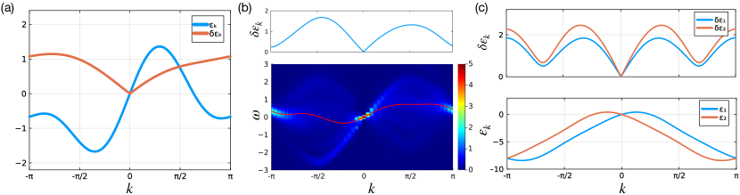
Figure 2: (a)(b) Illustrations of two types of qNGMs for the generalized AKLT model defined in Eq.(14). (c) Depiction of the SU(3) scar model, detailed in Appendix F.1. (a) The energy expectation and variance for the z-qNGM state $|k,x\rangle$. (b) Bottom: Spectral function $\tilde{A}(k,\omega)$ of the x-qNGM for the generalized AKLT model. The computation employs a Chebyshev expansion for an $L=50$ system with a maximum bond dimension $\chi=30$, and the Chebyshev series is calculated up to order $n=100$. The red line represents the dispersion of the energy expectation $\varepsilon_{k}$. Top: Energy variance $\delta\varepsilon_{k}$ of the x-qNGM. Note that at $k\approx\pi$, there seems to be a coherent mode, but the energy variance is always positive. (c) Bottom: Energy expectation of two modes in the SU(3) scar model. Top: Energy variance of two modes.

In the context of FM scar model, the qNGM emerges through spatial modulation in the symmetry generator $\hat{a}^{\dagger}$. However, most exact scar spaces do not have a clear symmetry structure, and the scar initial states are not product states as in the previous case, but matrix-product states Fannes et al. (1992); D. Perez-Garcia (2007), of which the AKLT model is a prime example.

Consider the Hamiltonian

$$\hat{H}_{\text{AKLT}}=\sum_{j}\frac{J}{2}\left[\hat{\mathbf{l}}_{j}\cdot\hat{\mathbf{l}}_{j+1}+\frac{1}{3}(\hat{\mathbf{l}}_{j}\cdot\hat{\mathbf{l}}_{j+1})^{2}\right]-h\hat{l}^{z}_{j},$$ (8)

where $\hat{\mathbf{l}}_{j}$ is the spin-1 operator at site $j$. In Ref. Moudgalya et al. (2018a), the authors discovered a scar tower in Eq.(8), stemming from the ground state $|\text{AKLT}\rangle$, and generated by a “one-way ladder” $\hat{Q}^{\dagger}\equiv\sum_{j}(-1)^{j}(\hat{l}^{+})^{2}$. This ladder creates a tower of scar states by $|n+1\rangle=\hat{Q}^{\dagger}|n\rangle$, but $\hat{Q}|n+1\rangle\neq|n\rangle$, precluding the formation of a symmetry sector. The energy spacing within the scar tower is $\Delta{E}=2(J-h)$. Setting $J=h$ renders the scar tower degenerate.

Although lacking an apparent symmetry structure, Ref. Ren et al. (2022) regards the degenerate scar space as a “deformed” SO(3)-symmetric space, constructed via a two-step process involving two Hilbert spaces: the “prototype space” and the physical space, denoted by the subscripts on kets. In this specific example, the prototype space comprises a chain of $N$ $s=1/2$ spins, while the physical space comprises a chain of $l=1$ spins. The scar initial state takes the form: $|\Psi_{\theta,\phi}\rangle_{\text{phy}}=\hat{W}|\pi\text{FM}_{\theta,\phi}\rangle$, where the operator $\hat{W}$, termed the deforming operator, is a matrix product operator Pirvu et al. (2010); Chan et al. (2016) (MPO) mapping the prototype space to the physical one under periodic boundary conditions. (PBC). The deformed state $|\Psi_{\theta,\phi}\rangle_{\text{phy}}$ represents a PBC MPS Fannes et al. (1992); D. Perez-Garcia (2007) also parameterized by $\theta$ and $\phi$, graphically represented as:

$$|\Psi_{\theta,\phi}\rangle_{\text{phy}}=\includegraphics[width=216.81pt,valign={c}]{pics/dMPS},$$ (9)

where the deforming operator is described by a single four-leg tensor $W^{ls;\alpha\beta}$, with $s=\uparrow,\downarrow$ contracting with the spin index in the prototype space, $l=1,0,-1$ representing the spin index in the physical space, and $\alpha,\beta$ denoting the auxiliary legs encoding entanglement. For scar dynamics to occur, an additional term is necessary to generate equally spaced energy levels within the tower. This implies that the physical tower must retain at least one U(1) symmetry, represented by:

$$\hat{W}\exp(-i\hat{S}^{z}\theta)|\psi\rangle_{\text{pro}}=\exp(-2i\hat{L}^{z}\theta)\hat{W}|\psi\rangle_{\text{pro}}.$$ (10)

Ref. Ren et al. (2022) elucidates that for the AKLT scar space, $W^{ls;\alpha\beta}$ takes the form:

$$W^{1\downarrow}=\sigma^{+},\quad W^{0\downarrow}=-\frac{\sigma^{z}}{\sqrt{2}},\quad W^{-1\downarrow}=-\sigma^{-},$$ (11)

$$W^{1\uparrow}=-\sigma^{-},\quad W^{0\uparrow}=W^{-1\uparrow}=0.$$

Despite that $\hat{W}$ breaks the spin rotation symmetry in the physical space, the hidden symmetry generators in the prototype space enable the extension of the qNGM theorem to more general scenarios. For the general theorem and proof, please refer to the Appendix C.

Due to the existence of U(1) quasisymmetry, the spin-$z$ rotation holds particular significance, leading to two distinct types of qNGMs, termed the $z$-qNGM and the $x$-qNGM. The $z$-qNGM originates from the physical state:

$$|\Psi_{\pi,0}\rangle_{\text{phy}}=\hat{W}\left[\includegraphics[width=30.35657pt,valign={c}]{pics/spin-down}\otimes\includegraphics[width=30.35657pt,valign={c}]{pics/spin-down}\otimes\cdots\right].$$ (12)

Utilizing the hidden symmetry within the prototype space, we define the $z$-qNGM as:

$$|k,z\rangle=\hat{W}\left[\hat{S}_{\pi+k}^{+}\left|\downarrow\cdots\downarrow\right\rangle_{\text{pro}}\right].$$ (13)

Notably, when $k=0$, this state precisely corresponds to the first excited state in the AKLT scar tower. Hence, the $z$-qNGM takes the form of an AKLT tower state generated by a spatially modulated ladder operator $\hat{Q}^{+}$. Fig.2(a) illustrates the energy expectation and variance for $|k,z\rangle$. It is worth mentioning that in the figure, the computation is actually performed utilizing the generalized AKLT model:

$$\hat{H}=\hat{H}_{\text{AKLT}}+\hat{V},$$ (14)

where $\hat{V}$ represents a frustrated term preserving the AKLT tower while introducing finite velocity to qNGMs. The precise form of $\hat{V}$ is given in Appendix D.

While $z$-qNGMs are simple to construct and characterize, they are difficult to obtain from a practical point of view. In the prototype space, all qNGMs are created by acting $\hat{s}^{+}_{k}$ to $\left|\Downarrow\right\rangle_{\text{pro}}$; but in the physical space, the ladder operators do not in general exist. (They do luckily exist in the specific example of AKLT, but not in more general scar towers.) Hence, we shift our focus to qNGMs originating from the scar initial state

$$|\Psi_{\frac{\pi}{2},0}\rangle_{\text{phy}}=\hat{W}\left[\includegraphics[width=30.35657pt,valign={c}]{pics/spin-front}\otimes\includegraphics[width=30.35657pt,valign={c}]{pics/spin-back}\otimes\cdots\right],$$ (15)

from which the qNGM can be locally generated. Leveraging the U(1) quasisymmetry of the scar space, let $\hat{L}^{z}_{k}=\sum_{j}{e}^{ikj}\hat{l}^{z}_{j}$, and we define the $x$-qNGM as:

$$|k,x\rangle\equiv\hat{L}^{z}_{k}|\Psi_{\frac{\pi}{2},0}\rangle_{\text{phy}}.$$ (16)

Since it can be locally generated, $|k,x\rangle$ proves more relevant for potential experimental detection. In Fig.2(b), we present both the spectral function

$$\tilde{A}(k,\omega)=\operatorname{Im}\int\frac{dt}{i\pi}e^{i\omega t}\langle\Psi_{\frac{\pi}{2},0}|\Theta(t)[\hat{L}^{z}_{-k}(t),\hat{L}^{z}_{k}]|\Psi_{\frac{\pi}{2},0}\rangle,$$ (17)

and $(\varepsilon_{k},\delta\varepsilon_{k})$, revealing a nearly coherent mode near $k=0$.

In addition to the AKLT scar mode, Appendix E investigates qNGMs of other scar models featuring deformed symmetric spaces. These include the Rydberg-blockaded scar model Yang et al. (2020); Iadecola and Schecter (2020), the Onsager scar model Shibata et al. (2020), and an additional scar tower in the spin-1 XY model Schecter and Iadecola (2019); Chattopadhyay et al. (2020). These findings underscore the universality of qNGM existence in scar models.

IV General results and remarks

Using two examples of the FM tower and the AKLT tower, we illustrate the ubiquitous existence of quasi-Nambu-Goldstone modes in quantum many-body scar models. They are finite-momentum $k\neq 0$, low-entanglement states having linear dispersion and infinite lifetime as $k\rightarrow 0$. To be specific, a wave packet having width $\delta{k}$ in momentum has lifetime $\tau\propto\delta{k}^{-1}$. (They become the tower eigenstates at $k=0$.) In both examples, the scar tower has the SU(2) quasisymmetry or deformed symmetry, but more complicated scar towers may be similarly considered. In Appendix F.1, we show that two branches of qNGM exist in an SU(3)-scar model. (See Fig.2(c) for energy expectation and variance of two qNGMs.) Generally, the number of qNGM equals the rank of the underlying quasisymmetry (deformed symmetry), and the dynamics of those qNGM is described by a multi-band Hamiltonian.

Like Nambu-Goldstone modes, qNGM can be excited by local fields from a tower state, and they transport quantum numbers. But the quantum numbers are those of the quasisymmetry, instead of the symmetry, of the Hamiltonian. Unlike their low-energy counterpart, qNGM in energy are located within a continuum of thermal states, and will relax into those states long after their lifetime (see Fig.1(b)), since qNGMs are superpositions of thermal eigenstates (see Appendix D and G).

Moreover, the principle of qNGMs from quasisymmetry extends beyond exact scar models to encompass the PXP model, which exhibits a special (approximate) SU(2) quasisymmetry Turner et al. (2018a, b). Within this framework, we can define generalized qNGMs. As detailed in Appendix G, we delve into the properties of PXP qNGMs by examining both the original PXP model Turner et al. (2018a, b) and the deformed PXP model Choi et al. (2019). Through numerical simulation, we confirm that these modes also exhibit approximate revival dynamics. Notably, for the approximate quantum many-body scars, the gradual thermalization of the small-$k$ qNGMs becomes indistinguishable from the inherent thermalization dynamics of the PXP model. Consequently, the qNGM emerges as an interesting initial state for scar dynamics: it dynamically resembles $\mathbb{Z}_{2}$ evolution, yet its spectrum primarily comprises thermal states rather than scar states.

Appendix A Quasi-Nambu-Goldestone Theorem

In this section, we present a formal proof of the quasi-Nambu-Goldstone theorem, which predicts the existence of an asymptotic long-live mode associated with quasisymmetry. To enhance clarity and conciseness, we first review the basis framework of the quasisymmetry framework Ren et al. (2021) before enunciating the theorem.

A.1 Quasisymmetry and quasi-Nambu-Goldstone modes

In this work, we assume the symmetry to be non-Abelian Lie groups, thus possessing high-dimensional irreducible representation. The generators of a rank-$n$ Lie group, when expressed in the Cartan-Weyl basis, consist of $n$ pairs of ladder operators and $n$ mutually commuting operators forming the Cartan subalgebra.

The quasisymmetry framework involves the following elements:

• a product anchor state: $|\Psi_{e}\rangle=|\psi_{e}\rangle^{\otimes N}$;

• a quasisymmetry group $\tilde{G}$ as a onsite symmetry action: $|\Psi_{g}\rangle=\hat{U}_{g}|\Psi_{e}\rangle=e^{i\theta_{a}\hat{Q}_{a}}|\Psi_{e}\rangle$;

• a quasisymmetric Hamiltonian $\hat{H}$ degenerate in the quasisymmetry subspace $\mathcal{H}_{\tilde{G}}\equiv\operatorname{span}\{\hat{U}_{g}|\Psi_{e}\rangle|\forall g\in\tilde{G}\}$;

• a spectrum splitting term $\hat{H}_{z}=\sum_{j=1}^{N}\hat{q}_{j}^{z}$ chosen from the generators of the Lie algebra.

We also assume that the anchor state is in the highest-weight representation of $\tilde{G}$. In terms of local state $|\psi_{e}\rangle$, this means $|\psi_{e}\rangle$ is the ground state of a local group generator, denoted as $\hat{q}^{z}$. The product state $|\Psi_{e}\rangle$ is automatically the eigenstate of $\hat{Q}^{z}=\sum_{j}\hat{q}_{j}^{z}$, and the eigenvalue (corresponding to the weight in mathematics) is maximal.

For a Hamiltonian with quasisymmetry $\tilde{G}$, on top of the anchor state $|\Psi_{e}\rangle$, the state

$$\hat{Q}^{+}|\Psi_{e}\rangle=\sum_{j=1}^{N}\hat{q}_{j}^{+}|\Psi_{e}\rangle$$ (18)

is also the eigenstate in the scar space. Note that we assume the quasisymmetry generator has zero momentum, although other momenta are generally possible, with the generator expressed as

$$\hat{Q}^{+}_{k}=\sum_{j=1}^{N}e^{ikj}\hat{q}_{j}^{+}$$ (19)

in the general scenario. Nonetheless, we can always apply a unitary transformation

$$\hat{U}=\bigotimes_{j=1}^{N}\exp\left(-ikj\hat{q}_{j}^{z}\right),\quad\hat{U}\hat{Q}_{k}^{+}\hat{U}^{\dagger}=\hat{Q}^{+},$$ (20)

where $[\hat{q}_{j}^{z},\hat{q}_{j}^{+}]=\hat{q}_{j}^{+}$, to shift the momentum to zero without breaking the translational symmetry of the local Hamiltonian, and the following theorem remains valid. Hence, we will focus on the case where $k=0$.

The quasi-Goldstone mode is defined as

$$|k\rangle\equiv\frac{1}{\mathcal{N}_{k}}\hat{Q}_{k}^{+}|\Psi_{e}\rangle=\frac{1}{\mathcal{N}_{k}}\sum_{j}e^{ikj}\hat{q}_{j}^{+}|\Psi_{e}\rangle,$$ (21)

where $k$ is a nonzero crystal momentum. In the forthcoming sections, we demonstrate that any scar model governed by the quasisymmetry group $\tilde{G}$ possesses a quasi-Goldstone mode, characterized by an energy variance that converges to zero as $k$ approaches zero.

A.2 Quasi-Nambu-Golstone theorem

Theorem 1 (Quasi-Nambu-Golstone theorem).

For a translational invariant local Hamiltonian $\hat{H}$ with quasisymmetry $\tilde{G}$ and ladder operator $\hat{Q}$. The energy expectation

$$\varepsilon_{k}\equiv E_{k}-E_{0}=\langle k|\hat{H}|k\rangle-\langle 0|\hat{H}|0\rangle$$

and the energy variance

$$\delta\varepsilon^{2}_{k}\equiv\langle k|\left(\hat{H}-\langle k|\hat{H}|k\rangle\right)^{2}|k\rangle$$

is a continuous function of $k$, consequently converging to zero as $k$ approaches zero.

Remark.

The original Goldstone theorem is formulated within the context of field theory, assuming the dispersion $\varepsilon_{k}$ as a continuous function of $k$, with the gaplessness being evident due to $\varepsilon_{k=0}=0$. In contrast, our approach in this study begins with a more concrete lattice model, abstaining from presuming the existence of a well-defined field theory. For a system comprising $N$ sites, the normalization $\mathcal{N}(N,k)$, energy $\varepsilon(N,k)$, and energy variance $\delta\varepsilon^{2}(N,k)$ are dependent on both $N$ and $k$. We shall establish that, as the system approaches the thermodynamic limit with $N\rightarrow\infty$, the resulting energy $\varepsilon_{k}$ and variance $\delta\varepsilon^{2}_{k}$ become well-defined and continuous functions of $k$.

Lemma 1 (Normalization).

The normalization factor $\mathcal{N}_{k}$ of the quasi-Goldstone mode $|k\rangle$ is independent of $k$, and is proportional to $\sqrt{N}$:

$$\mathcal{N}_{k}=\mathcal{N}=\sqrt{N}\Delta q,$$

where $\Delta q$ is determined by:

$$\Delta q^{2}=\langle\psi_{e}|\hat{q}^{-}\hat{q}^{+}|\psi_{e}\rangle-|\langle\psi_{e}|\hat{q}^{+}|\psi_{e}\rangle|^{2}.$$

Here $|\psi_{e}\rangle$ is the local state that defines the anchor state, $\hat{q}^{-}=(\hat{q}^{+})^{\dagger}$, and $\hat{q}^{+}$ is the local generator that defines the quasisymmetry action.

Proof.

The inner product $\langle k|k\rangle$ gives:

$$\mathcal{N}^{2}_{k}=\sum_{j}\langle\Psi_{e}|\hat{q}_{j}^{-}\hat{q}_{j}^{+}|\Psi_{e}\rangle+\sum_{j\neq l}e^{ik(j-l)}\langle\Psi_{e}|\hat{q}^{-}_{j}\hat{q}_{l}^{+}|\Psi_{e}\rangle.$$

Since $\Psi_{e}$ is a translational-invariant product state, the expectation $\langle\hat{q}_{j}^{+}\hat{q}_{l}\rangle$ for $j\neq l$ is simply $\langle\hat{q}^{+}\rangle\langle\hat{q}\rangle=|\langle\hat{q}\rangle|^{2}$. Also, for nonzero crystal momentum $k$,

$$\sum_{j,l=1}^{N}e^{ik(l-j)}\langle\hat{q}_{j}^{-}\hat{q}_{l}^{+}\rangle =|\langle\hat{q}^{+}\rangle|^{2}\sum_{j,l=1}^{N}e^{ik(l-j)}=0$$ (22)

$$\quad\Longrightarrow\quad\sum_{j\neq l}e^{ik(j-l)}\langle\hat{q}_{j}^{-}\hat{q}_{l}^{+}\rangle =-\sum_{j}|\langle\hat{q}_{j}^{+}\rangle|^{2}.$$

The normalization thus becomes a finite summation. From the translational invariance, we get a compact expression:

$$\mathcal{N}_{k}^{2} =\sum_{j}\left[\langle\hat{q}_{j}^{-}\hat{q}_{j}^{+}\rangle-|\langle\hat{q}_{j}^{+}\rangle|^{2}\right]$$

$$=N\left(\langle\psi_{e}|\hat{q}^{-}\hat{q}^{+}|\psi_{e}\rangle-\langle\psi_{e}|\hat{q}^{-}|\psi_{e}\rangle\langle\psi_{e}|\hat{q}^{+}|\psi_{e}\rangle\right),$$

and therefore proved the lemma. ∎

Proof of the main theorem.

We assume that the translational invariant Hamiltonian has the form

$$\hat{H}=\sum_{j=1}^{N}\hat{h}_{j},$$ (23)

where $\hat{h}_{j}$ acts nontrivially on the block of sites [$j,\cdots,j+m$].

Energy dispersion: The energy expectation of $|k\rangle$ is

$$\varepsilon_{k} =\frac{1}{\mathcal{N}^{2}}\left(\langle\hat{Q}_{k}^{-}\hat{H}\hat{Q}_{k}^{+}\rangle-\langle\hat{Q}^{-}\hat{H}\hat{Q}^{+}\rangle\right)$$

$$=\frac{1}{\mathcal{N}^{2}}\left(\langle\hat{Q}_{k}^{-}[\hat{H},\hat{Q}_{k}^{+}]\rangle+\langle\hat{Q}_{k}^{-}\hat{Q}_{k}^{+}\hat{H}\rangle-\langle\hat{Q}^{-}\hat{Q}^{+}\hat{H}\rangle\right)$$

$$=\frac{1}{\mathcal{N}^{2}}\langle\hat{Q}_{k}^{-}[\hat{H},\hat{Q}_{k}^{+}]\rangle.$$

We need to show next that $\langle\hat{Q}_{k}^{-}[\hat{H},\hat{Q}_{k}^{+}]\rangle=Nf(k)$ where $f(k)$ is a continuous function. From the locality of the Hamiltonian, the commutator can be reduced to

$$\left[\hat{H},\hat{Q}_{k}^{+}\right] =\sum_{l}\sum_{j}e^{ikj}\left[\hat{h}_{l},\hat{q}_{j}^{+}\right]$$

$$=\sum_{l}e^{ikl}\left(\sum_{j=0}^{m}e^{ikj}\left[\hat{h}_{l},\hat{q}_{l+j}^{+}\right]\right).$$

We can further define an operator

$$\hat{\Phi}_{l}^{+}(k)=\sum_{j=0}^{m}e^{ikj}\left[\hat{h}_{l},\hat{q}_{l+j}^{+}\right]$$ (24)

acting on block $[l,\dots,l+m]$. $\hat{\Phi}_{l}^{+}(k)$ is translational invariant (its action does not depend on $l$), while it depends on momentum $k$. Using this notation, the summation can then be simplified to

$$\varepsilon_{k}= \ \frac{1}{\mathcal{N}^{2}}\sum_{j,l=1}^{N}e^{ik(l-j)}\langle\hat{q}_{j}^{-}\hat{\Phi}_{l}^{+}(k)\rangle$$

$$= \ \frac{1}{\mathcal{N}^{2}}\sum_{l=1}^{N}\left[\sum_{j\in[l,l+m]}e^{ik(l-j)}\langle\hat{q}^{-}_{j}\hat{\Phi}_{l}^{+}(k)\rangle\right.$$

$$\left.+\sum_{j\notin[l,l+m]}e^{ik(l-j)}\langle\hat{q}^{-}_{j}\hat{\Phi}^{+}_{l}(k)\rangle\right].$$

Since the $|\Psi_{e}\rangle$ is a product state, the cluster decomposition always holds whenever $\hat{q}_{j}^{-}$ and $\hat{\Phi}_{l}^{+}(k)$ have no spatial overlap:

$$\sum_{j\notin[l,l+m]}e^{ik(l-j)}\langle\hat{q}^{-}_{j}\hat{\Phi}_{l}^{+}(k)\rangle =\sum_{j\notin[l,l+m]}e^{ik(l-j)}\langle\hat{q}^{-}\rangle\langle\hat{\Phi}_{l}^{+}(k)\rangle$$

$$=-\sum_{j=0}^{m}e^{-ikj}\langle\hat{q}^{-}\rangle\langle\hat{\Phi}^{+}(k)\rangle,$$

where we have use the same summation trick in Eq. (22). Therefore,

$$\varepsilon_{k}=\frac{1}{\Delta q^{2}}\sum_{j=0}^{m}e^{-ikj}\left[\langle\hat{q}^{-}_{j}\hat{\Phi}_{0}^{+}(k)\rangle-\langle\hat{q}^{-}\rangle\langle\hat{\Phi}^{+}(k)\rangle\right].$$ (25)

Since the expression is a finite sum of analytic functions, $\varepsilon_{k}$ is an analytical function of $k$. By definition, $\varepsilon_{k=0}=0$, therefore, $\varepsilon_{k}\rightarrow 0$ when $k\rightarrow 0$. We have proved the first part of the theorem.

Energy variance: The direct calculation of $\delta\varepsilon_{k}^{2}$ gives:

$$\delta\varepsilon_{k}^{2}= \ \frac{1}{\mathcal{N}^{2}}\left\langle\hat{Q}_{k}^{-}(\hat{H}-E_{k})^{2}\hat{Q}_{k}^{+}\right\rangle$$

$$= \ \frac{1}{\mathcal{N}^{2}}\left\langle\hat{Q}_{k}^{-}(\hat{H}-E_{k})\left[\hat{H}-E_{k},\hat{Q}_{k}^{+}\right]\right\rangle$$

$$+\frac{\varepsilon_{k}}{\mathcal{N}}\left\langle\hat{Q}_{k}^{-}(\hat{H}-E_{k})\hat{Q}_{k}^{+}\right\rangle.$$

The second term on the right-hand side vanishes since $\frac{1}{\mathcal{N}}\langle\hat{Q}_{k}^{-}\hat{H}\hat{Q}_{k}^{+}\rangle=E_{k}$. The expression then becomes

$$\delta\varepsilon_{k}^{2}= \ \frac{1}{\mathcal{N}^{2}}\left\langle\hat{Q}_{k}^{-}(\hat{H}-E_{k})\left[\hat{H},\hat{Q}_{k}^{+}\right]\right\rangle$$

$$= \ \frac{1}{\mathcal{N}^{2}}\left\langle\left[\hat{Q}_{k}^{-},\hat{H}-E_{k}\right]\left[\hat{H},\hat{Q}_{k}^{+}\right]\right\rangle$$

$$+\frac{1}{\mathcal{N}^{2}}\left\langle(\hat{H}-E_{k})\hat{Q}_{k}^{-}\left[\hat{H},\hat{Q}_{k}^{+}\right]\right\rangle$$

$$= \ \frac{1}{\mathcal{N}^{2}}\left\langle\left[\hat{H},\hat{Q}_{k}^{+}\right]^{\dagger}\left[\hat{H},\hat{Q}_{k}^{+}\right]\right\rangle-\varepsilon_{k}^{2}.$$

Using the notation of $\hat{\Phi}^{+}(k)$, the commutator is:

$$\left[\hat{H},\hat{Q}_{k}^{+}\right]=\sum_{l}e^{ikl}\hat{\Phi}_{l}^{+}(k).$$

Therefore the energy variance is

$$\delta\varepsilon_{k}^{2}+\varepsilon_{k}^{2}= \ \frac{1}{\mathcal{N}^{2}}\sum_{l=1}^{N}\left[\sum_{j=-m}^{m}e^{-ikj}\langle\hat{\Phi}^{-}_{l+j}\hat{\Phi}_{l}^{+}\rangle\right.$$

$$\left.+\sum_{j\notin[-m,m]}e^{-ikj}\langle\hat{\Phi}^{-}_{l+j}\rangle\langle\hat{\Phi}_{l}^{+}\rangle\right].$$

The disconnected sum becomes

$$\sum_{j\notin[-m,m]}e^{-ikj}\langle\hat{\Phi}^{-}_{l+j}\rangle\langle\hat{\Phi}_{l}^{+}\rangle=-\sum_{j=-m}^{m}e^{-ikj}|\langle\hat{\Phi}^{+}\rangle|^{2}.$$

Therefore,

$$\delta\varepsilon_{k}^{2}=\frac{1}{\Delta q^{2}}\sum_{j=-m}^{m}e^{-ikj}\left[\left\langle\hat{\Phi}^{-}_{i_{0}+j}\hat{\Phi}_{i_{0}}^{+}\right\rangle-|\langle\hat{\Phi}\rangle|^{2}\right]-\varepsilon_{k}^{2}.$$ (26)

Being a finite sum of analytic functions, $\delta\varepsilon_{k}^{2}$ is also analytic. By definition, $\delta\varepsilon_{k=0}^{2}=0$ and $\delta\varepsilon_{k=0}^{2}\geq 0$ for all $k$, the asymptotic behavior can only be:

$$\Delta H^{2}(k)\sim O(k^{2}).$$ (27)

We, therefore, proved the quasi-Goldstone theorem. ∎

A.3 Remarks and corollaries

The quasi-Goldstone theorem only requires the energy dispersion to be gapless, i.e., $\varepsilon_{k\rightarrow 0}\rightarrow 0$. The following corollary further states that, for the quasi-goldstone mode to have nonzero velocity, the Hamiltonian should be frustrated, i.e., the scar state $|\Psi_{g}\rangle$ is not an eigenstate of local term $h_{j}$.

Corollary 1 (Frustration and velocity).

For frustration-free Hamiltonians, the energy expectations $\varepsilon_{k}\propto O(k^{2})$.

Proof.

Without loss of generality, we assume $\langle 0|\hat{H}|0\rangle=0$. In the proof above, the expression for the energy expectation is

$$\varepsilon_{k}=\frac{1}{\mathcal{N}^{2}}\langle\hat{Q}_{k}^{-}H\hat{Q}^{+}_{k}\rangle=\frac{1}{\Delta q^{2}}\sum_{j,l}e^{ik(l-j)}\langle\hat{q}_{j}\hat{h}_{0}\hat{q}^{+}_{l}\rangle.$$

The derivative near $k=0$ is

$$-i\Delta q^{2}\left.\partial_{k}E_{k}\right|_{k=0} =\sum_{j,l}(l-j)\langle\hat{q}_{j}\hat{h}_{0}\hat{q}_{l}^{+}\rangle$$

$$=\sum_{j,l}l\langle\hat{q}_{j}\hat{h}_{0}q_{l}^{+}\rangle-\sum_{j,l}j\langle\hat{q}_{j}\hat{h}_{0}\hat{q}_{l}^{+}\rangle.$$

The right-hand-side vanishes since $\hat{h}\sum_{j}\hat{q}^{+}_{j}|\Psi_{e}\rangle=0$ for frustration-free Hamiltonian. ∎

Our discussion on the quasi-Goldstone mode now is focused on the highest weight state. The conclusion however can be generalized to tower states in the quasisymmetric scar models. Notably, the original asymptotic scar Gotta et al. (2023) in spin-1 XY model is defined on top of a tower state.

Corollary 2.

For the scar tower state taking the form of the standard weight in the Lie algebra representation:

$$|\Psi_{\bm{M}}\rangle=\hat{Q}^{+}_{\bm{\lambda}}\cdots\hat{Q}^{+}_{\bm{\beta}}\hat{Q}^{+}_{\bm{\alpha}}|\Psi_{e}\rangle$$

The state

$$|k,\bm{M}\rangle\equiv\sum_{j=1}^{N}e^{ikj}\hat{q}^{+}_{j}|\Psi_{\bm{M}}\rangle$$

also has the asymptotic behaviors as $|k\rangle$.

Proof.

To prove that $|k,\bm{M}\rangle$ is an asymptotic scar, we only need to check that the untwisted state $|\Psi_{\bm{M}}\rangle$ is

• invariant under permutations;

• has a converged local density matrix.

The permutational invariance implies that the expectation for two non-overlapping operators

$$\langle\Psi_{\bm{M}}|\hat{A}_{i}\hat{B}_{j}|\Psi_{\bm{M}}\rangle$$ (28)

is independent of their position. Therefore, the summation trick Eq. (22) still applies, and we still have Eqs. (25) and (26). The only difference is that the expectation $\langle\cdots\rangle$ is now taken from $|\Psi_{\bm{M}}\rangle$, of which local expectation is size-dependent. However, it can be shown that those states have convergent local density matrices, and therefore the local expectation is well-defined in the thermodynamic limit. ∎

Appendix B Ferromagnetic Scar Model

In this section, we discuss properties of the spin-$s$ chain with Heisenberg and Dzyaloshinskii-Moriya (DM) interactions, described by the Hamiltonian:

$$\hat{H}= \ \sum_{j=1}^{N}[J\hat{\mathbf{s}}_{j}\cdot\hat{\mathbf{s}}_{j+1}-D_{1}(\hat{\mathbf{s}}_{j}\times\hat{\mathbf{s}}_{j+1})_{z}$$ (29)

$$-D_{2}(\hat{\mathbf{s}}_{j}\times\hat{\mathbf{s}}_{j+2})_{x}+h\hat{s}^{z}_{j}].$$

Here, we add an external field to split lift the degeneracy of the scar tower. When $s=1/2$, the Heisenberg term is integrable, while $D_{1}$ and $D_{2}$ terms break the integrability and the conservation of any spin component.

Note that when $h=0$, besides translational symmetry, the model also features a $\mathbb{Z}_{2}$ reflection+spin flip symmetry:

$$\mathcal{P}:\hat{s}^{x/y}_{j}\rightarrow\hat{s}^{x/y}_{N-j},\quad\hat{s}^{z}_{j}\rightarrow-\hat{s}^{z}_{N-j}.$$ (30)

Then in the compatible sector ($k=0$ or $k=\pi$), the symmetry sector shall be further reduced to examine the level statistics. This extra is relieved once we set $h\neq 0$ as it breaks such $\mathbb{Z}_{2}$ symmetry.

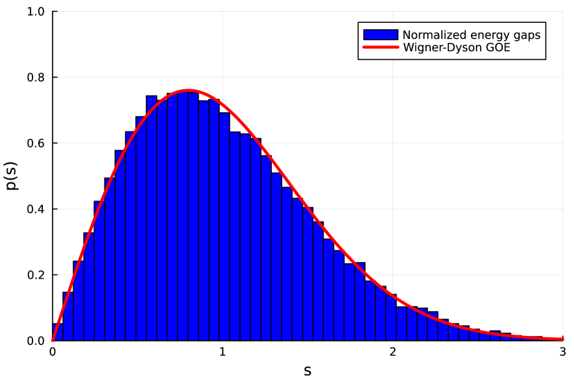
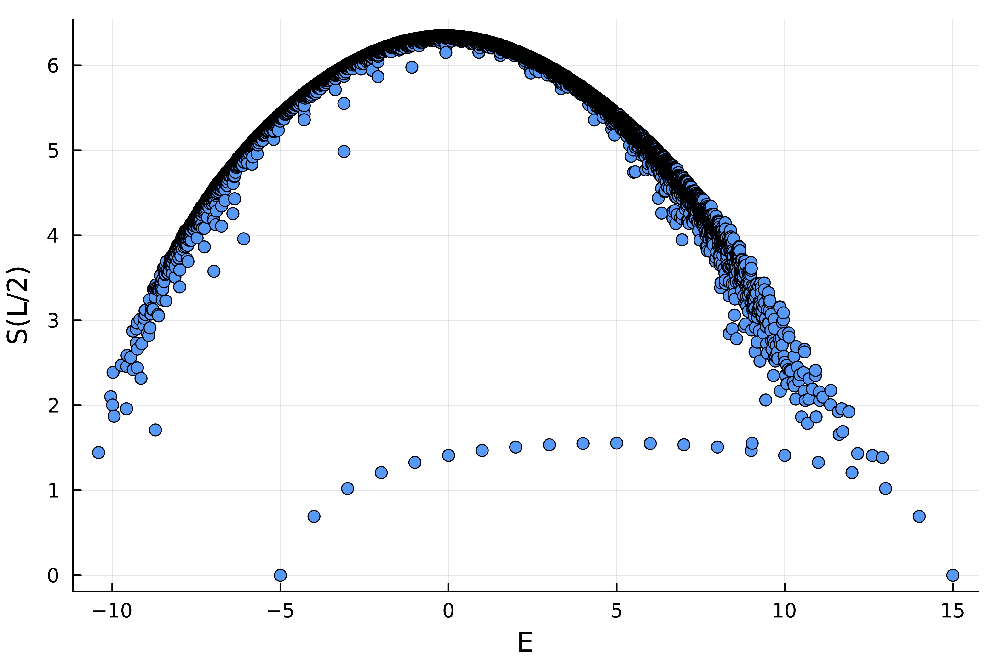
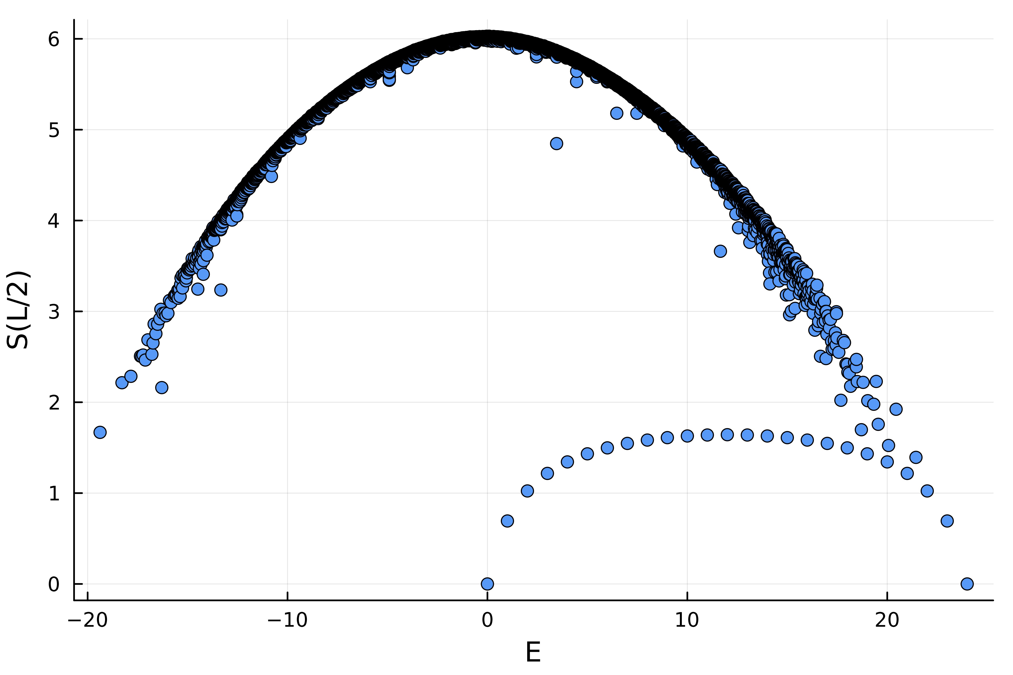
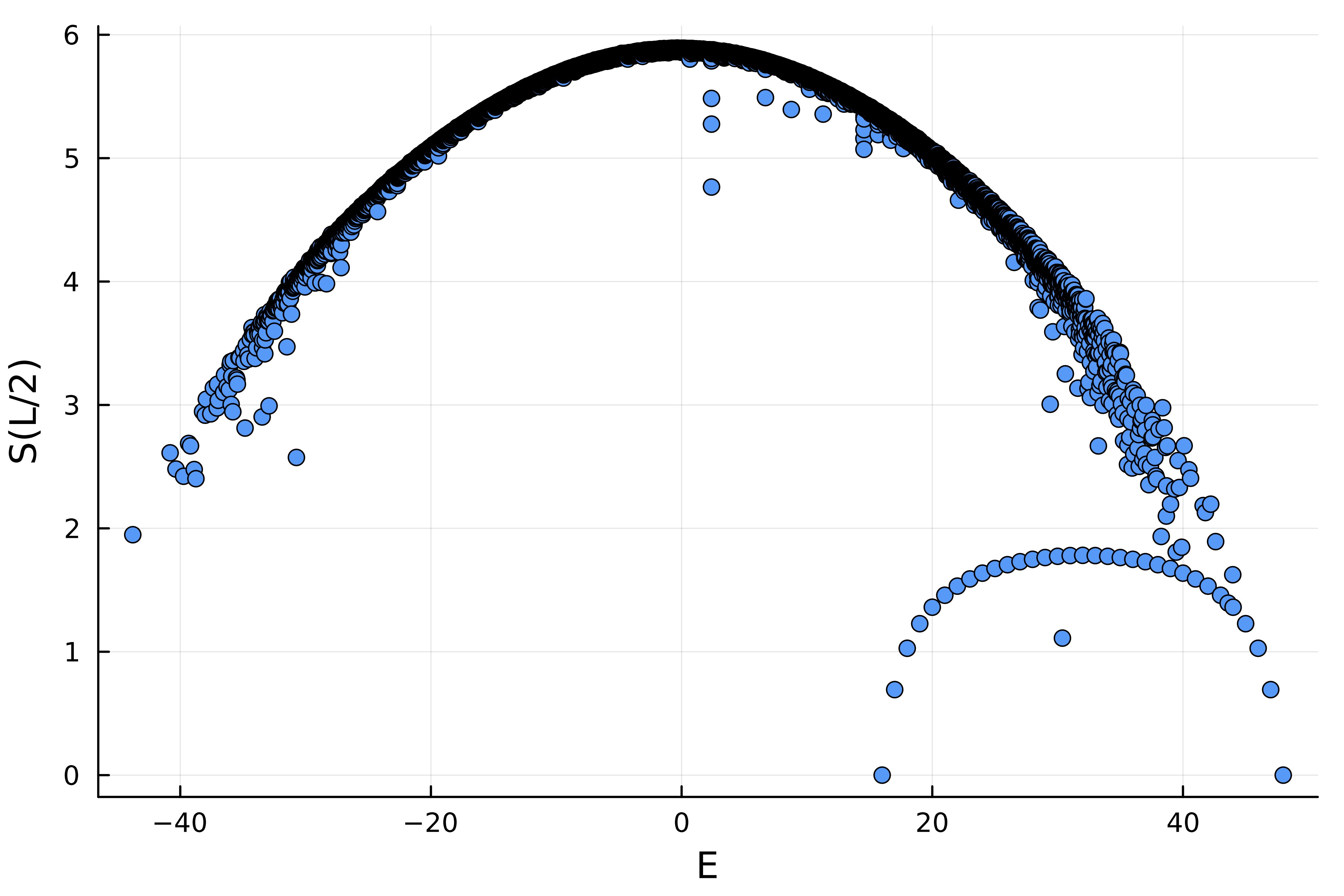
Figure 3: Level statistics and entanglement entropy in ferromagnetic scar models Eq. (29), with $J=1$, $D_{1}=-1/2$, $D_{2}=1/3$, and $h=1$, focusing on the ($k=0$) sector. (a1)(a2) Spectrum of the $L=20$, $s=1/2$ spin chain, with Hilber space dimension $\dim\mathcal{H}=52488$. (b1)(b2) Spectrum of the $L=12$, $s=1$ spin chain, with Hilber space dimension $\dim\mathcal{H}=44368$. (c1)(c2) Spectrum of the $L=8$, $s=2$ spin chain, with Hilber space dimension $\dim\mathcal{H}=48915$. (a1)(b1)(c1) Statistics of energy gaps in the middle half the ($k=0$) sector show Wigner-Dyson GOE form, indicating non-integrability. (a2)(b2)(c2) Entanglement entropy for eigenstates in the ($k=0$) sector reveals scar behavior across different spin values, with tower states displaying notably lower entanglement entropy.

By performing the exact diagonalization on the $k=0$ sectors, we examine the spectrum of the ferromagnetic models and demonstrate numerically that for different choices of $s$, the model in Eq. (29) displays a clear quantum many-body scar phenomenon (see Fig. 3).

B.1 Exact scar tower on spin-$s$ chain

Theorem 2.

The ferromagnetic subspace in the spin-$s$ chain

$$\mathcal{H}_{\text{FM}}\equiv\operatorname{span}\left\{\left.(\hat{S}^{+})^{n}|-s\rangle^{\otimes N}\right|n=0,1,\dots,2sN\right\},$$

is the scar space of the Hamiltonian Eq. (29).

Proof.

The Heisenberg interaction

$$\hat{J}_{d}=\sum_{j=1}^{N}\hat{\mathbf{s}}_{j}\cdot\hat{\mathbf{s}}_{j+d}$$

manifestly has the SO(3) symmetry, and the ferromagnetic is its eigenspace. We will then prove that the Dzyaloshinskii-Moriya type of interaction

$$\hat{\mathbf{D}}_{d}\equiv\sum_{j=1}^{N}\hat{\mathbf{s}}_{j}\times\hat{\mathbf{s}}_{j+d}$$ (31)

will annihilate the spin-$s$ ferromagnetic space $\mathcal{H}_{\text{FM}}$. The first observation is that the vector $(\hat{D}_{d}^{x},\hat{D}_{d}^{y},\hat{D}_{d}^{z})$ form a vector representation of SO(3). The ferromagnetic space is SO(3) invariant. As the result, proofing $\hat{D}^{z}_{d}\mathcal{H}_{\text{FM}}=0$ is enough to show that $\hat{\mathbf{D}}_{d}\mathcal{H}_{\text{FM}}=0$. The $z$-component $\hat{D}^{z}_{d}$ can be expressed as

$$\hat{D}^{z}_{d}=\frac{i}{2}\sum_{j}(\hat{s}_{j}^{+}\hat{s}_{j+d}^{-}-\hat{s}_{j}^{-}\hat{s}_{j+d}^{+}).$$ (32)

It automatically annihilates $|0\rangle$ because of the $\hat{s}^{-}$ operators. What we need to show is that

$$\hat{D}^{z}_{d}|n\rangle=\hat{D}^{z}_{d}(\hat{S}^{+})^{n}|0\rangle=0.$$ (33)

We will need the following commutation relation:

$$\left[\hat{D}^{z}_{d},\hat{S}^{+}\right] =\frac{i}{2}\sum_{j}\left[\hat{s}_{j}^{+}\hat{s}_{j+d}^{-}-\hat{s}_{j}^{-}\hat{s}_{j+d}^{+},\hat{s}_{j}^{+}+\hat{s}_{j+d}^{+}\right]$$ (34)

$$=-i\sum_{j}\hat{s}_{j}^{+}(\hat{s}^{z}_{j+d}-\hat{s}_{j-d}^{z}).$$

Therefore,

$$\left[[\hat{D}^{z}_{d},\hat{S}^{+}],\hat{S}^{+}\right]=0.$$ (35)

Using the commutation relation, Eq. (33) becomes

$$\hat{D}^{z}_{d}|n\rangle =\hat{D}^{z}_{d}\hat{S}^{+}|n-1\rangle$$ (36)

$$=(S^{+})^{n-1}[\hat{D}^{z}_{d},\hat{S}^{+}]|0\rangle+\hat{S}^{+}\hat{D}^{z}_{d}|n-1\rangle.$$

For the first part, since $|0\rangle$ is the eigenstate of all $\hat{s}^{z}$

$$[\hat{D}^{z}_{d},\hat{S}^{+}]|0\rangle=si\sum_{j}(\hat{s}_{j}^{+}-\hat{s}_{j+d}^{+})|0\rangle=0.$$ (37)

Therefore,

$$\hat{D}^{z}_{d}|n\rangle=\hat{S}^{+}\hat{D}^{z}_{d}|n-1\rangle=(\hat{S}^{+})^{n}\hat{D}^{z}_{d}|0\rangle=0.$$ (38)

We therefore proved Eq. (33). Thus $\mathcal{H}_{\text{FM}}$ is the eigenspace of Hamiltonian Eq. (29). ∎

B.2 Energy dispersion and variance

In the following, we always consider the degenerate limit by setting $h=0$. For the ferromagnetic model, the quasisymmetry is SO(3), generated by usual spin generators:

$$\hat{q}^{\pm}=\hat{s}^{\pm},\quad\hat{q}^{z}=\hat{s}^{z}.$$ (39)

The anchor state is the product of polarized states:

$$|\Psi_{e}\rangle=\bigotimes_{j=1}^{N}|\psi_{e}\rangle,\quad|\psi_{e}\rangle=|-s\rangle.$$ (40)

The energy dispersion and variance can be directly calculated using Eq. (25) and Eq. (26). First, we calculate the normalization $\mathcal{N}^{2}=N\Delta q^{2}$, where by definition:

$$\Delta q^{2}=\langle\psi_{e}|\hat{q}^{-}\hat{q}^{+}|\psi_{e}\rangle=\langle\psi_{e}|[\hat{q}^{-},\hat{q}^{+}]|\psi_{e}\rangle=-2\langle\psi_{e}|\hat{q}^{z}|\psi_{e}\rangle=2s.$$

Then we calculate the quantity $\hat{\Phi}_{l}^{+}(k)$:

$$\Phi_{l}^{+}(k)= \ J\sum_{j=1,2}e^{ikj}\left[\hat{h}_{\text{Heisenberg},l},\hat{s}^{+}_{l+j}\right]-D_{1}\sum_{j=1,2}e^{ikj}\left[\hat{h}_{\text{DM-1},l},\hat{s}^{+}_{l+j}\right]-D_{2}\sum_{j=1,3}e^{ikj}\left[\hat{h}_{\text{DM-2},l},\hat{s}^{+}_{l+j}\right]$$

$$= \ J\left[-\hat{s}_{l}^{z}\hat{s}_{l+1}^{x}-e^{ik}\hat{s}_{l}^{x}\hat{s}_{l+1}^{z}-i\hat{s}_{l}^{z}\hat{s}_{l+1}^{y}-ie^{ik}\hat{s}_{l}^{y}\hat{s}_{l+1}^{z}+\hat{s}_{l}^{+}\hat{s}_{l+1}^{z}+e^{ik}\hat{s}_{l}^{z}\hat{s}_{l+1}^{+}\right]$$

$$-D_{1}\left[-\hat{s}_{l}^{z}\hat{s}_{l+1}^{y}-ie^{ik}\hat{s}_{l}^{x}\hat{s}_{l+1}^{z}+i\hat{s}_{l}^{z}\hat{s}_{l+1}^{x}+\hat{s}_{l}^{y}\hat{s}_{l+1}^{z}\right]$$

$$-D_{2}\left[-i\hat{s}_{l}^{z}\hat{s}_{l+2}^{z}+e^{2ik}\hat{s}_{l}^{y}\hat{s}_{l+2}^{+}-\hat{s}_{l}^{+}\hat{s}_{l+2}^{y}+ie^{2ik}\hat{s}_{l}^{z}\hat{s}_{l+2}^{z}\right].$$

Note that in Eq. (25) and Eq. (26), $\hat{\Phi}^{+}(k)$ always acts directly on $|\Psi_{e}\rangle$. Therefore, we can make the following substitution without changing the result:

$$\hat{s}^{x}\simeq\frac{1}{2}\hat{s}^{+},\quad\hat{s}^{y}\simeq-\frac{i}{2}\hat{s}^{+},\quad\hat{s}^{z}\simeq-s.$$ (41)

The operator $\hat{\Phi}_{l}^{+}(k)$ can then be simplified to

$$\Phi_{l}^{+}(k)\simeq -sJ\left[(e^{ik}-1)\hat{s}_{l+1}^{+}+(1-e^{ik})\hat{s}_{l}^{+}\right]+isD_{1}\left[\hat{s}_{l+1}^{+}-e^{ik}\hat{s}_{l}^{+}\right]-i(e^{i2k}-1)D_{2}\left[s^{2}-\frac{1}{2}\hat{s}_{l}^{+}\hat{s}_{l+2}^{+}\right].$$

Now we can compute the dispersion using Eq. (25):

$$\varepsilon_{k} =\frac{1}{2s}\sum_{j}e^{-ikj}\langle\hat{s}^{-}_{j}\hat{\Phi}_{0}^{+}(k)\rangle=\frac{1}{2s}\left[-2s^{2}J(2-e^{-ik}-e^{ik})+i2s^{2}D_{1}\left(e^{-ik}-e^{ik}\right)\right]$$ (42)

$$=2Js\left[\cos k-1\right]+2sD_{1}\sin k.$$

For the energy variance, we can in principle do the calculation using Eq. (26). However, the calculation for this specific case can be significantly simplified. The simplification essentially comes from the fact that $|k\rangle$ is the eigenstate of the scar Hamiltonian when $D_{2}=0$, since the symmetry sector ($S^{z}_{\text{tot}}=-Ns+1,k=k$) is one-dimension. We thus expect the variance to be solely controlled by $D_{2}$. For concrete proof of the above statement, we first note that in Eq. (26), the central quantity to calculate is the expectation $\langle\hat{\Phi}^{-}_{i_{0}+j}\hat{\Phi}_{i_{0}}^{+}\rangle$. We can insert a resolution:

$$\left\langle\Psi_{e}\left|\hat{\Phi}^{-}_{i_{0}+j}\hat{\Phi}_{i_{0}}^{+}\right|\Psi_{e}\right\rangle =\frac{1}{\mathcal{N}^{2}}\sum_{k}\left\langle\Psi_{e}\left|\hat{\Phi}^{-}_{i_{0}+j}\hat{Q}_{k}^{+}\right|\Psi_{e}\right\rangle\left\langle\Psi_{e}\left|\hat{Q}_{k}^{-}\hat{\Phi}_{i_{0}}^{+}\right|\Psi_{e}\right\rangle+\sum_{|\psi\rangle\notin\{|k\rangle\}}\left\langle\Psi_{e}\left|\hat{\Phi}^{-}_{i_{0}+j}\right|\psi\right\rangle\left\langle\psi\left|\hat{\Phi}_{i_{0}}^{+}\right|\Psi_{e}\right\rangle$$

$$=S_{1}+S_{2}.$$

For the first term, it can be reduced to:

$$S_{1} =\frac{1}{2s}\sum_{l}\sum_{j}e^{-ikj}\langle\hat{\Phi}_{j}^{-}\hat{s}_{l}^{+}\rangle\langle\hat{s}_{l}^{-}\hat{\Phi}_{0}^{+}\rangle$$

$$=\frac{1}{2s}\left(\sum_{j}e^{ik(l-j)}\langle\hat{\Phi}_{j}^{-}\hat{s}_{l}^{+}\rangle\right)\left(\sum_{l}e^{-ikl}\langle\hat{s}_{l}^{-}\hat{\Phi}_{0}^{+}\rangle\right)$$

$$=2s\varepsilon_{k}^{2}$$

Together with the normalization factor in the front, the first term and the $-\varepsilon_{k}^{2}$ term cancel out. For the matrix element $\left\langle\psi\left|\hat{\Phi}_{i_{0}}^{+}\right|\Psi_{e}\right\rangle$, only $D_{2}$ terms contributes, so we can effectively substitute $\hat{\Phi}^{+}(k)$ to:

$$\Phi_{l}^{+}(k)\simeq-i(e^{i2k}-1)D_{2}\left[s^{2}-\frac{1}{2}\hat{s}_{l}^{+}\hat{s}_{l+2}^{+}\right].$$

The constant term will be cancelled out with $-|\langle\hat{\Phi}^{+}\rangle|^{2}$, the final term will be:

$$\delta\varepsilon_{k}^{2} =\frac{1}{2s}\left[D_{2}^{2}\sin^{2}k\left\langle\Psi_{e}\right|\hat{s}_{l}^{-}\hat{s}_{l+2}^{-}\hat{s}_{l}^{+}\hat{s}_{l+2}^{+}\left|\Psi_{e}\right\rangle\right]$$ (43)

$$=2sD_{2}^{2}\sin^{2}k.$$

In the $k\rightarrow 0$ limit:

$$\varepsilon_{k} =2sD_{1}k+O(k^{2}),$$ (44)

$$\delta\varepsilon_{k} =2sD_{2}k+O(k^{2}).$$

Indeed, the qNGM shows nonzero velocity near $k=0$, with vanishing energy variance.

B.3 Accidental coherent mode at $k=\pi$

From Eq. (43), we observe that when $k=\pi$, $\delta\epsilon_{k}=0$. However, this coherent mode does not arise from quasisymmetry. It is considered “accidental” because (i) more general perturbation can disrupt the coherence of $|k=\pi\rangle$, and (ii) this coherence is only present for the specific initial state $\left|\Downarrow\right\rangle$.

To illustrate, for the $s=1/2$ case, consider a perturbation with a longer range:

$$\hat{H}^{\prime}=\hat{H}-D_{3}\sum_{j}(\hat{\bm{s}}_{j}\times\hat{\bm{s}}_{j+3})_{y}$$ (45)

the energy variance is given by:

$$\delta\varepsilon_{k}^{2}=D_{2}^{2}\sin^{2}(k)+D_{3}^{2}\sin^{2}\left(\frac{3k}{2}\right).$$ (46)

Despite the presence of quasisymmetry (and consequently qNGM), the accidental coherence at $k=\pi$ is lost.

Additionally, consider the qNGM generated from the initial state:

$$|k\rangle=\sum_{j=1}^{L}e^{ikj}\hat{s}_{j}^{+}\bigotimes_{j=1}^{L}\left[\cos\frac{\theta}{2}\left|\downarrow\right\rangle+\sin\frac{\theta}{2}\left|\uparrow\right\rangle\right].$$ (47)

Here, the energy variance is:

$$\delta\varepsilon_{k}^{2}=D_{1}^{2}\sin^{2}\theta\sin^{2}\left(\frac{k}{2}\right)+D_{2}^{2}\cos^{2}\theta\sin^{2}(k).$$ (48)

When $\theta\neq 0$, the coherence also disappears.

B.4 Spectral function

Here we outline the procedure for calculating the spectral function using the matrix-product-state-based algorithm Holzner et al. (2011). The spectral function, denoted as $A(k,\omega)$, characterizes the distribution of spectral weight as a function of frequency $\omega$ at a fixed momentum $k$:

$$A(k,\omega) =\operatorname{Im}\int\frac{dt}{i\pi}\ e^{i\omega t}\left\langle\Downarrow\right|\Theta(t)[\hat{a}_{k}(t),\hat{a}_{k}^{\dagger}]\left|\Downarrow\right\rangle$$ (49)

$$=\operatorname{Im}\sum_{n}\int_{0}^{\infty}\frac{dt}{i\pi}e^{i\omega t}e^{-iE_{n}t}\left\langle\Downarrow\right|\hat{a}_{k}|n\rangle\langle n|\hat{a}_{k}^{\dagger}\left|\Downarrow\right\rangle$$

$$=-\frac{1}{\pi}\operatorname{Im}\sum_{n}\frac{\left\langle\Downarrow\right|\hat{a}_{k}|n\rangle\langle n|\hat{a}_{k}^{\dagger}\left|\Downarrow\right\rangle}{\omega-E_{n}+i0^{+}}$$

$$=\left\langle\Downarrow\right|\hat{a}_{k}(t)\delta(\omega-\hat{H})\hat{a}_{k}^{\dagger}\left|\Downarrow\right\rangle.$$

Given a function $f(x)$ defined on the interval $[-1,1]$, we can represent it through a Chebyshev expansion:

$$f(x)=\frac{1}{\pi\sqrt{1-x^{2}}}\left[\mu_{0}+2\sum_{n=1}^{N-1}\mu_{n}T_{n}(x)\right],$$ (50)

where $T_{n}(x)$ are Chebyshev polynomials, defined recursively as

$$T_{0}(x) =1,\quad T_{1}(x)=x,$$ (51)

$$T_{n+1}(x) =2xT_{n}(x)-T_{n-1}(x),$$

and $\mu_{n}$ is the Chebyshev momentum calculated from:

$$\mu_{n}=\int_{-1}^{1}dxf(x)T_{n}(x).$$ (52)

Note that this expansion is only applicable within the domain $[-1,1]$. Should the spectral function span a different range, say $[-W,W]$, we adopt a rescaling strategy for the Hamiltonian:

$$\hat{H} \rightarrow\hat{H}^{\prime}=\hat{H}/W,$$ (53)

$$A^{\prime}(k,\omega^{\prime}) =\left\langle\Downarrow\right|\hat{a}_{k}(t)\delta(\omega^{\prime}-\hat{H}^{\prime})\hat{a}_{k}^{\dagger}\left|\Downarrow\right\rangle.$$

This rescaling allows us to redefine the spectral function within the standard $[-1,1]$ range. The transformation from the original spectral function to the rescaled one is:

$$A(k,\omega)=\frac{1}{W}A\left(k,\frac{\omega}{W}\right).$$ (54)

Subsequently, we focus our attention on the rescaled spectral function $A^{\prime}$. Without loss of generality, we consider a renormalized Hamiltonian ensuring the spectral function remains defined within $[-1,1]$. Leveraging the Chebyshev expansion, we express the momentum

$$\mu_{n}=\left\langle\Downarrow\right|\hat{a}_{k}T(\hat{H})\hat{a}_{k}^{\dagger}\left|\Downarrow\right\rangle.$$ (55)

using a recursive definition of Chebyshev polynomials. This recursive formulation facilitates the computation process.

To proceed, we introduce the following Chebyshev vectors:

$$|t_{0}\rangle =\hat{a}_{k}^{\dagger}\left|\Downarrow\right\rangle,$$ (56)

$$|t_{1}\rangle =\hat{H}|t_{0}\rangle,$$

$$|t_{n+1}\rangle =2\hat{H}|t_{n}\rangle-|t_{n-1}\rangle.$$

The momentum is then

$$\mu_{n}=\langle t_{0}|t_{n}\rangle.$$ (57)

However, a key challenge arises due to the many-body nature of the states represented by the vectors $|t_{n}\rangle$. To address this, we resort to an approximation scheme employing matrix-product states with a fixed bond dimension $\chi$. Remarkably, even with a modest bond dimension ($\chi=30$), this approximation yields satisfactory results, as demonstrated in Ref. Holzner et al. (2011).

A few remarks are in order. Firstly, the finite truncation of the Chebyshev series may introduce numerical artifacts known as Gibbs oscillations. To mitigate this issue, a “smoothing function” can be applied to alleviate the artificial oscillations. The final result of the Chebyshev expansion is thereby defined as

$$A(k,\omega)=\frac{1}{\pi\sqrt{1-\omega^{2}}}\left[g_{0}\mu_{0}+2\sum_{n=1}^{N-1}g_{n}\mu_{n}T_{n}(\omega)\right],$$ (58)

where $g_{n}$’s are the Jackson damping coefficients (see Ref. Weiße et al. (2006) for details). Additionally, truncating the bond dimension inevitably introduces numerical errors. If these errors result in function values outside the $[-1,1]$ interval, they can propagate exponentially in subsequent recursive computations. To avoid such numerical instabilities, an energy truncation procedure is incorporated into the calculation process, as outlined in Holzner et al. (2011).

Appendix C Deformed Quasi-Nambu-Goldstone Theorem

C.1 Deformed symmetry and quasi-Nambu-Goldstone modes

The deformed symmetric space formalism extends the concept of the quasisymmetry scar space. Building upon the framework of the quasisymmetry space, we introduce a deforming matrix-product operator Pirvu et al. (2010); Chan et al. (2016) (MPO) denoted as $\hat{W}$, depicted as follows:

$$\hat{W}=\includegraphics[valign={c},height=28.45274pt]{pics/dMPS}.$$ (59)

The resulting deformed anchor state takes the form of a matrix-product state Fannes et al. (1992); D. Perez-Garcia (2007) (MPS):

$$|\tilde{\Psi}_{e}\rangle=\hat{W}|\Psi_{e}\rangle=|[A\cdots A]\rangle,\quad A=\hat{W}|\psi_{e}\rangle.$$ (60)

The scar space is then constructed as the span of:

$$\mathcal{H}_{d}=\operatorname{span}\left\{\hat{W}\hat{U}_{g}|\Psi_{e}\rangle|\forall g\in\tilde{G}\right\}.$$ (61)

Defining the quasi-Goldstone mode for the deformed scar as:

$$|\tilde{k}\rangle \equiv\frac{1}{\mathcal{N}}\sum_{j}e^{ikj}\hat{W}q_{j}|\Psi_{e}\rangle$$ (62)

$$=\frac{1}{\mathcal{N}}\sum_{j}e^{ikj}\left[\includegraphics[valign={c},height=12.80365pt]{pics/N-11}\right].$$

In the deformed scenario, we assume $\hat{W}$ behaves as an operator that maps a product state to one with short-range entanglement. This implies injectivity of the MPS, ensuring the transfer matrix possesses a non-degenerate dominant eigenvalue. We consider the thermodynamic limit, and the tensor $A$ is assumed to be properly normalized so that:

$$\langle\tilde{\Psi}_{e}|\tilde{\Psi}_{e}\rangle=\includegraphics[valign={c},height=25.6073pt]{pics/N-12}\simeq\includegraphics[valign={c},height=22.76228pt]{pics/N-4}=1.$$ (63)

The scar Hamiltonian, assumed in the form

$$H_{d}=\sum_{i=1}^{N}h_{[i,i+1,\cdots,i+m]},$$ (64)

is degenerate on the subspace $\mathcal{H}_{d}$. Without loss of generality, we assume that $H_{d}|_{\mathcal{H}_{d}}=0$, i.e.,

$$\langle\tilde{\Psi}_{e}|H_{d}|\tilde{\Psi}_{e}\rangle=\includegraphics[valign={c},height=28.45274pt]{pics/E-0}=0.$$ (65)

We further assume the transfer matrix of $|\tilde{k}\rangle$ contains no nontrivial Jordan block, allowing for its decomposition as follows:

$$A^{*}\otimes A=\includegraphics[valign={c},height=22.76228pt]{pics/N-13}=\includegraphics[valign={c},height=19.91684pt]{pics/N-14}+\sum_{n=1}^{\chi^{2}-1}\lambda_{n}\includegraphics[valign={c},height=19.91684pt]{pics/N-15},\quad|\lambda_{n}|<1.$$ (66)

In the case of injective MPS, there is only one dominant eigenvector.

C.2 Deformed quasi-Nambu-Goldstone theorem

Theorem 3 (Deformed quasi-Nambu-Goldstone theorem).

For a translational invariant local Hamiltonian $\hat{H}$ hosting a deformed symmetric space as its scar subspace, both the energy expectation

$$\varepsilon_{k}\equiv\langle\tilde{k}|\hat{H}|\tilde{k}\rangle$$

and the energy variance

$$\delta\varepsilon^{2}_{k}\equiv\langle\tilde{k}|\hat{H}^{2}|\tilde{k}\rangle-\varepsilon_{k}^{2}$$

are continuous functions of $k$, converging to zero as $k$ approaches zero.

In the subsequent discussion, we will focus on the finite-size lattice model, taking the $n\rightarrow\infty$ limit.

Lemma 2 (Normalization).

The normalization of $|\tilde{k}\rangle$ is proportional to $\sqrt{N}$.

Proof.

In the tensor-network notation, the norm of the MPS can be represented as

$$\mathcal{N}_{k}^{2}=N\cdot\includegraphics[valign={c},height=22.76228pt]{pics/N-3}+\sum_{j<l}e^{-ik(j-l)}\includegraphics[valign={c},height=22.76228pt]{pics/N-1}+\sum_{j<l}e^{ik(j-l)}\includegraphics[valign={c},height=22.76228pt]{pics/N-2}.$$

The second and third terms are complex conjugates of each other. We evaluate the tensor contraction in the second term using the resolution (66) of the transfer matrix:

$$\includegraphics[valign={c},height=22.76228pt]{pics/N-1}=\includegraphics[valign={c},height=22.76228pt]{pics/N-7}\includegraphics[valign={c},height=22.76228pt]{pics/N-8}+\sum_{n=1}^{\chi^{2}-1}\sum_{d>0}\lambda_{n}^{d}e^{-ikd}\includegraphics[valign={c},height=22.76228pt]{pics/N-5}\includegraphics[valign={c},height=22.76228pt]{pics/N-6}.$$

Similarly, for the third term:

$$\includegraphics[valign={c},height=22.76228pt]{pics/N-2}=\includegraphics[valign={c},height=22.76228pt]{pics/N-7}\includegraphics[valign={c},height=22.76228pt]{pics/N-8}+\sum_{n=1}^{\chi^{2}-1}\sum_{d>0}\lambda_{n}^{d}e^{+ikd}\includegraphics[valign={c},height=22.76228pt]{pics/N-9}\includegraphics[valign={c},height=22.76228pt]{pics/N-10}.$$

The summation of all non-decaying parts can be evaluated using the same trick in Eq. (22), and the summation of the decaying parts converges since

$$\sum_{d>0}\lambda_{n}^{d}e^{\pm ikd}=\frac{\lambda_{n}}{e^{\mp ik}-\lambda_{n}}.$$

Thus, the final result is

$$\mathcal{N}_{k}=\sqrt{N}\mathcal{N}_{d}(k)$$ (67)

where $\mathcal{N}_{d}$ is defined by the following tensor contractions:

$$\mathcal{N}_{d}^{2}=\includegraphics[valign={c},height=22.76228pt]{pics/N-3}-\includegraphics[valign={c},height=22.76228pt]{pics/N-7}\includegraphics[valign={c},height=22.76228pt]{pics/N-8}+\sum_{n=1}^{\chi^{2}-1}\left[\frac{\lambda_{n}}{e^{-ik}-\lambda_{n}}\includegraphics[valign={c},height=22.76228pt]{pics/N-5}\includegraphics[valign={c},height=22.76228pt]{pics/N-6}+C.c.\right].$$ (68)

Since it is a finite sum, the lemma is proven. ∎

Proof of the vanishing energy:.

To begin, we introduce a tensor on a block consisting of $m+1$ sites:

$$\includegraphics[valign={c},height=12.51927pt]{pics/E-1}=\includegraphics[valign={c},height=11.38092pt]{pics/E-2}+e^{ik}\includegraphics[valign={c},height=11.38092pt]{pics/E-3}+\cdots+e^{ikm}\includegraphics[valign={c},height=11.38092pt]{pics/E-4}.$$

We decompose the expression of energy expectation into three distinct parts:

$$\varepsilon_{k}= \ S_{1}+S_{2}+S_{2}$$

$$= \ \frac{1}{\mathcal{N}_{d}^{2}}\cdot\includegraphics[valign={c},height=25.6073pt]{pics/E-5}+\frac{1}{\mathcal{N}_{d}^{2}}\left[\sum_{j\notin[l,l+m]<l}e^{ik(j-l)}\includegraphics[valign={c},height=25.6073pt]{pics/E-7}+C.c.\right]$$

$$+\frac{1}{\mathcal{N}_{d}^{2}}\left[\sum_{j,l\notin[i_{0},i_{0}+m]}e^{ik(l-j)}\includegraphics[valign={c},height=25.6073pt]{pics/E-8}\right].$$

Note that the positioning of $B_{j}$ on the left and $B_{l}$ on the right is arbitrary, provided they are distinct from the primary block.

The first term $S_{1}$ manifests as an analytic function of $k$. Moving on to $S_{2}$, inserting the resolution (66), we partition $S_{2}$ into three components: $S_{2}=S_{2}^{A}+S_{2}^{B}+S_{2}^{C}$, where $S_{2}^{A}$ encompasses all non-decaying terms:

$$S_{2}^{A} =\frac{1}{\mathcal{N}_{d}^{2}}\sum_{j\notin[0,m]}e^{-ikj}\includegraphics[valign={c},height=25.6073pt]{pics/E-9}\cdot\includegraphics[valign={c},height=25.6073pt]{pics/N-7}+C.c.$$

Using the summation trick, we can convert the infinite sum over $j$ to a finite sum:

$$\sum_{j\notin[0,m]}e^{ikj}=\sum_{j=0}^{m}e^{ikj}=\frac{1-e^{ik(m+1)}}{1-e^{ik}}.$$ (69)

The $S_{2}^{B}$ part involves a decaying summation:

$$S_{2}^{B} =\frac{1}{\mathcal{N}_{d}^{2}}\sum_{n=1}^{\chi^{2}-1}\sum_{j>0}\left[\lambda_{n}^{j}e^{+ikj}\includegraphics[valign={c},height=25.6073pt]{pics/N-9}\includegraphics[valign={c},height=25.6073pt]{pics/E-10}+C.c.\right].$$

For the infinite sum over $j$, note that the tensor-contraction part is a constant, and the summation becomes:

$$\sum_{j>0}=\lambda_{n}^{j}e^{+ikj}=\frac{\lambda_{n}}{e^{-ik}-\lambda_{n}}.$$ (70)

It is therefore convergent. Similarly, summation of $S_{2}^{C}$ part mirrors that of $S_{2}^{B}$ part:

$$S_{2}^{C} =\frac{1}{\mathcal{N}_{d}^{2}}\sum_{n=1}^{\chi^{2}-1}\sum_{j>0}\left[\lambda_{n}^{j}e^{-ikj}\includegraphics[valign={c},height=25.6073pt]{pics/E-11}\includegraphics[valign={c},height=25.6073pt]{pics/N-6}+C.c.\right],$$

where the infinite summation over $j$ is:

$$\sum_{j>0}\lambda_{n}^{j}e^{-ikj}=\frac{\lambda_{n}}{e^{+ik}-\lambda_{n}}.$$ (71)

Thus, $S_{2}$ is also an analytic function.

Considering $S_{3}$, which encompasses all tensor contractions where $B$’s and $h$ are separated, we also partition the summation into different classes. First, we examine terms where two $B$’s are connected:

$$S_{3}^{A} =\frac{1}{\mathcal{N}_{d}^{2}}\sum_{n=1}^{\chi^{2}-1}\sum_{d>0}\lambda_{n}^{d}\left[\includegraphics[valign={c},height=25.6073pt]{pics/V-1}+\includegraphics[valign={c},height=25.6073pt]{pics/V-2}\right],$$

where the infinite sum over $d$ is convergent due to the exponential decay of coefficients:

$$\sum_{d>0}\lambda_{n}^{d}=\frac{\lambda_{n}}{\lambda_{n}-1}.$$ (72)

Then, we explore contractions where $B$’s are separated but with decaying transfer modes:

$$S_{3}^{B}= \ \frac{1}{\mathcal{N}_{d}^{2}}\sum_{n,n^{\prime}=1}^{\chi^{2}-1}\left[\sum_{j<i_{0}}\sum_{l<j}\lambda_{n}^{i_{0}-j}\lambda_{n^{\prime}}^{j-l}e^{-ik(j-l)}\includegraphics[valign={c},height=25.6073pt]{pics/E-16}\right.$$

$$+\sum_{l>i_{0}+m}\sum_{j>l}\lambda_{n}^{l-i_{0}+m}\lambda_{n^{\prime}}^{j-l}e^{-ik(j-l)}\includegraphics[valign={c},height=25.6073pt]{pics/E-18}$$

$$+\left.\sum_{l<i_{0}}\sum_{j>i_{0}+m}\lambda_{n}^{j-i_{0}-m}\lambda_{n^{\prime}}^{i_{0}-l}e^{-ik(j-l)}\includegraphics[valign={c},height=25.6073pt]{pics/E-19}+C.c.\right].$$

The infinite summations produces the following convergent factors:

$$\sum_{j<i_{0}}\sum_{l<j}\lambda_{n}^{i_{0}-j}\lambda_{n^{\prime}}^{j-l}e^{-ik(j-l)} = \frac{\lambda_{n}}{1-\lambda_{n}}\frac{\lambda_{n^{\prime}}}{e^{ik}-\lambda_{n^{\prime}}},$$ (73)

$$\sum_{l>i_{0}+m}\sum_{j>l}\lambda_{n}^{l-i_{0}+m}\lambda_{n^{\prime}}^{j-l}e^{-ik(j-l)} = \frac{\lambda_{n}}{1-\lambda_{n}}\frac{\lambda_{n^{\prime}}}{e^{ik}-\lambda_{n^{\prime}}},$$ (74)

$$\sum_{l<i_{0}}\sum_{j>i_{0}+m}\lambda_{n}^{j-i_{0}-m}\lambda_{n^{\prime}}^{i_{0}-l}e^{-ik(j-l)} = \frac{\lambda_{n}}{e^{ik}-\lambda_{n}}\frac{\lambda_{n^{\prime}}}{e^{ik}-\lambda_{n^{\prime}}}e^{-ikm}.$$ (75)

The remaining part of $S_{3}$ is:

$$S_{3}^{C}= \ \frac{1}{\mathcal{N}_{d}^{2}}\sum_{n=1}^{\chi^{2}-1}\left[\sum_{j<i_{0}}\sum_{l\notin[j,i_{0}+m]}\lambda_{n}^{i_{0}-j}e^{-ik(j-l)}\includegraphics[valign={c},height=25.6073pt]{pics/E-15}\right.$$

$$+\left.\sum_{l>i_{0}+m}\sum_{j\notin[i_{0},l]}\lambda_{n}^{l-i_{0}-m}e^{-ik(j-l)}\includegraphics[valign={c},height=25.6073pt]{pics/E-17}+C.c.\right].$$

To demonstrate the convergence of all terms, we first utilize a similar technique as in Eq. (22) to convert the infinite sum outside the interval to a finite sum inside the interval. Then, we need to establish the convergence of the following summation:

$$\sum_{j=1}^{\infty}\lambda_{n}^{j}\sum_{s=0}^{j+m}e^{-iks}=\sum_{j=1}^{\infty}\lambda_{n}^{j}e^{-ik(j+m)}\frac{1-e^{ik(j+m+1)}}{1-e^{ik}}=\frac{\lambda_{n}}{1-\lambda_{n}}\frac{(e^{-ikm}+e^{ik})\lambda_{n}-e^{2ik}+e^{-ikm}}{\left(1-e^{ik}\right)\left(e^{ik}-\lambda_{n}\right)}.$$ (76)

This expression constitutes analytic functions. Thus, we complete the proof. ∎

Proof of the vanishing variance:.

Until this point, throughout our proof of the theorem, we consistently transform expressions into finite sums of analytic functions. These expressions not only confirm the absence of gaps in the energy variance but also enable the direct derivation of the variance’s analytic form for specific models. However, in the case of frustrated scenarios explored in this section, the general result has the form of infinite summations. Nonetheless, our primary objective persists: to rigorously establish the absolute convergence of this quantity as a summation of analytic functions.

Here we introduce another notation for two connected Hamiltonian local terms:

$$\includegraphics[valign={c},height=14.22636pt]{pics/H-5}\equiv \ \includegraphics[valign={c},height=14.22636pt]{pics/H-6}+\includegraphics[valign={c},height=14.22636pt]{pics/H-7}+\includegraphics[valign={c},height=14.22636pt]{pics/H-8}+\includegraphics[valign={c},height=14.22636pt]{pics/H-9}.$$ (77)

We divided the energy variance into two parts: $\delta\varepsilon_{k}^{2}=S_{1}+S_{2}$, one for the all-connected term:

$$S_{1}=\frac{1}{\mathcal{N}_{d}^{2}}\includegraphics[valign={c},height=28.45274pt]{pics/H-10},$$ (78)

which is a short-hand notation for the following summation:

$$S_{1}= \ \frac{1}{\mathcal{N}_{d}^{2}}\includegraphics[valign={c},height=28.45274pt]{pics/H-1}+\frac{e^{ikm}}{\mathcal{N}^{2}_{d}}\includegraphics[valign={c},height=28.45274pt]{pics/H-2}+\cdots$$

$$+\frac{e^{ik(i_{0}-j)}}{\mathcal{N}_{d}^{2}}\includegraphics[valign={c},height=28.45274pt]{pics/H-3}+\cdots+\frac{e^{-ikm}}{\mathcal{N}_{d}^{2}}\includegraphics[valign={c},height=28.45274pt]{pics/H-4}.$$

The critical aspect of the proof involves demonstrating the convergence of the infinite summation in the “unconnected” part.

Considering, without loss of generality, the tensor contraction where $B_{j}$ tensor in the upper left lies outside two Hamiltonian local terms. Two possibilities arise for this scenario. Firstly,

$$S_{2}^{A}=\frac{1}{\mathcal{N}_{d}^{2}}\sum_{p}\sum_{j<i_{0}}\sum_{l>j}e^{-ik(j-l)}\includegraphics[valign={c},height=25.6073pt]{pics/V-8},$$ (79)

where two local Hamiltonian terms need not be separated. We claim that inserting resolution (66) between $B_{j}$ and Hamiltonian local terms will result in the dominant eigenvector leading to a zero, as the term involves the following contraction:

$$\sum_{p}\includegraphics[valign={c},height=25.6073pt]{pics/V-10}\sim\langle\Psi_{e}|\hat{H}^{2}|\Psi_{e}\rangle=0.$$

The other term in $S_{2}$ is

$$S_{2}^{B}=\frac{1}{\mathcal{N}_{d}^{2}}\sum_{p}\sum_{j<i_{0}}\sum_{l<j}e^{-ik(j-l)}\includegraphics[valign={c},height=25.6073pt]{pics/V-7},$$ (80)

where $B_{l}$ in the bottom layer need not be located on the right of the Hamiltonian local terms. Upon inserting resolution (66) between $B_{j}$ and Hamiltonian local terms, the dominant eigenvector will also lead to a zero since it contains the contraction:

$$\frac{1}{\mathcal{N}_{d}}\sum_{p}\sum_{l>j}\includegraphics[valign={c},height=25.6073pt]{pics/V-9}\sim\langle\Psi_{e}|\hat{H}^{2}|k\rangle=0.$$

Furthermore, when two Hamiltonian local terms are separate, there should be no dominant vector inserted between them; otherwise, a contraction in either

$$\includegraphics[valign={c},height=25.6073pt]{pics/V-11}\sim\langle\Psi_{e}|\hat{H}|\Psi_{e}\rangle=0,$$

form or in the

$$\frac{1}{\mathcal{N}_{d}}\sum_{l>j}\includegraphics[valign={c},height=25.6073pt]{pics/V-12}\sim\langle\Psi_{e}|\hat{H}|k\rangle=0,$$

form will result in zero.

Thus, we arrive at an effective quasi-short-range tensor:

$$\sum_{j<i_{0},p>i_{0}+m}\lambda_{n}^{i_{0}-j}\lambda_{n^{\prime}}^{p-i_{0}-m}\includegraphics[valign={c},height=25.6073pt]{pics/V-13}.$$ (81)

The remaining convergence to verify is:

$$\sum_{j<i_{0}}\sum_{p>i_{0}+m}\lambda_{n}^{i_{0}-j}\lambda_{n^{\prime}}^{p-i_{0}-m}\sum_{l\notin[j,p+m]}e^{ik(j-l)}\includegraphics[valign={c},height=25.6073pt]{pics/V-14}.$$

As before, the singled-out infinite summation can be converted into a finite summation. Consequently, all remaining infinite summations contain an exponentially decaying factor depending on the size of the nontrivial block, ensuring absolute convergence. Thus, we have established that $\delta\varepsilon_{k}^{2}$ is a continuous function of $k$. ∎

Appendix D Deformed Quasi-Nambu-Goldstone Modes in AKLT Model

D.1 Generalized AKLT scar model

Although the AKLT model (in the degenerate limit) is not frustration-free, since it has reflection symmetry, the dispersion cannot be linear and thus there is no velocity for the $k=\pi$ wave packet, as we can see from Fig. 4. However, it is possible to induce velocity by adding scar tower-preserving perturbations into the AKLT Hamiltonian. Such terms can be systematically found using the quantum inverse method Chertkov and Clark (2018); Qi and Ranard (2019), which takes a list of operators $\{\hat{O}^{(i)},i=1,\dots,m\}$ as input, and calculate the $m\times m$ covariance matrix:

$$C_{ij}=\operatorname{Tr}\left[\hat{\rho}\hat{O}^{(i)}\hat{O}^{(j)}\right]-\operatorname{Tr}\left[\hat{\rho}\hat{O}^{(i)}\right]\operatorname{Tr}\left[\hat{\rho}\hat{O}^{(j)}\right],$$ (82)

where $\hat{\rho}$ is an arbitrary combination of the tower states:

$$\hat{\rho}=\sum_{n}p_{n}|\Psi_{n}\rangle\langle\Psi_{n}|,\quad\sum_{n}p_{n}=1.$$

If there is a combination

$$\hat{H}(\mathbf{J})=\sum_{i=1}^{m}J_{i}\hat{O}^{(i)}$$ (83)

of which the scar tower is degenerate scar states, then

$$\sum_{i,j=1}^{m}J_{i}C_{ij}J_{j} =\operatorname{Tr}[\hat{\rho}\hat{H}^{2}]-\operatorname{Tr}[\hat{\rho}\hat{H}]\operatorname{Tr}[\hat{\rho}H]$$

$$=\sum_{n}p_{n}\langle\Psi_{n}|\hat{H}^{2}|\Psi_{n}\rangle-E^{2}=0.$$

The solution is the null space of covariance matrix $C_{ij}$.

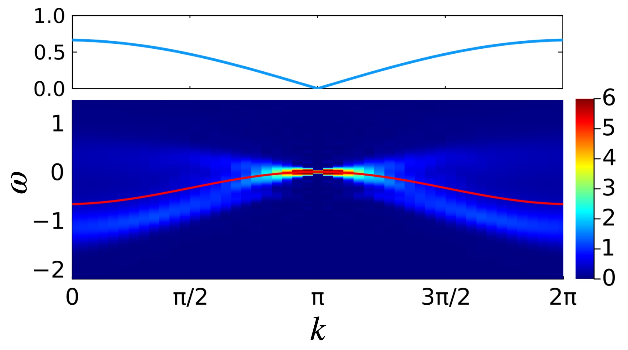
Figure 4: Bottom: Spectral function $A(k,\omega)$ of the original AKLT mode, and energy expectation $\varepsilon_{k}$. Top: energy variance $\delta\varepsilon_{k}$.

In practice, we usually focus on the translational-invariant Hamiltonian. That is, the trial operator will be in the form:

$$\hat{O}^{(i)}=\sum_{j=1}^{N}\hat{o}^{(i)}_{j}$$ (84)

For spin-1 degree of freedom, we first choose the basis for the local operators. A canonical choice is the Gell-Mann matrices:

$$\lambda^{(1)} =\left(\begin{array}[]{ccc}0&1&0\\ 1&0&0\\ 0&0&0\\ \end{array}\right), \lambda^{(2)} =\left(\begin{array}[]{ccc}0&-i&0\\ i&0&0\\ 0&0&0\\ \end{array}\right),$$ (85)

$$\lambda^{(3)} =\left(\begin{array}[]{ccc}1&0&0\\ 0&-1&0\\ 0&0&0\\ \end{array}\right), \lambda^{(4)} =\left(\begin{array}[]{ccc}0&0&1\\ 0&0&0\\ 1&0&0\\ \end{array}\right),$$

$$\lambda^{(5)} =\left(\begin{array}[]{ccc}0&0&-i\\ 0&0&0\\ i&0&0\\ \end{array}\right), \lambda^{(6)} =\left(\begin{array}[]{ccc}0&0&0\\ 0&0&1\\ 0&1&0\\ \end{array}\right),$$

$$\lambda^{(7)} =\left(\begin{array}[]{ccc}0&0&0\\ 0&0&-i\\ 0&i&0\\ \end{array}\right), \lambda^{(8)} =\frac{1}{\sqrt{3}}\left(\begin{array}[]{ccc}1&0&0\\ 0&1&0\\ 0&0&-2\\ \end{array}\right).$$

For two-site operators, we define

$$\hat{\lambda}^{(i,j)}\equiv\hat{\lambda}^{(i)}\otimes\hat{\lambda}^{(j)},\quad\hat{\lambda}^{[i,j]}\equiv\hat{\lambda}^{(i,j)}-\hat{\lambda}^{(j,i)}.$$ (86)

To find perturbations that induce nonzero velocity, we need to consider the odd-parity operators. For simplicity, we only consider $S^{z}_{\text{tot}}$-conserving, translational-invariant Hamiltonian. There are 6 independent odd-parity two-site operators:

$$\hat{o}^{(1)} =\hat{\lambda}^{[38]},$$ (87)

$$\hat{o}^{(2)} =\hat{\lambda}^{[12]},$$

$$\hat{o}^{(3)} =\hat{\lambda}^{[45]},$$

$$\hat{o}^{(4)} =\hat{\lambda}^{[67]},$$

$$\hat{o}^{(5)} =\hat{\lambda}^{[16]}+\hat{\lambda}^{[27]},$$

$$\hat{o}^{(6)} =\hat{\lambda}^{[17]}+\hat{\lambda}^{[62]}.$$

We do not find any solution for perturbation in the nearest-neighbor odd-parity operator space. However, we can further search for the three-site operator in the form:

$$\hat{\lambda}_{j}^{(a)}\hat{o}_{j-1,j+1}^{(b)},\quad a=3,8;\ b=1,\dots,6.$$

We find two independent solutions:

$$\hat{V}_{1} =\sum_{j=1}^{N}\left[\hat{\lambda}^{(3)}_{j}\otimes\hat{o}^{(2)}_{j-1,j+1}-\hat{s}^{z}_{j}\otimes\hat{o}^{(3)}_{j-1,j+1}+\hat{b}_{j}\otimes\hat{o}^{(4)}_{j-1,j+1}\right],$$

$$\hat{V}_{2} =\sum_{j=1}^{N}\hat{s}_{j}^{z}\otimes\left[\hat{o}^{(2)}+\hat{o}^{(4)}+2\hat{o}^{(6)}\right]_{j-1,j+1},$$

where we have defined the operator

$$\hat{b}=\frac{\sqrt{3}}{2}\hat{\lambda}^{(8)}-\frac{1}{2}\hat{\lambda}^{(3)}=\operatorname{diag}(0,1,-1).$$ (88)

D.2 Quasi-Nambu-Goldstone modes

The generalized scar Hamiltonian for AKLT tower is

$$\hat{H}(\alpha,\beta)=\hat{H}_{\text{AKLT}}+\alpha\hat{V}_{1}+\beta\hat{V}_{2},$$ (89)

where the (degenerate) AKLT model is fixed to

$$\hat{H}_{\text{AKLT}}=\sum_{j}\left[\frac{1}{2}\hat{\mathbf{s}}_{j}\cdot\hat{\mathbf{s}}_{j+1}+\frac{1}{6}(\hat{\mathbf{s}}_{j}\cdot\hat{\mathbf{s}}_{j+1})^{2}-\hat{s}^{z}_{j}\right],$$

and $\alpha,\beta$ are two free parameters. In the main text, the parameters are fixed to:

$$\hat{V}=-0.3\hat{V}_{1}-0.1\hat{V}_{2}.$$ (90)

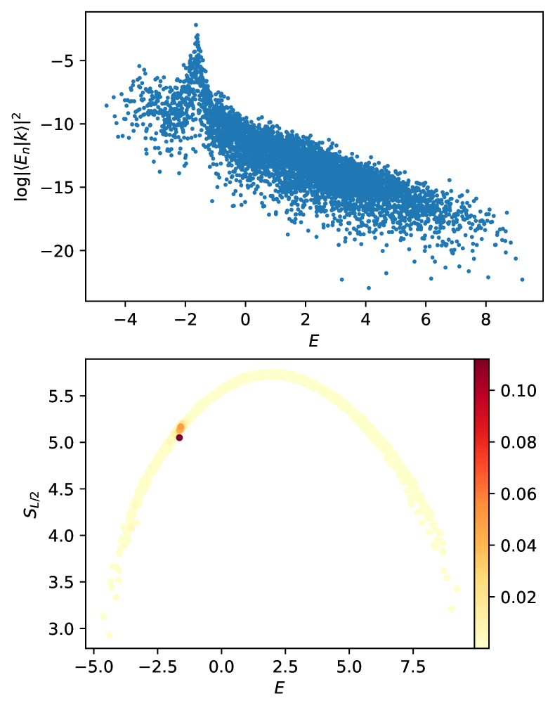
Figure 5: Exact diagonalization of Eq. (89) for a finite system with $L=12$ in the $(N=8,k=\pi+2\pi/L)$ sector. Top: Overlap between the initial state and each eigenstate. Bottom: Scatter plot of eigenenergy versus energy, with a color map indicating the overlaps with the z-quasi-Goldstone mode..

In Fig. 5, we show explicitly that Eq. (89) in the

$$k=\pi+\frac{2\pi}{L}$$

sector is indeed thermal and the z-quasi-Goldstone mode is the superposition of those thermal states.

Appendix E Deformed Quasi-Nambu-Goldstone Modes in Other Scar Models

In this Appendix, we delve deeper into examples showcasing deformed quasi-Goldstone modes within existing exact scar models. Specifically, we explore the Rydberg-antiblockaded scar model, the Onsager scar model, and an additional scar in the spin-1 XY model. Note that the original Hamiltonians of these scar models exhibit reflection symmetry, resulting in zero velocity at $k=0$ or $k=\pi$. To yield more nontrivial results, we introduce a deformation term $\hat{V}$ to the Hamiltonian:

$$\hat{H}^{\prime}=\hat{H}+\hat{V},$$ (91)

where $\hat{V}$ is reflection anti-symmetric, preserves the scar space, and induces nonzero velocity at the $k=0,\pi$.

E.1 Rydberg-antiblockaded model

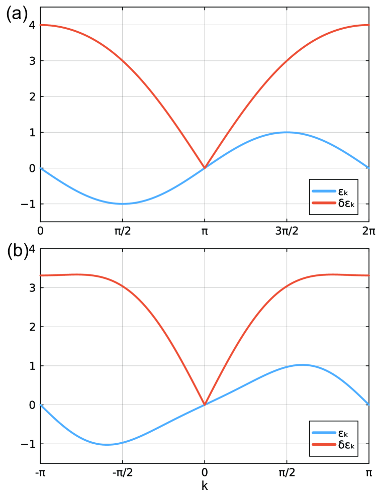
Figure 6: Energy expectation $\varepsilon_{k}$ and variance $\delta\varepsilon_{k}$ under deformed scar Hamiltonian Eq. (96) with $J=1,h=0,g=2$. (a) $\varepsilon_{k}$ and and $\delta\varepsilon_{k}$ of the z-qNGM in Eq. (95). (b) $\varepsilon_{k}$ and $\delta\varepsilon_{k}$ of the x-qNGM in Eq. (100) with $\xi=1/2$.

The model is introduced in Ref. Yang et al. (2020); Iadecola and Schecter (2020), with the Hamiltonian:

$$\hat{H}_{\text{Ryd}}=\sum_{j}\left[2J(\hat{s}_{j}^{x}-4\hat{s}_{j-1}^{z}\hat{s}_{j}^{x}\hat{s}_{j+1}^{z})+h\hat{s}_{j}^{z}\right]$$ (92)

It was proved that there is an exact scar tower, starting from the spin-all-down state $|\Psi_{0}\rangle=\left|\downarrow\cdots\downarrow\right\rangle$, and generated by the ladder:

$$\hat{Q}^{+} =\sum_{j}(-1)^{j}\hat{P}_{j-1}^{\downarrow}\hat{s}_{j}^{+}\hat{P}_{j+1}^{\downarrow},$$ (93)

$$|\Psi_{n}\rangle =(\hat{Q}^{+})^{n}|\Psi_{e}\rangle.$$

In Ref. Ren et al. (2022), the scar tower $\{|\Psi_{n}\rangle\}$ can be regarded as a deformed SU(2)-symmetric space deformed by an MPO with tensor:

$$W=\begin{bmatrix}0&\hat{s}^{+}\\ \hat{s}^{-}&\hat{P}^{\downarrow}\end{bmatrix}.$$ (94)

Since the scar tower has a ladder operator, the z-qNGM is simply defined as:

$$|k,z\rangle =\hat{W}\left[\hat{S}_{k}^{+}\left(\includegraphics[width=30.35657pt,valign={c}]{pics/spin-down}\otimes\cdots\otimes\includegraphics[width=30.35657pt,valign={c}]{pics/spin-down}\right)\right]$$ (95)

$$=\sum_{j}e^{ikj}\hat{P}_{j-1}^{\downarrow}\hat{s}_{j}^{+}\hat{P}_{j+1}^{\downarrow}|\Psi_{0}\rangle$$

$$=\sum_{j}e^{ikj}\hat{s}_{j}^{+}|\Psi_{0}\rangle.$$

We consider the deformed Hamiltonian:

$$\hat{H} =\hat{H}_{\text{Ryd}}+g\hat{V},$$ (96)

$$\hat{V} =\sum_{j}\left(\hat{s}_{j-1}^{x}\hat{s}_{j}^{y}\hat{s}_{j+1}^{z}-\hat{s}_{j-1}^{z}\hat{s}_{j}^{y}\hat{s}_{j+1}^{x}\right).$$

Fig. 6(a) shows the energy expectation and variance of the z-qNGM.

For the scar initial state being the following matrix-product state:

$$|\psi_{\xi}\rangle =\hat{W}\left[\includegraphics[width=30.35657pt,valign={c}]{pics/spin_theta}\otimes\includegraphics[width=30.35657pt,valign={c}]{pics/spin_mtheta}\otimes\cdots\right]$$ (97)

$$=|[ABAB\cdots AB]\rangle.$$

Here the tensors $A,B$ are:

$$A =W\cdot(\left|\downarrow\right\rangle+\xi\left|\uparrow\right\rangle)=\begin{bmatrix}0&\left|\uparrow\right\rangle\\ \xi\left|\downarrow\right\rangle&\left|\downarrow\right\rangle\end{bmatrix},$$ (98)

$$B =W\cdot(\left|\downarrow\right\rangle-\xi\left|\uparrow\right\rangle)=\begin{bmatrix}0&\left|\uparrow\right\rangle\\ -\xi\left|\downarrow\right\rangle&\left|\downarrow\right\rangle\end{bmatrix}.$$

where $\xi$ is related to the angle $\theta$:

$$\xi=\tan(\theta/2)$$ (99)

The energy expectation of the x-qNGM depends on $\xi$, in this specific model, when choosing $\xi=1$, the velocity at $k=0$ is zero. For this reason we instead choose $\xi=1/2$ so that the x-qNGM has nonzero velocity.

The x-qNGM is then defined as:

$$|k,x\rangle=\hat{S}_{k}^{z}|\psi_{\xi}\rangle=\sum_{j}e^{ikj}\hat{s}^{+}_{j}|\psi_{\xi}\rangle.$$ (100)

In Fig. 6(b), we display the energy expectation and variance of the x-qNGM.

E.2 Spin-1/2 Onsager scar model

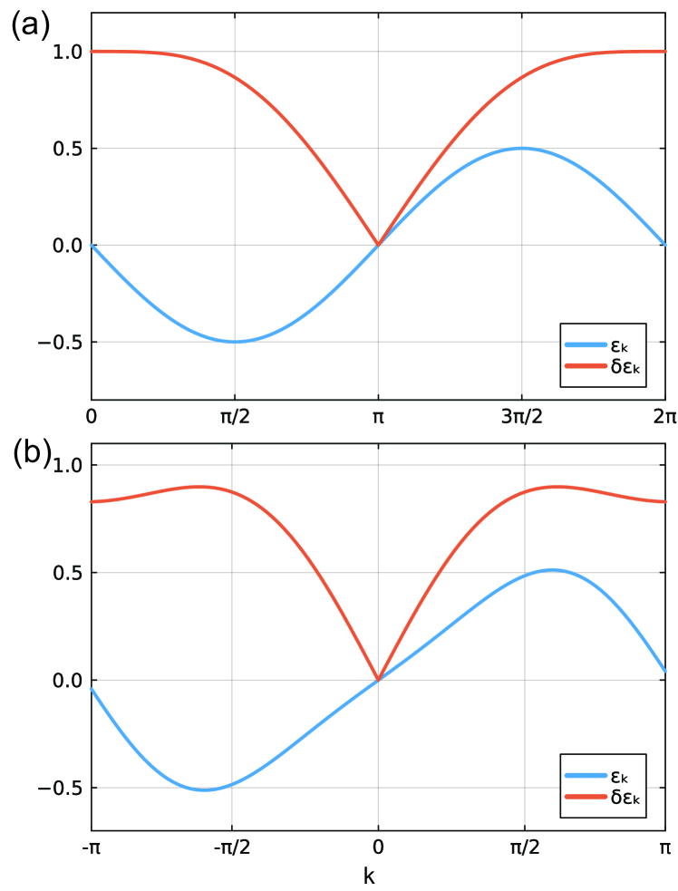
Figure 7: Energy expectation $\varepsilon_{k}$ and variance $\delta\varepsilon_{k}$ under Hamiltonian Eq. (101) with $n=2,h=0,\lambda=1/2$. (a) $\varepsilon_{k}$ and and $\delta\varepsilon_{k}$ of the z-qNGM in Eq. (107). (b) $\varepsilon_{k}$ and $\delta\varepsilon_{k}$ of the x-qNGM in Eq. (110) with $\xi=1/2$.

In Ref. Shibata et al. (2020), the following scar Hamiltonian was proposed

$$\hat{H}_{\text{Ons}}=\hat{H}_{n}+\lambda\hat{H}_{\text{pert}}+h\hat{S}^{z}.$$ (101)

Here, $\hat{H}_{n}$ is defined as

$$\hat{H}_{n}= \ -\sum_{j=1}^{L}\sum_{a=1}^{n-1}\frac{1}{4\sin(\pi a/n)}\left[n(-1)^{a}\left(\hat{s}_{j}^{-}\hat{s}_{j+1}^{+}\right)^{a}+\text{H.c.}\right.$$ (102)

$$\left.+(n-2a)\omega^{a/2}\hat{\tau}_{j}^{a}\right],$$

where $\omega=\exp(2\pi i/n)$, and the operator $\hat{\tau}=\operatorname{diag}(1,\omega,\dots,\omega^{n-1})$. We only consider the simplest $n=2$ case, where $\hat{H}_{n}$ is reduced to the spin-1/2 XY model:

$$\hat{H}_{2}=\sum_{j=1}^{L}\hat{s}_{j}^{x}\hat{s}_{j+1}^{x}+\hat{s}_{j}^{y}\hat{s}_{j+1}^{y}.$$ (103)

For the $n=2$ case, the ladder operator

$$\hat{Q}^{+}=\sum_{j}(-1)^{j}\hat{s}_{j}^{+}\hat{s}_{j+1}^{+}.$$ (104)

In Ref. Ren et al. (2022), this scar tower has been regarded as the deformed-SU(2) symmetric space. The MPO tensor of the deforming operator is:

$$W=\begin{bmatrix}\left|\downarrow\right\rangle\left\langle\downarrow\right|&\left|\uparrow\right\rangle\left\langle\downarrow\right|\\ \left|\uparrow\right\rangle\left\langle\uparrow\right|&0\end{bmatrix}$$ (105)

Also, here we choose the $\hat{H}_{\text{pert}}$ as

$$\hat{H}_{\text{pert}}=\sum_{j}\left(\hat{s}_{j-1}^{x}\hat{s}_{j+1}^{y}-\hat{s}_{j-1}^{y}\hat{s}_{j+1}^{x}\right).$$ (106)

The z-qNGM is

$$|k,z\rangle =\hat{W}\left[\hat{S}_{k}^{+}\left(\includegraphics[width=30.35657pt,valign={c}]{pics/spin-down}\otimes\cdots\otimes\includegraphics[width=30.35657pt,valign={c}]{pics/spin-down}\right)\right]$$ (107)

$$=\hat{Q}^{+}_{k}|\Psi_{0}\rangle$$

$$=\sum_{j}e^{ikj}\hat{s}_{j}^{+}\hat{s}_{j+1}^{+}|\Psi_{0}\rangle.$$

In Fig. 7(a), we show the energy expectation and variance of the z-qNGM.

For scar initial state being the matrix-product state

$$|\psi_{\xi}\rangle =\hat{W}\left[\includegraphics[width=30.35657pt,valign={c}]{pics/spin_theta}\otimes\includegraphics[width=30.35657pt,valign={c}]{pics/spin_mtheta}\otimes\cdots\right]$$ (108)

$$=|[ABAB\cdots AB]\rangle,$$

where the tensors $A,B$ are:

$$A =W\cdot(\left|\downarrow\right\rangle+\xi\left|\uparrow\right\rangle)=\begin{bmatrix}\left|\downarrow\right\rangle&\left|\uparrow\right\rangle\\ \xi\left|\uparrow\right\rangle&0\end{bmatrix},$$ (109)

$$B =W\cdot(\left|\downarrow\right\rangle-\xi\left|\uparrow\right\rangle)=\begin{bmatrix}\left|\downarrow\right\rangle&\left|\uparrow\right\rangle\\ -\xi\left|\uparrow\right\rangle&0\end{bmatrix}.$$

The x-qNGM is then defined as:

$$|k,x\rangle=\hat{S}_{k}^{z}|\psi_{\xi}\rangle=\sum_{j}e^{ikj}\hat{s}^{z}_{j}|\psi_{\xi}\rangle.$$ (110)

In Fig. 7(b), we display the energy expectation and variance of the x-qNGM.

E.3 Type-II scar tower in spin-1 XY model

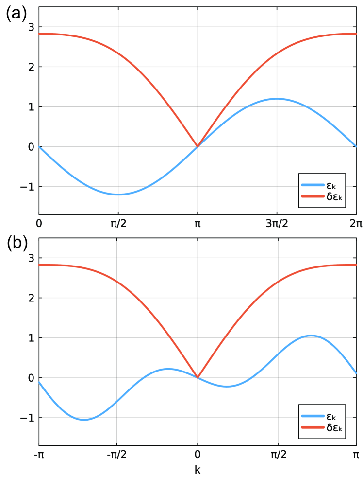
Figure 8: Energy expectation $\varepsilon_{k}$ and variance $\delta\varepsilon_{k}$ under Hamiltonian Eq. (118) with $h=0,\epsilon=0.1,\lambda=0.3$. (a) $\varepsilon_{k}$ and and $\delta\varepsilon_{k}$ of the z-qNGM in Eq. (114). (b) $\varepsilon_{k}$ and $\delta\varepsilon_{k}$ of the x-qNGM in Eq. (115).

In Ref. Schecter and Iadecola (2019), it was discovered that in spin-1 XY model, besides the original scar tower, another special scar tower emerges when the Hamiltonian is given by:

$$\hat{H}_{\text{XY}}= \ \sum_{j}\left[\hat{s}_{j}^{x}\hat{s}_{j+1}^{x}+\hat{s}_{j}^{y}\hat{s}_{j+1}^{y}+h\hat{s}_{j}^{z}\right.$$ (111)

$$\left.+\epsilon(\hat{s}_{j}^{+})^{2}(\hat{s}_{j+1}^{-})^{2}+\epsilon(\hat{s}_{j}^{-})^{2}(\hat{s}_{j+1}^{+})^{2}\right].$$

This additional scar tower originates from $|\Psi_{0}\rangle=|-\cdots-\rangle$, and is expressed as:

$$\left|\Psi_{n}\right\rangle\propto\sum_{i_{1}\neq i_{2}\neq\cdots\neq i_{n}}(-1)^{\sum_{j=1}^{n}i_{j}}\bigotimes_{j=1}^{n}\left(\hat{s}_{i_{j}}^{+}\hat{s}_{i_{j}+1}^{+}\right)\left|\Psi_{0}\right\rangle.$$ (112)

It is important to note that this scar tower lacks a local ladder operator. In Ref. Chattopadhyay et al. (2020), and later in Ref. Ren et al. (2022), this tower was interpreted as a projected SU(2)-symmetric space. The projector can be represented by an MPO, described by the tensor:

$$W=\begin{bmatrix}|+\rangle\left\langle\uparrow\right|&|0\rangle\left\langle\downarrow\right|\\ |0\rangle\left\langle\uparrow\right|&|-\rangle\left\langle\downarrow\right|\end{bmatrix}.$$ (113)

For the z-qNGM, it is defined as:

$$|k,z\rangle =\hat{W}\left[\hat{S}_{k}^{+}\left(\includegraphics[width=30.35657pt,valign={c}]{pics/spin-down}\otimes\cdots\otimes\includegraphics[width=30.35657pt,valign={c}]{pics/spin-down}\right)\right]$$ (114)

$$=\sum_{j}e^{ikj}\hat{s}_{j}^{+}\hat{s}_{j+1}^{+}|\Psi_{0}\rangle.$$

For the x-qNGM, the definition is similar as before:

$$|\psi_{\xi=1}\rangle =\hat{W}\left[\includegraphics[width=30.35657pt,valign={c}]{pics/spin-front}\otimes\includegraphics[width=30.35657pt,valign={c}]{pics/spin-back}\otimes\cdots\right]$$ (115)

$$=|[ABAB\cdots AB]\rangle,$$

where $|\Psi_{\xi}\rangle=|[AB\cdots AB]\rangle$ has the MPS representation:

$$A =W\cdot(\left|\downarrow\right\rangle+\xi\left|\uparrow\right\rangle)=\begin{bmatrix}|+\rangle&|0\rangle\\ |0\rangle&|-\rangle\end{bmatrix},$$ (116)

$$B =W\cdot(\left|\downarrow\right\rangle-\xi\left|\uparrow\right\rangle)=\begin{bmatrix}-|+\rangle&|0\rangle\\ -|0\rangle&|-\rangle\end{bmatrix}.$$

The energy expectation and variance are displayed in Fig. 8. For this additional tower, we introduce the deformation:

$$\hat{H}=\hat{H}_{\text{XY}}+\lambda\hat{V},$$ (117)

where the perturbation term is defined as:

$$\hat{V}= \ \sum_{j}\left[\hat{\lambda}^{(3)}_{j}\otimes\hat{\lambda}^{[1,2]}_{j-1,j+1}+\hat{b}_{j}\otimes\hat{\lambda}^{[6,7]}_{j-1,j+1}\right.$$ (118)

$$+\left.\hat{s}^{z}_{j}\otimes\left(\hat{\lambda}^{[1,7]}_{j-1,j+1}-\hat{\lambda}^{[2,6]}_{j-1,j+1}\right)\right]$$

using the notation in Eq. (86).

Appendix F Quasi-Nambu-Goldstone Modes in SU(3) Scar Model

Now we consider the scar tower with SU(3) quasisymmetry, constructed in Ref. Ren et al. (2021). This is a spin-1 chain hosting a maximal weight representation of SU(3).

F.1 SU(3) scar model

In the SU(3) scar model, the anchor state is fixed to the polarized state $|\Psi_{e}\rangle=\left|-\cdots-\right\rangle$. The SU(3)-symmetric space, according to the definition, is

$$\mathcal{H}_{\mathrm{SU(3)}}\equiv\operatorname{span}\{\hat{u}(g)^{\otimes N}|\Psi_{e}\rangle|\forall g\in\mathrm{SU(3)}\}.$$ (119)

From the representation theory of Lie algebra, the space $\mathcal{H}_{\mathrm{SU(3)}}$ is the maximal weight irreducible representation. An orthonormal basis for $\mathcal{H}_{\mathrm{SU(3)}}$ can be generated by acting the following ladder operator

$$\hat{Q}_{1}^{+} =\sum_{j}(\hat{q}_{1}^{+})_{j}=\begin{pmatrix}0&&\\ &0&1\\ &&0\end{pmatrix}_{j},$$ (120)

$$\hat{Q}_{2}^{+} =\sum_{j}(\hat{q}_{2}^{+})_{j}=\sum_{j}\begin{pmatrix}0&&1\\ &0&\\ &&0\end{pmatrix}_{j}.$$

to the anchor state $|\Psi_{e}\rangle$. That is,

$$\mathcal{H}_{\mathrm{SU(3)}}=\operatorname{span}\{(\hat{Q}_{1}^{+})^{n}(\hat{Q}_{2}^{+})^{m}|\Psi_{e}\rangle|\forall n,m\in\mathrm{SU(3)}\}.$$ (121)

With the scar space defined, we can use the quantum inverse method to find all the possible translational invariant nearest-neighbor scar Hamiltonians.

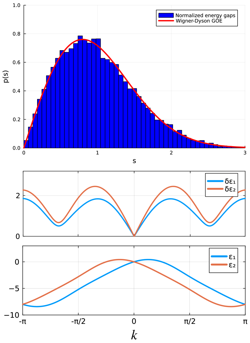
Figure 9: Top: Spectrum of the $L=12$ SU(3)-scar model with Hilber space dimension $\dim\mathcal{H}=52488$. The model parameters are fixed to be $J_{1}=1,\ J_{2}=-0.6,\ J_{3}=0.3,\ J_{4}=0.2,\ J_{5}=0.1,\ J_{6}=0.3$. Statistics of energy gaps in the middle half of the ($k=0$) sector show the Wigner-Dyson GOE form, indicating non-integrability. Middle: energy variance of two modes in SU(3) scar model. Bottom: energy expectation of two modes.

There are in total 9 solutions from the quantum inverse method:

$$\hat{o}^{(1)}_{j,j+1} =\sum_{a=1}^{8}\hat{\lambda}_{j,j+1}^{(aa)},$$

$$\hat{o}^{(2)}_{j,j+1} =\hat{\lambda}_{j,j+1}^{[12]}+\hat{\lambda}_{j,j+1}^{[45]},$$

$$\hat{o}^{(3)}_{j,j+1} =\hat{\lambda}_{j,j+1}^{[45]}+\hat{\lambda}_{j,j+1}^{[67]},$$

$$\hat{o}^{(4)}_{j,j+1} =2\hat{\lambda}_{j,j+1}^{[13]}-\hat{\lambda}_{j,j+1}^{[46]}-\hat{\lambda}_{j,j+1}^{[57]},$$

$$\hat{o}^{(5)}_{j,j+1} =2\hat{\lambda}_{j,j+1}^{[23]}+\hat{\lambda}_{j,j+1}^{[47]}-\hat{\lambda}_{j,j+1}^{[56]},$$

$$\hat{o}^{(6)}_{j,j+1} =\hat{\lambda}_{j,j+1}^{[14]}+\hat{\lambda}_{j,j+1}^{[25]}-\hat{\lambda}_{j,j+1}^{[36]}-\sqrt{3}\hat{\lambda}_{j,j+1}^{[48]},$$

$$\hat{o}^{(7)}_{j,j+1} =\hat{\lambda}_{j,j+1}^{[15]}-\hat{\lambda}_{j,j+1}^{[24]}-\hat{\lambda}_{j,j+1}^{[37]}-\sqrt{3}\hat{\lambda}_{j,j+1}^{[78]},$$

$$\hat{o}^{(8)}_{j,j+1} =\hat{\lambda}_{j,j+1}^{[16]}-\hat{\lambda}_{j,j+1}^{[27]}+\hat{\lambda}_{j,j+1}^{[34]}-\sqrt{3}\hat{\lambda}_{j,j+1}^{[48]},$$

$$\hat{o}^{(9)}_{j,j+1} =\hat{\lambda}_{j,j+1}^{[17]}+\hat{\lambda}_{j,j+1}^{[26]}+\hat{\lambda}_{j,j+1}^{[35]}-\sqrt{3}\hat{\lambda}_{j,j+1}^{[58]}.$$

Note that one of them is Heisenberg-like (SU(3) singlet), and 8 are DM-like (SU(3)-octet). Besides, these interactions are not limited to nearest neighbor. That is, $\sum_{j}\hat{o}_{j,j+d}^{(n)}$ for any $d\geq 1$ is a parent Hamiltonian for the scar tower. Choose the Hamiltonian form:

$$\hat{H}= \ \sum_{j}\left(J_{1}\hat{o}^{(1)}_{j,j+1}+J_{2}\hat{o}^{(2)}_{j,j+1}+J_{3}\hat{o}^{(3)}_{j,j+1}\right.$$ (122)

$$\left.+J_{4}\hat{o}^{(4)}_{j,j+2}+J_{5}\hat{o}^{(6)}_{j,j+2}+J_{6}\hat{o}^{(6)}_{j,j+3}\right),$$

where the local terms of $\hat{O}^{(4)}$ and $\hat{O}^{(6)}$ act on next-nearest neighbor sites. We choose

$$J_{1} =1,\quad J_{2}=-0.6,\quad J_{3}=0.3,$$ (123)

$$J_{4} =0.2,\quad J_{5}=0.1,\quad J_{6}=0.3.$$

The finite-size exact diagonalization shows clear Wigner-Dyson level statistics, see Fig. 9a.

F.2 Multiple quasi-Nambu-Goldstone modes

The nature definitions of quasi-Goldstone modes in this case are

$$|k,1\rangle =\sum_{j}e^{ikj}(\hat{q}_{1}^{+})_{j}|\Psi_{e}\rangle,$$ (124)

$$|k,2\rangle =\sum_{j}e^{ikj}(\hat{q}_{2}^{+})_{j}|\Psi_{e}\rangle.$$

Note that the transition amplitude for the two modes are

$$\langle k,a|H|k,b\rangle=\begin{bmatrix}\varepsilon_{1}&v\\ v^{*}&\varepsilon_{2}\end{bmatrix}_{ab},$$ (125)

where

$$\varepsilon_{1} =4J_{1}[\cos(k)-1]-4J_{3}\sin(k),$$

$$\varepsilon_{2} =4J_{1}[\cos(k)-1]-4\left(J_{2}+J_{3}\right)\sin(k),$$

$$v =4i\sin(2k)J_{4}.$$

Because of the transition amplitude, we choose to define the qNGMs as the linear combinations of the $|k,1\rangle$ and $|k,2\rangle$, so that the two modes are decoupled, with energy expectation:

$$\varepsilon_{\pm}(k)= \ 4J_{1}[\cos(k)-1]-\left(2J_{2}+4J_{3}\right)\sin(k)$$ (126)

$$\pm 2\sin(k)\sqrt{J_{2}^{2}+16J_{4}^{2}\cos^{2}(k)}$$

$$= \ -2\left[J_{2}+2J_{3}\pm\sqrt{J_{2}^{2}+16J_{4}^{2}}\right]k+O\left(k^{2}\right).$$

Because of the linear combination, the exact expression of the energy variance for the mode becomes complicated. In Fig. 9b, we plot the energy expectation and energy variance for each independent mode.

Appendix G Quasi-Nambu-Goldstone Modes in Deformed PXP Model

In this section, we explore the PXP model pxp-1; pxp-2:

$$\hat{H}=\sum_{j}\hat{P}^{\downarrow}_{j-1}\hat{\sigma}_{j}^{x}\hat{P}^{\downarrow}_{j-1},$$ (127)

which serves as the effective model for the Rydberg atom array experiment Bernien et al. (2017). This model is notable for featuring an approximate scar tower without an exact symmetry structure. Despite the absence of precise symmetry, the PXP model exhibits an approximate decoupling

$$\hat{H}_{\text{PXP}}\approx\hat{H}_{\text{FSA}}\oplus\hat{H}_{\text{th}},$$ (128)

where a special subspace is generated by the forward scattering approximation (FSA) pxp-1.

In the FSA, the Hamiltonian $\hat{H}$ Eq. (127) is decomposed into $\hat{H}=\hat{H}^{+}+\hat{H}^{-}$, where

$$\hat{H}^{-} =\sum_{j\in\text{odd}}\hat{P}^{\downarrow}_{j-1}\hat{\sigma}_{j}^{+}\hat{P}^{\downarrow}_{j-1}+\sum_{j\in\text{even}}\hat{P}^{\downarrow}_{j-1}\hat{\sigma}_{j}^{-}\hat{P}^{\downarrow}_{j-1},$$

$$\hat{H}^{+} =\sum_{j\in\text{odd}}\hat{P}^{\downarrow}_{j-1}\hat{\sigma}_{j}^{-}\hat{P}^{\downarrow}_{j-1}+\sum_{j\in\text{even}}\hat{P}^{\downarrow}_{j-1}\hat{\sigma}_{j}^{+}\hat{P}^{\downarrow}_{j-1}.$$

Within this approximation, the quasi-periodic dynamics originating from the initial Neel state

$$|\mathbb{Z}_{2}\rangle\equiv\left|\uparrow\downarrow\cdots\uparrow\downarrow\right\rangle.$$

is primarily contained within the FSA subspace:

$$\mathcal{H}_{\text{FSA}}=\operatorname{span}\left\{\left.(\hat{H}^{+})^{n}|\mathbb{Z}_{2}\rangle\right|\forall n\in\mathbb{Z}^{+}\right\}.$$ (129)

This subspace is spanned by states generated through the application of $\hat{H}^{+}$ on the initial $|\mathbb{Z}_{2}\rangle$ state, eventually reaching another Neel state:

$$|\mathbb{Z}_{2}^{\prime}\rangle=\left|\downarrow\uparrow\cdots\downarrow\uparrow\right\rangle.$$

G.1 Approximate SU(2) and the corresponding quasi-Nambu-Goldstone modes

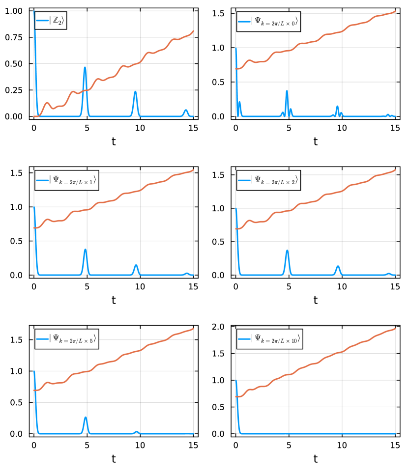
Figure 10: Scar dynamics (for system size $L=50$) initiated from $|\mathbb{Z}_{2}\rangle$ and $|\Psi_{k=2\pi n/L}\rangle$’s, where $n\in\{0,1,2,5,10\}$. The evolution is based on MPS TDVP simulation with bond dimension $\chi=60$. The blue lines represent the evolution of fidelity $F(t)=|\langle\psi|\psi(t)\rangle|^{2}$, and the orange line represents the evolution of the bipartite entanglement entropy.

The operators $\hat{H}^{+}$ and $\hat{H}^{-}$, along with their commutator $[\hat{H}^{+},\hat{H}^{-}]$, form an approximate SU(2) algebra:

$$\hat{H}^{\pm}=\frac{\Delta}{2}\hat{S}^{\pm},\quad\hat{S}^{z}=\frac{1}{2}[\hat{S}^{+},\hat{S}^{-}]=\frac{1}{\Delta}[\hat{H}^{+},\hat{H}^{-}].$$ (130)

In this context, the scar initial state $|\mathbb{Z}_{2}\rangle$ acts as the “bottom state” in the $s=L/2$ representation of this approximate SU(2) symmetry, which is evidenced by the relation $\hat{H}^{-}|\mathbb{Z}_{2}\rangle=0$. Within this subspace, the Hamiltonian simplifies:

$$\hat{H}=\hat{H}^{+}+\hat{H}^{-}\simeq\Delta\hat{S}^{x},$$ (131)

indicating scar dynamics akin to the rotation of a large spin with a period $T=2\pi/\Delta$. This approximate symmetry allows for other scar states, such as:

$$|\Psi_{0}\rangle\propto\hat{H}^{+}|\mathbb{Z}_{2}\rangle,$$ (132)

which also evolves approximately within the SU(2) subspace. The approximate. The approximate qNGM state is similarly defined by introducing small spatial modulation:

$$|\Psi_{k}\rangle= \ \sum_{j\in\text{odd}}e^{ikj}\hat{P}^{\downarrow}_{j-1}\hat{\sigma}_{j}^{-}\hat{P}^{\downarrow}_{j-1}|\mathbb{Z}_{2}\rangle$$ (133)

$$+\sum_{j\in\text{even}}e^{ikj}\hat{P}^{\downarrow}_{j-1}\hat{\sigma}_{j}^{+}\hat{P}^{\downarrow}_{j-1}|\mathbb{Z}_{2}\rangle.$$

For $|\mathbb{Z}_{2}\rangle$ state, the above expression has a simple form:

$$|\Psi_{k}\rangle\propto\sum_{j\in\text{odd}}e^{ikj}\hat{\sigma}_{j}^{-}|\mathbb{Z}_{2}\rangle.$$

A unique aspect of the PXP model is that there is no tuning parameter for the spacing of scar eigenstates, precluding the possibility of a degenerate limit. Consequently, the lifetime of the qNGM cannot be quantified by energy variance. Instead, we can demonstrate the long lifetime by directly simulating the evolution of the many-body fidelity and the growth of entanglement entropy.

To investigate the scar dynamics, we conducted numerical simulations starting from $|\Psi_{k}\rangle$ in a system of size $L=50$, employing the time-dependent variational principle (TDVP) algorithm Haegeman et al. (2011, 2016). Fig. 10 illustrates the time evolution beginning from $|\mathbb{Z}2\rangle$ and $|\Psi{k=2\pi n/L}\rangle$. Notably, for $k=2\pi/L$, the fidelity exhibits nearly identical evolution to that of $k=0$, the latter being regarded as within the FSA subspace.

G.2 Deformed PXP model and its quasi-Nambu-Goldstone modes

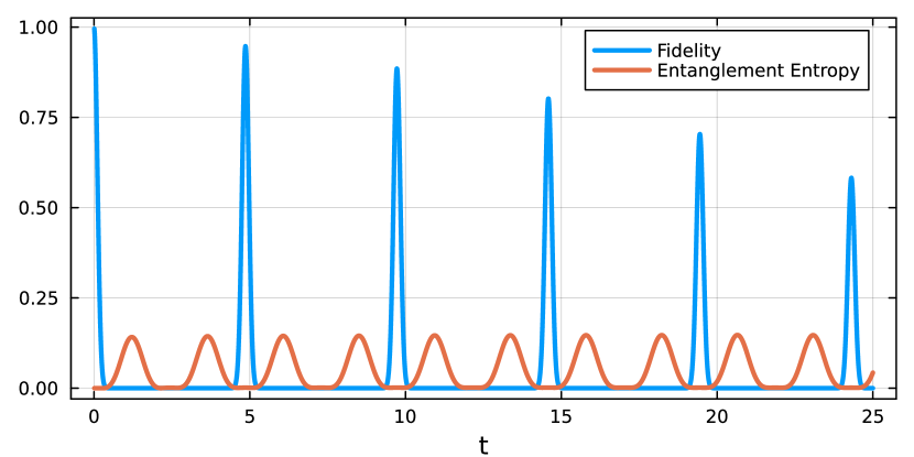
Figure 11: Dynamics of $|\mathbb{Z}_{2}\rangle$ under deformed PXP Hamiltonian Eq. (134). The system size is $L=100$, and the simulation is based on the MPS TDVP algorithm with maximum bond dimension $\chi=30$. The many-body fidelity shows quasi-periodic and the entanglement entropy remains small during the simulation time, which allows us to choose a small bond dimension.

Although the forward scattering approximation provides partial insight into the revival phenomena, it remains a coarse approximation for the PXP model. Moreover, the PXP scar dynamics exhibit a relatively short lifetime, complicating the quantification of the qNGM lifetime. To address this, we employ a deformed PXP model Choi et al. (2019), introducing modifications to the original Hamiltonian to enhance the SU(2) algebra in Eq. (130):

$$\hat{H}=\sum_{j}\hat{P}^{\downarrow}_{j-1}\hat{\sigma}_{j}^{x}\hat{P}^{\downarrow}_{j-1}\left[1-\sum_{d=2}^{R}h_{d}\left(\hat{\sigma}_{j-d}^{z}+\hat{\sigma}_{j+d}^{z}\right)\right].$$ (134)

For clarity, we introduce the following notation:

$$\hat{K}_{j}\equiv\hat{\mathbb{I}}-\sum_{d=2}^{R}h_{d}\left(\hat{\sigma}_{j-d}^{z}+\hat{\sigma}_{j+d}^{z}\right).$$ (135)

By setting:

$$h_{d}=\frac{h_{0}}{\left[\phi^{d-1}-\phi^{-(d-1)}\right]^{2}},$$ (136)

where $\phi=(\sqrt{5}+1)/2$ and $h_{0}$ is optimized numerically to approximately $0.051$ Choi et al. (2019), the decoupling in Eq. (128) is significantly improved, though remaining approximate. Subsequent analysis is based on this deformed PXP model with these specified parameters.

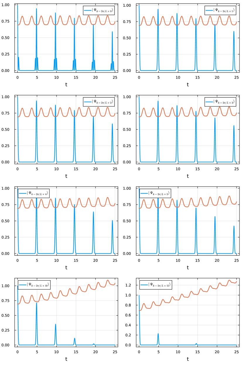
Figure 12: Scar dynamics initiated from $|\mathbb{Z}_{2}\rangle$ and $|\Psi_{k=2\pi n/L}\rangle$’s, where $n\in\{0,1,2,3,4,5,10,15\}$. The blue lines represent the evolution of fidelity $F(t)=|\langle\psi|\psi(t)\rangle|^{2}$, and the orange line represents the evolution of the bipartite entanglement entropy.

The deformed PXP model can also be expressed as $\hat{H}=\hat{H}^{-}+\hat{H}^{+}$, where

$$\hat{H}^{-} =\sum_{j\in\text{odd}}\hat{P}^{\downarrow}_{j-1}\hat{\sigma}_{j}^{+}\hat{P}^{\downarrow}_{j-1}\hat{K}_{j}+\sum_{j\in\text{even}}\hat{P}^{\downarrow}_{j-1}\hat{\sigma}_{j}^{-}\hat{P}^{\downarrow}_{j-1}\hat{K}_{j},$$

$$\hat{H}^{+} =\sum_{j\in\text{odd}}\hat{P}^{\downarrow}_{j-1}\hat{\sigma}_{j}^{-}\hat{P}^{\downarrow}_{j-1}\hat{K}_{j}+\sum_{j\in\text{even}}\hat{P}^{\downarrow}_{j-1}\hat{\sigma}_{j}^{+}\hat{P}^{\downarrow}_{j-1}\hat{K}_{j}.$$

With these parameters, in Eq.(130), we find $\Delta\approx 1.29$, resulting in a period $T\approx 4.86$. Fig. 11 presents a simulation of scar dynamics for a system of size $L=100$ starting from the $|\mathbb{Z}_{2}\rangle$ initial state. Notably, for $L=100$, any seemingly nonzero fidelity indicates that the state remains close to the original one. Another observation is the low entanglement entropy during the dynamics. In contrast to the original PXP model, as shown in the first panel of Fig. 10, where the entanglement entropy generally increases with minor dips, the deformed model shows prolonged periods of low entanglement entropy.

The qNGM is generated by the twisted ladder operator

$$\hat{H}^{+}_{k}=\sum_{j\in\text{odd}/\text{even}}e^{ikj}\hat{P}^{\downarrow}_{j-1}\hat{\sigma}_{j}^{-/+}\hat{P}^{\downarrow}_{j-1}\hat{K}_{j}.$$ (137)

The additional $\hat{K}_{j}$ term does not affect the $|\mathbb{Z}_{2}\rangle$ state. Therefore, the qNGM remains the same as in the original PXP model:

$$|\Psi_{k}\rangle=\hat{H}^{+}_{k}=\sum_{j\in\text{odd}}e^{ikj}\hat{\sigma}_{j}^{-}|\mathbb{Z}_{2}\rangle.$$

Refer to Fig. 12for the time evolution starting from $|\mathbb{Z}2\rangle$ and $|\Psi{k=2\pi n/L}\rangle$. Besides the quasi-oscillation of many-body fidelity, the bipartite entanglement entropy also displays approximate periodicity and remains low for extended durations.

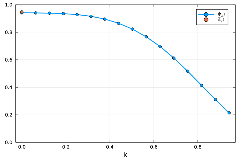
Figure 13: One-period fidelity $F(T)$ for initial state $|\mathbb{Z}_{2}\rangle$ as well as $|\Psi_{k}\rangle$’s. Note that $F_{k}(T)$ behaves like a continuous function of $k$.

Since the PXP model does not fall within the quasisymmetry framework and lacks a “degenerate limit,” we instead consider the evolution operator:

$$U(T)=\exp(-i\hat{H}_{\text{PXP}}T),\quad T\approx 4.86.$$ (138)

We interpret this operator as the Floquet operator, characterized by the following eigensystem:

$$U(T)|n\rangle=e^{-i\phi_{n}}|n\rangle.$$ (139)

For the initial state $|\psi(0)\rangle$, exhibiting nearly periodic time evolution, its Floquet spectral decomposition can be expressed as:

$$|\psi(0)\rangle\approx\sum_{\alpha}c_{\alpha}|\alpha\rangle,$$ (140)

where the dominant $c_{\alpha}$ coefficients correspond to nearly identical quasienergies $\phi_{\alpha}$. A natural approach to quantify the lifetime of the qNGM is to consider the one-period fidelity:

$$F_{k}(T)=|\langle\Psi_{k}|\Psi_{k}(T)\rangle|^{2}.$$ (141)

As shown in Fig. 13, $F_{k}(T)$ behaves as a continuous function of $k$; for small $k$, the fidelity decay closely resembles that of states in the subspace $\mathcal{H}_{\text{FSA}}$.

G.3 Spectrum

Figure 14: Exact diagonalization of a finite system with $L=28$ in the $(k=2\pi/L)+(k=\pi+2\pi/L)$ sector. (a) depicts the overlap between the initial state and each eigenstate. (b) illustrates the entanglement entropy of each eigenstate. (c) presents a scatter plot of eigenenergy versus energy, with a color map indicating the overlaps with the qNGMs defined in Eq. (133).

We examine the qNGM with the smallest nonzero momentum $k=\frac{2\pi}{L}$. Note that since the initial state is invariant only under a two-site shift, it spans both $k=\frac{2\pi}{L}$ and $k=\pi+\frac{2\pi}{L}$ sectors:

$$|\Psi_{k}\rangle=\frac{1}{\sqrt{2}}\left(|\Psi_{k}^{e}\rangle+|\Psi_{k}^{o}\rangle\right),$$ (142)

where $|k_{e}\rangle$ and $|k_{o}\rangle$ are projections of $|k\rangle$ onto each sector. Specifically:

$$|\Psi_{k}^{e}\rangle \propto\sum_{j\in\text{odd}}e^{ikj}\hat{\sigma}_{j}^{-}|\mathbb{Z}_{2}\rangle+\sum_{j\in\text{even}}e^{ikj}\hat{\sigma}_{j}^{-}|\mathbb{Z}_{2}^{\prime}\rangle,$$ (143)

$$|\Psi_{k}^{o}\rangle \propto\sum_{j\in\text{odd}}e^{ikj}\hat{\sigma}_{j}^{-}|\mathbb{Z}_{2}\rangle-\sum_{j\in\text{even}}e^{ikj}\hat{\sigma}_{j}^{-}|\mathbb{Z}_{2}^{\prime}\rangle,$$

where $|\mathbb{Z}_{2}^{\prime}\rangle$ serves as the “top state” in the approximate SU(2) representation.

Numerically, we perform exact diagonalization on a system of size $L=28$ to investigate the eigenstate overlap $|\langle E_{n}|k\rangle|^{2}$ and the bipartite entanglement entropy of each eigenstate. Specifically, we perform the diagonalization in the subspace:

$$\mathcal{H}=\mathcal{H}_{k=\frac{2\pi}{L}}\oplus\mathcal{H}_{k=\pi+\frac{2\pi}{L}}.$$ (144)

As depicted in Fig. 14(a), the eigenstate components exhibit strong overlaps with approximately equally-spaced eigenstates, suggesting nearly periodic evolution. However, as shown in Fig. 14(b), the subspace $\mathcal{H}$ lacks a set of low-entangled states, unlike the $(k=0)$ sector. Further illustrated in Fig. 14(c), although some states are relatively low-entangled, the majority exhibit high entanglement.

References

- Heisenberg (1928) W. Heisenberg, Zeitschrift für Physik 49, 619 (1928), URL https://doi.org/10.1007/BF01328601.
- Nambu and Jona-Lasinio (1961) Y. Nambu and G. Jona-Lasinio, Phys. Rev. 122, 345 (1961), URL https://link.aps.org/doi/10.1103/PhysRev.122.345.
- Goldstone et al. (1962) J. Goldstone, A. Salam, and S. Weinberg, Phys. Rev. 127, 965 (1962), URL https://link.aps.org/doi/10.1103/PhysRev.127.965.
- Nambu (2009) Y. Nambu, Rev. Mod. Phys. 81, 1015 (2009), URL https://link.aps.org/doi/10.1103/RevModPhys.81.1015.
- Bernien et al. (2017) H. Bernien, S. Schwartz, A. Keesling, H. Levine, A. Omran, H. Pichler, S. Choi, A. S. Zibrov, M. Endres, M. Greiner, et al., Nature 551, 579 (2017), URL https://doi.org/10.1038/nature24622.
- Affleck et al. (1987) I. Affleck, T. Kennedy, E. H. Lieb, and H. Tasaki, Phys. Rev. Lett. 59, 799 (1987), URL https://link.aps.org/doi/10.1103/PhysRevLett.59.799.
- Moudgalya et al. (2018a) S. Moudgalya, S. Rachel, B. A. Bernevig, and N. Regnault, Phys. Rev. B 98, 235155 (2018a), URL https://link.aps.org/doi/10.1103/PhysRevB.98.235155.
- Turner et al. (2018a) C. J. Turner, A. A. Michailidis, D. A. Abanin, M. Serbyn, and Z. Papić, Nat. Phys. 14, 745 (2018a), URL https://doi.org/10.1038/s41567-018-0137-5.
- Turner et al. (2018b) C. J. Turner, A. A. Michailidis, D. A. Abanin, M. Serbyn, and Z. Papić, Phys. Rev. B 98, 155134 (2018b), URL https://link.aps.org/doi/10.1103/PhysRevB.98.155134.
- Ho et al. (2019) W. W. Ho, S. Choi, H. Pichler, and M. D. Lukin, Phys. Rev. Lett. 122, 040603 (2019), URL https://doi.org/10.1103/PhysRevLett.122.040603.
- Choi et al. (2019) S. Choi, C. J. Turner, H. Pichler, W. W. Ho, A. A. Michailidis, Z. Papić, M. Serbyn, M. D. Lukin, and D. A. Abanin, Phys. Rev. Lett. 122, 220603 (2019), URL https://doi.org/10.1103/PhysRevLett.122.220603.
- Lin and Motrunich (2019) C.-J. Lin and O. I. Motrunich, Phys. Rev. Lett. 122, 173401 (2019), URL https://link.aps.org/doi/10.1103/PhysRevLett.122.173401.
- Bull et al. (2020) K. Bull, J.-Y. Desaules, and Z. Papić, Phys. Rev. B 101, 165139 (2020), URL https://link.aps.org/doi/10.1103/PhysRevB.101.165139.
- Khemani et al. (2019) V. Khemani, C. R. Laumann, and A. Chandran, Phys. Rev. B 99, 161101(R) (2019), URL https://link.aps.org/doi/10.1103/PhysRevB.99.161101.
- Michailidis et al. (2020) A. A. Michailidis, C. J. Turner, Z. Papić, D. A. Abanin, and M. Serbyn, Phys. Rev. X 10, 011055 (2020), URL https://link.aps.org/doi/10.1103/PhysRevX.10.011055.
- Turner et al. (2021) C. J. Turner, J.-Y. Desaules, K. Bull, and Z. Papić, Phys. Rev. X 11, 021021 (2021), URL https://link.aps.org/doi/10.1103/PhysRevX.11.021021.
- Iadecola et al. (2019) T. Iadecola, M. Schecter, and S. Xu, Phys. Rev. B 100, 184312 (2019), URL https://link.aps.org/doi/10.1103/PhysRevB.100.184312.
- Pan and Zhai (2022) L. Pan and H. Zhai, Phys. Rev. Res. 4, L032037 (2022), URL https://link.aps.org/doi/10.1103/PhysRevResearch.4.L032037.
- Moudgalya et al. (2018b) S. Moudgalya, N. Regnault, and B. A. Bernevig, Phys. Rev. B 98, 235156 (2018b), URL https://link.aps.org/doi/10.1103/PhysRevB.98.235156.
- Mark et al. (2020) D. K. Mark, C.-J. Lin, and O. I. Motrunich, Physical Rev. B 101, 195131 (2020), URL https://link.aps.org/doi/10.1103/PhysRevB.101.195131.
- Moudgalya et al. (2020a) S. Moudgalya, E. O’Brien, B. A. Bernevig, P. Fendley, and N. Regnault, Phys. Rev. B 102, 085120 (2020a), URL https://link.aps.org/doi/10.1103/PhysRevB.102.085120.
- Shiraishi (2019) N. Shiraishi, Journal of Statistical Mechanics: Theory and Experiment 2019, 083103 (2019), URL https://doi.org/10.1088%2F1742-5468%2Fab342e.
- Mark and Motrunich (2020) D. K. Mark and O. I. Motrunich, Phys. Rev. B 102, 075132 (2020), URL https://link.aps.org/doi/10.1103/PhysRevB.102.075132.
- Moudgalya et al. (2020b) S. Moudgalya, N. Regnault, and B. A. Bernevig, Phys. Rev. B 102, 085140 (2020b), URL https://link.aps.org/doi/10.1103/PhysRevB.102.085140.
- Schecter and Iadecola (2019) M. Schecter and T. Iadecola, Phys. Rev. Lett. 123, 147201 (2019), URL https://link.aps.org/doi/10.1103/PhysRevLett.123.147201.
- Chattopadhyay et al. (2020) S. Chattopadhyay, H. Pichler, M. D. Lukin, and W. W. Ho, Phys. Rev. B 101, 174308 (2020), URL https://link.aps.org/doi/10.1103/PhysRevB.101.174308.
- Shibata et al. (2020) N. Shibata, N. Yoshioka, and H. Katsura, Phys. Rev. Lett. 124, 180604 (2020), URL https://link.aps.org/doi/10.1103/PhysRevLett.124.180604.
- Yang et al. (2020) Z.-C. Yang, F. Liu, A. V. Gorshkov, and T. Iadecola, Phys. Rev. Lett. 124, 207602 (2020), URL https://link.aps.org/doi/10.1103/PhysRevLett.124.207602.
- Iadecola and Schecter (2020) T. Iadecola and M. Schecter, Phys. Rev. B 101, 024306 (2020), URL https://link.aps.org/doi/10.1103/PhysRevB.101.024306.
- Wildeboer et al. (2022) J. Wildeboer, C. M. Langlett, Z.-C. Yang, A. V. Gorshkov, T. Iadecola, and S. Xu, Phys. Rev. B 106, 205142 (2022), URL https://link.aps.org/doi/10.1103/PhysRevB.106.205142.
- Langlett et al. (2022) C. M. Langlett, Z.-C. Yang, J. Wildeboer, A. V. Gorshkov, T. Iadecola, and S. Xu, Phys. Rev. B 105, L060301 (2022), URL https://link.aps.org/doi/10.1103/PhysRevB.105.L060301.
- Bull et al. (2019) K. Bull, I. Martin, and Z. Papić, Phys. Rev. Lett. 123, 030601 (2019), URL https://link.aps.org/doi/10.1103/PhysRevLett.123.030601.
- Hudomal et al. (2020) A. Hudomal, I. Vasić, N. Regnault, and Z. Papić, Communications Physics 3, 1 (2020), URL https://doi.org/10.1038/s42005-020-0364-9.
- van Voorden et al. (2020) B. van Voorden, J. c. v. Minář, and K. Schoutens, Phys. Rev. B 101, 220305(R) (2020), URL https://link.aps.org/doi/10.1103/PhysRevB.101.220305.
- Iversen et al. (2024) M. Iversen, J. H. Bardarson, and A. E. B. Nielsen, Phys. Rev. A 109, 023310 (2024), URL https://link.aps.org/doi/10.1103/PhysRevA.109.023310.
- Serbyn et al. (2021) M. Serbyn, D. A. Abanin, and Z. Papić, Nature Physics 17, 675 (2021), URL https://doi.org/10.1038/s41567-021-01230-2.
- Moudgalya et al. (2022) S. Moudgalya, B. A. Bernevig, and N. Regnault, Reports on Progress in Physics 85, 086501 (2022), URL https://dx.doi.org/10.1088/1361-6633/ac73a0.
- Chandran et al. (2023) A. Chandran, T. Iadecola, V. Khemani, and R. Moessner, Annual Review of Condensed Matter Physics 14, 443 (2023), eprint https://doi.org/10.1146/annurev-conmatphys-031620-101617, URL https://doi.org/10.1146/annurev-conmatphys-031620-101617.
- Ren et al. (2021) J. Ren, C. Liang, and C. Fang, Phys. Rev. Lett. 126, 120604 (2021), URL https://link.aps.org/doi/10.1103/PhysRevLett.126.120604.
- O’Dea et al. (2020) N. O’Dea, F. Burnell, A. Chandran, and V. Khemani, Phys. Rev. Res. 2, 043305 (2020), URL https://link.aps.org/doi/10.1103/PhysRevResearch.2.043305.
- Pakrouski et al. (2020) K. Pakrouski, P. N. Pallegar, F. K. Popov, and I. R. Klebanov, Phys. Rev. Lett. 125, 230602 (2020), URL https://link.aps.org/doi/10.1103/PhysRevLett.125.230602.
- Pakrouski et al. (2021) K. Pakrouski, P. N. Pallegar, F. K. Popov, and I. R. Klebanov, Phys. Rev. Res. 3, 043156 (2021), URL https://link.aps.org/doi/10.1103/PhysRevResearch.3.043156.
- Sun et al. (2023) Z. Sun, F. K. Popov, I. R. Klebanov, and K. Pakrouski, Phys. Rev. Res. 5, 043208 (2023), URL https://link.aps.org/doi/10.1103/PhysRevResearch.5.043208.
- Gotta et al. (2023) L. Gotta, S. Moudgalya, and L. Mazza, Phys. Rev. Lett. 131, 190401 (2023), URL https://link.aps.org/doi/10.1103/PhysRevLett.131.190401.
- Moudgalya and Motrunich (2023) S. Moudgalya and O. I. Motrunich, Symmetries as ground states of local superoperators (2023), eprint 2309.15167.
- Kunimi et al. (2024) M. Kunimi, T. Tomita, H. Katsura, and Y. Kato, Proposal for simulating quantum spin models with dzyaloshinskii-moriya interaction using rydberg atoms, and construction of asymptotic quantum many-body scar states (2024), eprint 2306.05591.
- Watanabe and Murayama (2012) H. Watanabe and H. Murayama, Phys. Rev. Lett. 108, 251602 (2012), URL https://link.aps.org/doi/10.1103/PhysRevLett.108.251602.
- Watanabe and Murayama (2014) H. Watanabe and H. Murayama, Phys. Rev. X 4, 031057 (2014), URL https://link.aps.org/doi/10.1103/PhysRevX.4.031057.
- Watanabe (2020) H. Watanabe, Annual Review of Condensed Matter Physics 11, 169 (2020), eprint https://doi.org/10.1146/annurev-conmatphys-031119-050644, URL https://doi.org/10.1146/annurev-conmatphys-031119-050644.
- Herzog-Arbeitman et al. (2022) J. Herzog-Arbeitman, A. Chew, K.-E. Huhtinen, P. Törmä, and B. A. Bernevig, Many-body superconductivity in topological flat bands (2022), eprint 2209.00007.
- Holzner et al. (2011) A. Holzner, A. Weichselbaum, I. P. McCulloch, U. Schollwöck, and J. von Delft, Phys. Rev. B 83, 195115 (2011), URL https://link.aps.org/doi/10.1103/PhysRevB.83.195115.
- Ewings et al. (2010) R. A. Ewings, P. G. Freeman, M. Enderle, J. Kulda, D. Prabhakaran, and A. T. Boothroyd, Phys. Rev. B 82, 144401 (2010), URL https://link.aps.org/doi/10.1103/PhysRevB.82.144401.
- Chisnell et al. (2015) R. Chisnell, J. S. Helton, D. E. Freedman, D. K. Singh, R. I. Bewley, D. G. Nocera, and Y. S. Lee, Phys. Rev. Lett. 115, 147201 (2015), URL https://link.aps.org/doi/10.1103/PhysRevLett.115.147201.
- Fannes et al. (1992) M. Fannes, B. Nachtergaele, and R. F. Werner, Communications in Mathematical Physics 144, 443 (1992), URL https://doi.org/10.1007/BF02099178.
- D. Perez-Garcia (2007) M. W. J. C. D. Perez-Garcia, F. Verstraete, Matrix product state representations (2007), eprint quant-ph/0608197.
- Ren et al. (2022) J. Ren, C. Liang, and C. Fang, Phys. Rev. Res. 4, 013155 (2022), URL https://link.aps.org/doi/10.1103/PhysRevResearch.4.013155.
- Pirvu et al. (2010) B. Pirvu, V. Murg, J. I. Cirac, and F. Verstraete, New Journal of Physics 12, 025012 (2010), URL https://doi.org/10.1088%2F1367-2630%2F12%2F2%2F025012.
- Chan et al. (2016) G. K.-L. Chan, A. Keselman, N. Nakatani, Z. Li, and S. R. White, The Journal of Chemical Physics 145, 014102 (2016), ISSN 0021-9606, eprint https://pubs.aip.org/aip/jcp/article-pdf/doi/10.1063/1.4955108/14000039/014102_1_online.pdf, URL https://doi.org/10.1063/1.4955108.
- Weiße et al. (2006) A. Weiße, G. Wellein, A. Alvermann, and H. Fehske, Rev. Mod. Phys. 78, 275 (2006), URL https://link.aps.org/doi/10.1103/RevModPhys.78.275.
- Chertkov and Clark (2018) E. Chertkov and B. K. Clark, Phys. Rev. X 8, 031029 (2018), URL https://link.aps.org/doi/10.1103/PhysRevX.8.031029.
- Qi and Ranard (2019) X.-L. Qi and D. Ranard, Quantum 3, 159 (2019), ISSN 2521-327X, URL https://doi.org/10.22331/q-2019-07-08-159.
- Haegeman et al. (2011) J. Haegeman, J. I. Cirac, T. J. Osborne, I. Pižorn, H. Verschelde, and F. Verstraete, Phys. Rev. Lett. 107, 070601 (2011), URL https://link.aps.org/doi/10.1103/PhysRevLett.107.070601.
- Haegeman et al. (2016) J. Haegeman, C. Lubich, I. Oseledets, B. Vandereycken, and F. Verstraete, Phys. Rev. B 94, 165116 (2016), URL https://link.aps.org/doi/10.1103/PhysRevB.94.165116.