Schwinger-Keldysh nonequilibrium quantum field theory of open quantum systems beyond the Markovian regime: Application to the spin-boson model
Abstract
We develop a Schwinger-Keldysh field theory (SKFT) for open quantum systems interacting with a dissipative environment and apply it to the spin-boson model as an archetypical example where the environment is composed of infinitely many harmonic oscillators. Prior SKFT developments of this type have been confined to the Markovian regime, as an alternative to a conventional description by the Lindblad quantum master equation (QME) which is a time-local (i.e., memoryless) matrix differential equation. Here we combine SKFT with a two-particle irreducible (2PI) action that effectively resums a class of Feynman diagrams to an infinite order as developed originally in the context of elementary particle physics. We obtain the time-evolution of the spin density matrix in the form of a system of integro-differential equations applicable to both Markovian and non-Markovian regimes. The latter regime—where taking into account memory effects and revival of genuine quantum properties becomes essential—poses a challenge for standard methods when trying to incorporate arbitrary properties of the bath, system-bath coupling and length of time evolution. Conversely, it is precisely the non-Markovian dynamics at ultralow temperatures and specific content of bath frequencies that is needed for applications of the spin-boson model in quantum computing, such as understanding of qubit decoherence. The SKFT+2PI-computed time evolution of the spin expectation values in the Markovian regime reproduces the solution of the Lindblad QME, as long as the system-bath coupling in the latter approach is adjusted by increasing it. In the non-Markovian regime, SKFT+2PI yields a nonperturbative (in system-bath coupling) solution that mimics closely results from both hierarchical equations of motion and tensor networks methods that we employ as benchmarks. Our SKFT+2PI approach can also access particularly challenging cases, such as zero-temperature combined with a sub-Ohmic bosonic bath, as well as enable evolution for arbitrary long times. Taking into account favorable numerical cost of solving the obtained integro-differential equations with increasing number of spins, time steps or spatial dimensionality—which otherwise render all standard methods eventually inapplicable—the SKFT+2PI approach offers a promising route for simulation of driven-dissipative systems in quantum computing or quantum magnonics and spintronics in the presence of a variety of (single or multiple) dissipative environments.
I Introduction
The standard approach to open quantum system dynamics [1, 2, 3] formulates quantum master equations (QMEs) in terms of operators, which are differential in the case of Markovian [4] or integro-differential in the case of non-Markovian regime [5, 6, 2], for time evolution of reduced density matrix of the system of interest. The reduced density matrix is obtained by partially tracing over the environmental Hilbert space of the full density matrix of system + environment. For many-body systems, the operators within QME are usually expressed as polynomials of creation/annihilation operators acting in an exponentially increasing Hilbert space, so that a full matrix representation of QME quickly becomes intractable by brute force methods. For example, even for a small number of quantum spins with or, equivalently, qubits, the size of matrices within QME is prohibitively computationally expensive. For Markovian QMEs where the Hamiltonian operator is quadratic and the dissipative Lindbladian [4, 7] operators are linear in creation/annihilation operators, specialized techniques like “third quantization” [8] can dramatically reduce the computational cost to diagonalizing a matrix for fermions instead of a matrix required in brute force methods.
The search for approaches that can solve many-body Lindblad QME beyond quadratic Hamiltonians have recently led to the development [12] of methods based on Schwinger-Keldysh nonequilibrium quantum field theory [13, 14, 15, 16]. Its functional integral techniques also offer a more convenient starting point for calculation of various observables and correlation functions [17, 13], as well as a plethora of field-theoretic tools [16] developed within elementary particle physics. Indeed, Schwinger-Keldysh field theory (SKFT) was originally developed for problems in high-energy physics and cosmology [15, 14, 16] and later applied to low-energy physics [13]. The SKFT for open quantum systems has been applied to a number of dissipative and/or driven problems [18] in condensed matter and atomic-molecular-optical physics. However, SKFT formulated thus far is only for Markovian dynamics [12, 17, 13, 18], such as when the coupling to the environment is weak and temperature is sufficiently high. In the Markovian regime, SKFT offers an alternative formulation [12, 17, 13] of the Lindblad QME [4, 7] capturing irreversible loss of characteristic quantum features. On the other hand, in many applications, including notably quantum computers [19, 20] where a dissipative and noisy environment limits operational time of their qubits, open quantum systems can exhibit pronounced memory effects and time-retarded dynamics. This includes the revival of genuine quantum properties such as quantum coherence, correlations, and entanglement [2, 3].
In order to describe both Markovian and non-Markovian dynamics of open quantum system via field-theoretic formalism, here we introduce SKFT-based approach combined with a two-particle irreducible (2PI) effective action [21, 22] that resums [23, 24, 25] classes of Feynman diagrams to infinite order. Note that 2PI resummation techniques [16] were originally developed in elementary particle physics [26]. The spin-boson model [9] is an archetypical problem in the field of dissipative quantum physics [1] and contains plenty of challenges for algorithms [27, 28, 29, 30, 31, 32, 33, 34, 35, 36, 37, 38, 6, 33, 39] trying to handle its non-Markovian dynamics. It is thus ideally suited as an example here to illustrate capabilities of our SKFT+2PI approach.
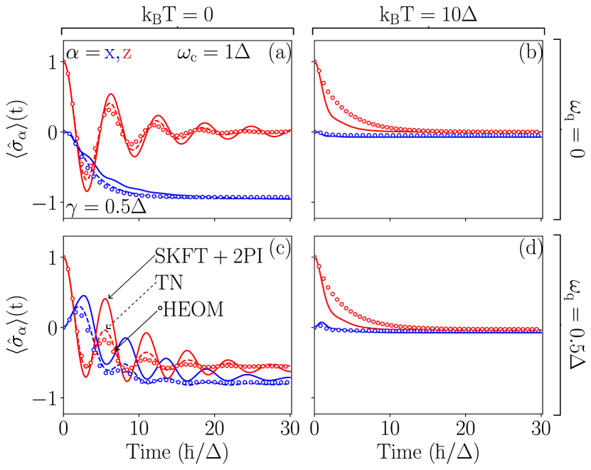
The spin-boson model describes quantum spin interacting with a bosonic bath as the dissipative environment. Although SKFT+2PI approach has been applied to a closed system of quantum spins [22, 21], it has never been benchmarked against numerically exact methods available in low dimensions. In fact, since diagrams missed by 2PI resummation act as an additional dissipative environment, it is more natural to apply SKFT+2PI approach to open quantum systems and contrast its results with well-known techniques [27, 28, 29, 30, 31, 32, 33, 34, 35, 36, 37, 38, 6, 33, 39]. In particular, we benchmark SKFT+2PI against Lindblad QME in the Markovian regime, and against hierarchical equations of motion (HEOM) [40] and tensor network (TN)-based methods [6, 39, 33] in the non-Markovian regime. Our principal results in Figs. 4 and 5 demonstrate that SKFT+2PI can mimic results of all three standard methods, while being able to treat spin-boson model at zero temperature, strong coupling, and with differing bath spectral densities. Handling these combinations of features poses an intractable challenge for presently available HEOM and TN-based algorithms.
The paper is organized as follows. The spin-boson model and standard approaches for its treatment are overviewed in Sec. II.1. In Sec. II.2 we introduce SKFT+2PI approach for open quantum system dynamics. We provide details of our TN-based, HEOM and Lindblad QME reference calculations in Secs. II.3, II.4 and II.5, respectively. We compare SKFT+2PI results in Sec. III and Figs. 4 and 5. We conclude in Sec. IV.
II Models and methods
II.1 Spin-boson model
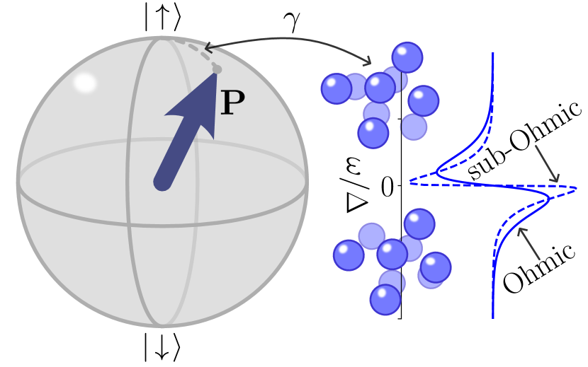
The spin-boson model is a two-level quantum system—as realized by a spin , a qubit [19, 20], or any two well-separated energy levels [2, 3]—which is made open by its interaction with a bosonic bath composed of infinitely many harmonic oscillators [9]. Although it has been intensely studied for nearly four decades [9], its non-Markovian dynamics [5, 6, 2, 41, 42] still pose a formidable challenge despite the plethora of available numerical and analytical methods [27, 28, 29, 30, 31, 32, 33, 34, 35, 36, 37, 38, 6, 33, 39, 43, 44, 45, 46, 47] for open quantum systems. This is especially true for the case of zero [38, 30, 42] or ultralow temperatures and/or specific frequency content of the bosonic bath [41, 30]. This is of particular relevance to superconducting qubits [19, 20], where ultralow temperatures and sub-Ohmic bath model such qubit subject to electromagnetic noise [45]. The zero or ultralow temperature makes strong quantum effects and long memory time of the bath pronounced, while transition from coherent damped motion to localization is generated by increasing the system-bath coupling strength.
The total system-bath Hamiltonian of spin-boson model is given by
| (1) |
where for simplicity of notation; is the vector of the Pauli operators; is the energy difference between the two eigenstates of , ; is the tunneling matrix element, which sets the units of energy; and are bosonic creation and annihilation operators, respectively; and the spin is coupled with strength to the -th mode of the bath via the fourth term in Eq. (1). The impact of the bath on the spin is fully captured by the coupling-weighted spectral density, , for which a generic form
| (2) |
is usually assumed [9]. Here is the parameter characterizing spin-bath coupling strength; is the characteristic or cutoff frequency of the bath; parameter , and classifies spectral densities as sub-Ohmic, Ohmic and super-Ohmic, respectively [30]; and the spectral density is antisymmetrically extended [27].
The sub-Ohmic case, with a relatively large portion of low-frequency modes, is considered as particularly challenging [30, 35, 43, 44, 45, 46] at zero temperature (). This also includes the hurdle posed by the long-time limit [30, 48, 35, 36] of non-Markovian dynamics [41, 42], whose memory effects force information to flow from the environment back to the system and such effects are not necessarily transient [41]. It is generally believed that non-Markovian regime [5, 6, 2] in open quantum system dynamics is entered when the system-bath coupling is sufficiently strong and correlations of the bath do not decay rapidly [7]. But detailed examination [41, 42] of measures of non-Markovianity vs. system-bath coupling strength in the case of spin-boson model shows complex (nonmonotonic) dependence, including sensitivity on the cutoff frequency . In the non-Markovian regime, one finds recoherence effects and a departure from purely exponential decay in the dynamics of system observables, as illustrated in the spin-boson model by comparing Markovian and non-Markovian dynamics in Figs. 4 vs. 5, respectively.
The brute force numerical solution of QME in the non-Markovian regime requires computing high-dimensional integrals over time [49], where accuracy of calculations become extremely sensitive to numerical errors. The widely-used HEOM approach [50, 40] converts time-nonlocal integro-differential QME of the brute force method [49] into a set of finitely many time-local differential equations. However, its standard version [40] is limited to high temperatures [51], which is a problem only very recently tackled by extending HEOM approach [48, 35, 36] to access zero temperature and much longer simulation times. Multilayer multiconfiguration time-dependent Hartree (ML-MCTDH) [29, 30], numerical renormalization group (NRG) [43, 44, 45, 46] and TN-based [32, 33, 34, 38, 39, 6] algorithms that can handle non-Markovian regime have also been developed. But, typically, TN-based approaches are limited to short time evolution. In addition, HEOM and ML-MCTDH algorithms would be prohibitively expensive for many interacting quantum spins or, equivalently, qubits. Although TN-based approaches can handle many interacting quantum spins, they are also prohibitively expensive in higher dimensions or when time evolution exhibits a transient “entanglement barrier” [52, 53]. For example, even Markovian dynamics can lead to a spike [54] in time evolution of many-body entanglement of the system, despite the presence of dissipative environment and naïve expectation [55] that interactions with the environment should curtail entanglement growth. Thus, the need for new approaches for driven-dissipative systems of many locally interacting quantum spins motivates development of SKFT-based theory in Sec. II.2, as a highly credible route (thus far demonstrated only for closed quantum systems [21, 22]) for computing the dynamics of many quantum degrees of freedom in arbitrary spatial dimension that is also capable of evolving such systems over long times.
II.2 Schwinger-Keldysh field theory + 2PI for both Markovian and non-Markovian dynamics
Formulating the functional integral of SKFT is cumbersome due to spin operator commutation relations, which are neither bosonic nor fermionic. Instead, it is convenient to map the spin operators in the Hamiltonian of Eq. (1) onto fermionic or bosonic operators [56], so that the Wick theorem and field-theoretic machinery applicable to such operators can be utilized. Here we employ the Schwinger boson representation [57, 58, 22], in which the spin operators are expressed as
| (3) |
where ; is a matrix representation of the Pauli operators; and is a doublet of the two Schwinger bosons, and . The total spin constrains the number of bosons to be . The constraint ensures that only a subspace of the infinite dimensional bosonic Hilbert space is utilized for spin dynamics, such as which span the physical Hilbert space of spin . Unlike imaginary time applications of Schwinger bosons [58, 57], the conserved currents associated with the symmetries of the SK action enforce this constraint throughout real time evolution [22]. Although other mappings from spin to bosons or fermions can be employed, Schwinger bosons preserve rotational symmetry, as opposed to Holstein-Primakoff bosons [59], and are generalizable to larger spin value, unlike Majorana [21] or Jordan-Wigner [60] fermions applicable only to . Thus, we adopt Schwinger bosons, akin to Ref. [22] which applied them to develop SKFT for many quantum spins, of arbitrary spin value and in arbitrary spatial dimension, but viewed as a closed quantum system (i.e., no dissipative environment appears in Ref. [22], or Ref. [21], where SKFT is formulated for spins using their mapping to Majorana fermions).
The SK functional integral is formulated in terms of complex fields which are eigenvalues, of and are the bosonic coherent states. Real fields can be extracted from by switching to real and imaginary components, and , grouped into the 4-component field . The spin fields can be constructed as , where
| (4) |
and is the 22 identity matrix.
Then the SK action, , as one of the central quantities in SKFT, is obtained as
| (5a) | ||||
| (5b) | ||||
by time evolving the Lagrangian corresponding to the Hamiltonian in Eq. (1) along the SK closed time contour [13, 14, 15, 16]. Here and are the contributions to the total action from the system and the bath, respectively; ; and . The action of the bath is already in the Gaussian form, so it can be integrated out exactly. This leaves behind a quartic term in the total action, representing a nonlocal-in-time effective self-interaction of the spin generated by the presence of the bath. The bath kernel is given in terms of the Keldysh Green’s functions (GFs) of the bosonic bath, , where there are four of them [13] because of four possibilities for placing the times on the forward and backward branches of the SK contour . The quartic term can be decoupled through a Hubbard-Stratonovich transformation [61], yielding the modified total action
| (6) | ||||
where is the Hubbard-Stratonovich field that mediates the nonlocal-in-time effective interaction.
To progress from the modified total action in Eq. (6), several routes are possible. For instance, the quantum (for the bath)-classical (for the spin) regime can be probed by minimizing the action with respect to quantum fluctuations that emerge naturally from the SK closed time contour, thereby yielding integro-differential equations of motion for the fields that contain time-retarded (i.e., non-Markovian) dissipation kernel accounting for the bath [62, 63, 64, 12]. The form of these equations [65, 66] is quite analogous to the Nakajima-Zwanzig equation [67, 68]. The time-retarded kernel can be either approximated by analytical means [62, 64], or solved numerically exactly [63]. Note that in the quantum-classical regime, the memory of the bath is encoded in the dissipation kernel, which is a feature completely missed in SKFT description of open quantum systems where Markovianity is built into the SK functional integral [69, 12, 17]. Alternatively, the fully quantum regime can be captured from the action in Eq. (6) by deriving the Dyson equations for the -particle correlation functions [13, 16]. However, an additional scheme is required in order to handle the self-consistent nature of the ensuing self-energy and approximate it in a controllable manner. Here, we borrow from elementary particle physics [16] the 2PI effective action formalism [14, 70] which sums [23] an infinite number of Feynman diagrams of particular topology where the coupling constant in the diagrammatic perturbation theory is [71, 72, 73, 22, 21, 74, 75], being the number of Schwinger bosons in our SKFT reformulation of the spin-boson model. This can then lead to nonperturbative results in the system-bath coupling , as demonstrated in Fig. 5 where dynamics considering such subset of all possible diagrams follows remarkably closely what are considered numerically exact benchmarks (as obtained from HEOM and TN-based calculations) in the field.
The 2PI effective action is obtained from the connected generating functional
| (7) | ||||
where indicates functional integration over all possible configurations of five-component field , and and are one- and two-particle sources [16, 22], respectively. The Legendre transform of the functional with respect to both arguments is the 2PI effective action
| (8) | ||||
Here, and are the one- and two-particle connected expectation values generated by . That is, is the expectation value of the fields and is the connected Keldysh GF. Although both and hold the same information, the former produces expectation values via functional derivatives in the limit of vanishing sources, whereas the latter produces them through a comparatively simpler variational approach—the expectation values satisfy and . Such variational calculations can be performed on the expansion [26]
| (9) |
where a constant term has been ignored; the trace is taken over all possible indices and times; is the inverse of the free Keldysh GF (i.e., for spin and bath decoupled from each other); and contains all the 2PI vacuum diagrams. These 2PI vacuum diagrams are those that cannot be separated by cutting two edges or fewer, with edges (i.e., Keldysh GF ) and vertices corresponding to interactions contained in the action .
The spin-to-Schwinger-boson mapping implies that any expectation value containing an odd number of Schwinger bosons vanishes in the physical states. In particular, and . Therefore, the equations of motion obtained from the expansion of the 2PI action in Eq. (9) via variational principle are given by
| (10a) | ||||
| (10b) | ||||
| (10c) | ||||
where and are the connected Keldysh GFs; and are the self-energies derived through functional differentiation of the 2PI vacuum diagrams; ; ; and summation over repeated indices is implied. Equations (10) do not form a closed system of equations that can be solved due to the infinite diagrammatic summation within the self-energies, so a controlled approximation scheme is required.
One possibility is to neglect , which leads to quantum-classical spin dynamics of the Landau-Lifshitz-Gilbert type [62, 64, 63]. For fully quantum dynamics, the diagrammatic expansion of needs to be truncated. We adopt the scheme used in Ref. [22], where diagrams are truncated based on powers of the inverse of the number of Schwinger bosons , which has been previously shown to adequately capture the relevant features of closed quantum system [73, 22]. Surprisingly, such expansions have been successful even when is not small, such as for [72, 71] that we use here, or in different mappings of spin to fermionic operators [21]. Each diagram in the expansion is made up of vertices,
| (11) |
where outgoing solid (dashed) lines correspond to a Schwinger boson field (Hubbard-Stratonovich field ). Within a particular diagram, closed loops of solid lines scale proportional to the number of Schwinger bosons due to being traces over this space, while dashed lines scale as . This can be inferred from the action in Eq. (6), where , and the equation of motion for [Eq. (10b)] because . Thus, the 2PI diagram with the lowest scaling is the two loop one:
| (12) | ||||
At this order, the corresponding self-energies are given by
| (13a) | ||||
| (13b) | ||||
Note that all the lines of 2PI diagram in Eq. (12) are dressed or fully interacting, Keldysh GFs, which already contain an infinite series of diagrams in terms of the bare noninteracting Keldysh GFs. The self-consistency [23] built into 2PI resummation evades [76] the so-called secularity problem for expansion in terms of the bare Keldysh GFs, where elapsed time appearing next to the coupling constant makes the effective coupling arbitrarily large at late times. The same self-consistency ensures that all global conservation laws are satisfied [77].
Equations (10) and (13) are defined on the SK closed time contour and are, therefore, complex. The real time equations are obtained by decomposing the contour GFs [14] as . The statistical and spectral parts of the Keldysh GFs are in turn related to the lesser and greater GFs, commonly employed in operator formulation of Keldysh GFs [77]. The arguments of and take values in real time, while the sign function equals 1 if its arguments are ordered on the contour or vice versa. Through this decomposition, integrals over simplify to real time integrals (which in operator language requires handling the much more demanding Langreth rules [77, 78]) that preserve causality, yielding equations of motion
| (14a) | ||||
| (14b) | ||||
| (14c) | ||||
| (14d) | ||||
| (14e) | ||||
| (14f) | ||||
| (14g) | ||||
| (14h) | ||||
| (14i) | ||||
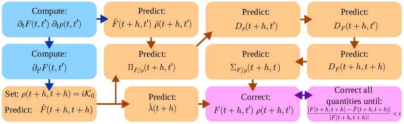
Here, the subscripts and signify that the respective quantity with such subscript is the statistical or spectral part, respectively, of the original quantity defined on the SK contour . These nine coupled equations form an integro-differential system of the Volterra type [79]. They must be integrated carefully due to the self-consistent interdependence between nine functions whose solution is required to finally obtain , which yields the spin expectation values in Figs. 4 and 5. For this purpose, we discretize both time arguments and , and we employ a predictor-corrector algorithm [see Fig. 2 for a flow chart describing the numerical implementation]. Note that all functions satisfy , so that calculations at times are sufficient. We first compute the right-hand side (RHS) of Eqs. (14a) and (14b) plugging in the functions at the current time step and . Then, we predict the functions at the next time step as, e.g., . Predicting the diagonal time step, i.e., , requires the derivative with respect to the second time argument, , obtained from the transpose of Eq. (14a) and the symmetry properties of the Keldysh GFs. The time-diagonal of is fixed by the equal-time commutation relations of the real Schwinger bosons, so we set it to . All integrals are discretized using the trapezoid method and identical time increment . Predictions for all subsequent functions are obtained in the order shown in Fig. 2, starting with plugging into Eqs. (14g) and (14h). The predictions for all functions are then used to recompute the RHS of Eqs. (14a) and (14b) to get . The correction step is repeated, by using and as new predictions, until the relative difference between the predicted and corrected diagonal time steps of are below a certain tolerance [see lower right corner of the flow chart in Fig. 2].
II.3 Tensor network approach to non-Markovian dynamics
For low temperatures, we use a TN approach, as implemented in terms of matrix product states (MPSs), to benchmark [Figs. 4(a),(c) and 5(a),(c)] our results from SKFT+2PI. An MPS is a representation of an arbitrary pure state as a product of local tensors given by [80]
| (15) |
where is a matrix (with fixed) for the th local degree of freedom possessing a dimensional Hilbert space.
In order to represent the equilibrium state of the bath in the form of a pure state MPS, we use thermofield purification in which the finite temperature of the bath is encoded in two different baths at zero temperature [81]. The thermal state of a bosonic bath at inverse temperature is given by
| (16) |
where By introducing an identical auxillary system with canonical operators we can define the thermofield double state as a purification of , given by
| (17) |
where is bosonic vacuum state; ; and is obtained by partial trace over the states of auxiliary system . The state is the vacuum for the modes
| (18) | ||||
| (19) |
where is a thermal Bogoliubov transformation. We then use as the ancilla system Hamiltonian such that in the new basis the extended Hamiltonian is given by
| (20) |
where and .
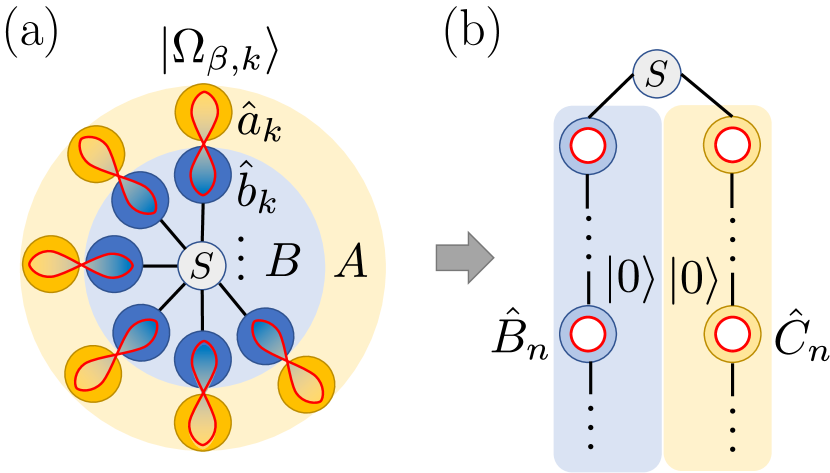
As it stands, this setup has a star geometry in which the spin interacts with each eigenmode of the bath, as illustrated graphically in Fig. 3(a). Within the one-dimensional connectivity of an MPS, this corresponds to long-ranged interactions, which are more difficult to handle in this formalism. For this reason, we map via continuous mode tridiagonalization the two zero temperature star geometry baths into two one-dimensional tight binding chains, each coupled to the system spin [6], as shown in Fig. 3(b). In the continuum representation, these two baths are characterized by spectral densities and where is the Bose-Einstein distribution function, which we use to define new bosonic operators and such that
| (21) |
Here, for and are monic orthogonal polynomials that obey , with [39]. This description simplifies significantly at zero temperature, as , so only one chain is needed. Using a finite cutoff of modes for the mapping, we have
| (22) |
where the coefficients and are defined through the recurrence relation , with . These chain parameters were generated using the ORTHPOL package [82]. Generically, they are found to quickly converge to constants , . Using the Lieb-Robinson bounds [83], sites further than have a negligible effect on the system dynamics up to time , giving a well-defined measure of the length of bath chains we need. In this sense, the discretization generated by orthogonal polynomials is exact up to a finite time. To time evolve the MPS, we use the two-site variant of the time dependent variational principle (TDVP) [84, 85, 86, 87] which dynamically updates the MPS bond dimensions to maintain a desired level of precision.
II.4 HEOM approach to non-Markovian dynamics
The HEOM algorithm [40], initially developed for problems in quantum chemistry [50], is a widely used method for solving QMEs of open quantum systems with arbitrary system-bath coupling. However, in its original formulation [50, 40] it requires finite temperature, [51, 48, 35, 36]. The non-perturbative treatment of interaction with the bath is achieved by introducing a hierarchy of auxiliary density matrices which encode system-bath correlations and entanglement [40, 88]. This hierarchy relies on the expansion of the bath correlation function into an exponential form. The limitations of the HEOM method are well known [51, 48, 35, 36] and arise from the truncation of either the number of auxiliary matrices (a stronger system-bath coupling requires a higher hierarchy cutoff), or the truncation in the exponential decomposition of the bath correlation (typically, lower temperature requires a higher number of terms in the expansion). The exact exponential expansion of an arbitrary spectral density of the bath is not known. We fit the spectral density in Eq. (2) using a sum of up to four underdamped [40] spectral densities whose exponential expansion is well known [89]. In order to guarantee convergence, we ran simulations varying the hierarchy cutoff, such as by considering up to 11 auxiliary density matrices. In addition, we also adjust the number of exponential terms, using a maximum of 16 terms for the lowest temperature case [Fig. 5]. All such calculations were performed using the HEOM extension [90] of the QuTiP [91, 92] package.
II.5 Lindblad QME approach to Markovian dynamics

In the weak system-bath coupling regime, where the system (i.e., spin) dynamics is expected to be Markovian [41, 42], it is assumed that Lindblad QME [4, 7]
| (23) |
can accurately capture the open quantum system dynamics. Here is the Hamiltonian of an isolated spin, composed of the first two terms on the RHS of Eq. (1); is the spin density matrix [10]; and is a set of three Lindblad operators [4, 7] which account for the presence of the bosonic bath. Those three operators for the spin-boson model can be expressed [1] in the energy eigenbasis of , , of as
| (24a) | ||||
| (24b) | ||||
| (24c) | ||||
where is the energy difference of the two levels; is the system-bath coupling we have to adjust [Fig. 4] when using Lindblad QME; and is the Bose-Einstein distribution.
III Results and discussion
The dynamics of spin expectation values
| (25) |
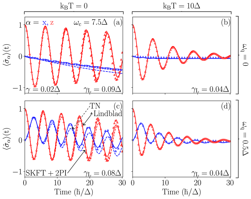
is plotted in Figs. 4 and 5 for the Ohmic bath, and in 6 for sub-Ohmic bath. In Fig. 4 we focus on the Markovian regime. Note that delineating precise boundary between Markovian and non-Markovian regimes requires considering [41, 42] the interplay of several parameters in the spin-boson model. Nevertheless, the most important ones are the strength of the system-bath coupling and the cutoff frequency [7]. Therefore, in Fig. 4 we employ small and high . The Markovian nature of such regime is reflected in the irreversible decay of purity [orange solid line in Fig. 7] of the mixed quantum state of spin. Since the spin density matrix and the Bloch vector are in one-to-one correspondence [10],
| (26) |
where is the unit operator in the spin space, we use as the purity. The standard purity is a function of , where signifies fully coherent or pure quantum state of spin or qubit. In the Markovian regime, we find excellent agreement between SKFT+2PI (solid lines) and Lindblad-QME-computed results (triangles) in Fig. 4. However, such a match is ensured only by adjusting the system-bath coupling in the Lindblad QME, which points to an artifact of standard Lindblad QME [1] since SKFT+2PI also closely matches the resutls of TN-based approach (dashed lines in Figs. 4 and 5) employing the same coupling . Outside the Markovian regime, the Lindblad QME does not capture the memory effects of the bath, which can cause the revival of quantum properties. Such revival is exemplified by the purity of the mixed quantum state of spin initially decaying in Figs. 7(a) and 7(c), as the signature of decoherence [11], but later it starts to increase toward of the pure state at as the signature of recoherence [2].
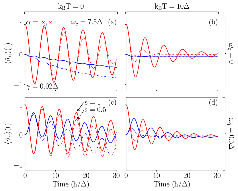
In the non-Markovian regime of Fig. 5, we therefore switch the benchmarking from Lindblad QME to HEOM and TN-based approaches expected to provide numerically exact results. The non-Markovian regime [Fig. 5] is induced by using strong system-bath coupling and low cutoff frequency , while keeping Ohmic bath as in Fig. 4. We find that for zero temperature [Figs. 5(a),(c)], the TN-computed results (dashed lines in Fig. 5) follow closely those from HEOM (circles in Fig. 5), on the proviso that we use slightly higher temperature in the HEOM calculations as the standard version of this approach cannot [48, 35, 36] handle . The spin expectation values computed from our SKFT+2PI are quite capable in mimicking these benchmark results, but they appear as if their damping is slightly smaller [Figs. 5(c)]. This goes against naïve expectation of higher damping effectively emerging [73, 79] in closed quantum systems due to neglected Feynman diagrams in 2PI resummation.
Finally, Fig. 6 demonstrates the ability of SKFT+2PI to treat a variety of other system and bath parameters, such as the case of zero temperature and sub-Ohmic bath that is considered particularly challenging [30, 35, 43, 44, 45, 46]. For this purpose, we compute via SKFT+2PI the spin expectation values for a sub-Ohmic bath with in Eq. (2) while using the same parameters as in the weak system-bath coupling regime of Fig. 4 for the sake of comparing Ohmic vs. sub-Ohmic cases. The results [Fig. 6] show faster decrease of the spin expectation values when the bath is sub-Ohmic. However, the purity in sub-Ohmic case [orange dotted line in Fig. 7] does not decay monotonically as in the case of Markovian regime for Ohmic bath [orange solid line in Fig. 7]. Instead, it saturates at a finite value at zero temperature, akin to the Ohmic non-Markovian case [green line in Fig. 7 obtained using SKFT+2PI from Fig. 5]. Moreover, at high temperature, it closely resembles the time evolution of the purity in the strong system-bath coupling, non-Markovian regime except for small revivals [orange dotted curve in Figs. 7(b),(d)] at intermediate time scales. Thus, Fig. 7 illustrates the difficulties [30, 35, 43, 44, 45, 46] posed by the sub-Ohmic case because of the skew towards low bath frequencies [Fig. 1] which enhances the memory effects of the bath, thereby allowing for the non-Markovian features to show up despite weak system-bath coupling. In other words, standard notion that system-bath coupling is the primary controller of the boundary between Markovian and non-Markovian regimes, with low temperature making the non-Markovian effects more pronounced [29, 30, 38], requires careful reexamination as the spin-boson model can exhibit complex regime diagram [41, 42] due to interplay of several parameters in Eqs. (1) and (2). Thus, we find weak system-bath coupling and a sub-Ohmic bath [Fig. 6] can be as challenging as strong system-bath coupling and an Ohmic bath [Fig. 5], but SKFT+2PI provides relatively easy access to many different combinations of parameters, as well as for long evolution time.
IV Conclusions and outlook
In conclusion, we demonstrate a promissing new avenue for theoretical modeling of driven-dissipative many-body systems [93], while focusing on the system composed of spins or qubits, as one of the most challenging unsolved problems in many-body quantum physics. Although this problem could be solved with rapid improvements in quantum hardware and algorithms [93], presently available algorithms for classical computers face challenges with increasing number of degrees of freedom (such as HEOM solution of non-Markovian QMEs or NRG methods) or increasing simulation time and spatial dimensionality (such as TN methods due to inability to handle transient entanglement barrier [52]). On the other hand, our SKFT+2PI approach integrates out dissipative environment via SK functional integral techniques leaving the open system composed of quantum spins of arbitrary value . This provides nonperturbative solution in terms of system-bath coupling, as well as for arbitrary temperature and cutoff frequency of the bath spectral density. This is achieved by employing 2PI resummation [26, 16, 21, 22] of a class of infinitely many Feynman diagrams in the perturbative expansion in , for being the number of Schwinger bosons to which quantum spins are mapped, rather than in the system-bath coupling in terms of which our solution remains nonperturbative.
We recall that SKFT+2PI has been applied before to closed quantum systems of many spins [21, 22] or cold atoms [73, 94]. SKFT alone has been developed for open quantum systems, but only in the Markovian regime [12, 17, 13] as an alternative to standard Lindblad QME where it offers numerical efficiency with increasing number of degrees of freedom [17] and a toolbox of field-theoretical techniques (such as renormalization group [12, 95]). However, SKFT formulation of non-Markovian regime of open quantum systems has been lacking. Also, benchmarking [73] of SKFT+2PI applied to close quantum systems against numerically exact solutions (available for sufficiently small number of degrees of freedom) can reveal significant discrepancy because Feynman diagrams not taken into account by 2PI resummation [23] act effectively as an implicit dissipative environment which is damping expectation values of physical quantities shortly after the initial match between SKFT+2PI and numerically exact dynamics. Thus, it seems more natural to apply SKFT+2PI to systems containing dissipative environment explicitly, as demonstrated by the excellent match of our results in Figs. 4 and 5 to standard techniques (i.e., HEOM and TN-based) for solving archetypical spin-boson model. In other words, our formulation of SKFT+2PI for open quantum systems in arbitrary regime suggests that neglected Feynman diagrams are somehow masked by the presence of real dissipative environment. Furthermore, if higher accuracy is desired, SKFT+2PI can be systematically improved by: combining 2PI with additional resummation [23, 25]; including more loops [96] within 2PI self-consistent diagram [beyond the two shown in Eq. (12)]; or going to PI resummation [97, 96]. Unlike previously developed techniques that can hardly be scaled to more degrees of freedom (such as HEOM [40, 51], ML-MCTDH [29, 30] or NRG [43, 44, 45, 46]) or longer time (such as TN-based approaches [32, 33, 34, 38, 39, 6]), our SKFT+2PI formalism can make progress in both of these directions while also offering relatively easy access to arbitrary system or bath parameters and temperature. Therefore, we relegate to future studies demonstration of SKFT+2PI-based simulations on extensions of spin-boson model, i.e., for many quantum spins coupled to different types of dissipative environments. This is a problem in “high demand” for quantum spintronics [98] and magnonics [99], where the spin value , as well as for emulation of quantum hardware where for qubits. Such simulations will be greatly facilitated by the numerical cost of solving integro-differential equations [Eq. (14) and Fig. 2] produced by SKFT+2PI approach, which is quartic scaling in the number of time steps, but it could be lowered to linear by optimizing numerics, and the need to handle matrices of size (instead of matrices in brute force methods) for spins of arbitrary value .
Acknowledgements.
We are grateful to L. E. Herrera Rodríguez for technical help regarding intricacies of HEOM calculations. F. R.-O., B. K. N. and F. G.-G. were supported by the US National Science Foundation through the University of Delaware Materials Research Science and Engineering Center, Grant No. DMR-2011824. Work of P.P. was partially supported by the U.S. Army Research Office Grant W911NF-22-2-0234. S.R.C. gratefully acknowledges financial support from UK’s Engineering and Physical Sciences Research Council (EPSRC) under grant EP/T028424/1.References
- Breuer and Petruccione [2007] H.-P. Breuer and F. Petruccione, The Theory of Open Quantum Systems (Oxford University Press, Oxford, 2007).
- Breuer et al. [2016] H.-P. Breuer, E.-M. Laine, J. Piilo, and B. Vacchini, Colloquium: Non-Markovian dynamics in open quantum systems, Rev. Mod. Phys. 88, 021002 (2016).
- de Vega and Alonso [2017] I. de Vega and D. Alonso, Dynamics of non-Markovian open quantum systems, Rev. Mod. Phys. 89, 015001 (2017).
- Lindblad [1976] G. Lindblad, On the generators of quantum dynamical semigroups, Commun. Math. Phys. 48, 119 (1976).
- Rivas et al. [2014] A. Rivas, S. F. Huelga, and M. B. Plenio, Quantum non-Markovianity: characterization, quantification and detection, Rep. Prog. Phys. 77, 094001 (2014).
- de Vega and Bañuls [2015] I. de Vega and M.-C. Bañuls, Thermofield-based chain-mapping approach for open quantum systems, Phys. Rev. A 92, 052116 (2015).
- Nathan and Rudner [2020] F. Nathan and M. S. Rudner, Universal Lindblad equation for open quantum systems, Phys. Rev. B 102, 115109 (2020).
- Prosen [2008] T. Prosen, Third quantization: a general method to solve master equations for quadratic open Fermi systems, New Journal of Physics 10, 043026 (2008).
- Leggett et al. [1987] A. J. Leggett, S. Chakravarty, A. T. Dorsey, M. P. A. Fisher, A. Garg, and W. Zwerger, Dynamics of the dissipative two-state system, Rev. Mod. Phys. 59, 1 (1987).
- Ballentine [2014] L. E. Ballentine, Quantum Mechanics: A Modern Development (World Scientific, Singapore, 2014).
- Joos et al. [2003] E. Joos, H. D. Zeh, C. Kiefer, D. Giulini, J. Kupsch, and I.-O. Stamatescu, Decoherence and the Appearance of a Classical World in Quantum Theory (Springer, Berlin Heidelberg, 2003).
- Sieberer et al. [2016] L. M. Sieberer, M. Buchhold, and S. Diehl, Keldysh field theory for driven open quantum systems, Rep. Prog. Phys. 79, 096001 (2016).
- Kamenev [2023] A. Kamenev, Field Theory of Non-Equilibrium Systems (Cambridge University Press, Cambridge, 2023).
- Berges [2015] J. Berges, Nonequilibrium quantum fields: From cold atoms to cosmology, arXiv:1503.02907 (2015).
- Calzetta and Hu [2008] E. A. Calzetta and B.-L. B. Hu, Nonequilibrium Quantum Field Theory (Cambridge University Press, Cambridge, 2008).
- Gelis [2019] F. Gelis, Quantum Field Theory: From Basics to Modern Topics (Cambridge University Press, Cambridge, 2019).
- Thompson and Kamenev [2023] F. Thompson and A. Kamenev, Field theory of many-body Lindbladian dynamics, Ann. Phys. 455, 169385 (2023).
- Maghrebi and Gorshkov [2016] M. F. Maghrebi and A. V. Gorshkov, Nonequilibrium many-body steady states via Keldysh formalism, Phys. Rev. B 93, 014307 (2016).
- Gulácsi and Burkard [2023] B. Gulácsi and G. Burkard, Signatures of non-Markovianity of a superconducting qubit, Phys. Rev. B 107, 174511 (2023).
- Rossini et al. [2023] M. Rossini, D. Maile, J. Ankerhold, and B. I. C. Donvil, Single-qubit error mitigation by simulating non-Markovian dynamics, Phys. Rev. Lett. 131, 110603 (2023).
- Babadi et al. [2015] M. Babadi, E. Demler, and M. Knap, Far-from-equilibrium field theory of many-body quantum spin systems: Prethermalization and relaxation of spin spiral states in three dimensions, Phys. Rev. X 5, 041005 (2015).
- Schuckert et al. [2018] A. Schuckert, A. Orioli, and J. Berges, Nonequilibrium quantum spin dynamics from two-particle irreducible functional integral techniques in the Schwinger boson representation, Phys. Rev. B 98, 224304 (2018).
- Brown and Whittingham [2015] M. Brown and I. Whittingham, Two-particle irreducible effective actions versus resummation: Analytic properties and self-consistency, Nucl. Phys. B 900, 477 (2015).
- Mera et al. [2016] H. Mera, T. G. Pedersen, and B. K. Nikolić, Hypergeometric resummation of self-consistent sunset diagrams for steady-state electron-boson quantum many-body systems out of equilibrium, Phys. Rev. B 94, 165429 (2016).
- Mera et al. [2018] H. Mera, T. G. Pedersen, and B. K. Nikolić, Fast summation of divergent series and resurgent transseries from Meijer- approximants, Phys. Rev. D 97, 105027 (2018).
- Cornwall et al. [1974] J. M. Cornwall, R. Jackiw, and E. Tomboulis, Effective action for composite operators, Phys. Rev. D 10, 2428 (1974).
- Makri [1995] N. Makri, Numerical path integral techniques for long time dynamics of quantum dissipative systems, J. Math. Phys. 36, 2430 (1995).
- Winter et al. [2009] A. Winter, H. Rieger, M. Vojta, and R. Bulla, Quantum phase transition in the sub-Ohmic spin-boson model: Quantum Monte Carlo study with a continuous imaginary time cluster algorithm, Phys. Rev. Lett. 102, 030601 (2009).
- Wang and Thoss [2008] H. Wang and M. Thoss, From coherent motion to localization: dynamics of the spin-boson model at zero temperature, New J. Phys. 10, 115005 (2008).
- Wang and Thoss [2010] H. Wang and M. Thoss, From coherent motion to localization: II. dynamics of the spin-boson model with sub-Ohmic spectral density at zero temperature, Chem. Phys. 370, 78 (2010).
- Strathearn et al. [2017] A. Strathearn, B. W. Lovett, and P. Kirton, Efficient real-time path integrals for non-Markovian spin-boson models, New J. Phys. 19, 093009 (2017).
- Strathearn et al. [2018] A. Strathearn, P. Kirton, D. Kilda, J. Keeling, and B. W. Lovett, Efficient non-Markovian quantum dynamics using time-evolving matrix product operators, Nat. Commun. 9, 3322 (2018).
- Ye and Chan [2021] E. Ye and G. K.-L. Chan, Constructing tensor network influence functionals for general quantum dynamics, J. Chem. Phys. 155, 044104 (2021).
- Cygorek et al. [2022] M. Cygorek, M. Cosacchi, A. Vagov, V. M. Axt, B. W. Lovett, J. Keeling, and E. M. Gauger, Simulation of open quantum systems by automated compression of arbitrary environments, Nat. Phys. 18, 662 (2022).
- Xu and Ankerhold [2023] M. Xu and J. Ankerhold, About the performance of perturbative treatments of the spin-boson dynamics within the hierarchical equations of motion approach, Eur. Phys. J. Spec. Top. 232, 3209–3217 (2023).
- Xu et al. [2023] M. Xu, V. Vadimov, M. Krug, J. T. Stockburger, and J. Ankerhold, A universal framework for quantum dissipation: Minimally extended state space and exact time-local dynamics, arXiv:2307.16790 (2023).
- Weber [2022] M. Weber, Quantum Monte Carlo simulation of spin-boson models using wormhole updates, Phys. Rev. B 105, 165129 (2022).
- Vilkoviskiy and Abanin [2023] I. Vilkoviskiy and D. A. Abanin, A bound on approximating non-Markovian dynamics by tensor networks in the time domain, arXiv:2307.15592 (2023).
- Chin et al. [2010] A. W. Chin, A. Rivas, S. F. Huelga, and M. B. Plenio, Exact mapping between system-reservoir quantum models and semi-infinite discrete chains using orthogonal polynomials, J. Math. Phys. 51, 092109 (2010).
- Tanimura [2020] Y. Tanimura, Numerically “exact” approach to open quantum dynamics: The hierarchical equations of motion (HEOM), J. Chem. Phys. 153, 020901 (2020).
- Clos and Breuer [2012] G. Clos and H.-P. Breuer, Quantification of memory effects in the spin-boson model, Phys. Rev. A 86, 012115 (2012).
- Wenderoth et al. [2021] S. Wenderoth, H.-P. Breuer, and M. Thoss, Non-Markovian effects in the spin-boson model at zero temperature, Phys. Rev. A 104, 012213 (2021).
- Bulla et al. [2003] R. Bulla, N.-H. Tong, and M. Vojta, Numerical renormalization group for bosonic systems and application to the sub-ohmic spin-boson model, Phys. Rev. Lett. 91, 170601 (2003).
- Anders and Schiller [2006] F. B. Anders and A. Schiller, Spin precession and real-time dynamics in the Kondo model: Time-dependent numerical renormalization-group study, Phys. Rev. B 74, 245113 (2006).
- Anders et al. [2007] F. B. Anders, R. Bulla, and M. Vojta, Equilibrium and nonequilibrium dynamics of the sub-Ohmic spin-boson model, Phys. Rev. Lett. 98, 210402 (2007).
- Vojta [2012] M. Vojta, Numerical renormalization group for the sub-Ohmic spin-boson model: A conspiracy of errors, Phys. Rev. B 85, 115113 (2012).
- Orth et al. [2013] P. P. Orth, A. Imambekov, and K. Le Hur, Nonperturbative stochastic method for driven spin-boson model, Phys. Rev. B 87, 014305 (2013).
- Xu et al. [2022] M. Xu, Y. Yan, Q. Shi, J. Ankerhold, and J. T. Stockburger, Taming quantum noise for efficient low temperature simulations of open quantum systems, Phys. Rev. Lett. 129, 230601 (2022).
- Shibata and Arimitsu [1980] F. Shibata and T. Arimitsu, Expansion formulas in nonequilibrium statistical mechanics, J. Phys. Soc. Japan 49, 891 (1980).
- Tanimura and Wolynes [1991] Y. Tanimura and P. G. Wolynes, Quantum and classical Fokker-Planck equations for a Gaussian-Markovian noise bath, Phys. Rev. A 43, 4131 (1991).
- Xu et al. [2017] M. Xu, L. Song, K. Song, and Q. Shi, Convergence of high order perturbative expansions in open system quantum dynamics, J. Chem. Phys. 146, 064102 (2017).
- Lerose et al. [2023] A. Lerose, M. Sonner, and D. A. Abanin, Overcoming the entanglement barrier in quantum many-body dynamics via space-time duality, Phys. Rev. B 107, L060305 (2023).
- Rams and Zwolak [2020] M. M. Rams and M. Zwolak, Breaking the entanglement barrier: Tensor network simulation of quantum transport, Phys. Rev. Lett. 124, 137701 (2020).
- García-Gaitán and Nikolić [2023] F. García-Gaitán and B. K. Nikolić, Fate of entanglement in magnetism under Lindbladian or non-Markovian dynamics and conditions for their transition to Landau-Lifshitz-Gilbert classical dynamics, arXiv:2303.17596 (2023).
- Trivedi and Cirac [2022] R. Trivedi and J. I. Cirac, Transitions in computational complexity of continuous-time local open quantum dynamics, Phys. Rev. Lett. 129, 260405 (2022).
- Bajpai et al. [2021] U. Bajpai, A. Suresh, and B. K. Nikolić, Quantum many-body states and Green's functions of nonequilibrium electron-magnon systems: Localized spin operators versus their mapping to Holstein-Primakoff bosons, Phys. Rev. B 104, 184425 (2021).
- Auerbach [1994] A. Auerbach, Interacting Electrons and Quantum Magnetism (Springer, New York, 1994).
- Zhang et al. [2022] S.-S. Zhang, E. A. Ghioldi, L. O. Manuel, A. E. Trumper, and C. D. Batista, Schwinger boson theory of ordered magnets, Phys. Rev. B 105, 224404 (2022).
- Gohlke et al. [2023] M. Gohlke, A. Corticelli, R. Moessner, P. A. McClarty, and A. Mook, Spurious symmetry enhancement in linear spin wave theory and interaction-induced topology in magnons, Phys. Rev. Lett. 131, 186702 (2023).
- Li et al. [2022] Q.-S. Li, H.-Y. Liu, Q. Wang, Y.-C. Wu, and G.-P. Guo, A unified framework of transformations based on the Jordan-Wigner transformation, J. Chem. Phys. 157, 134104 (2022).
- Altland and Simons [2023] A. Altland and B. Simons, Condensed Matter Field Theory (Cambridge University Press, Cambridge, 2023).
- Reyes-Osorio and Nikolić [2024] F. Reyes-Osorio and B. K. Nikolić, Gilbert damping in metallic ferromagnets from Schwinger-Keldysh field theory: Intrinsically nonlocal, nonuniform, and made anisotropic by spin-orbit coupling, Phys. Rev. B 109, 024413 (2024).
- Anders et al. [2022] J. Anders, C. R. J. Sait, and S. A. R. Horsley, Quantum Brownian motion for magnets, New J. Phys. 24, 033020 (2022).
- Verstraten et al. [2023] R. C. Verstraten, T. Ludwig, R. A. Duine, and C. Morais Smith, Fractional Landau-Lifshitz-Gilbert equation, Phys. Rev. Res. 5, 033128 (2023).
- Thomas et al. [2012] M. Thomas, T. Karzig, S. V. Kusminskiy, G. Zaránd, and F. von Oppen, Scattering theory of adiabatic reaction forces due to out-of-equilibrium quantum environments, Phys. Rev. B 86, 195419 (2012).
- Bajpai and Nikolić [2019] U. Bajpai and B. Nikolić, Time-retarded damping and magnetic inertia in the Landau-Lifshitz-Gilbert equation self-consistently coupled to electronic time-dependent nonequilibrium Green functions, Phys. Rev. B 99, 134409 (2019).
- Nakajima [1958] S. Nakajima, On quantum theory of transport phenomena: Steady diffusion, Prog. Theor. Phys. 20, 948 (1958).
- Zwanzig [1960] R. Zwanzig, Ensemble method in the theory of irreversibility, J. Chem. Phys. 33, 1338 (1960).
- Sieberer et al. [2013] L. M. Sieberer, S. D. Huber, E. Altman, and S. Diehl, Dynamical critical phenomena in driven-dissipative systems, Phys. Rev. Lett. 110, 195301 (2013).
- Rammer [2007] J. Rammer, Quantum Field Theory of Non-equilibrium States (Cambridge University Press, Cambridge, 2007).
- Berges [2002] J. Berges, Controlled nonperturbative dynamics of quantum fields out of equilibrium, Nucl. Phys. A 699, 847 (2002).
- Aarts and Berges [2002] G. Aarts and J. Berges, Classical aspects of quantum fields far from equilibrium, Phys. Rev. Lett. 88, 041603 (2002).
- Rey et al. [2004] A. M. Rey, B. L. Hu, E. Calzetta, A. Roura, and C. W. Clark, Nonequilibrium dynamics of optical-lattice-loaded Bose-Einstein-condensate atoms: Beyond the Hartree-Fock-Bogoliubov approximation, Phys. Rev. A 69, 033610 (2004).
- Burchards et al. [2022] A. G. Burchards, J. Feldmeier, A. Schuckert, and M. Knap, Coupled hydrodynamics in dipole-conserving quantum systems, Phys. Rev. B 105, 205127 (2022).
- Kronenwett and Gasenzer [2011] M. Kronenwett and T. Gasenzer, Far-from-equilibrium dynamics of an ultracold Fermi gas, Appl. Phys. B 102, 469 (2011).
- Borsányi [2005] S. Borsányi, Nonequilibrium field theory from the 2PI effective action, arXiv: 0512308 (2005).
- Stefanucci and van Leeuwen [2013] G. Stefanucci and R. van Leeuwen, Nonequilibrium Many-Body Theory of Quantum Systems: A Modern Introduction (Cambridge University Press, Cambridge, 2013).
- Kantorovich [2020] L. Kantorovich, Generalized Langreth rules, Phys. Rev. B 101, 165408 (2020).
- Meirinhos et al. [2022] F. Meirinhos, M. Kajan, J. Kroha, and T. Bode, Adaptive numerical solution of Kadanoff-Baym equations, SciPost Phys. Core 5, 030 (2022).
- Vidal [2003] G. Vidal, Efficient classical simulation of slightly entangled quantum computations, Phys. Rev. Lett. 91, 147902 (2003).
- Takahashi and Umezawa [1996] Y. Takahashi and H. Umezawa, Thermo field dynamics, Int. J. Mod. Phys. B 10, 1755 (1996).
- Gautschi [2005] W. Gautschi, Orthogonal polynomials (in Matlab), J. Comput. Appl. Math. 178, 215 (2005).
- Woods and Plenio [2016] M. P. Woods and M. B. Plenio, Dynamical error bounds for continuum discretisation via Gauss quadrature rules–A Lieb-Robinson bound approach, J. Math. Phys. 57, 022105 (2016).
- Haegeman et al. [2011] J. Haegeman, J. I. Cirac, T. J. Osborne, I. Pižorn, H. Verschelde, and F. Verstraete, Time-dependent variational principle for quantum lattices, Phys. Rev. Lett. 107, 070601 (2011).
- Haegeman et al. [2016] J. Haegeman, C. Lubich, I. Oseledets, B. Vandereycken, and F. Verstraete, Unifying time evolution and optimization with matrix product states, Phys. Rev. B 94, 165116 (2016).
- Lubich et al. [2015] C. Lubich, I. V. Oseledets, and B. Vandereycken, Time integration of tensor trains, SIAM J. Numer. Anal. 53, 917 (2015).
- Paeckel et al. [2019] S. Paeckel, T. Köhler, A. Swoboda, S. R. Manmana, U. Schollwöck, and C. Hubig, Time-evolution methods for matrix-product states, Ann. Phys. 411, 167998 (2019).
- Huang et al. [2023] Y.-T. Huang, P.-C. Kuo, N. Lambert, M. Cirio, S. Cross, S.-L. Yang, F. Nori, and Y.-N. Chen, An efficient Julia framework for hierarchical equations of motion in open quantum systems, Commun. Phys. 6, 313 (2023).
- Meier and Tannor [1999] C. Meier and D. Tannor, Non-Markovian evolution of the density operator in the presence of strong laser fields, J. Chem. Phys. 111, 3365 (1999).
- Lambert et al. [2023] N. Lambert, T. Raheja, S. Cross, P. Menczel, S. Ahmed, A. Pitchford, D. Burgarth, and F. Nori, QuTiP-BoFiN: A bosonic and fermionic numerical hierarchical-equations-of-motion library with applications in light-harvesting, quantum control, and single-molecule electronics, Phys. Rev. Res. 5, 013181 (2023).
- Johansson et al. [2012] J. Johansson, P. Nation, and F. Nori, QuTiP: An open-source Python framework for the dynamics of open quantum systems, Comput. Phys. Commun. 183, 1760 (2012).
- Johansson et al. [2013] J. Johansson, P. Nation, and F. Nori, QuTiP 2: A Python framework for the dynamics of open quantum systems, Comput. Phys. Commun. 184, 1234 (2013).
- Del Re et al. [2020] L. Del Re, B. Rost, A. F. Kemper, and J. K. Freericks, Driven-dissipative quantum mechanics on a lattice: Simulating a fermionic reservoir on a quantum computer, Phys. Rev. B 102, 125112 (2020).
- Branschädel and Gasenzer [2008] A. Branschädel and T. Gasenzer, 2PI nonequilibrium versus transport equations for an ultracold Bose gas, J. Phys. B: At. Mol. Opt. Phys. 41, 135302 (2008).
- Lang et al. [2024] J. Lang, M. Buchhold, and S. Diehl, Field theory for the dynamics of the open model, Phys. Rev. B 109, 064310 (2024).
- Carrington et al. [2016] M. E. Carrington, B. A. Meggison, and D. Pickering, 2PI effective action at four loop order in theory, Phys. Rev. D 94, 025018 (2016).
- Berges [2004] J. Berges, -particle irreducible effective action techniques for gauge theories, Phys. Rev. D 70, 105010 (2004).
- Petrović et al. [2021] M. D. Petrović, P. Mondal, A. E. Feiguin, P. Plecháč, and B. K. Nikolić, Spintronics meets density matrix renormalization group: Quantum spin-torque-driven nonclassical magnetization reversal and dynamical buildup of long-range entanglement, Phys. Rev. X 11, 021062 (2021).
- Yuan et al. [2022] H. Yuan, Y. Cao, A. Kamra, R. A. Duine, and P. Yan, Quantum magnonics: When magnon spintronics meets quantum information science, Phys. Rep. 965, 1 (2022).