Improving Data Cleaning Using Discrete Optimization

Abstract

One of the most important processing steps in any analysis pipeline is handling missing data. Traditional approaches simply delete any sample or feature with missing elements. Recent imputation methods replace missing data based on assumed relationships between observed data and the missing elements. However, there is a largely under-explored alternative amid these extremes. Partial deletion approaches remove excessive amounts of missing data, as defined by the user. They can be used in place of traditional deletion or as a precursor to imputation. In this manuscript, we expand upon the Mr. Clean suite of algorithms, focusing on the scenario where all missing data is removed. We show that the RowCol Integer Program can be recast as a Linear Program, thereby reducing runtime. Additionally, the Element Integer Program can be reformulated to reduce the number of variables and allow for high levels of parallelization. Using real-world data sets from genetic, gene expression, and single cell RNA-seq experiments we demonstrate that our algorithms outperform existing deletion techniques over several missingness values, balancing runtime and data retention. Our combined greedy algorithm retains the maximum number of valid elements in 126 of 150 scenarios and stays within 1% of maximum in 23 of the remaining experiments. The reformulated Element IP complements the greedy algorithm when removing all missing data, boasting a reduced runtime and increase in valid elements in larger data sets, over its generic counterpart. These two programs greatly increase the amount of valid data retained over traditional deletion techniques and further improve on existing partial deletion algorithms.

I Introduction

The first step in most data processing pipelines is data cleaning. This preparatory procedure involves removing duplicate data, along with the handling of erroneous and missing data. The widespread occurrence of missing data across different domains (gene expression analysis [1, 2, 3], psychology [4], epidemiology [5], genetics [6]), combined with the inability of many analysis algorithms to function correctly with missing data, makes data cleaning a critical area of research.

In his seminal work, Rubin outlined three mechanisms behind missing data [7]. These mechanisms are differentiated by whether or not the probability of an element being missing is independent, dependent on observed data, or dependent on the missing value itself. If the probability of a given element of data being missing is independent of both the value of the data and the other data elements, then it is considered Missing Completely at Random (MCAR). When the probability of an element being missing is independent of the missing value, but dependent at least in part on other observed values, it is called Missing at Random (MAR). This is occasionally observed in psychology studies when the probability of an individual answering a question is related to their gender. The third mechanism, called Missing Not at Random (MNAR), occurs when the probability of an element being missing is based on the value of the missing data. Missing data can occur in gene expression studies, when values below the minimum detection threshold are considered missing. In this case, the actual value of the data impacts its probability to be considered missing. Despite work in understanding the mechanisms behind missing data, it is not always possible to determine which mechanism or combination of mechanisms is causing missing data in a given experiment. However, it is important to understand the biases introduced to a data set by various cleaning algorithms, based on the missingness mechanisms.

Missing data is generally handled either by deletion or imputation. Deletion techniques remove samples or features from a data set in order to delete missing elements. The simplest version of deletion, and the default in many software packages at one time [8], is list-wise deletion, where a sample is deleted if it contains any missing data. Testing power is reduced using this technique, as the number of samples is decreased. Additionally, if the data is not MCAR, list-wise deletion results in bias [9]. Similarly, feature-wise deletion removes any feature with missing data. This technique keeps the original testing power of the experiment, but risks deleting strongly predictive features and introducing biases of its own [10]. Another common deletion techniques is called pair-wise deletion, where samples are deleted if they contain any missing data in a subset of the features. Consider the scenario where a regression model is to be created using three features. When cleaning with pair-wise deletion, samples are removed only if missing data occurs in those three features, regardless of missing data in the remaining features. While pair-wise deletion often retains more samples than list-wise, it can result in a covariance matrix that is not positive definite, causing issues for some techniques [9].

So far, we have only discussed deletion techniques that remove all missing data. However, there is a family of partial deletion algorithms which remove excessive missing data, as defined by the user. DataRetainer [11, 12] is an interactive algorithm, where the user specifies the maximum percentage of missing data allowed in each retained row and column, separately. All rows and columns with too much missing data can be removed all at once, or in an iterative fashion. Auto-miss [13] is a greedy algorithm where the user provides an allowed amount of missing data for the entire data set. Rows and columns are removed until the cleaned matrix contains the desired amount of missing data. The Mr. Clean suite [14] contains three algorithms which delete rows and columns based on a user specified maximum percentage of missing data. Unlike Auto-miss, this percentage applies to each row and column in the cleaned matrix. The Element Integer Program (IP) within Mr. Clean retained the optimal number of elements in small data sets, but was unable to converge for larger data sets. The greedy algorithm was able to easily process all of the data sets and retain $>99\%$ of the optimal number of elements in each experiment. These programs showed a substantial increase in data retention over existing partial deletion algorithms without the need for user interaction.

While deletion techniques remove data from an experiment, imputation replaces missing data based on observed values and assumed relationships. Mean imputation is the simplest technique and involves replacing missing data with the mean, on a feature-by-feature basis. This can be performed on the raw data or after normalizing the data set. In either case, the variance and covariance are biased downward [10]. Local methods impute data based on similar objects according to a similarity measures, such as L2 norm or Pearson’s correlation [2, 15, 16]. Souto [3] found that more advanced local similarity algorithms had negligible improvements in gene expression clustering, compared to simpler techniques. Numerous other techniques have been proposed including Bayesian principal component analysis (BPCA) [17], expectation maximization (EMimute) [18], and several variants of regression imputation [3, 19, 20].

Regression imputation tries to capitalize on any relationships between missing values and observed features, by training models to predict missing values using the observed data as predictors. Some error may be introduced if the model does not accurately capture the dependence between features. Additionally, the variance for imputed features is biased downward, while the covariance is biased upwards [10]. Random error terms are added to regression imputation to counter act the variance and covariance biases. This advanced regression imputation, called stochastic regression, suffers from a bias in the p-values and confidence intervals [10]. The most robust variant of imputation is Multiple Imputation (MI) [10]. In MI, multiple stochastic regression models, typically 5 - 20 [21], are generated on the target data set. Each of these imputed data sets are independently analyzed and the results are combined by various pooling techniques. When an accurate imputation model is selected, the MI estimates are unbiased for MCAR and MAR data. The major drawback of MI is the increased computational requirements, which may not always outweigh the benefits [22]. When the data is MNAR, MI can still suffer biases, but these can be reduced by using the missing indicator method [23]. Imputation methods, in general, can reinforce patterns in observed data and inflate correlation structures [12]. Thus, despite the wide range of available deletion and imputation techniques, no consensus has been reached on the best way to handle missing data.

We continue this manuscript with an overview of the Mr. Clean algorithms in Section II, focusing on the two IPs introduced in [14]. In Section III, we add our contribution to this field, by considering the impact to the Mr. Clean IPs when no missing data is allowed. By restricting ourselves to this scenario, we will show that both Mr. Clean IPs can be recast to dramatically improve processing time and memory requirements. Additionally, we will develop a new greedy algorithm designed specifically for the no missing data allowed scenario. In Section IV, we compare the Mr. Clean algorithms to their new counterparts and then to several existing partial deletion programs using 50 real-world data sets.

II Related Work

Mr. Clean details three partial deletion algorithms aimed at maximizing the number of valid elements in a cleaned data matrix, while requiring that the percentage of missing data in each retained row and column is no more than $\gamma\in[0,1)$. This problem can be expressed mathematically by considering the $m\times n$ data matrix $\mathbf{D}$, where $d_{ij}$ is the element in the $i$-th row and $j$-th column of $\mathbf{D}$. An element is retained in the data matrix if the corresponding row and column are kept. The decision variables $r_{i}$ are used to indicate which rows are kept, while the variables $c_{j}$ are used for columns. If $r_{i}=0$, then all elements from row $i$ are removed in the cleaned matrix. Likewise, $c_{j}=0$ indicates all elements in column $j$ are removed.

II-A Greedy

The first algorithm presented in Mr. Clean is a greedy algorithm. A greedy algorithm is an approximation algorithm that makes the locally best decision at each iteration or decision point. These are typically fast running algorithms, but may result in poor solutions. The greedy algorithm in Mr. Clean begins by initializing all $r$ and $c$ decision variables to 1. It then iteratively removes rows and/or columns until the percentage of missing data in all remaining rows and columns is no more than $\gamma$. At each iteration, the row or column with the largest percentage of missing data is identified. Next, the algorithm calculates $k$, the number of invalid elements, in the selected row or column, that need to be removed in order for the percentage of missing data to be $\leq\gamma$. Assuming a row contains the largest percentage of missing data, the number of valid elements in that row is compared to the minimum number of valid elements in every combination of $k$ columns, where the columns must contain missing data in the desired row. If the row contains more valid elements, the columns are removed. If, on the other hand, the columns contain more valid elements, the row is removed. A similar approach is taken if a column contains the largest percent of missing elements. The pseudo-code for this algorithm can be found in [14].

II-B RowCol IP

The second algorithm in the Mr. Clean suite is the RowCol IP. IPs are mathematical optimization programs where all of the decision variables are restricted to integers. Additionally, the IPs in Mr. Clean contain only linear objective functions and linear constraints. From [14], the RowCol IP is formulated as: —l—[3] r,c∑_i=1^m α_i r_i + ∑_j=1^n β_j c_j r_i + ∑_j=1^n ( 1 - bij- γn ) c_j ≤1  ∀  i c_j + ∑_i=1^m ( 1 - bij- γm ) r_i ≤1 ∀  j r_i,c_j ∈{ 0,1 } ∀  i,j where $m$ and $n$ are the number of rows and columns in the original data matrix, respectively; $\alpha_{i}$ and $\beta_{j}$ are the number of valid elements in the $i$-th row and $j$-th column of the original data matrix, respectively; $\gamma$ is the maximum percentage of missing data allowed in each row and column of the cleaned matrix expressed as a decimal, $b_{ij}$ indicates if $d_{ij}$ is valid in the original data matrix, and $r_{i}$ and $c_{j}$ are decision variables indicating if row $i$ and column $j$, respectively, are kept in the solution. It is important to note that the objective function in Eq. (II-B) is based on the number of valid elements in each row and column in the original data matrix. However, as rows and columns are removed, the number of valid elements in the remaining rows and columns will change. The RowColFail example in [14] demonstrates that optimizing this IP does not guarantee maximizing the number of valid elements in the cleaned matrix. But in general, the difference in the number of valid elements in the cleaned data matrix between the two methods is small, while RowCol IP is significantly faster than the Element IP.

II-C Element IP

In order to account for the changing number of valid elements as rows and columns are removed, the Element IP was developed, as detailed in [14]. Accounting for the dynamic number of valid elements was accomplished by introducing additional decision variables $x_{ij}$, which indicate if element $d_{ij}$ is kept. An element is kept only when the corresponding row and column are both kept. Variables in common with RowCol IP have the same meaning. If this IP is solved to optimality, the solution is guaranteed to retain the maximum number of valid elements, given the $\mathbf{D}$ and $\gamma$. —l—[3] x∑_i=1^m ∑_j=1^n b_ij x_ij x_ij ≤12 ( r_i + c_j ) ∀  i,j r_i + ∑_j=1^n ( 1 - bij- γn ) c_j ≤1  ∀  i c_j + ∑_i=1^m ( 1 - bij- γm ) r_i ≤1 ∀  j x_ij,r_i,c_j ∈{ 0,1 } ∀  i,j

III Methods

In this section we reformulate the two IPs from Mr. Clean for the special case where $\gamma=0$. Then we introduce a new greedy algorithm designed for this special case.

III-A RowCol LP

To begin, we simplify Eqs. (II-B) and (II-B) by substituting in $\gamma=0$.

$$r_{i}+\sum_{j=1}^{n}\left(\frac{1-b_{ij}}{n}\right)c_{j}\leq 1\quad\forall i$$

$$c_{j}+\sum_{i=1}^{m}\left(\frac{1-b_{ij}}{m}\right)r_{i}\leq 1\quad\forall j$$

To better understand the relationship between $r_{i}$ and $c_{j}$, consider the example in which $b_{11}=0$ and $r_{1}=1$. The constraints for row 1 and column 1 can be rewritten as:

$$1+\frac{1}{n}c_{1}+\sum_{j=2}^{n}\left(\frac{1-b_{ij}}{n}\right)c_{j}\leq 1$$

$$c_{1}+\frac{1}{m}+\sum_{i=2}^{m}\left(\frac{1-b_{ij}}{m}\right)r_{i}\leq 1$$

Since the value of both summations is non-negative and $c_{1}\in\{0,1\}$, according to both constraints $c_{1}=0$. Similarly, if $b_{11}=0$ and $c_{1}=1$, then $r_{1}=0$. This can be generalized to any invalid element in the matrix. In other words, if an element contains invalid or missing data, then the corresponding row and column cannot both be kept. This requirement can be implemented by replacing the RowCol constraints with the following constraint for each invalid element in the data matrix.

$$r_{i}+c_{j}\leq 1\quad\forall\;(i,j)|b_{ij}=0$$ (1)

These new RowCol constraints can be represented as the system of linear inequalities $\mathbf{A}x\leq\mathbf{b}$, where $x^{T}=[r_{1},r_{2},\dots,r_{m},c_{1},c_{2},\dots,c_{n}]$, $\mathbf{b_{i}}=1\;\forall i$, and each row of $\mathbf{A}$ contains 1’s corresponding to the row and column of a single missing element in $\mathbf{D}$. Interestingly, $\mathbf{A}^{T}$ is the undirected incidence matrix of a bipartite graph. This matrix, along with its transpose, are totally unimodular (TU). Since $\mathbf{A}$ is TU and $\mathbf{b}$ is integral, the optimal solution of the Linear Program (LP) constrained by $\mathbf{A}x\leq\mathbf{b}$ is integral [24]. Thus, we can remove the integer constraints and still obtain an integer solution. Therefore, the original RowCol IP can be recast as the following LP: —l—[3] r,c∑_i=1^m α_i r_i + ∑_j=1^n β_j c_j r_i + c_j ≤1 ∀  (i,j)—b_ij=0

III-B Element IP

We can simplify the Element IP by replacing the Eqs. (II-C) and (II-C) constraints with Eq. (1) as above, when considering the $\gamma=0$ scenario. However, the resulting matrix is not TU, due to the constraints involving $x_{ij}$. We found that solving this new IP intractable for large data sets.

In order to execute the Element IP on large data sets, we needed to reduce the computation complexity, either by reducing the number of variables, modifying the constraints, or distributing the problem over several processors. The Element IP can easily be split into sub-problems, based on the number of rows in the cleaned data matrix. Let us partition the Element IP solution space, based on the sum of the $r_{i}$ decision variables. An IP that searches one of these partitions is created by adding the following constraint:

$$\sum_{i=1}^{m}r_{i}=R$$ (2)

If a sub-problem is searched for each valid value of $R$, then the entire Element IP solution space will also be searched. However, adding this constraint to the Element IP and solving still results in a large number of unnecessary constraints and variables.

When $\gamma=0$, any matrix satisfying the Element IP contains no invalid elements. Therefore, the number of valid elements in the cleaned matrix is equal to the number of rows in the cleaned matrix multiplied by the number of columns. For a given number of rows, the number of elements increases as the number of columns increases, with the maximum number of elements corresponding to the maximum number of columns. For each sub-problem constrained with $R$, the Element IP objective function can be replaced by the sum of the column decision variables. Since the $x_{ij}$ variables no longer appear in the objective function, nor do they restrict other variables, the corresponding constraints can be dropped from the problem. This reduces the number of variables from $(m+n+m*n)$ to $(m+n)$. Finally, we replace the original row and column constraints with a constraint for each missing element, resulting in a new MaxCol IP. —l—[3] c,r∑_j=1^n c_j r_i + c_j ≤1 ∀  (i,j) — b_ij=0 ∑_i=1^m r_i = R r_i,c_j ∈{ 0,1 } ∀  i,j

III-B1 Reducing the Number of Constraints

This implementation of MaxCol works well for small and medium size data sets, but still proves difficult for large data sets, due in part to the size of the constraint matrix. We can reduce the number of constraints to $\leq(m+1)$, by combining all of the missing element constraints for each row into a single constraint. Let $\lambda_{i}=n-\sum_{j=1}^{n}{b_{ij}}$, be the number of missing elements in row $i$. If any of the columns corresponding to a missing element in row $i$ is kept, then $r_{i}$ must equal 0. This can be accomplished via the following constraint.

$$r_{i}+\frac{1}{\lambda_{i}}\sum_{j=1}^{n}{c_{j}(1-b_{ij})}\leq 1$$

The maximum value of the sum is $\lambda_{i}$, which results in $r_{i}\leq 0$. Any positive summation less than $\lambda_{i}$, will result in $r_{i}<1$. This combined with the integer constraint on $r_{i}$ will force it to 0. Finally, when all columns corresponding to missing data are removed, the inequality become $r_{i}\leq 1$, allowing the row to be kept. If a row contains no missing data, then $\lambda_{i}=0$, and dividing by $\lambda_{i}$ is undefined. We can avoid this undefined behavior by only applying the constraint when $\lambda_{i}>0$.

III-B2 Reducing the Number of Integer Variables

As shown above, any positive value of $c_{j}$ corresponding to a column with missing data in row $i$ will force $r_{i}$ to 0. But if $c_{j}>0$, the objective function will be maximized when $c_{j}=1$. Thus $c_{j}\in\{0,1\}$ without the need to add integer constraints for these variables. Thus, we arrive at our final MaxCol MIP formulation. —l—[3] c,r∑_j=1^n c_j ∑_i=1^m r_i = R r_i + 1λi ∑_j=1^nc_j(1-b_ij) ≤1 ∀  i—λ_i ¿ 0 r_i ∈{ 0,1 } ∀  i c_j ∈[0,1] ∀  j

III-B3 Removing Variables

One way to further reduce the number of variables in each sub-problem, and possibly reduce the gap between the LP relaxation and the optimal integer solution, is to remove variables that cannot be in the optimal solution. A column can only be kept in a MaxCol solution if it contains at least $R$ valid elements. Therefore, we can remove all columns with less than $R$ valid elements from each sub-problem.

Similarly, we can remove rows that contain less valid elements than required. In order to determine the minimum number of elements required per row, or minimum number of columns in the solution, we turn to an incumbent solution. This solution can be provided from a different algorithm or from an earlier sub-problem. Let $obj^{*}$ be the total number of valid elements in the current incumbent solution. For any sub-problem, the minimum number of columns required for a better solution is calculated as:

$$minC=\left\lfloor\frac{obj^{*}}{R}\right\rfloor+1$$ (3)

When $obj^{*}$ is a multiple of $R$, $\left\lfloor\frac{obj^{*}}{R}\right\rfloor=\frac{obj^{*}}{R}$. If we didn’t add 1 to the minimum number of columns, a solution with the same objective value could be found. If $obj^{*}$ is not a multiple of $R$, the addition of 1 prevents the possibility of a solution with a smaller objective value from being found. Any row containing fewer valid elements than $minC$ is removed from the sub-problem.

We also calculate the number of mutually valid elements in each pair of rows. For each pair of rows $i$ and $i^{\prime}$, where $i\neq i^{\prime}$, we count the number of columns where elements $b_{ij}=1$ and $b_{i^{\prime}j}=1$. If the number of columns is less than $minC$, then rows $i$ and $i^{\prime}$ cannot both be in the optimal solution. If enough row-pairs containing row $i$ are removed, then row $i$ cannot be an any optimal solution. In particular, let $\sigma_{i}=\{i^{\prime}|rowPairCount(i,i^{\prime})\geq minC,i^{\prime}\neq i\}$. If $|\sigma_{i}|<R-1$, then inclusion of row $i$ in a solution will leave less than $R$ valid rows. Since this cannot be a possible solution to the sub-problem, we remove row $i$. Additionally, we add $minC$ as a lower bound to the MIP.

III-B4 Skipping Sub-problems

In certain cases, the MIP portion of a sub-problem can be skipped based on the $R$ and $minC$ values. First, if $minC>n$ for any sub-problem, then the MIP can be skipped. Also, if the number of remaining valid rows $<R$ or the number of remaining valid columns is $<minC$, the sub-problem can also be skipped.

III-C NoMiss Greedy

The greedy algorithm in this manuscript utilizes the property that if $d_{ij}$ is missing, then row $i$ and column $j$ cannot both be kept. The greedy solution is initialized so that all columns are kept and all rows are removed. Next, the best row is selected and added to the solution. If the selected row contains any missing elements, the corresponding column(s) are removed from the solution. The objective value is calculated by multiplying the number of kept rows by the number of kept columns. This process is repeated until all rows have been selected. The kept rows and columns corresponding to the best objective value are returned as the greedy solution.

At each iteration, the best row is selected in a two-step process. First, the number of valid elements in each row is calculated. Only elements in retained columns are considered. From rows not currently in the solution, the maximum number of valid elements is found. If only one row contains the maximum number of valid elements, it is selected as the best row. However, if multiple rows contain the maximum amount of valid elements, then the second step is used to select the best row. For each row with the maximum number of valid elements, the number of missing elements that would be removed by its inclusion is counted. Only elements contained by rows with a similar number of valid elements are considered. In the experiments presented below, the number of elements in similar rows could only differ by 3. The row that removes the most missing elements is selected. If a tie occurs after the second check, the first row found is selected.

IV Results

We compared the performance of our new algorithms to the original Mr. Clean, Auto-miss, list-wise, feature-wise, naive, and DataRetainer algorithms, using 50 real-world data sets. Discrete data sets were obtained from chromosome 1, 17, 19, and Y from all 11 populations of the HapMap3 project [25]. A variety of continuous data sets were gathered, including the kamyr-digest set [26, 27], gene expression experiments GSE54456 [28], GSE215307 [29] and AD_CSF [30], and single cell RNA-seq values from GSE146026 [31] and GSE146264 [32]. Each of the 50 data sets were oriented so that the number of rows was smaller than the number of columns, as this improved the effectiveness of the greedy algorithms and reduced runtime for the MaxCol MIP, without impacting the other algorithms. Details of the original data sets are shown in Table I.

TABLE I: Summary of Data Sets

ID	Name	# Rows	# Cols	% Missing
1	kamyr-digest	301	22	5.3
2	ChrY-MEX	605	86	0.8
3	ChrY-ASW	616	87	0.5
4	ChrY-TSI	556	102	2.4
5	ChrY-GIH	606	101	0.7
6	ChrY-CHD	576	109	0.8
7	ChrY-LWK	620	110	1.1
8	ChrY-JPT	926	116	32.1
9	ChrY-MKK	585	184	1.0
10	ChrY-CHB	930	139	32.4
11	ChrY-CEU	943	174	31.2
12	ChrY-YRI	922	209	30.2
13	AD_CSF	489	705	2.2
14	Chr19-MEX	26,888	86	0.4
15	Chr19-ASW	27,866	87	0.3
16	Chr19-GIH	25,389	101	0.3
17	Chr19-CHD	23,876	109	0.4
18	Chr19-TSI	25,665	102	0.3
19	Chr19-LWK	27,869	110	0.4
20	Chr17-MEX	38,280	86	0.4
21	Chr17-ASW	40,768	87	0.3
22	GSE54456	174	21,099	12.5
23	Chr17-CHD	34,004	109	0.4
24	Chr17-GIH	36,827	101	0.3
25	Chr17-TSI	37,391	102	0.3
26	Chr17-LWK	40,529	110	0.4
27	Chr19-MKK	27,525	184	0.4
28	Chr19-JPT	59,520	116	38.4
29	Chr17-MKK	40,422	184	0.4
30	Chr19-CHB	59,571	139	41.0
31	Chr1-MEX	117,736	86	0.5
32	Chr19-CEU	59,707	174	30.7
33	Chr17-JPT	92,177	116	40.4
34	Chr1-ASW	125,129	87	0.3
35	Chr1-GIH	112,989	101	0.3
36	Chr1-CHD	104,948	109	0.4
37	Chr1-TSI	113,882	102	0.3
38	Chr19-YRI	58,839	209	32.8
39	Chr17-CHB	92,266	139	43.1
40	Chr1-LWK	123,617	110	0.4
41	Chr17-CEU	92,433	174	31.9
42	Chr17-YRI	90,944	209	34.3
43	GSE215307	375	57,905	25.5
44	Chr1-MKK	124,198	184	0.4
45	Chr1-JPT	317,446	116	42.7
46	Chr1-CHB	317,642	139	45.8
47	Chr1-CEU	314,222	174	33.6
48	Chr1-YRI	313,459	209	36.8
49	GSE14602	11,548	9,609	77.0
50	GSE146264	58,129	7,303	96.1

IV-A Greedy Algorithms

We begin our analysis by comparing the Mr. Clean - Greedy algorithm with our new NoMiss - Greedy algorithm (Figure 1). Figure 1a shows the percent of valid elements retained by each algorithm. In 24 of the 50 trials, NoMiss - Greedy retained slightly more elements than Mr. Clean - Greedy. However, with the exception of data set 13, these improvements were less than 0.5%. In 14 of the 50 trials, NoMiss - Greedy retained less valid elements than Mr. Clean - Greedy, varying by almost 6% for data set 30.

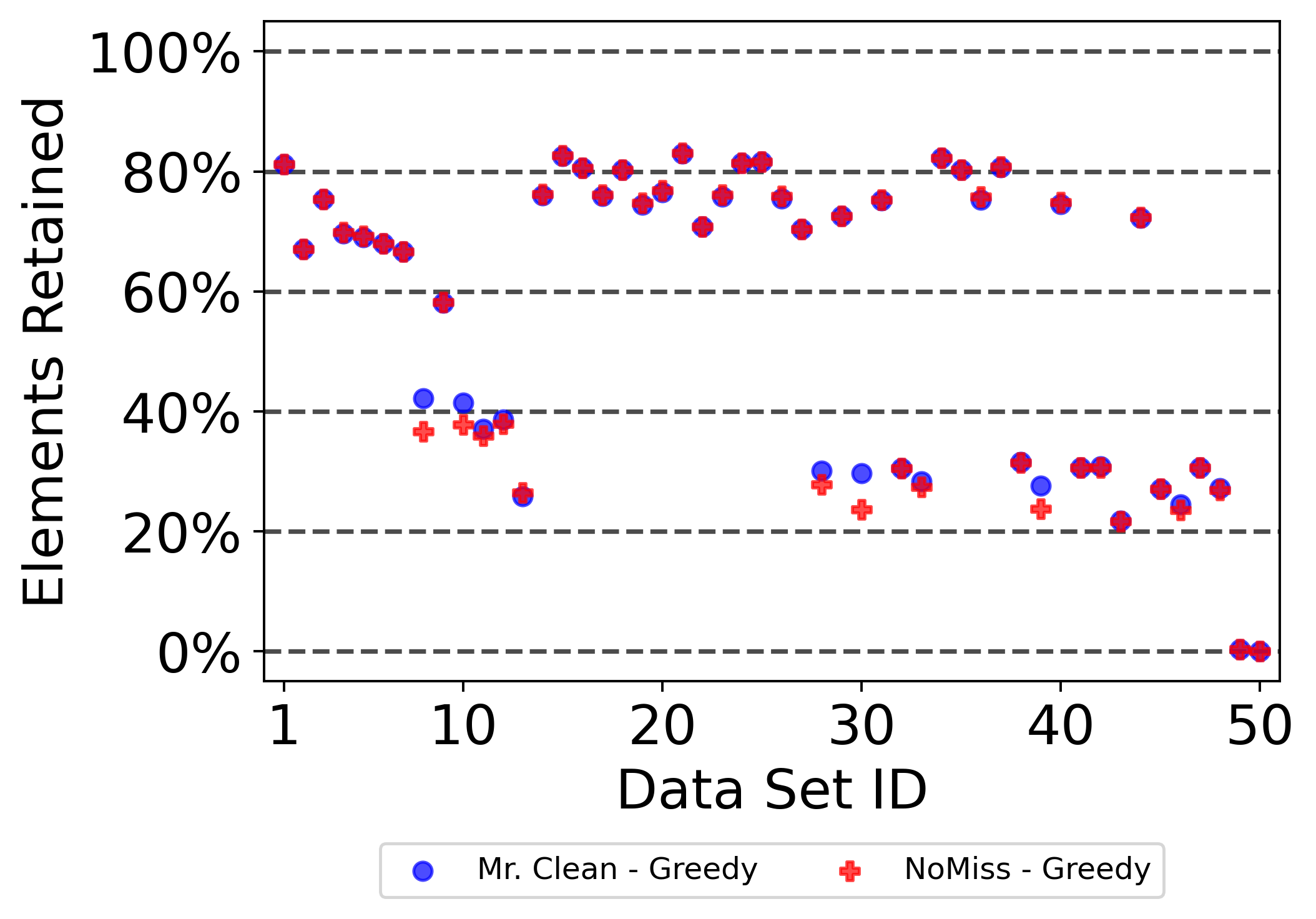
(a)

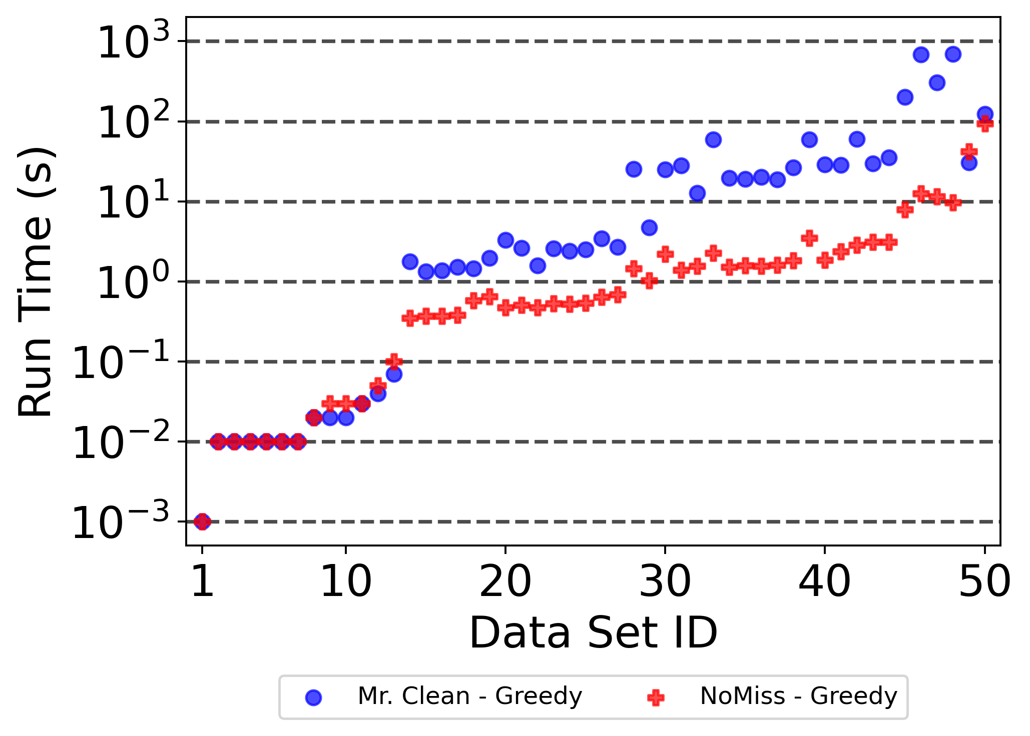
(b)

(c)

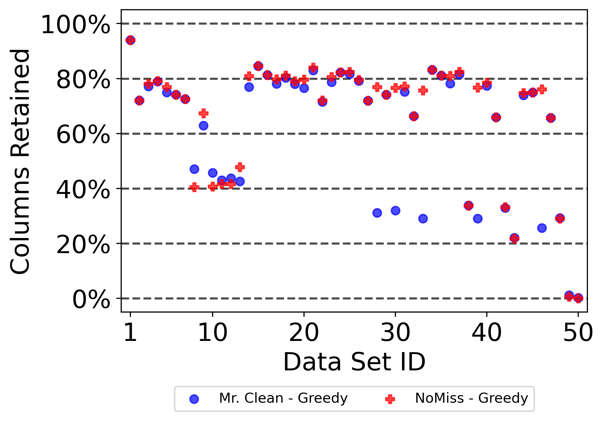
(d)

Figure 1: Comparison of Mr. Clean and NoMiss Greedy Algorithms. (a) Percentage of Original Valid Elements Retained (b) Run Time. (c) Percentage of Original Rows Retained. (d) Percent of Original Columns Retained.

The NoMiss - Greedy algorithm was substantially faster than Mr. Clean - Greedy in 35 of the 50 runs, as seen in Figure 1b. Both algorithms had the same run time (to within 0.001 seconds) for the first eight trials. However, Mr. Clean - Greedy quickly took an order of magnitude, or more, longer to run than NoMiss - Greedy. Luckily, the absolute run time of both algorithms was very quick, with the longest combined run time of $\sim 11.5$ minutes, occurring at data sets 46 and 48. Since the No Miss implementation had a quick run time, we decided to run both greedy algorithms when $\gamma=0$ and take the best solution. This approach is used in the rest of this manuscript.

In Figures 1c and 1d, we compared the percent of rows and columns retained by the two algorithms. The two algorithms retained the same number of rows in 19 data sets, but the same number of columns in only 12. These 12 instances were the only ones where the two algorithms returned a matrix with the same number of valid elements. In general, NoMiss - Greedy removed more rows and kept more columns. This is especially evident in a few instances near trials 30 and 40, where NoMiss - Greedy kept $\sim 30\%$ of the rows and $\sim 75\%$ of the columns, while Mr. Clean - Greedy kept $\sim 95\%$ of the rows and $\sim 30\%$ of the columns.

IV-B RowCol IP vs. RowCol LP

In Figure 2, we compare run time of both RowCol algorithms. On data sets 49 and 50, the RowCol IP timed out and the RowCol LP ran out of memory before solving. Overall, a major decrease in rum time (1-2 orders of magnitude) was achieved by the RowCol LP, which as able to solve data sets 1-48 in under 2100 seconds each, with most problems solving in under 1 second. When both algorithms converged, they returned a matrix with the same dimension. Due to its ability to converge quicker and on a wider range of data sets, the RowCol LP was selected for comparison to other programs in the $\gamma=0.0$ scenarios.

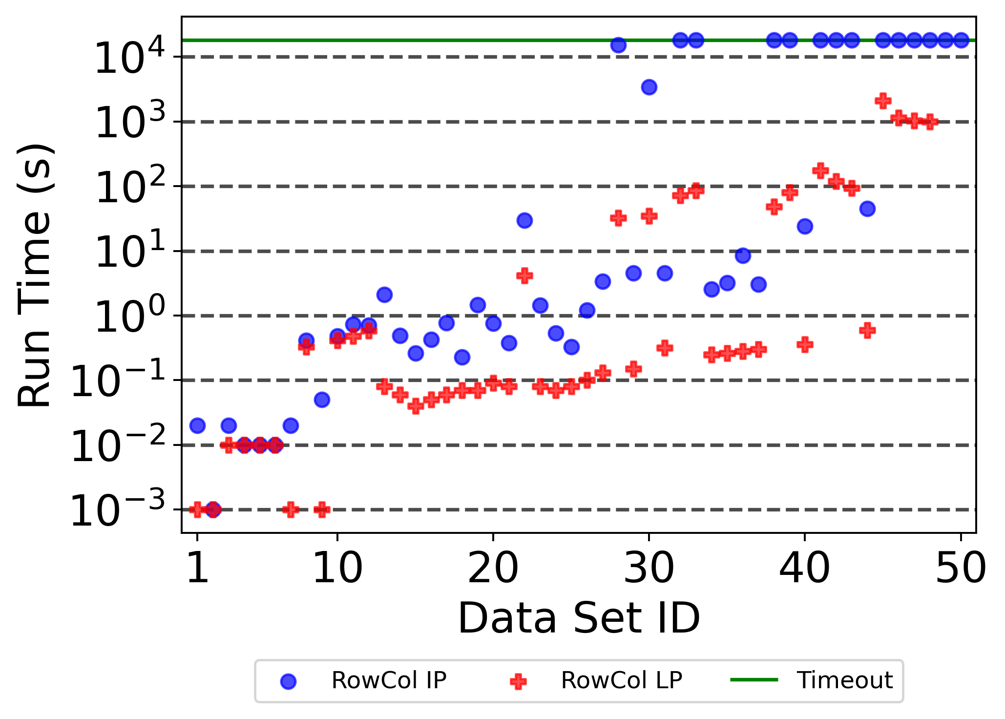
Figure 2: Run Time of RowCol IP and RowCol LP. The green line indicates the maximum allowed run time of 18000 seconds.

IV-C MaxCol IP vs. Element IP

Next we compare the run times of MaxCol MIP and Element IP in Figure 3. The MaxCol MIP was able to solve majority of the data sets within 10 seconds. However, data sets 13, 49, and 50 exhausted the available memory of the program, while MaxCol MIP timed out on data set 43. On the other hand, Element IP timed out for the majority of the data sets, only converging to a solution on data sets 1-12, and 14. Due to its reduced run time and its ability to converge for substantially more data sets, the MaxCol IP was selected to run in the $\gamma=0.0$ scenarios.

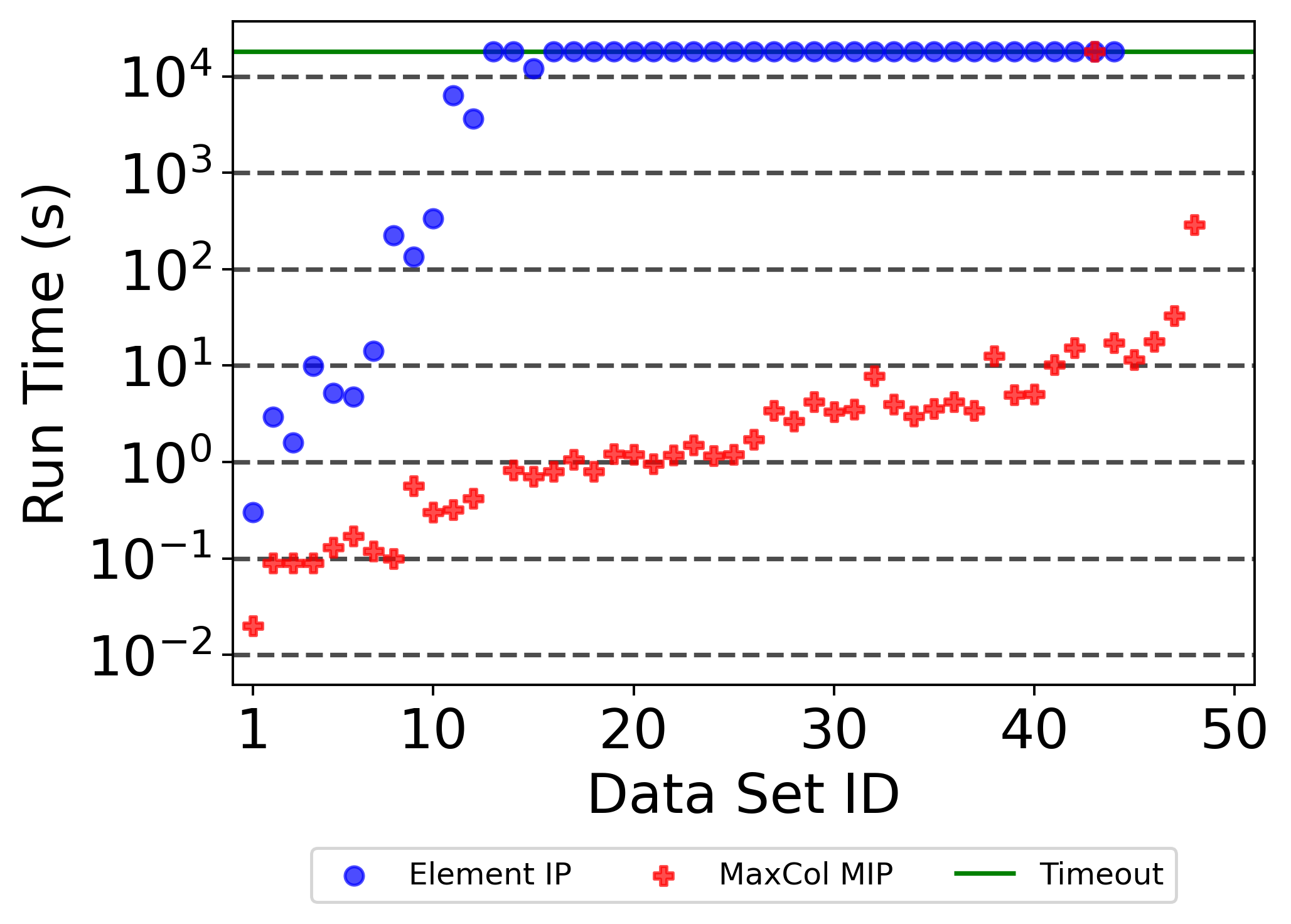
Figure 3: Run Time of MaxCol MIP and Element IP. The green line indicates the maximum allowed run time of 18000 seconds.

IV-D Comparing to Other Deletion Algorithms

In this section, we evaluate the NoMiss and Mr. Clean algorithms against existing data cleaning routines. Each of the 50 data sets were cleaned to 3 different maximum missingness values: $\gamma=0.0$, $\gamma=0.05$, and $\gamma=0.1$.

In the $\gamma=0.0$ scenario, we compared the combined greedy algorithm, RowCol LP, MaxCol MIP, list-wise, feature-wise, auto-miss, and DataRetainer programs, as seen in Figure 4. Figure 4a shows the percentage of original valid element retained by each algorithm. When MaxCol MIP solved the problem (data sets 1-12, 14-42, and 44-48), it achieved the most valid elements, as expected. Although, multiple algorithms often kept the maximum number of elements. For the remaining data sets, the maximum number of elements was obtained by greedy in 3 scenarios and DataRetainer in 1 scenario. The combined greedy algorithm kept the maximum number of elements in 36 scenarios, 33 of which were proven optimal. All of the additional scenarios were within 0.5% of maximum. The RowCol LP performed slightly worse, keeping the optimal number of elements in only 15 of the 48 scenarios, while failing to converge for data sets 49 and 50. Of the sub-optimal solutions, all were withing 0.5% of maximum, except for data set 13 which was $\sim$ 2.5% from optimal. The DataRetainer algorithms was the next most consistent, keeping the maximum number of elements in 15 scenarios. The Auto-miss program never retained the maximum number of elements, removing more than 95% of the possible elements in 38 scenarios. Since each row and/or column contained some missing data in several data sets, the list-wise algorithm performed the worse overall, removing all elements in 36 scenarios. The feature-wise algorithm removed all elements in 18 scenarios, but then performed well in 15 other scenarios, staying within 1% of optimal.

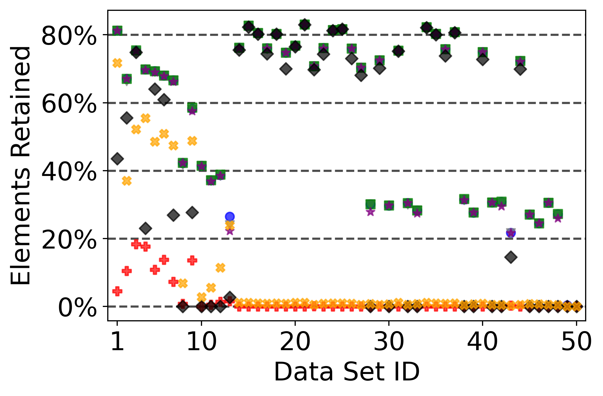
(a)

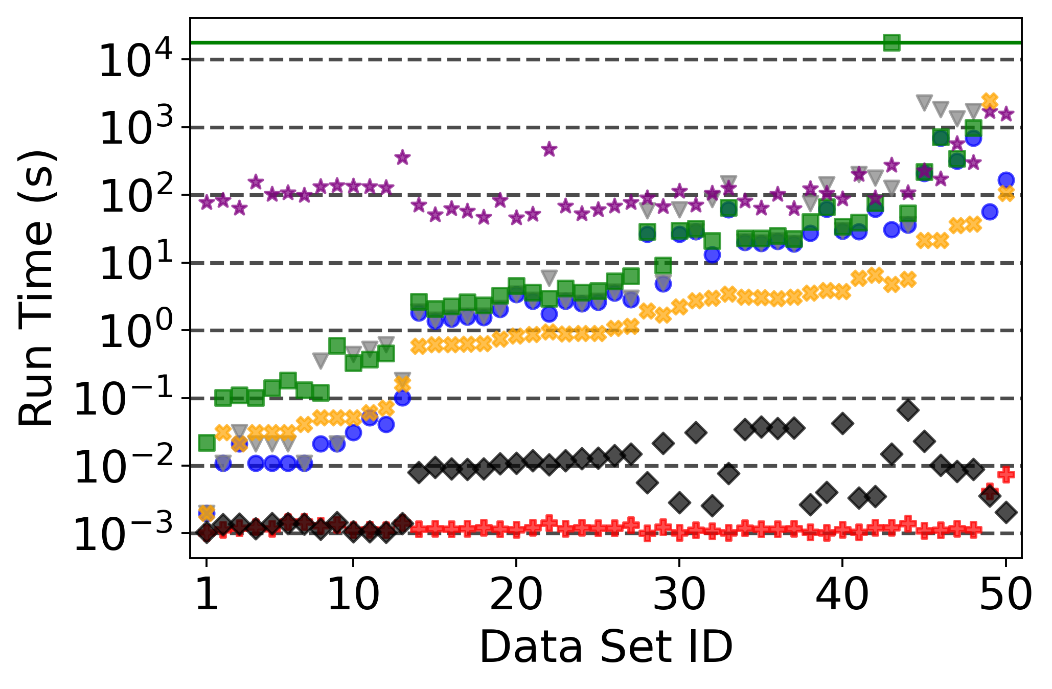
(b)

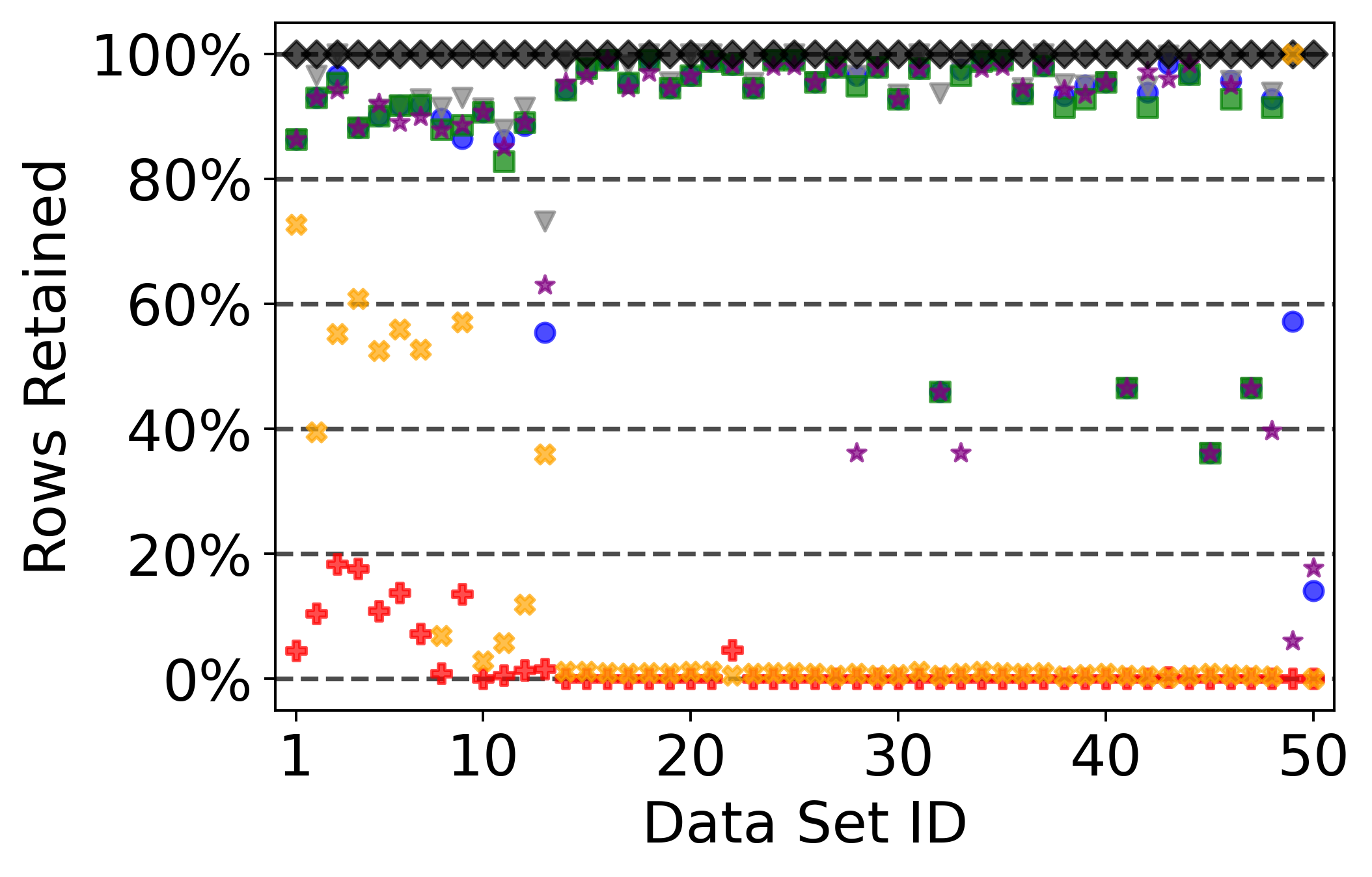
(c)

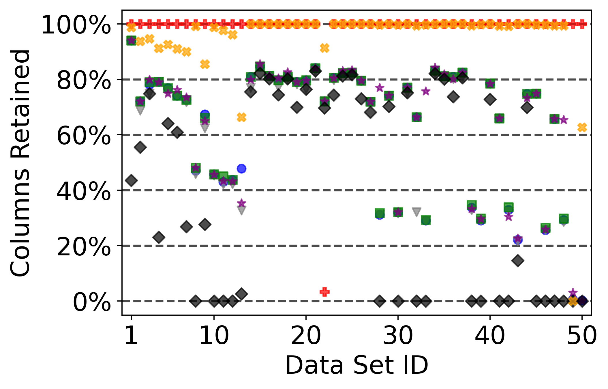
(d)

(e)

Figure 4: Comparison of Deletion Algorithms at $\gamma=0.0$. (a) Percentage of Original Valid Elements Retained (b) Run Time. (c) Percentage of Original Rows Retained. (d) Percent of Original Columns Retained.

DataRetainer dominated the run time for the first 40 scenarios and then gave way to the MaxCol MIP and RowCol LP, as shown in Figure 4b. In 27 scenarios, MaxCol MIP ran in under 10 seconds. In fact, MaxCol IP, RowCol LP, and the combined greedy ran at similar speeds for the first 27 scenarios. In Figure 4c we can see that list-wise and auto-miss removed the majority of the rows starting at data set 14. Similarly, feature-wise deleted the most columns as seen in Figure 4d. In some scenarios, DataRetainer created matrices much different than the NoMiss algorithms. While keeping the number of elements within 1% of optimal, the DataRetainer solution to data set 33 contained 1/3 the rows and 2.6 times the number of columns as the greedy solution. This demonstrates that dramatically different solutions can have similar objective values.

In the $\gamma=0.05$ and $\gamma=0.1$ scenarios, we compared the Mr. Clean algorithms to naive deletion and DataRetainer. The naive approach removes any row or column that exceeds the maximum percentage of missing data. Figure 5 shows the results of the programs at $\gamma=0.05$. The Element IP produced no solution for 16 data sets, 10 due to timeout and 6 due to memory limits. The remaining experiments were solved optimally. While the larger sets tended to be most difficult, data set 13 also plagued the program. The RowCol IP optimally solved 41 of the data sets and produced no solution for 8 data sets. The only set which RowCol IP solved sub-optimally was data set 10, in which it was within 0.002% of optimal. Mr. Clean greedy was able to clean all data sets, keeping the maximum number of valid elements in 42 sets and staying within 1% of the maximum kept in the rest. These sub-optimal solutions tended to occur within the smaller data sets. DataRetainer performed slightly worse, identifying the best solutions in 34 data sets. The sub-optimal solutions were also worse than Mr. Clean greedy, missing over 2% of the elements in three of the experiments. As expected, the naive approach removed the most elements. In some cases no valid elements were kept. This occurred when all of the rows, or all of the columns, contained more than 5% missing data.

The run times for $\gamma=0.05$ are compared in Figure 5b. Element IP and RowCol IP timed out on 9 data sets and 10 data sets, respectively, while solving the majority of the small and medium size data sets in under 60 seconds. All data sets were cleaned by Mr. Clean greedy in under 13 minutes, with most taking less than 1 minute. DataRetainer fell in between the IPs and greedy in terms of run time. Most data sets were cleaned within a minute, but the largest set took almost 27 minutes to clean. The naive approach processed all of the files the quickest. Most data sets took less than 0.5 seconds, with the longest run time of 6 seconds occurring for the largest data set.

The DataRetainer and Mr. clean algorithms produced solutions with similar dimensions for majority of data sets. Notable exceptions are trails 28, 33, 48, and 49. Some of these differences resulted in $\sim 5.5\%$ fewer elements (data set 28), while others resulted in only a small difference in elements ($1.1\%$ for data set 48). Instances of vastly different dimensions with a similar number of valid elements highlight the diversity of near optimal solutions.

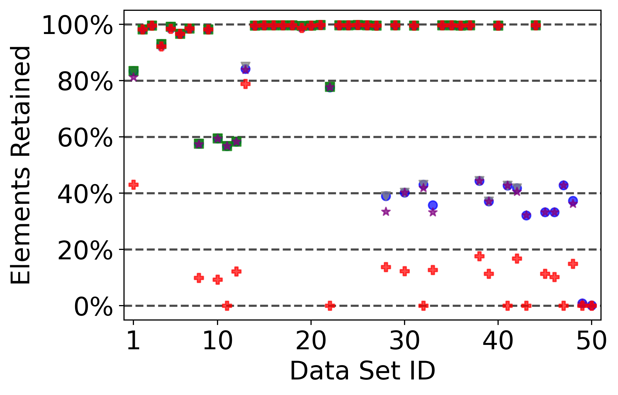
(a)

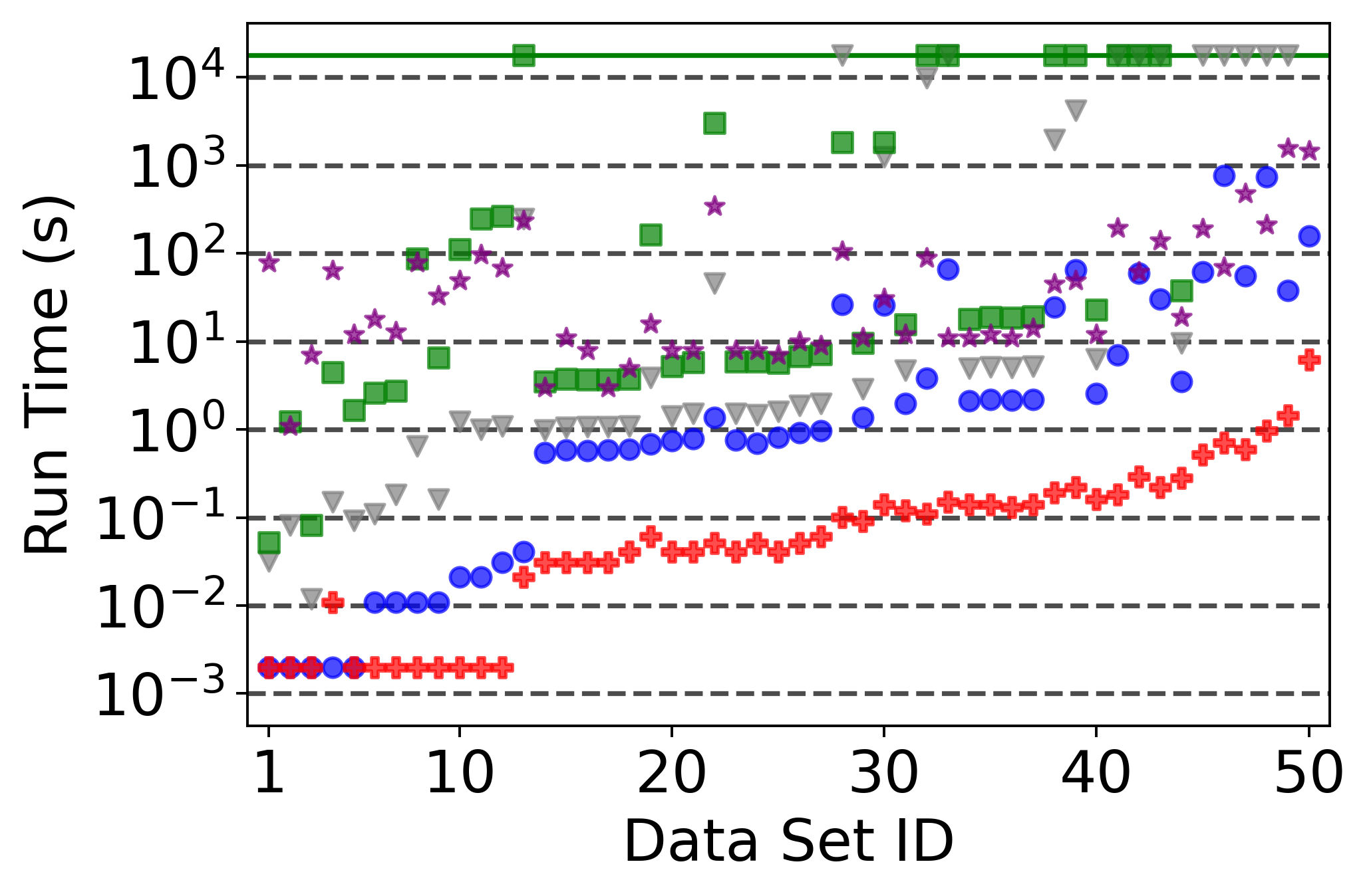
(b)

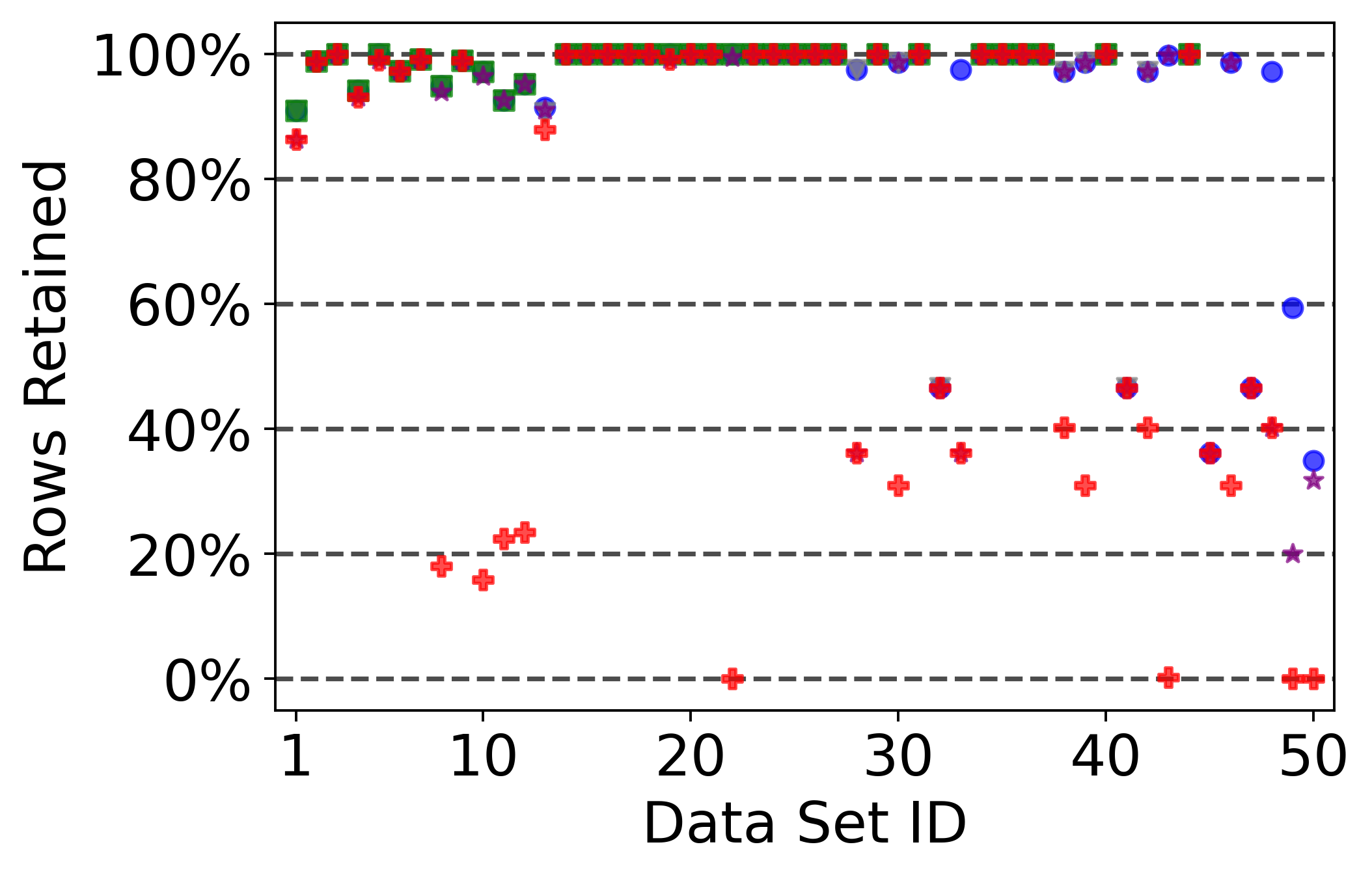
(c)

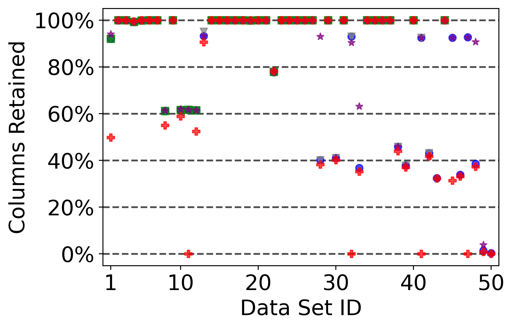
(d)

(e)

Figure 5: Comparison of Deletion Algorithms at $\gamma=0.05$. (a) Percentage of Original Valid Elements Retained (b) Run Time. (c) Percentage of Original Rows Retained. (d) Percent of Original Columns Retained.

Figure 6 shows the comparison between the deletion algorithms at $\gamma=0.1$. Element IP solved 35 data sets optimally and returned no solution for the remaining 15. All of these data sets were difficult for the program at $\gamma=0.05$ as well. RowCol IP failed to find a solution in 7 experiments, but retained the maximum number of elements in 42 experiments, 36 of which were proven optimal. Data set 33 proved the most difficult for RowCol IP, where it kept 1% fewer elements than greedy. The Mr. Clean greedy algorithm performed well again, retaining the most elements in 48 experiments. In the two cases where it failed to fine the best solution, it was still within 0.1%. DataRetainer performed slightly worse than greedy, retaining the maximum number of elements in 43 experiments. However, in 3 of the experiments, DataRetainer deleted over 1% more elements than required. The naive approach performed really well on some data sets, and then terribly on others.

The run times for $\gamma=0.1$ is shown in Figure 6b. The Element IP and DataRetainer alternate longest run time. Towards the middle of the graph (data sets 14-31) most data sets contained less than 10% missing data in each row and column. The run time for these experiments shows the difference in set-up and constraint checking time for the various methods. The RowCol IP and greedy algorithms show a similar run time pattern for many experiments, with the exception of the time out and near timeout runs. The solution dimensions between 4 of the algorithms were very consistent, as seen in Figures 6c and 6d. Decreases in the number of elements retained by the naive algorithm are matched by decreases in either Figure 6c or 6d. Similar to other experiments, there were a few data sets where DataRetainer found dramatically different solutions with a similar number valid elements compared to the Mr. Clean algorithms.

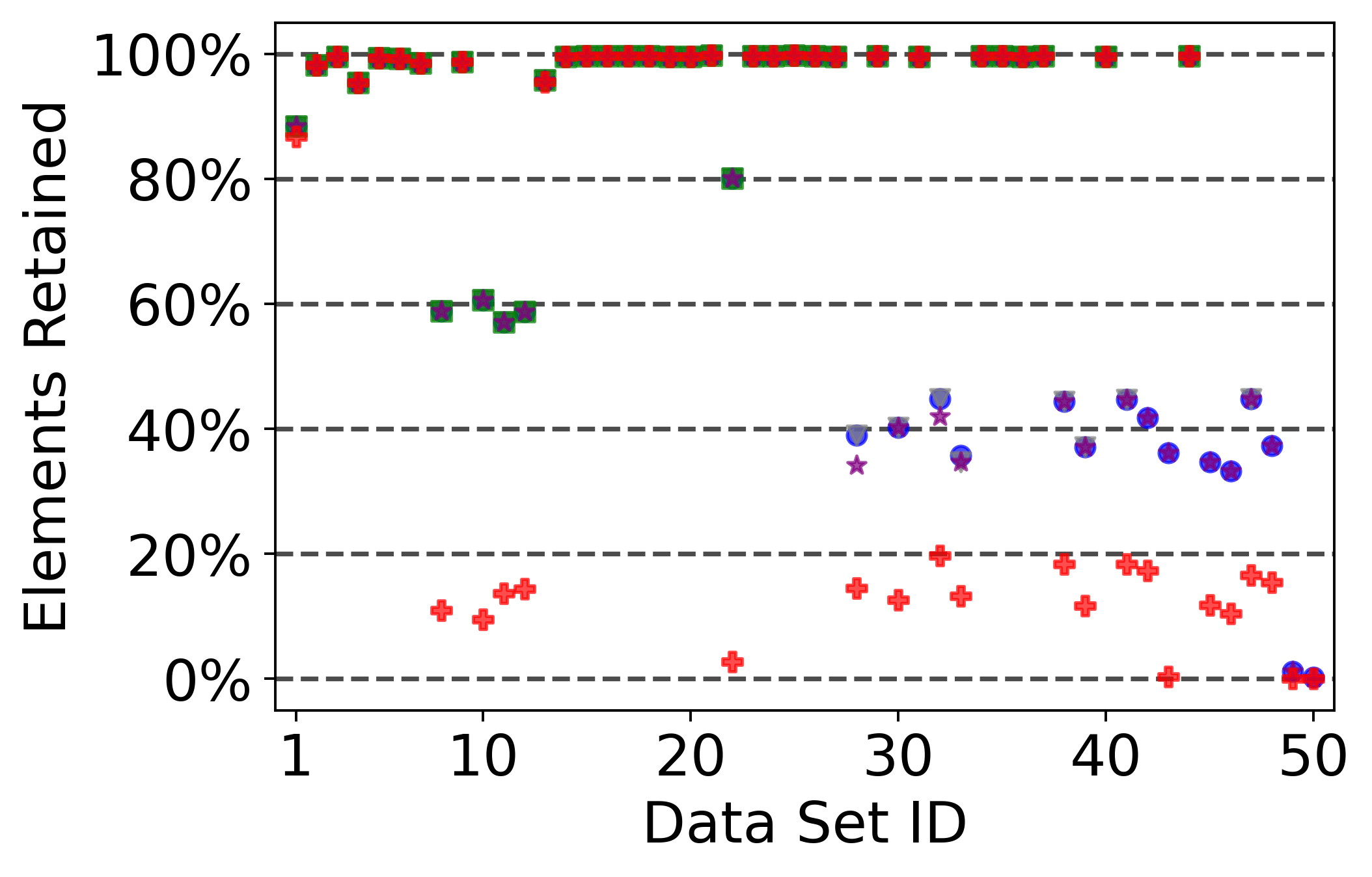
(a)

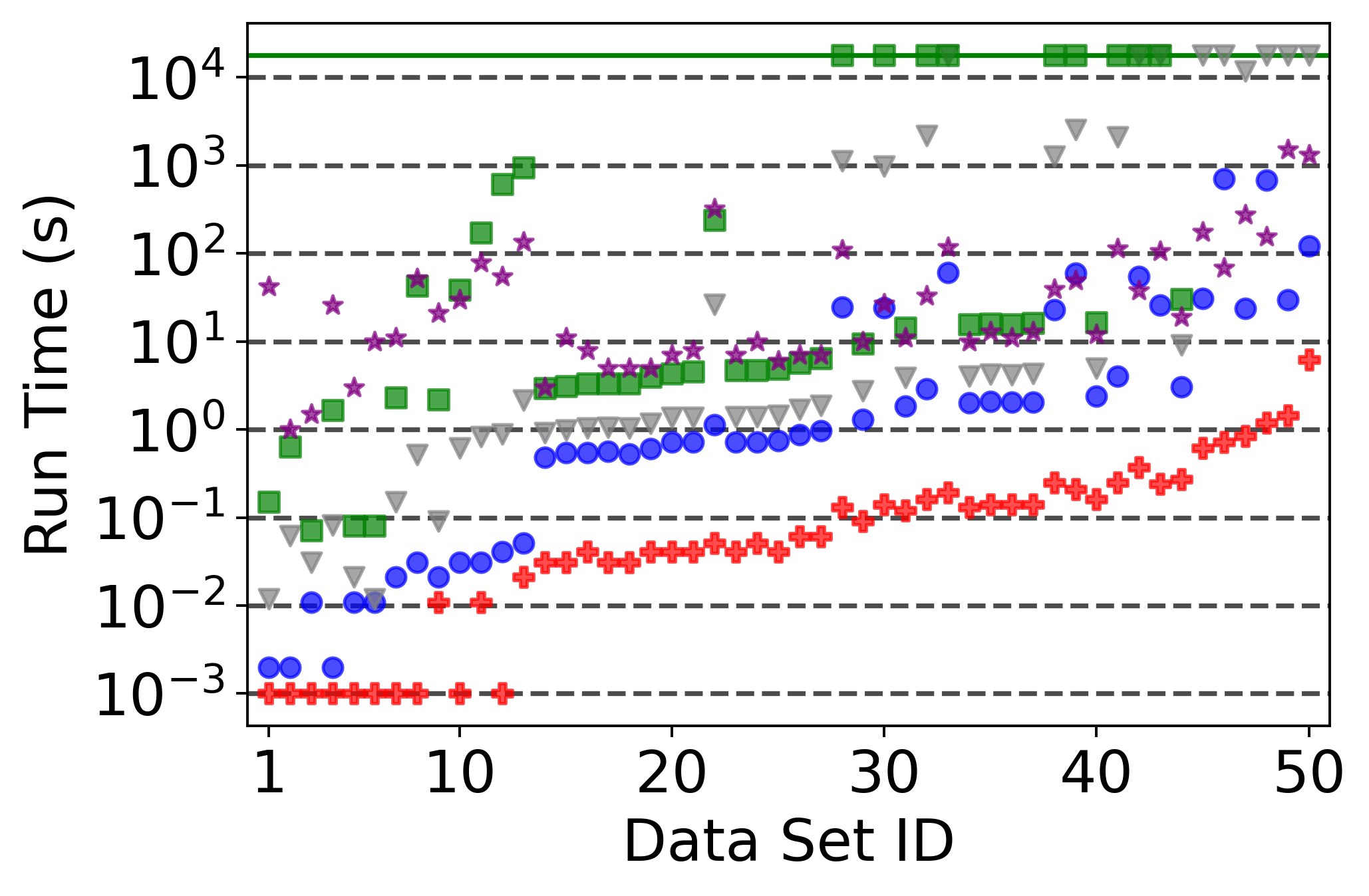
(b)

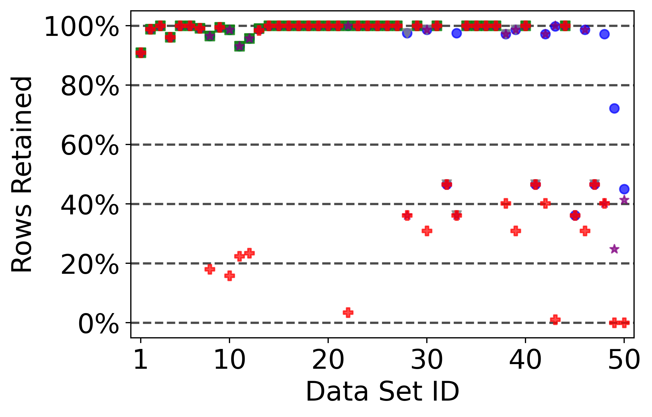
(c)

(d)

(e)

Figure 6: Comparison of Deletion Algorithms at $\gamma=0.1$. (a) Percentage of Original Valid Elements Retained (b) Run Time. (c) Percentage of Original Rows Retained. (d) Percent of Original Columns Retained.

V Conclusion

In this manuscript we recast the Mr. Clean IPs for the $\gamma=0.0$ scenario. We showed that the RowCol IP can be solved as a LP, reducing runtime and increasing the file size that could be processed. For the Element IP, we demonstrated that by partitioning the solution space and solving several simple MIPs in parallel, the run time could be dramatically reduced while increasing the maximum problem size. Finally, we added a new NoMiss greedy algorithm, which supplements the Mr. Clean greedy algorithm.

After comparing the NoMiss programs to their Mr. Clean counterparts, we evaluated both sets of programs against existing deletion algorithms. The new combined greedy algorithm proved to be the best balance between run time and retaining elements over all experiments. It was able to solve all problems and retained the most elements in 127 of 150 scenarios. The $\gamma=0.0$ experiments gave the algorithm the most difficulty. However, many of these experiments were optimally solved by the MaxCol MIP, which ran sufficiently fast to use in place of greedy when $\gamma=0.0$. This MIP handled all but 4 of data files in our 5 hour limit, with most solving within 10 seconds. The RowCol algorithms showed a slight improvement over greedy in a few scenarios, but only in ones that were successfully cleaned by Element IP. The list-wise, feature-wise, naive, and auto-miss algorithms while running very fast, removed considerably more elements than other approaches. The DataRetainer performed well on most of the scenarios, but required constant user interaction for each data set. We therefore recommend using the MaxCol MIP when cleaning data for $\gamma=0.0$ and utilizing the combined greedy algorithm for other $\gamma$ value, or if the data set is too large for the MaxCol MIP. Finally, the Element IP can be employed on small or medium data sets when extra runtime and memory are available.

Possible future work in this area could include creating a distributed version of Element IP for $\gamma>0.0$ scenarios or rerunning the IP/MIPs while controlling the minimum number of remaining rows and columns. It is also worth investigating the downstream impacts of partial deletion to imputation, along with better understanding the vast differences in matrix dimensions for near optimal solutions.

References

- [1] Akanksha Farswan, Anubha Gupta, Ritu Gupta and Gurvinder Kaur “Imputation of Gene Expression Data in Blood Cancer and Its Significance in Inferring Biological Pathways” In Frontiers in Oncology 9 Frontiers Media S.A., 2020 DOI: 10.3389/fonc.2019.01442
- [2] Aditya Dubey and Akhtar Rasool “Efficient technique of microarray missing data imputation using clustering and weighted nearest neighbour” In Scientific Reports 11 Nature Research, 2021 DOI: 10.1038/s41598-021-03438-x
- [3] Marcilio C.P.D. Souto, Pablo A. Jaskowiak and Ivan G. Costa “Impact of missing data imputation methods on gene expression clustering and classification” In BMC Bioinformatics 16 BioMed Central Ltd., 2015 DOI: 10.1186/s12859-015-0494-3
- [4] Margot Peeters, Mariëlle Zondervan-Zwijnenburg, Gerko Vink and Rens Schoot “How to handle missing data: A comparison of different approaches” In European Journal of Developmental Psychology 12 Psychology Press Ltd, 2015, pp. 377–394 DOI: 10.1080/17405629.2015.1049526
- [5] Paul Madley-Dowd, Rachael Hughes, Kate Tilling and Jon Heron “The proportion of missing data should not be used to guide decisions on multiple imputation” In Journal of Clinical Epidemiology 110 Elsevier USA, 2019, pp. 63–73 DOI: 10.1016/j.jclinepi.2019.02.016
- [6] Ben Omega Petrazzini et al. “Evaluation of different approaches for missing data imputation on features associated to genomic data” In BioData Mining 14 BioMed Central Ltd, 2021 DOI: 10.1186/s13040-021-00274-7
- [7] Donald B. Rubin “INFERENCE AND MISSING DATA” In ETS Research Bulletin Series 1975 John Wiley & Sons, Ltd, 1975, pp. i–19 DOI: 10.1002/J.2333-8504.1975.TB01053.X
- [8] Andrew Briggs, Clark Taane, Jane Wolstenholme and Philip Clarke “Missing…. presumed at random: cost-analysis of incomplete data” In Health Econcomics 12, 2003, pp. 377–392 DOI: 10.1002/hec.766
- [9] Daniel A. Newman “Missing Data: Five Practical Guidelines” In Organizational Research Methods 17 SAGE Publications Inc., 2014, pp. 372–411 DOI: 10.1177/1094428114548590
- [10] Joost R. Ginkel, Marielle Linting, Ralph C.A. Rippe and Anja Voort “Rebutting Existing Misconceptions About Multiple Imputation as a Method for Handling Missing Data” In Journal of Personality Assessment 102 Routledge, 2020, pp. 297–308 DOI: 10.1080/00223891.2018.1530680
- [11] Sharlee Climer, Alan R. Templeton and Weixiong Zhang “Allele-Specific Network Reveals Combinatorial Interaction That Transcends Small Effects in Psoriasis GWAS” In PLoS Computational Biology 10, 2014 DOI: 10.1371/journal.pcbi.1003766
- [12] Sharlee Climer “Connecting the dots: The boons and banes of network modeling” In Patterns 2 Cell Press, 2021 DOI: 10.1016/j.patter.2021.100374
- [13] Michael Chan “auto-miss” GitHub, 2019 URL: https://github.com/ClimerLab/auto-miss.
- [14] Kenneth Smith and Sharlee Climer “Mr. Clean: An Ensemble of Data Cleaning Algorithms for Increased Data Retention”
- [15] Hyunsoo Kim, Gene H. Golub and Haesun Park “Missing value estimation for DNA microarray gene expression data: local least squares imputation” In Bioinformatics 21, 2005, pp. 187–198 DOI: 10.1093/bioinformatics/bth499
- [16] Olga Troyanskaya et al. “Missing value estimation methods for DNA microarrays” In Bioinformatics 17, 2001, pp. 520–525 DOI: 10.1093/bioinformatics/17.6.520
- [17] Shigeyuki Oba et al. “A Bayesian missing value estimation method for gene expression profile data” In Bioinformatics 19, 2003, pp. 2088–2096 DOI: 10.1093/bioinformatics/btg287
- [18] T.. Bo “LSimpute: accurate estimation of missing values in microarray data with least squares methods” In Nucleic Acids Research 32, 2004, pp. 34e–34 DOI: 10.1093/nar/gnh026
- [19] Wei-Chao Lin and Chih-Fong Tsai “Missing value imputation: a review and analysis of the literature (2006–2017)” In Artificial Intelligence Review 53, 2020, pp. 1487–1509 DOI: 10.1007/s10462-019-09709-4
- [20] Carol M. Musil, Camille B. Warner, Piyanee Klainin Yobas and Susan L. Jones “A Comparison of Imputation Techniques for Handling Missing Data” In Western Journal of Nursing Research 24, 2002, pp. 815–829 DOI: 10.1177/019394502762477004
- [21] Peter C. Austin, Ian R. White, Douglas S. Lee and Stef Buuren “Missing Data in Clinical Research: A Tutorial on Multiple Imputation” In Canadian Journal of Cardiology 37 Elsevier Inc., 2021, pp. 1322–1331 DOI: 10.1016/j.cjca.2020.11.010
- [22] Adrienne D Woods et al. “Missing Data and Multiple Imputation Decision Tree” In PsyArXiv, 2021 DOI: 10.31234/osf.io/mdw5r
- [23] Jungyeon Choi, Olaf M. Dekkers and Saskia Cessie “A comparison of different methods to handle missing data in the context of propensity score analysis” In European Journal of Epidemiology 34 Springer Netherlands, 2019, pp. 23–36 DOI: 10.1007/s10654-018-0447-z
- [24] Thomas L. Saaty “Optimization in Integers and Related Extremal Problems.” McGraw-Hill, Inc, 1970, pp. 1–295 DOI: 10.2307/2316512
- [25] Kelly A. Frazer et al. “A second generation human haplotype map of over 3.1 million SNPs” In Nature 449, 2007, pp. 851–861 DOI: 10.1038/nature06258
- [26] Kevin Dunn “Kamyr digester-OpenMV.net Datasets.” In OpenMV.net, 2011 URL: https://openmv.net/info/kamyr-digester
- [27] Bhupinder S Dayal et al. “Application of feedforward: neural networks and partial least squares regression for modelling kappa number in a continuous Kamyr digester: how multivariate data analysis might help pulping”, 1994
- [28] Bingshan Li et al. “Transcriptome analysis of psoriasis in a large case-control sample: RNA-seq provides insights into disease mechanisms” In Journal of Investigative Dermatology 134 Elsevier Masson SAS, 2014, pp. 1828–1838 DOI: 10.1038/jid.2014.28
- [29] Peter M Szabo et al. “Cancer-associated fibroblasts are the main contributors to epithelial-to-mesenchymal signatures in the tumor microenvironment” In Scientific Reports 13, 2023 DOI: 10.1038/s41598-023-28480-9
- [30] Chengran Yang et al. “Genomic atlas of the proteome from brain, CSF and plasma prioritizes proteins implicated in neurological disorders” In Nature Neuroscience 24, 2021, pp. 1302–1312 DOI: 10.1038/s41593-021-00886-6
- [31] Benjamin Izar et al. “A single-cell landscape of high-grade serous ovarian cancer” In Nature Medicine 26 Nature Research, 2020, pp. 1271–1279 DOI: 10.1038/s41591-020-0926-0
- [32] Jared Liu et al. “Single-cell RNA sequencing of psoriatic skin identifies pathogenic Tc17 cell subsets and reveals distinctions between CD8+ T cells in autoimmunity and cancer” In Journal of Allergy and Clinical Immunology 147 Mosby Inc., 2021, pp. 2370–2380 DOI: 10.1016/j.jaci.2020.11.028