Learning parameter dependence for Fourier-based option pricing with tensor networks

Abstract

A long-standing issue in mathematical finance is the speed-up of option pricing, especially for multi-asset options. A recent study has proposed to use tensor train learning algorithms to speed up Fourier transform (FT)-based option pricing, utilizing the ability of tensor networks to compress high-dimensional tensors. Another usage of the tensor network is to compress functions, including their parameter dependence. Here, we propose a pricing method, where, by a tensor learning algorithm, we build tensor trains that approximate functions appearing in FT-based option pricing with their parameter dependence and efficiently calculate the option price for the varying input parameters. As a benchmark test, we run the proposed method to price a multi-asset option for the various values of volatilities and present asset prices. We show that, in the tested cases involving up to 11 assets, the proposed method outperforms MC-based option pricing with $10^{5}$ paths in terms of computational complexity while keeping comparable accuracy.

 

Contents

1. 1 Introduction
2. 2 Tensor train
   1. 2.1 Compression tenchniques
      1. 2.1.1 Tensor cross interpolation
      2. 2.1.2 Singular value decomposition
3. 3 Fourier transform-based option pricing aided by tensor cross interpolation
   1. 3.1 Fourier transform-based option pricing
   2. 3.2 Fourier transform-based option pricing with tensor trains
   3. 3.3 Monte Carlo-based option pricing
4. 4 Learning parameter dependence with tensor networks
   1. 4.1 Outline
   2. 4.2 Computational complexity
5. 5 Numerical demonstration
   1. 5.1 Details
   2. 5.2 Results
      1. 5.2.1 The case of varying $\vec{\sigma}$
      2. 5.2.2 The case of varying $\vec{S_{0}}$
      3. 5.2.3 Randomness in learning the TTs
      4. 5.2.4 Total computational time for obtaining the MPOs
6. 6 Summary and discussion
7. A How to set the tolerance $\epsilon_{\mathrm{SVD}}$

 

1 Introduction

Financial firms are conducting demanding numerical calculations in their business. One of the most prominent ones is option pricing. An option is a financial contract in which one party, upon specific conditions being met, pays an amount (payoff) determined by the prices of underlying assets such as stocks and bonds to the other party. Concerning the time when the payoff occurs, the simplest and most common type of options is the European type, which this paper hereafter focuses on: at the predetermined future time (maturity) $T$, the payoff $v(\vec{S}(T))$ depending on the underlying asset prices $\vec{S}(T)$ at time $T$ occurs. For example, in a European call/put option, one party has the right to buy/sell an asset at the predetermined price (strike) $K$ and maturity $T$, and the corresponding payoff function is $v(S(T))=\max\{c(S(T)-K),0\}$, where $c=1$ and $-1$ for a call and put option, respectively. In addition to this simple one, various types of options are traded and constitute a large part of the financial industry.

Pricing options appropriately is needed for making a profit and managing the risk of loss in option trading. According to the theory in mathematical finance , the price of an option is given by the expectation of the discounted payoff in the contract with some stochastic model on the dynamics of underlying asset prices assumed. Except for limited cases with simple contract conditions and models, the analytical formula for the option price is not available and thus we need to resort to the numerical calculation. In the rapidly changing financial market, quick and accurate pricing is vital in option trading, but it is a challenging task, for which long-lasting research has been made. In particular, pricing multi-asset options, whose payoff depends on the prices of multiple underlying assets, is often demanding. Many pricing methodologies suffer from the so-called curse of dimensionality, which means the exponential increase of computational complexity with respect to the asset number, and the Monte Carlo method, which may evade the exponential complexity, has a slow convergence rate.

Motivated by these points, recently, applications of quantum computing to option pricing are considered actively. For example, many studies have focused on applications of the quantum algorithm for Monte Carlo integration [4], which provides the quadratic quantum speed-up over the classical counterpart. Unfortunately, running such a quantum algorithm requires fault-tolerant quantum computers, which may take decades to be developed.

In light of this, applications of quantum-inspired algorithms, that is tensor network (TN) algorithms, to option pricing have also been studied as solutions in the present or the near future [5, 6, 7, 8]. Among them, this paper focuses on the application of tensor train (TT) [9] learning to the Fourier transform (FT)-based option pricing method [10, 11], following the original proposal in [6]. This option pricing method is based on converting the integration for the expected payoff in the space of the asset prices $\vec{S}(T)$ to that in the Fourier space, namely, the space of $\vec{z}$, the wavenumbers corresponding to the logarithm of $\vec{S}(T)$. After this conversion, the numerical integration is done more efficiently in many cases. Unfortunately, as is common in numerical integration of multivariate functions, this approach suffers from the curse of dimensionality: the FT-based method is efficient for single-asset options but for multi-asset options, its computational complexity increases exponentially. On the other hand, tensor network is the technique originally developed in quantum many-body physics to express state vectors with exponentially large dimension efficiently and recently, it has also been utilized in various fields such as machine learning [14, 15], quantum field theory [16, 17, 18], and partial differential equations [7, 19]. Ref. [6] proposed to leverage the ability of tensor network to compress data as a high-dimensional tensor in order to express the functions of $\vec{z}$ involved in FT-based option pricing. The authors built TTs, a kind of tensor network, approximating those functions by a TT learning algorithm called tensor cross interpolation (TCI) [20, 21, 17, 22] and evaluated the integral involving them efficiently, which led to the significant speed-up of FT-based option pricing in their test cases.

Here, we would like to point out an issue in this TT-based method. That is, we need to rerun TCI to obtain TTs each time the parameters are changed. According to our numerical experiments, TCI takes a longer time than the Monte Carlo method, which means that the TT-based method does not have a computational time advantage.

To address this issue, we focus on another usage of tensor networks that can embed parameter dependence [23, 24, 25] to make FT-based option pricing more efficient. Namely, we learn TTs that approximate the functions including not only the dependence on $\vec{z}$ but also that on parameters in the asset price model such as the volatilities and the present asset prices, by a single application of TCI for each function. We use these tensor networks to perform fast option pricing in response to various parameter changes. To evaluate this approach, we consider two scenarios as benchmarks, varying volatilities and present stock prices. In the test cases, it is seen that for up to 11 assets, the computational complexity of our proposed method, which is measured by the number of elementary operations is advantageous to that of the Monte Carlo method with $10^{5}$ paths, a common setting in practice. Indeed, the computational complexity of our proposed method is better than that of Monte Carlo by a factor of $O(10^{4})$ for $d<10$ and by a factor of $O(10^{3})$ for about $d=10$ or $11$ (refer to FIG. 2). We also confirm numerically that the accuracy of our method is within the statistical error in the Monte Carlo method with $10^{5}$ paths. In summary, these results suggest that at least in some cases, our proposed method has advantages over Monte Carlo in terms of computational complexity, keeping the accuracy.

The rest of this paper is organized as follows. Sec. II is devoted to introducing the tensor train and tensor learning algorithm. In Sec. III, we review the FT-based option pricing and its reformulation aided by TCI. We propose a new scheme for fast option pricing by learning tensor networks with parameter dependence in Sec. IV. We show the results of the numerical demonstration of our method applied to a kind of multi-asset option for the various values of the volatilities and the present asset prices in Sec. V. The summary and discussions are given in Sec. VI.

2 Tensor train

A $d$-way tensor $F_{x_{1},\dots,x_{d}}$, where each local index $x_{l}$, $l=1,\dots,d$, has a local dimension $N$, can be decomposed into a TT format with a low-rank structure. The TT decomposition of $F_{x_{1},\ldots,x_{d}}$ can be expressed as follows.

$$F_{x_{1},\ldots,x_{d}} \approx\sum_{l_{1}}^{\chi_{1}}\cdots\sum_{l_{d-1}}^{\chi_{d}}F_{l_{1},x_{1}}^{(1)}F_{l_{1}l_{2},x_{2}}^{(2)}\cdots F_{l_{d-1},x_{d}}^{(d)}$$

$$\equiv F_{x_{1}}^{(1)}\cdot F_{x_{2}}^{(2)}\cdot(\cdots)\cdot F_{x_{d}}^{(d)}$$ (1)

where $F_{x_{i}}^{(i)}$ denotes each 3-way tensor, $l_{i}$ represents the virtual bond index, and $\chi_{i}$ is the dimension of the virtual bond. One of the main advantages of TT is that it significantly reduces computational complexity and memory requirements by reducing bond dimensions $\chi_{i}$.

This is an equivalent expression to the wave function $F_{x_{1},\ldots,x_{d}}$ of a quantum system with $d$ $N$-level qudits as follows:

$$\ket{F_{x_{1},x_{2},\ldots,x_{d}}}=\sum_{l_{1}}^{\chi_{1}}\cdots\sum_{l_{d-1}}^{\chi_{d}}F_{l_{1},x_{1}}^{(1)}F_{l_{1}l_{2},x_{2}}^{(2)}\cdots F_{l_{d-1},x_{d}}^{(d)}\ket{\vec{x}},$$ (2)

where $\ket{\vec{x}}=\ket{x_{1}}\cdots\ket{x_{d}}$ is the tensor product of $\ket{x_{1}},\cdots,\ket{x_{d}}$, the basis states from $\ket{1}$ to $\ket{N}$.

2.1 Compression tenchniques

We introduce the two compression techniques used in this study.

2.1.1 Tensor cross interpolation

Tensor cross interpolation (TCI) is a technique to compress tensors corresponding to discretized multivariate functions with a low-rank TT representation. Here, we consider a tensor that, with grid points set in $\mathbb{R}^{d}$, has entries $F_{x_{1},\ldots,x_{d}}$ equal to $F(x_{1},\ldots,x_{d})$, the values of a function $F$ on the grid points. Leaving the detailed explanation to Refs. [20, 21, 17, 22], we describe its outline. It learns a TT using the values of the target function $F_{x_{1},x_{2}\ldots,x_{d}}$ at indexes $(x_{1},x_{2},\cdots,x_{d})$ adaptively sampled according to the specific rules. TCI actively inserts adaptively chosen interpolation points (pivots) from the sample points to learn the TT, which can be seen as a type of active learning. It gives the estimated values of the function at points across the entire domain although we use only the function values at a small number of sample points in learning. This is the very advantage of TCI and is particularly useful for compressing target tensors with a vast number of elements, contrary to singular value decomposition (SVD) requiring access to the full tensor. Note that TCI is a heuristic method, which means its effectiveness heavily depends on the internal algorithm to choose the pivots and the initial set of points selected randomly.

In this study, when we learn TT from functions with TCI, we add the pivots so that the error in the maximum norm $(\epsilon_{\mathrm{TCI}})$ is to be minimized.

$$\epsilon_{\mathrm{max}}=\frac{\|F_{x_{1},x_{2},\ldots,x_{d}}-\tilde{F}_{\mathrm{TT}}\|_{\mathrm{max}}}{\|F_{x_{1},x_{2},\ldots,x_{d}}\|_{\mathrm{max}}}$$ (3)

where $F_{x_{1},x_{2},\ldots,x_{d}}$ is a target tensor, $\tilde{F}_{\mathrm{TT}}$ is a low-rank approximation, and the maximum norm is evaluated as the maximum of the absolute values of the entries at the pivots selected already. The computational complexity of TCI is roughly proportional to the number of elements in the TT, which is $O(d\chi^{2}N)$ with $\chi_{1},\cdots,\chi_{d}$ fixed to $\chi$. In addition, considering the case that zero is included in the reference function value, the error should be normalized by $\|F_{x_{1},x_{2},\ldots,x_{d}}\|_{\mathrm{max}}$.

2.1.2 Singular value decomposition

In this study, we use singular value decomposition (SVD) to compress further the TTs obtained by TCI with its error threshold $\epsilon_{\mathrm{TCI}}$ set to a sufficiently low. The TT obtained from TCI, denoted as $F_{\mathrm{TT}}$, can be approximated by another TT, $\tilde{F}_{\mathrm{TT}}$, with reduced (optimized) bond dimensions such that

$$\frac{\|F_{\mathrm{TT}}-\tilde{F}_{\mathrm{TT}}\|_{\mathrm{F}}^{2}}{\|F_{\mathrm{TT}}\|_{\mathrm{F}}^{2}}<\epsilon_{\mathrm{SVD}},$$ (4)

where $\|\cdots\|_{\mathrm{F}}$ denotes the Frobenius norm. Note that the approximation error is conventionally expressed as the squared deviation. Given a tolerance $\epsilon_{\mathrm{SVD}}$, truncation via SVD results in an optimally low-rank TT approximation characterized by the smallest possible rank. For more technical details, readers are referred to Ref. [26].

3 Fourier transform-based option pricing aided by tensor cross interpolation

3.1 Fourier transform-based option pricing

In this paper, we consider the underlying asset prices $\vec{S}(t)=(S_{1}(t),\cdots,S_{d}(t))$ in the Black-Scholes (BS) model described by the following stochastic differential equation

$$dS_{m}(t)=rS_{m}(t)dt+\sigma_{m}S_{m}(t)dW_{m}(t).$$ (5)

Here, $W_{1}(t),\cdots,W_{d}(t)$ are the Brownian motions with constant correlation matrix $\rho_{ij}$, namely

$$dW_{m}(t)dW_{n}(t)=\rho_{mn}dt,$$ (10)

where $r\in\mathbb{R}$ and $\sigma_{1},\cdots,\sigma_{d}>0$ are constant parameters called the risk-free interest rate and the volatilities, respectively. The present time is set to $t=0$ and the present asset prices are denoted by $\vec{S}_{0}=(S_{1,0},\cdots,S_{d,0})$.

We consider European-type options, in which the payoff $v(\vec{S}(T))$ depending on the asset prices $\vec{S}(T)$ at the maturity $T$ occurs at $T$. According to the theory of option pricing, the price $V$ of such an option is given by the expectation of the discounted payoff:

$$V(\vec{p}) =\mathbb{E}\left[e^{-rT}v(\vec{S}(T))\middle|\vec{S}_{0}\right]$$

$$=e^{-rT}\int_{-\infty}^{\infty}v(\exp(\vec{x}))q(\vec{x}|\vec{x}_{0})dx,$$ (6)

where we define $\exp(\vec{x}):=(e^{x_{1}},\cdots,e^{x_{d}})$. $q(\vec{x}|\vec{x}_{0})$ is the probability density function of $\vec{x}:=(\log S_{1}(T),\cdots,\log S_{d}(T))$, the log asset prices at $T$, conditioned on the present value $\vec{x}_{0}=(\log S_{1,0},\cdots,\log S_{d,0})$. In the BS model defined by (5), $q(\vec{x}|\vec{x}_{0})$ is given by the $d$-variate normal distribution:

$$q(\vec{x}|\vec{x}_{0})=\frac{1}{\sqrt{(2\pi)^{d}\det\Sigma}}\exp\left(-\frac{1}{2}\left(\vec{x}-\vec{\mu}\right)^{T}\Sigma^{-1}\left(\vec{x}-\vec{\mu}\right)\right),$$ (7)

where $\Sigma:=(\sigma_{m}\sigma_{n}\rho_{mn}T)_{mn}$ is the covariance matrix of $\vec{x}$ and $\vec{\mu}:=\vec{x}_{0}+\left(rT-\frac{1}{2}\sigma_{1}^{2}T,\cdots,rT-\frac{1}{2}\sigma_{d}^{2}T\right)$. Note that, in Eq. (6), we denote the option price by $V(\vec{p})$, indicating its dependence on the parameter $\vec{p}$ such as the volatilities $\vec{\sigma}=(\sigma_{1},\cdots,\sigma_{d})$ and the present asset prices $\vec{S}_{0}$.

In FT-based option pricing, we rewrite the formula (6) as the integral in the Fourier space:

$$V(\vec{p})=\frac{e^{-rT}}{2\pi}\int_{\mathbb{R}^{d}+i\vec{\alpha}}\phi(-\vec{z})\hat{v}(\vec{z})d\vec{z}.$$ (8)

Here, $\vec{z}=(z_{1},\cdots,z_{d})$ is the wavenumber vector corresponding to $\vec{x}$.

$$\phi(\vec{z}):=\mathbb{E}[e^{i\vec{z}\cdot\vec{x}}|\vec{x}_{0}]=\int_{\mathbb{R}^{d}}e^{i\vec{z}\cdot\vec{x}}q(\vec{x}|\vec{x}_{0})d\vec{x}$$ (9)

is the characteristic function, and in the BS model, it is given by

$$\phi(\vec{z})=\exp\left(i\sum_{m=1}^{d}z_{m}\mu_{m}-\frac{T}{2}\sum_{m=1}^{d}\sum_{k=1}^{d}\sigma_{m}\sigma_{k}z_{m}z_{k}\rho_{mk}\right).$$ (10)

$\hat{v}(\vec{z}):=\int_{\mathbb{R}^{d}}e^{i\vec{z}\cdot\vec{x}}v(\exp(\vec{x}))d\vec{x}$ is the Fourier transform of the payoff function $v$, and its explicit formula is known for some types of options. For example, for a European min-call option with strike $K$, which we will consider in our numerical demonstration, the payoff function is

$$v_{\text{min}}(\vec{S}_{T})=\max\{\min\{S_{1}(T),\ldots,S_{d}(T)\}-K,0\}$$ (11)

and its Fourier transform is [27]

$$\hat{v}_{\min}(\vec{z})=-\frac{K^{1+i\sum_{m=1}^{d}z_{m}}}{(-1)^{d}\left(1+i\sum_{m=1}^{d}z_{m}\right)\prod_{m=1}^{d}(iz_{m})}.$$ (12)

Note that for $\hat{v}_{\min}(\vec{z})$ to be well defined, $\vec{z}\in\mathbb{C}^{d}$ must be taken so that $\imaginary z_{m}>0$ and $\sum_{m=1}^{d}\imaginary z_{m}>1$. $\vec{\alpha}\in\mathbb{R}^{d}$ in Eq. (8) is the parameter that characterizes the integration contour respecting the above conditions on $\imaginary z_{m}$ and taken so that $\alpha_{m}>0$ and $\sum_{m=1}^{d}\alpha_{m}>1$.

In the numerical calculation of Eq. (8), we approximate it by discretization:

$$V(\vec{p})=\frac{e^{-rT}}{2\pi}\sum_{j_{1},\cdots,j_{d}=-N/2}^{N/2}\phi(-\vec{z}_{\mathrm{gr},\vec{j}}-i\vec{\alpha})\hat{v}(\vec{z}_{\mathrm{gr},\vec{j}}+i\vec{\alpha})\Delta_{\rm vol}.$$ (13)

Here, the even natural number $N$ is the number of the grid points in one dimension. $\vec{z}_{\mathrm{gr},\vec{j}}$ is the grid point specified by the integer vector $\vec{j}$ as

$$\vec{z}_{\mathrm{gr},\vec{j}}:=(\eta_{1}(\vec{p})j_{1},\ldots,\eta_{d}(\vec{p})j_{d}),$$ (14)

where $\eta_{m}$ is the integration step size in the $m$-th direction. $\eta_{m}$ is a hyperparameter that must be appropriately determined according to the parameter $\vec{p}$ and thus written as $\eta_{m}(\vec{p})$ in (14). In fact, in our demonstration, it has been numerically observed that the optimal value of $\eta$ changes abruptly in response to variations in $\sigma$ within a small range; see Sec. 5 for the detail. $\Delta_{\rm vol}:=\Pi_{m=1}^{d}\eta_{m}$ is the volume element.

3.2 Fourier transform-based option pricing with tensor trains

Note that to compute the sum in Eq. (13), we need to evaluate $\phi$ and $\hat{v}$ exponentially many times with respect to the asset number $d$. This is not feasible for large $d$. Then, to reduce the computational complexity, following Ref. [6], we consider approximating $\phi$ and $\hat{v}$ by TTs. For the tensor $\phi_{j_{1},\ldots,j_{d}}$ (resp. $\hat{v}_{j_{1},\ldots,j_{d}}$), whose entry with index $\vec{j}$ is $\phi(-\vec{z}_{\mathrm{gr},\vec{j}}-i\vec{\alpha})$ (resp. $\hat{v}(\vec{z}_{\mathrm{gr},\vec{j}}+i\vec{\alpha})$), we construct a TT approximation $\tilde{\phi}_{j_{1},\ldots,j_{d}}$ (resp. $\tilde{v}_{j_{1},\ldots,j_{d}}$) by TCI. Then, we approximately calculate Eq. (13) by

$$V(\vec{\sigma},\vec{S}_{0})\simeq\frac{e^{-rT}}{2\pi}\sum_{j_{1},\cdots,j_{d}=-N/2}^{N/2}\tilde{\phi}_{j_{1},\ldots,j_{d}}\tilde{v}_{j_{1},\ldots,j_{d}}\Delta_{\mathrm{vol}}.$$ (15)

Thanks to TCI, we can obtain the approximate TTs avoiding the evaluations of $\phi$ and $\hat{v}$ at all the grid points. Besides, given the TTs, we can compute the sum in (15) as the contraction of two TTs without exponentially many iterations: with the bond dimensions at most $\chi$, the number of multiplications and additions is of order $O(dN\chi^{3})$.

Hereafter, we simply call this approach for FT-based option pricing aided by TTs TT-based option pricing.

3.3 Monte Carlo-based option pricing

Here, we also make a brief description of the Monte Carlo (MC)-based option pricing. It is a widely used approach in practice, and we take it as a comparison target in our numerical demonstration of TT-based option pricing.

In the MC-based approach, we estimate the expectation in Eq. (6) by the average of the payoffs in the sample paths:

$$V(\vec{p})\approx e^{-rT}\times\frac{1}{N_{\rm path}}\sum_{i=1}^{N_{\rm path}}v\left(\exp(\vec{x}_{i})\right),$$ (16)

where $\vec{x}_{1},\ldots,\vec{x}_{N_{\rm path}}$ are i.i.d. samples from $q(\vec{x}|\vec{x}_{0})$. On how to sample multivariate normal variables, we leave the detail to textbooks (e.g., [28]) and just mention that it requires more complicated operations than simple multiplications and additions such as evaluations of some elementary functions. Besides, calculating the payoff $v$ with the normal variable $\vec{x}_{i}$ involves exponentiation. In the MC simulation for $d$ assets with $N_{\rm path}$, the number of such operations is $O(dN_{\rm path})$, and we hereafter estimate the computational complexity of MC-based option pricing by this.

4 Learning parameter dependence with tensor networks

4.1 Outline

Option prices $V(\vec{p})$ depend on input parameters $\vec{p}$ such as the volatilities $\vec{\sigma}$ and the present asset prices $\vec{S}_{0}$. In the rapidly changing financial market, these input parameters vary from time to time, which causes the change of the option price. Therefore, if we have a function, i.e., tensor networks, that efficiently outputs an accurate approximation of the option price for various values of the input parameters, it provides a large benefit to practical business.

Then, extending the aforementioned FT-based option pricing method with TTs, we propose a new scheme to quickly compute the option price in response to the change in the input parameter set. Using TCI, we obtain the TTs to approximate $\phi$ and $\hat{v}$, incorporating the parameter dependence of these functions. The outline is illustrated in Fig. 1. Here, focusing not all the parameters but a part of them, we take $\vec{p}$ as a $d$-dimensional vector, e.g., either of $\vec{\sigma}$ or $\vec{S}_{0}$. Considering $\phi$ and $\hat{v}$ as the functions of not only $\vec{z}$ but also $\vec{p}$, we set in the space of $\vec{z}$ and $\vec{p}$ the grid points $(\vec{z}_{\mathrm{gr},\vec{j}},\vec{p}_{\mathrm{gr},\vec{k}})$ labeled by the index vectors $\vec{j}$ and $\vec{k}$. Then, as illustrated in Fig. 1 (a), we run TCI to get the TTs $\tilde{\phi}_{j_{1},k_{1},\ldots,j_{d},k_{d}}$ and $\tilde{v}_{j_{1},k_{1},\ldots,j_{d},k_{d}}$ that respectively approximate the tensors $\phi_{j_{1},k_{1},\ldots,j_{d},k_{d}}$ and $\hat{v}_{j_{1},k_{1},\ldots,j_{d},k_{d}}$, whose entries are the values of $\phi$ and $\hat{v}$ at grid points $(\vec{z}_{\mathrm{gr},\vec{j}},\vec{p}_{\mathrm{gr},\vec{k}})$. We reduce the bond dimensions of these TTs using SVD. We then contract adjacent core tensors pairwise and obtain two matrix product operators (MPOs) $\tilde{\phi}^{k_{1},\ldots,k_{d}}_{j_{1},\ldots,j_{d}}$ and $\tilde{v}^{j_{1},\ldots,j_{d}}_{k_{1},\ldots,k_{d}}$. We contract these MPOs along the index vector $\vec{j}$ as

$$O^{k_{1},\ldots,k_{d}}_{k_{1},\ldots,k_{d}}=\sum^{N/2}_{j_{1},\ldots,j_{d}=-N/2}\tilde{\phi}^{k_{1},\ldots,k_{d}}_{j_{1},\ldots,j_{d}}\tilde{v}^{j_{1},\ldots,j_{d}}_{k_{1},\ldots,k_{d}},$$ (17)

and optimize the bond dimensions of this resultant MPO $O^{k_{1},\ldots,k_{d}}_{k_{1},\ldots,k_{d}}$ using SVD. Having this MPO, we get the option price for the specified value of $\vec{p}$ as illustrated in Fig. 1 (b). By fixing the index $\vec{k}$ of $O^{k_{1},\ldots,k_{d}}_{k_{1},\ldots,k_{d}}$ as $\hat{k}_{1},\ldots,\hat{k}_{d}$ to the value corresponding to the specified $\vec{p}$, we get the option price for the specified $\vec{p}$ as

$$V(\vec{p}_{\mathrm{gr},\vec{\hat{k}}})\simeq\frac{e^{-rT}}{2\pi}O^{\hat{k}_{1},\ldots,\hat{k}_{d}}_{\hat{k}_{1},\ldots,\hat{k}_{d}}\Delta_{\mathrm{vol}}.$$ (18)

Here, we note that the tensor $\hat{v}_{j_{1},k_{1},\ldots,j_{d},k_{d}}$ for $\hat{v}$ and its TT approximation $\tilde{v}_{j_{1},k_{1},\ldots,j_{d},k_{d}}$ have indexes $k_{i}$ corresponding to $\vec{p}$, which is now $\vec{\sigma}$ or $\vec{S}_{0}$, the parameter not affecting $\hat{v}$. This is due to $\eta_{j}$ depending on $\vec{p}$: because of the change of the grid points in the $\vec{z}$ space with respect to $\vec{p}$, the tensor $\hat{v}_{j_{1},k_{1},\ldots,j_{d},k_{d}}$ depends on the indexes $k_{i}$.

We also mention the ordering of the local indices of the TT. Two core tensors in the TT that correspond to $z_{j}$ and $p_{j}$ of the same asset are arranged next to each other, i.e., the order is ($z_{1}p_{1}z_{2}p_{2}\cdots z_{d}p_{d}$). In the demonstration in Sec. 5, we have numerically found that this arrangement allows us to compress the TTs with parameter dependence while maintaining the accuracy of the option pricing. On the other hand, if the core tensors on $\vec{z}$ and those on $\vec{p}$ are completely separated, i.e.,($z_{1}z_{2}\cdots z_{d}p_{1}p_{2}\cdots p_{d}$), we have found that the accuracy of the option pricing get worse since TCI fails to learn this tensor trains. However, the optimal arrangement of the local indices may vary, for example, depending on the correlation matrix: intuitively, the core tensors corresponding to highly correlated assets should be placed nearby. Although we do not discuss it in detail, this is an important topic for future research.

In the two test cases for our proposed method in Sec. 5, we will identify $\vec{p}$ as the volatility $\vec{\sigma}$ or the present asset price $\vec{S}_{0}$, the varying market parameters that particularly affect the option prices. Note that it is possible to include dependencies on other parameters in the TTs. For example, taking into account the dependence on the parameters concerning the option contract, such as the maturity $T$ and the strike $K$, enables us to price different option contracts with a single set of TTs. Although this is a promising approach, there might be some issues. For example, it is non-trivial whether TTs incorporating many parameter dependencies have a low-rank structure. Thus, we will leave such a study for future work.

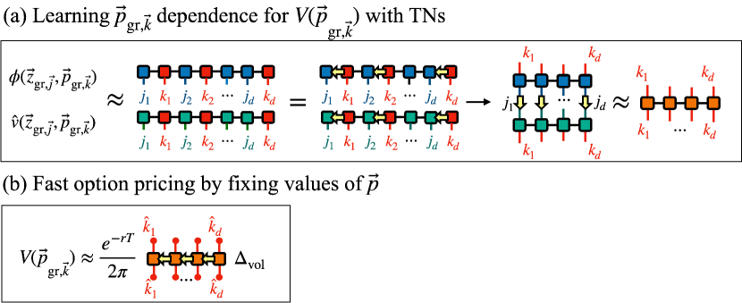
Figure 1: Fast option pricing based on TNs proposed in this study. In (a), we learn TTs with the parameter dependence of the functions using TCI and reduce the bond dimension of these TTs using SVD. We then contract the tensors associated with $p_{m}$ and $z_{m}$, resulting in two MPOs. We then take the contraction of these two MPOs with respect to the index vector $\vec{j}$ and compress the bond dimension of the resulting MPO using SVD. In (b), we use this MPO to perform fast option pricing for a specified parameter $\vec{p}$.

4.2 Computational complexity

The computational complexity of TT-based option pricing, involving computation for obtaining the specific tensor components $O^{\hat{k}_{1},\ldots,\hat{k}_{d}}_{\hat{k}_{1},\ldots,\hat{k}_{d}}$ for the fixed values of $\hat{k}_{1},\ldots,\hat{k}_{d}$ is $O(d\chi_{O}^{2})$ [26]. Here, we denote the maximum bond dimensions as $\chi_{K}$ In fact, the bond dimension depends on the bond index, and it is necessary to account for this for an accurate evaluation of the number of operations. Indeed, we consider this point in evaluating the computational complexity of TT-based option pricing demonstrated in Sec. V.

Here, we ignore the computational complexity of all the processes in FIG. 1 (a) and consider that in FIG. 1 (b) after we get the MPO only. This is reasonable if we can use plenty of time to perform these tasks before we need fast option pricing. As discussed in Sec. 6, we can reasonably find such a situation in practice.

5 Numerical demonstration

5.1 Details

Now, as a demonstration, we apply the proposed method to pricing a $d$-asset European min-call option in the BS model. In the following, we describe the parameter values used in this study, the software used, and how the errors were evaluated.

Ranges of ${\sigma_{m}}$ and ${S_{m,0}}$

With respect to $\vec{p}$, on which the TTs learn the dependence of the functions $\phi$ and $\hat{v}$, we take the two test cases: $\vec{p}$ is the volatilities $\vec{\sigma}$ or the present asset prices $\vec{S}_{0}$. In the proposed method, we need to set the range in the space of $\vec{p}$ and the grid points in it. For each volatility $\sigma_{m}$, we set the range to $\sigma_{m}\in[0.15,0.25]$, where the center $\sigma_{m}=0.2$ is a typical value of Nikkei Stock Average Volatility Index [29] and the range width $\pm 0.05$ covers the changes in this index on most days. For each $S_{m,0}$, we set the range to $S_{m,0}\in[90,120]$, which corresponds to the 20% variation of the asset price centered at 100. The lower bound is set to not 80 but 90 because the price of the option we take as an example is negligibly small for $S_{0}<90$. For both $\sigma_{m}$ and $S_{m,0}$, we set 100 equally spaced grid points in the range, and so the total number of the grid points in the space of $\vec{p}$ is $100^{d}$.

Other parameters

The other parameters for option pricing are fixed to the values summarized in the table below.

$T$	$r$	$K$	$S_{0}$	$\alpha$	$\rho_{mm}$	$\rho_{mn(m\neq n)}$	$N$
$1$	$0.01$	$100$	$100$	$5/d$	$1$	$1/3$	$50$

Table 1: The parameters except $\vec{\sigma}$ and $\vec{S}_{0}$.

Integral step size

The spread of the characteristic function changes depending on the values of the parameters $\vec{p}$ and the number of assets. Accordingly, it is necessary to adjust the grid interval $\eta_{m}$ for integration in the wavenumber space.

For example, consider the case where $\vec{p}=\vec{\sigma}$. From Eq. (10), we see that for the current parameter values in TABLE 1, $\phi$ takes non-negligible value only when $\sigma_{m}z_{m}\lesssim 1$ for each $m$. It is necessary to ensure that the grid points cover the whole of such a region with a sufficiently fine interval. Currently, as $z_{m}$ ranges from $-N\eta$ to $+N\eta$ with step size $\eta_{m}$, $\eta_{m}$ and $\sigma_{m}$ must satisfy $\sigma_{m}\eta_{m}\ll 1$ and $\sigma_{m}\times N\eta_{m}\gg 1$. Therefore, in general, we need the adjustment that $\eta_{m}$ increases when $\sigma$ decreases and vice versa. Nevertheless, in almost all the cases we tested, we observed that we get the accurate option price with $\eta_{m}$ set to some constant, and thus we did so. In the cases with $d=10,11$, $\eta_{m}$ is adjusted as

$$\eta_{m}=\frac{a}{\sigma_{m}}+b$$ (19)

To set the constants $a$ and $b$, we ran TT-based option pricing for several values of $\sigma_{m}$ adjusting $\eta_{m}$, found the pairs $(\sigma_{m},\eta_{m})$ that yields the accurate price, and adjust $a$ and $b$ so that Eq. (19) approximately reproduces such $\eta_{m}$ from $\sigma_{m}$.

Also when $\vec{p}=\vec{S}_{0}$, we set $\eta_{m}$ to some constant in almost all the test cases. Only for $d=11$, we try the adjustment that

$$\eta_{m}=\frac{\alpha}{S_{m,0}}+\beta$$ (20)

with $\alpha$ and $\beta$ chosen according to the option pricing result for several $\eta_{m}$ and $\sigma_{m}$. In general, larger $S_{m,0}$, which means larger $x_{m,0}$, makes $\phi$ as a function of $z_{m}$ oscillate more rapidly, and thus we need finer grid points to resolve such an oscillation.

Note that when $\eta_{m}$’s are set constant, the grid points do not depend on $\vec{p}$, and thus we can take the tensor $\hat{v}_{j_{1},\ldots,j_{d}}$ and its TT approximation $\tilde{v}_{j_{1},\ldots,j_{d}}$ having only the indexes $j_{1},\ldots,j_{d}$ associated with $z_{1},\ldots,z_{d}$.

Error evaluation

We do not have the exact price of the multivariate min-call option since there is no known analytic formula for it. Instead, we regard the option price computed by the MC-based method with very many paths, concretely $5\times 10^{7}$ paths, as the true value. The error of the option price computed by the proposed method is evaluated by its deviation from the true value. We take the MC-based method with $10^{5}$ paths, which is a typical number in option pricing in practical business, as the comparison target against our method. The average relative error and its standard deviation of the MC-based method with $10^{5}$ paths are calculated from its 20 runs. We assess the accuracy of our method by seeing if it falls within the statistical error range of the MC-based method.

An issue is that the number of possible combinations of the parameter $\vec{p}$ is $100^{d}$, and thus we cannot test all of them. Thus, we randomly select 100 combinations and perform option pricing for each of them. We compare the maximum among the relative errors of our method for the 100 parameter sets with the one obtained from the Monte Carlo simulations with the same parameter setting.

Software and hardware used in this study

TensorCrossInterpolation.jl for TCI [30] has not yet been made publicly available. Marc K. Ritter, Hiroshi Shinaoka, and Jan von Delft provided us with access to this. ITensors.jl [31] was utilized for computing the contraction and inner product of the tensor trains. The Monte Carlo simulations were carried out using tf-quant-finance [32]. Parallelization was not employed in either case. GPUs were not utilized in any of the calculations. The computations were performed on a 2019 MacBook Pro featuring a 2.3GHz 8-core Intel Core i9 processor and 16GB of 2667MHz DDR4 memory.

5.2 Results

We show the results for the computational complexity, time, and accuracy of TT-based and MC-based option pricing when two parameters $\vec{\sigma}$ and $\vec{S_{0}}$ are varied.

The results are summarized in TABLE 2. In particular, the computational complexity versus $d$ is plotted in FIG. 2. The maximum relative error of TT-based option pricing among runs for 100 random parameter sets is represented by $r_{\mathrm{TT}}$. The average relative error and standard deviation of the 20 runs of the MC-based method for the same parameter sets are denoted by $r_{\mathrm{MC}}$ and $\sigma_{\text{MC}}$, respectively. The computational complexities of TT-based and MC-based option pricing are represented by $c_{\mathrm{TT}}$ and $c_{\mathrm{MC}}$, respectively. Also, the computational time of TT-based and MC-based option pricing are denoted as $t_{\mathrm{TT}}$ and $t_{\mathrm{MC}}$, respectively. To maintain the desired accuracy of option pricing, we set the tolerance of TCI sufficiently low, concretely $\epsilon_{\mathrm{TCI}}=10^{-9}$ for $d\leq 10$, and $\epsilon_{\mathrm{TCI}}=10^{-10}$ for $d=11$. Subsequently, we reduce the bond dimension by SVD, with the tolerance of SVD set to $\epsilon_{\mathrm{SVD}}$ in TABLE 2 for $\phi$ and $\hat{v}$, respectively. The maximum bond dimensions of the MPOs for $\phi$ and $\hat{v}$ are denoted as $\chi_{\phi}$ and $\chi_{\hat{v}}$, respectively, in TABLE 2. We set the tolerance of SVD for obtaining $\chi_{K}$, maximum bond dimension of $O^{k_{1},\ldots,k_{d}}_{k_{1},\ldots,k_{d}}$, set to $\epsilon^{O}_{\mathrm{SVD}}=10^{-10}$ regardless of the number of assets to maintain the accuracy.

5.2.1 The case of varying $\vec{\sigma}$

TABLE 2 (a) shows the computational results of TT-based option pricing when we consider $\vec{\sigma}$ dependence. TT-based option pricing demonstrates advantages in terms of computational complexity and time over the MC-based method. The bond dimensions of the TT results for $d=5$ and $d=10$ are depicted in Fig. 3(a). By applying SVD to the TTs trained via TCI, the bond dimensions between tensors related to $p_{m}$ and $z_{m+1}$ could generally be maintained at less than 10. The details of this compression by SVD are described in Appendix A. The maximum bond dimension $\chi_{O}$ of $O^{k_{1},\ldots,k_{d}}_{k_{1},\ldots,k_{d}}$ is maintained at a small value of about 5, when $\eta$ is constant, but increases to about 20 when $\eta$ is automatically determined for each asset, which leads to increased computational complexity at around $d=10$. Still, the computational complexity is much lower than that of MC-based option pricing. The accuracy of the TT-based option pricing fell within the error range of the Monte Carlo method with $10^{5}$ paths.

It has been observed that accuracy tends to decrease as $d$ increases. Consequently, increasing $d$ further might result in decreased accuracy, making it difficult to maintain accuracy within the MC-based method.

Furthermore, reducing the number of subdivisions below 100 resulted in only minor changes in accuracy and computational complexity.

(a) $\vec{\sigma}$

$d$	$\eta$	$\epsilon_{\mathrm{SVD}}$	$r_{\mathrm{TT}}$	$r_{\mathrm{MC}}+\sigma_{\text{MC}}$	$c_{\mathrm{TT}}$	$c_{\mathrm{MC}}$	$t_{\mathrm{TT}}$[sec]	$t_{\mathrm{MC}}$[sec]	$\chi_{\phi}$	$\chi_{\hat{v}}$	$\chi_{O}$
$5$	0.9	$6.0\times 10^{-5}$	0.0162	0.0207	$43$	$5.0\times 10^{5}$	$3.12\times 10^{-5}$	$2.84\times 10^{-2}$	$4$	$7$	$4$
$6$	0.75	$5.0\times 10^{-5}$	0.0231	0.0254	$75$	$6.0\times 10^{5}$	$3.58\times 10^{-5}$	$3.38\times 10^{-2}$	$5$	$7$	$5$
$7$	0.69	$1.8\times 10^{-5}$	0.0203	0.0236	$70$	$7.0\times 10^{5}$	$4.13\times 10^{-5}$	$3.71\times 10^{-2}$	$6$	$7$	$4$
$8$	0.66	$2.0\times 10^{-5}$	0.0179	0.0253	$73$	$8.0\times 10^{5}$	$4.58\times 10^{-5}$	$4.09\times 10^{-2}$	$6$	$7$	$4$
$9$	0.61	$1.0\times 10^{-5}$	0.0240	0.0258	$89$	$9.0\times 10^{5}$	$5.15\times 10^{-5}$	$4.51\times 10^{-2}$	$7$	$7$	$4$
$10$	auto	$5.0\times 10^{-6}$	0.0309	0.0357	$2359$	$1.0\times 10^{6}$	$6.68\times 10^{-4}$	$5.11\times 10^{-2}$	$7$	$7$	$19$
$11$	auto	$3.5\times 10^{-6}$	0.0341	0.0347	$2797$	$1.1\times 10^{6}$	$7.91\times 10^{-4}$	$5.04\times 10^{-2}$	$8$	$7$	$20$

(b) $\vec{S}_{0}$

$d$	$\eta$	$\epsilon_{\mathrm{SVD}}$	$r_{\mathrm{TT}}$	$r_{\mathrm{MC}}+\sigma_{\text{MC}}$	$c_{\mathrm{TT}}$	$c_{\mathrm{MC}}$	$t_{\mathrm{TT}}$[sec]	$t_{\mathrm{MC}}$[sec]	$\chi_{\phi}$	$\chi_{\hat{v}}$	$\chi_{O}$
$5$	0.9	$2.0\times 10^{-4}$	0.0328	0.0374	$81$	$5.0\times 10^{5}$	$3.37\times 10^{-5}$	$2.90\times 10^{-2}$	$4$	$6$	$6$
$6$	0.75	$7.0\times 10^{-5}$	0.0265	0.0279	$114$	$6.0\times 10^{5}$	$4.26\times 10^{-5}$	$3.28\times 10^{-2}$	$5$	$6$	$6$
$7$	0.64	$3.0\times 10^{-5}$	0.0308	0.0355	$139$	$7.0\times 10^{5}$	$3.61\times 10^{-5}$	$3.66\times 10^{-2}$	$6$	$7$	$6$
$8$	0.57	$1.0\times 10^{-5}$	0.0259	0.0340	$120$	$8.0\times 10^{5}$	$5.25\times 10^{-5}$	$3.93\times 10^{-2}$	$7$	$7$	$5$
$9$	0.53	$1.0\times 10^{-5}$	0.0311	0.0345	$163$	$9.0\times 10^{5}$	$5.12\times 10^{-5}$	$4.54\times 10^{-2}$	$7$	$7$	$5$
$10$	0.5	$3.0\times 10^{-6}$	0.0315	0.0414	$171$	$1.0\times 10^{6}$	$6.02\times 10^{-5}$	$4.93\times 10^{-2}$	$7$	$8$	$5$
$11$	auto	$1.0\times 10^{-7}$	0.0379	0.0401	$853$	$1.1\times 10^{6}$	$3.43\times 10^{-4}$	$5.28\times 10^{-2}$	$9$	$14$	$11$

Table 2: The results of TT-based option pricing incorporating (a) $\vec{\sigma}$ and (b) $\vec{S}_{0}$ dependence. Here, we set the ranges $\sigma_{m}\in[0.15,0.25]$ and $S_{m,0}\in[90,120]$, and place 100 equally spaced grid points within these ranges. The $\epsilon_{\mathrm{SVD}}$ in the table refers to selected values that reduce $c_{\mathrm{TT}}$ keeping $r_{\mathrm{TT}}$ within the error range of MC-based option pricing $r_{\mathrm{MC}}+\sigma_{\text{MC}}$. The term auto in (a) and (b) indicate that $\eta_{m}$ was automatically determined for each asset based on Eqs. (19) and (20), respectively. The computational complexity and time increases when $\eta$ is set by Eq. (19) or (20). $t_{\mathrm{TT}}$ and $t_{\mathrm{MC}}$ represent the average computational time from 100 measurements, respectively.

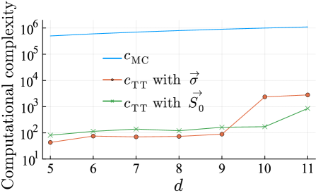
Figure 2: The computational complexity of TT-based and MC-based option pricing, denoted as $c_{\mathrm{TT}}$ and $c_{\mathrm{MC}}$, versus the number of assets $d$. We consider including parameter dependencies on $\vec{\sigma}$ and $\vec{S_{0}}$ in TTs. In TT-based option pricing with $\vec{\sigma}$ and $\vec{S_{0}}$, the sharp increase in computational complexity at $d=10$ and $d=11$ arises, respectively. This stems from the necessity to set $\eta$ by Eq. (19) or (20), which in turn makes the tensor $\hat{v}_{j_{1},k_{1},\ldots,j_{d},k_{d}}$ have indexes $k_{m}$ for $\vec{p}$.

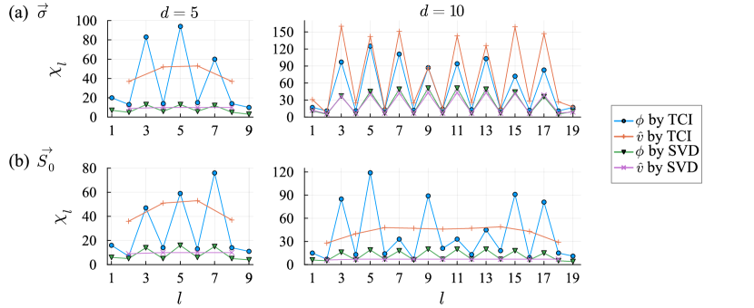
Figure 3: The bond dimensions $\chi_{l}$ of each bond $l$ for $\phi$ and $\hat{v}$, obtained through TCI and SVD, incorporating dependencies on (a) $\vec{\sigma}$ and (b) $\vec{S}_{0}$. The odd bond $l=2i-1$ connects the core tensors for $j_{m}$ and $k_{m}$, the indexes for $z_{m}$ and $p_{m}$, respectively, and the even bond $l=2i$ connects those for $k_{m}$ and $j_{m+1}$. In the cases corresponding to the left panels and the bottom right panel, $\hat{v}$ does not depend on parameters, and thus the bond $l$ takes only even values $2i$ (connecting the core tensors for $z_{m}$ and $z_{m+1}$). It is noteworthy that the graph of bond dimensions exhibits a characteristic jagged shape. The bond dimensions between sites for $j_{m}$ and $k_{m}$, which are related to the same asset, are large, and the ones between sites for $k_{m}$ and $j_{m+1}$, which are related to different assets, are small.

5.2.2 The case of varying $\vec{S_{0}}$

TABLE 2 (b) shows the results of TT-based option pricing when we consider $\vec{S_{0}}$ dependence. TT-based option pricing demonstrates superiority over the Monte Carlo method in terms of computational complexity and time. For $d$=5 and 10, after compression using SVD and contractions, the bond dimensions between tensors related to $p_{m}$ and $z_{m+1}$ were reduced to around 10 (refer to Fig. 3(b)). The maximum bond dimension, $\chi_{O}$, of $K^{k_{1},\ldots,k_{d}}_{k_{1},\ldots,k_{d}}$ is about 6 when $\eta$ is constant, while it increases to 11 when $\eta$ is adjusted per asset, leading to higher computational complexity at about $d=11$. Nonetheless, we saw superiority over the Monte Carlo method in terms of computation complexity and time.

Compared to varying $\sigma$, its accuracy is worse at $d=10$.

5.2.3 Randomness in learning the TTs

Here, we mention the randomness in learning the TTs and the error induced by it. Since TCI starts with the randomly selected grid points, the accuracy of the TT-based method depends on these initial points. To assess such a fluctuation of the accuracy, for $d=10$, we evaluated the mean and standard deviation of the relative accuracy of the TT-based method in 20 runs, with initial points randomly selected in each. As a result, the mean was 0.0324 and the standard deviation was 0.0039, which indicates that the accuracy fluctuation of TT-based option pricing is very small. We should note that TCI is a heuristic method, and depending on the choice of the initial points, the learning might not work well. That is, the error defined by Eq. (3) might not go below the threshold. Here, with the tolerance for TCI/SVD fixed, if the maximum relative error exceeds 4%, we redo TCI and SVD. The aforementioned mean and standard deviation are computed from successful cases.

5.2.4 Total computational time for obtaining the MPOs

Lastly, let us mention the total computational time for obtaining the MPOs for $\phi$ and $\hat{v}$ and $O^{k_{1},\ldots,k_{d}}_{k_{1},\ldots,k_{d}}$ through TCI and SVD. We focus on TCI because it dominates over SVD. It took about 3.4 hours for $d=11$ in the case that $\vec{\sigma}$ dependence is involved. This is sufficiently short for a practical use-case of the TT-based method mentioned exemplified in Sec. 6. We also note that, when we do not incorporate the parameter dependence into the tensor networks for $\phi$ and $\hat{v}$ as in [6], TCI takes a much longer time than the MC-based method, 7.3 seconds for $d=11$ in the case of $\vec{\sigma}$ dependence. In this setup, we set $\eta=0.48$, $\epsilon_{\mathrm{TCI}}=10^{-6}$ and all other parameters are the same as those in the default settings listed in Table 1. This means that running TCI every time the parameter varies does not lead to the time advantage of the TT-based method over the MC-based one.

6 Summary and discussion

We propose a method that employs a single TCI to learn TTs incorporating parameter dependence from functions of Eqs. (10) and (12), enabling fast option pricing in response to varying parameters. In this study, we considered scenarios with varying volatility and present stock prices as benchmarks for our proposed method. Up to $d=11$, we demonstrated superiority in both computational complexity and time. Here, we argue that, in principle, given at least comparable computational complexity, TT-based option pricing has an advantage in terms of computational time. This is because the TT-based method involves only multiplication and addition as unit operations, while the MC-based method requires more complex operations, such as random number generation and exponentiation, to be iterated $dN_{\rm path}$ times. However, in our demonstration, compared to the huge computational complexity advantage, the computational time advantage of TT-based option pricing is milder. This is because the TT-based method is bottlenecked by specifying the values of $\vec{p}$. Specifically, accessing the memory for the specific tensor components $O^{\hat{k}_{1},\ldots,\hat{k}_{d}}_{\hat{k}_{1},\ldots,\hat{k}_{d}}$ for the fixed values of $\hat{k}_{1},\ldots,\hat{k}_{d}$ dominates the computational time for additions and multiplications in tensor contraction. Therefore, in the TT-based method, and perhaps the MC-based method too, the implementation may have room for improvement to reduce computational time.

We also numerically verified that all TT-based results fell within the statistical error range of the Monte Carlo method with $10^{5}$ paths. However, it should be noted that increasing $d$ worsens accuracy, indicating a tendency for the accuracy to be worse than that of the MC-based method around $d\geq 12$.

Now, let us consider how the proposed method provides benefits in practical business in financial firms. An expected way to utilize this method is as follows. At night, when the financial market is closed, we learn the TTs and perform contractions, and then, during the day, when the market is open, we use the MPO to quickly price the option for the fluctuating parameters. If we pursue the computational speed in the daytime and allow the overnight precomputation to some extent, the above operation can be beneficial. In light of this, it is reasonable that we compare the computational complexity in the TT-based method after the TTs are obtained with that in the MC-based method, neglecting the learning process and contraction.

Finally, we discuss future research directions. If we could keep $\eta$ constant when $d$ is increased, we have the advantage of reducing the computational complexity involved in option pricing. It may be possible to keep $\eta$ constant by adjusting the value of parameter $N$, e.g. by increasing $N$ from the current value of 50 to, say, 100. It is a promising approach to directly learning the MPOs incorporating parameter dependence using TCI, potentially improving the accuracy of option pricing. At the same time, it is important to study methods to improve the numerical stability and accuracy of TCI itself. For our method to be more practical, compressing all the input parameters including both $\vec{\sigma}$ and $\vec{S}_{0}$ into a single TN format is desired, although this study tried to incorporate either of them as the first step. Expanding the methodology to other types of option calculations, particularly the application to American options, is also an important research direction.

Appendix A How to set the tolerance $\epsilon_{\mathrm{SVD}}$

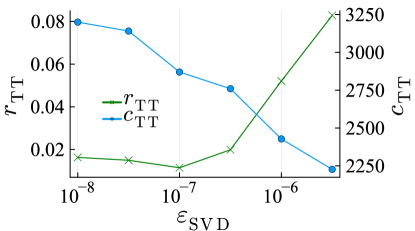
Figure 4: The maximum relative error $r_{\mathrm{TT}}$ and computational complexity $c_{\mathrm{TT}}$ when applying SVD with various $\epsilon_{\mathrm{SVD}}$ values to the TTs under the parameter settings of $d=10,\vec{\sigma},\eta=\text{auto}$. The left vertical axis represents $r_{\mathrm{TT}}$, while the right vertical axis shows $c_{\mathrm{TT}}$.

Figure 4 shows the maximum relative error $r_{\mathrm{TT}}$ and computational complexity $c_{\mathrm{TT}}$ when applying SVD with varying $\epsilon_{\mathrm{SVD}}$ to the TT with parameters for $d=10,~{}\vec{\sigma}$, obtained through TCI. Here, we fixed the tolerance of SVD $\epsilon^{O}_{\mathrm{SVD}}$ to $10^{-10}$. The tolerance $\epsilon_{\mathrm{SVD}}$ for SVD was chosen to maintain $r_{\mathrm{TT}}$ smaller than $r_{\mathrm{MC}}+\sigma_{\text{MC}}$, while minimizing the computational complexity $c_{\mathrm{TT}}$. From Fig. 4, it can be seen that $r_{\mathrm{TT}}$ increases sharply between $\epsilon_{\mathrm{SVD}}=10^{-6}$ and $10^{-5}$, suggesting that setting $\epsilon_{\text{SVD}}$ around $5.0\times 10^{-5}$ is appropriate for keeping $r_{\mathrm{TT}}$ smaller than $r_{\mathrm{MC}}+\sigma_{\text{MC}}$ while minimizing the computational complexity. By compressing the bond dimension with SVD, the computational time for the contraction of these optimized TTs also can be kept low.

From the fact that we can keep the maximum relative error $r_{\mathrm{TT}}$ small through SVD, it is suggested that the TTs obtained by TCI contain redundant information. By using SVD to get an optimal approximation in terms of the Frobenius norm, the reduced redundant information could be effectively removed. In addition, it is surprising that in the analysis with $\epsilon_{\text{SVD}}=10^{-6}$, the maximum relative error decreased compared to before compression by SVD. We consider that the error contained in TTs obtained by TCI is eliminated through SVD by chance. We expect that this phenomenon does not occur generally, and in fact, it did not occur for other asset numbers or parameters.

References

- [1] J. C. Hull, Options futures and other derivatives, Pearson (2003).
- [2] S. E. Shreve, Stochastic calculus for finance I & II, Springer (2004).
- [3] D. Herman, C. Googin, X. Liu, Y. Sun, A. Galda, I. Safro, M. Pistoia and Y. Alexeev, Quantum computing for finance, Nature Reviews Physics 5(8), 450 (2023), 10.1038/s42254-023-00603-1.
- [4] A. Montanaro, Quantum speedup of monte carlo methods, Proc. R. Soc. A 471(2181), 20150301 (2015), 10.1098/rspa.2015.0301.
- [5] K. Glau, D. Kressner and F. Statti, Low-rank tensor approximation for chebyshev interpolation in parametric option pricing, SIAM Journal on Financial Mathematics 11(3), 897 (2020), 10.1137/19M1244172, https://doi.org/10.1137/19M1244172.
- [6] M. Kastoryano and N. Pancotti, A highly efficient tensor network algorithm for multi-asset fourier options pricing (2022), 2203.02804.
- [7] R. Patel, C.-W. Hsing, S. Sahin, S. S. Jahromi, S. Palmer, S. Sharma, C. Michel, V. Porte, M. Abid, S. Aubert, P. Castellani, C.-G. Lee et al., Quantum-inspired tensor neural networks for partial differential equations (2022), 2208.02235.
- [8] C. Bayer, M. Eigel, L. Sallandt and P. Trunschke, Pricing high-dimensional bermudan options with hierarchical tensor formats, SIAM Journal on Financial Mathematics 14(2), 383 (2023), 10.1137/21M1402170, https://doi.org/10.1137/21M1402170.
- [9] I. V. Oseledets, Tensor-train decomposition, SIAM Journal on Scientific Computing 33(5), 2295 (2011), 10.1137/090752286.
- [10] P. Carr and D. Madan, Option valuation using the fast fourier transform, Journal of computational finance 2(4), 61 (1999).
- [11] A. L. Lewis, A simple option formula for general jump-diffusion and other exponential lévy processes, Available at SSRN 282110 (2001).
- [12] R. Orús, A practical introduction to tensor networks: Matrix product states and projected entangled pair states, Annals of Physics 349, 117 (2014), https://doi.org/10.1016/j.aop.2014.06.013.
- [13] K. Okunishi, T. Nishino and H. Ueda, Developments in the tensor network — from statistical mechanics to quantum entanglement, Journal of the Physical Society of Japan 91(6), 062001 (2022), 10.7566/JPSJ.91.062001.
- [14] E. Stoudenmire and D. J. Schwab, Supervised learning with tensor networks, In D. Lee, M. Sugiyama, U. Luxburg, I. Guyon and R. Garnett, eds., Advances in Neural Information Processing Systems, vol. 29. Curran Associates, Inc. (2016).
- [15] A. Novikov, M. Trofimov and I. Oseledets, Exponential machines, arXiv preprint arXiv:1605.03795 (2016).
- [16] H. Shinaoka, M. Wallerberger, Y. Murakami, K. Nogaki, R. Sakurai, P. Werner and A. Kauch, Multiscale Space-Time ansatz for correlation functions of quantum systems based on quantics tensor trains, Phys. Rev. X 13(2), 021015 (2023), 10.1103/PhysRevX.13.021015.
- [17] Y. Núñez Fernández, M. Jeannin, P. T. Dumitrescu, T. Kloss, J. Kaye, O. Parcollet and X. Waintal, Learning feynman diagrams with tensor trains, Phys. Rev. X 12(4), 041018 (2022), 10.1103/PhysRevX.12.041018.
- [18] H. Takahashi, R. Sakurai and H. Shinaoka, Compactness of quantics tensor train representations of local imaginary-time propagators (2024), 2403.09161.
- [19] E. Ye and N. F. G. Loureiro, Quantum-inspired method for solving the vlasov-poisson equations, Phys. Rev. E 106, 035208 (2022), 10.1103/PhysRevE.106.035208.
- [20] I. Oseledets and E. Tyrtyshnikov, TT-cross approximation for multidimensional arrays, Linear Algebra Appl. 432(1), 70 (2010), 10.1016/j.laa.2009.07.024.
- [21] S. Dolgov and D. Savostyanov, Parallel cross interpolation for high-precision calculation of high-dimensional integrals, Comput. Phys. Commun. 246, 106869 (2020), 10.1016/j.cpc.2019.106869.
- [22] M. K. Ritter, Y. Núñez Fernández, M. Wallerberger, J. von Delft, H. Shinaoka and X. Waintal, Quantics tensor cross interpolation for High-Resolution parsimonious representations of multivariate functions, Phys. Rev. Lett. 132(5), 056501 (2024), 10.1103/PhysRevLett.132.056501.
- [23] A. Shashua and A. Levin, Linear image coding for regression and classification using the tensor-rank principle, In Proceedings of the 2001 IEEE Computer Society Conference on Computer Vision and Pattern Recognition. CVPR 2001, vol. 1, pp. I–I, 10.1109/CVPR.2001.990454 (2001).
- [24] M. A. O. Vasilescu and D. Terzopoulos, Multilinear analysis of image ensembles: Tensorfaces, In A. Heyden, G. Sparr, M. Nielsen and P. Johansen, eds., Computer Vision — ECCV 2002, pp. 447–460. Springer Berlin Heidelberg, Berlin, Heidelberg, ISBN 978-3-540-47969-7 (2002).
- [25] I. G. Ion, C. Wildner, D. Loukrezis, H. Koeppl and H. De Gersem, Tensor-train approximation of the chemical master equation and its application for parameter inference, The Journal of Chemical Physics 155(3), 034102 (2021), 10.1063/5.0045521, https://pubs.aip.org/aip/jcp/article-pdf/doi/10.1063/5.0045521/13511567/034102_1_online.pdf.
- [26] U. Schollwock, The density-matrix renormalization group in the age of matrix product states, Ann. Phys. 326(1), 96 (2011), 10.1016/j.aop.2010.09.012.
- [27] K. G. Ernst Eberlein and A. Papapantoleon, Analysis of fourier transform valuation formulas and applications, Applied Mathematical Finance 17(3), 211 (2010), 10.1080/13504860903326669.
- [28] P. Glasserman, Monte Carlo methods in financial engineering, vol. 53, Springer (2004).
- [29] https://indexes.nikkei.co.jp/en/nkave/index/profile?idx=nk225vi.
- [30] Y. Núñez Fernández, M. K. Ritter, M. Jeannin, J.-W. Li, T. Kloss, O. Parcollet, J. von Delft, H. Shinaoka and X. Waintal, In preparation (2024).
- [31] M. Fishman, S. R. White and E. M. Stoudenmire, The ITensor Software Library for Tensor Network Calculations, SciPost Phys. Codebases p. 4 (2022), 10.21468/SciPostPhysCodeb.4.
- [32] Google, tf-quant-finance, https://github.com/google/tf-quant-finance (2023).