A highly efficient tensor network algorithm for multi-asset Fourier options pricing

Abstract

Risk assessment and in particular derivatives pricing is one of the core areas in computational finance and accounts for a sizeable fraction of the global computing resources of the financial industry. We outline a quantum-inspired algorithm for multi-asset options pricing. The algorithm is based on tensor networks, which have allowed for major conceptual and numerical breakthroughs in quantum many body physics and quantum computation. In the proof-of-concept example explored, the tensor network approach yields several orders of magnitude speedup over vanilla Monte Carlo simulations. We take this as good evidence that the use of tensor network methods holds great promise for alleviating the computation burden of risk evaluation in the financial and other industries, thus potentially lowering the carbon footprint these simulations incur today.

I Introduction

Options pricing remains an active field of research and development in financial engineering. In its simplest form, an option is a contract which allows the buyer to purchase some specified underlying financial asset, such as stock, bonds, etc. at a given strike price at a specified expiration date. The central task of options pricing is to evaluate what the fair price is for such a contract, such that arbitrage—the possibility to make a profit at no risk—is impossible. A great number of variants to this simple setting exist, including functions of several assets, multiple expiration dates, and time dependent returns [1]. Derivative products are essential for investors seeking to expand their investment and hedging strategies, and have constituted an especially fluid market for decades. Given the large volume and diversity of derivatives products being traded on the financial markets, understanding their properties is an essential objective of financial engineering.

Only the very simplest options pricing scenarios can be evaluated analytically. Therefore, in general, one has to resort to numerical simulations. These typically break up into two general approaches: Either approximate the solution via Monte Carlo or Fourier methods, building upon the general Feynman-Kac formulation of the solution, or map the stochastic differential equation (SDE) describing the dynamics to a partial differential equation (PDE), and subsequently solve the continuous PDE with appropriate boundary conditions and a discretization scheme. In this work we do not consider the PDE-based approach.

Monte Carlo methods are generally simple to implement and are very versatile, but have a rather slow sample convergence rate that is proportional to the inverse square root of measurements $n$, i.e. of ${\mathcal{O}}(1/\sqrt{n})$. Quasi-Monte Carlo methods can in certain cases improve the scaling to close to ${\mathcal{O}}(1/n)$ [2, 3], but their accuracy and reliability is on a case by case basis. Monte Carlo methods also have the significant advantage that they typically do not suffer from the curse of dimensionality—that is, the effort scales exponentially in the space dimension—and are thus the only numerical method available for multi-asset pricing scenarios. Furthermore, Monte Carlo methods also struggle with complex path-dependent options where the computations can no longer be parallelized easily.

The main focus in this article is on the Fourier method of options pricing. This numerical approach is typically many orders of magnitude faster than any other on single assets, when applicable. For this reason, it is sometimes referred to as an exact method. However, it suffers severely from the curse of dimensionality. See Ref. [4] for standard comparisons of the different numerical approaches to simple options of a single asset.

A number of proposals have recently appeared [5, 6, 7, 8, 9] suggesting a quantum advantage for the options pricing problem. Most of them are based on the work by Montanaro [10] showing that Monte Carlo sampling can be performed on a quantum computer with an ${\mathcal{O}}(1/n)$ convergence rate. However, the algorithm requires a fault-tolerant quantum computer because it is based on quantum phase estimation (QPE), which requires a circuit depth that is well beyond the reach of currently-available noisy intermediate-scale quantum (NISQ) devices. Furthermore, it is unclear whether the QPE approach will ever be competitive given the modest polynomial scaling advantage, the large overhead of fault-tolerant quantum computing and the competing classical quasi-Monte Carlo methods. Chakrabarti et. al [7] argue that for exotic options there will be a threshold where QPE provides an advantage which is of the same order of magnitude as that argued for in quantum chemistry. A different approach proposes to solve the PDE associated with an option [8], yet, in view of a careful analysis of quantum algorithms for differential equations [11, 12], falsely claim an exponential speedup.

In this paper we consider an approach to the multi-asset options pricing problem that is loosely inspired by quantum computing. We start from the Fourier formulation of the multi-asset problem and formulate it as the inner product of two complex vectors: one representing the characteristic function of the stochastic dynamics and one representing the Fourier transform of the payoff. The two vectors are approximately built as nonnormalized matrix product states (MPS) via the TT-cross [13] algorithm. The inner product can then be evaluated efficiently and thus multi-asset options pricing accelerated accordingly.

On a correlated multi-asset example, we find that our algorithm accurately matches the exact results up to $4$ assets with dramatically reduced computational time. Beyond that it matches Monte Carlo-based results and provides a significant speedup for up to $15$ assets. Our approach can be applied to many practical options pricing scenarios, and therefore holds great promise for practical computational speedup.

The paper is structured as follows. Section II introduces the European call option, followed by an outline of Monte Carlo and Fourier-based options pricing in Sec. III. Section IV then presents the quantum formulation of the problem, as well as a solution using tensor networks. Numerical experiments are shown in Sec. V, followed by concluding remarks.

II The European call option

The European call option is a contract established between a buyer and a seller relating to an underlying asset (bond, stock, interest rate, currency, etc.). The contract allows the buyer to purchase the underlying asset at a specific strike price $K$ at the termination date $T$. The buyer has no obligation to purchase the underlying asset. Therefore, given an asset price $S_{0}$ at time $t=0$, a strike price $K$ and a termination date $T$, the value of the option at time $T$ is

$$v(S_{T},K)=\max\{S_{T}-K,0\},$$ (1)

for the specific (random) trajectory of the asset starting at price $S_{0}$ and ending at price $S_{T}$. The main challenge in options pricing is to determine the value of the option at time $t\leq T$. The Feynman-Kac formula provides a mathematically precise answer to this problem, namely

$$V(t,K|S_{0})=e^{-r(T-t)}\mathbb{E}[v(S_{T},K)|S_{0}],$$ (2)

where $e^{-r(T-t)}$ accounts for a constant discount $r$ with a risk-free investment such as a bond. The expectation is over all stochastic trajectories of the underlying asset starting at $S_{0}$. The discounted price, Eq. (2) is a Martingale measure under the no-arbitrage assumption [1].

We start with the simplest model, namely the Black-Scholes model with one underlying asset. The model is defined either in SDE or PDE setting. Let $S_{t}$ be the value of an underlying asset at time $t\geq 0$. Under geometric Brownian motion, the time evolution is described by the SDE

$$dS_{t}=rS_{t}dt+\sigma S_{t}dW_{t},$$ (3)

where $r$ is a constant rate of return, and $\sigma$ a variance called the volatility. Black and Scholes showed [14] that the dynamics of the European put option under geometric Brownian motions can be cast as the PDE of the form

$$\frac{\partial V(t,S)}{\partial t}+\frac{1}{2}\sigma^{2}S^{2}\frac{\partial^{2}V(t,S)}{\partial S^{2}}+rS\frac{\partial V(t,S)}{\partial S}=0,$$ (4)

where $V(t,S)$ describes the price of the asset at time $t>0$, subject to the termination condition

$$V(T,S_{T})=\max\{S_{T}-K,0\}.$$ (5)

In the PDE setting one wants to solve the inverse time problem, i.e., given a boundary condition at time $t=T$, find the solution at time $t=0$. In this very special case, there exists an exact solution (known as the the Black Scholes solution) given by

$$V(t,S_{0})=S_{0}\Phi(d_{1})-Ke^{-r(T-t)}\Phi(d_{2}),$$ (6)

where

$$\Phi(x)=\frac{1}{\sqrt{2\pi}}\int_{-\infty}^{x}e^{-s^{2}/2}ds$$ (7)

and

$$d_{1/2}=\frac{\ln(S_{0}/K)+(r\pm\sigma^{2}/2)(T-t)}{\sigma\sqrt{T-t}}.$$ (8)

In the early days of electronic options trading, most options were priced using this formula because it was accurate and simple to compute. However, following the stock market crash of 1989, practitioners realised that the Black-Scholes model did not account for the “volatility smile,” rather assuming that the volatility is constant and independent of the strike price. More sophisticated models are used today that better account for the heavy tailed distribution of financial assets, such as, for example, the SABR model [15]. However, the Black-Scholes model remains the conceptual building block behind much of options pricing. Unfortunately, the more sophisticated models and payoff functions do not allow for analytic solutions and one must resort to numerical estimations.

II.1 Multi-asset extension

We consider a multi-asset extension of the European put option under geometric Brownian motion. Let $\vec{S_{t}}=\{S_{t}^{1},...,S_{t}^{d}\}$ denote the prices of $d$ underlying assets. The geometric Brownian motion can similarly be extended to the multi-asset scenario via

$$dS^{j}_{t}=rS^{j}_{t}dt+\sigma_{j}S^{j}_{t}dW^{j}_{t},$$ (9)

where the stochastic terms $\{dW_{t}^{j}\}$ have Gaussian correlations described by the correlation matrix

$$\mathbb{E}[dW^{j}_{t}dW^{j}_{t}]=\Sigma_{ij}dt.$$ (10)

We assume that the correlation matrix is positive definite throughout.

We consider a commonly-used multi-asset option, the min option, which returns the minimum of the underlying assets for a fixed strike price $K$:

$$v_{\min}(S_{T},K)=\max\{\min\{S_{T}^{1},...,S_{T}^{d}\}-K,0\}.$$ (11)

There are many other possible extensions to multiple assets. However, this is the simplest one that captures correlations both in the stochastic dynamics, as well as in the multi-asset option. In the correlated multi-asset case there no longer exists an analytic solution, so numerical simulations are needed. In practice, Monte Carlo methods are often used, because they do not suffer from the curse of dimensionality.

III Monte Carlo and Fourier simulations

III.1 Monte Carlo options pricing

In this section we succinctly describe the Monte Carlo and Fourier approaches to numerical options pricing. We start with the Feynman-Kac formula, and express the expectation as an integral over the conditional probability $p(S_{T}|S_{0})$ that the value of the asset at time $T$ is $S_{T}$ given that its value at time $t=0$ is $S_{0}$:

$$V(t,K|S_{0}) = e^{-r(T-t)}\int_{0}^{\infty}v(S_{T},K)p(S_{T}|S_{0})dS_{T}$$ (12)

$$= e^{-r(T-t)}\int_{-\infty}^{\infty}v(e^{x},K)p(x|x_{0})dx,$$ (13)

where in the second line we changed variables to $x=\ln(S_{T})$ and $x_{0}=\ln(S_{0})$. The change of variables reduces geometric Brownian motion to regular Brownian motion, where $p(x|x_{0})$ is the normal distribution with mean at $\mu=s_{0}/T+r-\sigma^{2}/2$ and standard deviation $\sigma$. The Monte Carlo approach to evaluate the integral in Eq. (13) is by sampling geometric Brownian motion trajectories according to Eq. (3), and averaging over the functional outcomes $v(e^{x},K)$:

• Simulate a trajectory ${\bf S}=\{S_{0},S_{\delta t},\cdots,S_{T}\}$, where $M=T\delta t$ is the number time points, by the discretization of the SDE in Eq. (3).

• Generate $n$ trajectories (samples) $\{{\bf S}^{(j)}\}_{j=1}^{N}$, and evaluate the function $v(S_{T},K)$ for each trajectory.

• Approximate

  $$\int_{-\infty}^{\infty}v(e^{x},K)p(x|x_{0})dx\approx\frac{1}{N}\sum_{j=1}^{N}v(S^{(j)}_{T},K)$$ (14)

While extremely natural and general for path independent options, the Monte Carlo approach converges rather slowly proportional to $O(1/\sqrt{n})$, where $n$ is the number of samples, making it computationally costly to obtain high-precision answers, especially when multiple strike prices are desired. Monte Carlo methods also struggle with time dependent options, where independent trajectories can no longer be used throughout the lifetime of the option [16].

III.2 Fourier options pricing

In Fourier options pricing, the probability density $p(x|x_{0})$ is constructed explicitly from the characteristic function $\varphi_{T}$ of the dynamics, via the relation

$$\varphi_{T}(u)=\mathbb{E}[e^{iuX_{T}}|X_{0}]=\int_{\mathbb{R}}e^{iux}p(x|x_{0})dx,$$ (15)

where $X_{t}$ is the random variable at time $t$ of the stochastic process described by Eq. (3).

The reason for working with the characteristic function is twofold. First, the conditional probability $p(x|x_{0})$ is only known analytically in very few special cases, while analytic expressions for the characteristic function are more widely known (e.g., Black-Scholes-Merton [17], Heston [18]) or can be approximated (e.g., SABR [15, 19]). Second, the function is more stable in the Fourier domain for small time steps due to the uncertainty principle.

We can substitute the inverse of Eq. (15) in Eq. (13) to obtain:

$$V(t,K|S_{0})=e^{-r(T-t)}\int_{\mathbb{R}^{2}}e^{-iux}v(e^{x},K)\varphi_{T}(u)dxdu.$$ (16)

This expression can be approximated numerically, but it suffers a rather large discretization error because $v(e^{x},K)$ is not square integrable in $\mathbb{R}$. To remedy this, Carr and Madan [20] have proposed a method of stabilising the nonintegrability by shifting the Fourier integration into the complex plane. We outline a slightly different approach due to Lewis [17], which generalizes more easily to the types of multi-dimensional payoffs that we consider.

The Lewis approach is based on taking the Fourier transform of the payoff function. Consider the case of the European call option $v_{\rm call}(z)$. Its Fourier transform is given by

$$\hat{v}_{\rm call}(z) = \int_{-\infty}^{\infty}e^{izx}\min\{e^{x}-K,0\}dx$$ (17)

$$= \left.\left(\frac{e^{(iz+1)x}}{iz+1}-K\frac{e^{izx}}{iz}\right)\right|_{\ln(K)}^{\infty}=\frac{-K^{iz+1}}{z(z-i)},$$ (18)

where $z$ is complex, and the last equation only holds in the strip ${\rm Im}[z]>1$, because the Fourier transform of the payoff function has a branch cut in the complex plane. The inverse transform can then be expressed as

$$v_{\rm call}(x)=\frac{1}{2\pi}\int_{-\infty+\alpha}^{\infty+i\alpha}e^{-izx}\hat{v}_{\rm call}(z)dz,$$ (19)

where $\alpha>1$ guarantees that the Fourier transform of the payoff is well defined. Clearly, different payoffs will have different domains of integrability. For a comprehensive analysis, see Refs. [21, 22]. We can then express the options price as:

$$V(t,K|S_{0}) = e^{-r(T-t)}\mathbb{E}[v_{\rm call}(X_{T})|X_{0}]$$ (20)

$$= \frac{e^{-r(T-t)}}{2\pi}\mathbb{E}[\int_{i\alpha-\infty}^{i\alpha+\infty}e^{-izX_{T}}\hat{v}_{\rm call}(z)dz|X_{0}]$$

$$= \frac{e^{-r(T-t)}}{2\pi}\int_{i\alpha-\infty}^{i\alpha+\infty}\mathbb{E}[e^{-izX_{T}}|X_{0}]\hat{v}_{\rm call}(z)dz$$

$$= \frac{e^{-r(T-t)}}{2\pi}\int_{i\alpha-\infty}^{i\alpha+\infty}\varphi_{T}(-z)\hat{v}_{\rm call}(z)dz$$

III.3 The multi-asset case

The Fourier method can easily be extended to the multi asset case provided the multi-asset characteristic function is known and the Fourier transform of the payoff can be evaluated explicitly. The characteristic function of multi-asset geometric Brownian motion is given by:

$$\varphi_{T}(\vec{z})=\exp\left[i\sum_{j}^{d}z_{j}\mu_{j}-\frac{1}{2}\sum_{j}^{d}\sum_{k}^{d}\sigma_{j}\sigma_{k}z_{j}z_{k}\Sigma_{jk})\right],$$ (21)

where

$$\mu_{j}=x^{j}_{0}+r_{j}T-\frac{1}{2}\sigma_{j}^{2}\Sigma_{jj}T,$$ (22)

with $j=1,...,d$. The Fourier transform of the min option is [22]:

$$\hat{v}_{\rm min}(\vec{z})=\frac{K^{1+i\sum_{j=1}^{d}z_{j}}}{(-1)^{d}(1+i\sum_{j=1}^{d}z_{j})\prod_{j=1}^{d}z_{j}},$$ (23)

and is subject to the conditions: ${\rm Im}[z_{j}]>0$ and $\sum_{j=1}^{d}{\rm Im}[z_{j}]>1$. Note that, $\hat{v}_{\min}$ reduces to the single asset formula when $d=1$. We can express the price of the multi-asset min option as

$$V(t,K|S_{0})=\frac{e^{-r(T-t)}}{2\pi}\int_{\mathbb{R}^{d}+i\vec{\alpha}}\varphi_{T}(-\vec{z})\hat{v}_{\rm min}(\vec{z})d\vec{z}.$$ (24)

III.4 Discretization

We now discuss the numerical evaluation of the single asset formula in Eq. (20). The multi-asset extension is straightforward. We first need to truncate the integral at a finite value. The probability distribution $p(x|x_{0})$ is Gaussian, so it can be well approximated on a finite square of size $[-a\sigma,a\sigma]$ around the mean, where the approximation improves exponentially in $a$. Typically $a=5$ yields good numerical precision. The discretization in real and Fourier space should satisfy the uncertainty relation: $dx\cdot dk=2\pi/N$. Given that $dx\propto 1/N$, we expect the Fourier increment to be constant. $dk$ is left as a free variable in our numerical experiments, and is typically taken to be of order $1$. Its value can heavily affect the accuracy of the result. The expression to evaluate is then

$$V(t,K|S_{0})\!=\!\frac{e^{-r(T-t)}}{2\pi}\!\!\!\!\!\!\sum_{j=-N/2}^{N/2}\!\!\!\varphi_{T}(-\eta j-i\alpha)\hat{v}_{\rm min}(\eta j+i\alpha)\eta,$$ (25)

where $\eta$ is identified with $dk$. We pause here to make an observation about the shift to the imaginary plane. One might naively expect that Eq. (25) is equivalent to the discretization of Eq. (13). Indeed, one could perform the shift to the complex plane as well as the discrete Fourier transform. However, the catch is that the discrete analogue of the delta function $(1/2\pi)\sum_{j}\exp[ij\eta(x-y)]$ is non-zero away from $x=y$, and gives rise to an error. In this way there is a very subtle numerical error that creeps up in the original expression Eq. (13), that has its roots in complex analysis.

Equation (25) yields exquisite precision already for small values of $N$ (see Sec. V). For that reason, it is often referred to as a quasi-exact method in the options pricing literature. Numerically simulating the multi-asset extension of Fourier pricing is straightforward by replacing the single sum by a nested sum. However, the evaluation of the nested sum becomes computationally prohibitive beyond a few assets. Indeed, building the vectors $\vec{\varphi}_{T}$ and $\hat{\vec{v}}_{\rm min}$ also becomes prohibitive beyond a few assets, scaling exponentially in the number of assets.

IV Quantum formulation and tensor network solution

We propose a quantum-inspired solution based on tensor networks which reduces the computational cost of multi-asset Fourier options pricing from ${\mathcal{O}}(N^{d})$ to ${\mathcal{O}}(dN)$. As shown in Sec.V, our method typically has the same asymptotic scaling as Monte Carlo, but with a prefactor several orders of magnitude smaller. The main idea is to express Eq. (24) or Eq. (13) as the inner product of two (nonnormalized) quantum states in matrix product form. In the case of Eq. (24) we obtain:

$$V(t,K|S_{0})=\frac{e^{-r(T-t)}}{2\pi}\langle\hat{v}_{\rm min}|\varphi_{T}\rangle,$$ (26)

where

$$|\varphi_{T}\rangle=\sum_{j_{1},...,j_{d}=-N/2}^{N/2}\varphi_{T}(-\eta\vec{j}-i\alpha)|\vec{j}\rangle,$$ (27)

and

$$|\hat{v}_{\rm min}\rangle=\sum_{j_{1},...,j_{d}=-N/2}^{N/2}\hat{v}_{\rm min}(-\eta\vec{j}-i\alpha)|\vec{j}\rangle.$$ (28)

For a single asset, working in Fourier space and shifting the integral sufficiently far off the real axis yields tremendous improvements in numerical accuracy[17]. We next show how to extend the speed and precision of the Fourier approach into the multi-asset regime. In order to make use of the quantum-inspired approach, we need an efficient representation of the vectors $|\varphi_{T}\rangle$ and $|\hat{v}_{\rm min}\rangle$ and an efficient way to perform the inner product in Eq. (26), as well as a way to efficiently prepare the vectors. If the vectors can be accurately represented as nonnormalized matrix product states (also known as tensor trains [23]), then the former will be satisfied. However, the latter is more challenging. Here, we adopt the black-box TT-cross algorithm [13, 24, 25] for efficiently preparing the states. Another candidate black-box solution to the problem is “tensor completion” [26]. For specific models, there are more reliable and faster solutions, for instance by solving the Fokker Planck equation using density matrix renormalization group (DMRG) methods, which we plan to explore in more detail elsewhere.

IV.1 Matrix Product States

A matrix product state (MPS) is a parametrized class of states (vectors normalized in $\ell_{2}$ norm) on an $N^{d}$ dimensional Hilbert space. These states are completely described by a set of $D\times D$ matrices $\{A^{j_{\alpha}}\}$, with $j=1,...,N$ and $\alpha=1,...,d$ as:

$$|\Psi\rangle=\sum_{j_{1},...,j_{d}}A^{j_{1}}\cdots A^{j_{d}}|j_{1},\cdots,j_{d}\rangle.$$ (29)

The MPS vector is therefore described completely by $2NdD^{2}$ real numbers, instead of $2N^{d}$ for the dense vector. Furthermore, the inner product between two MPS with identical bond dimension can be evaluated in ${\mathcal{O}}(2NdD^{2})$ operations. In our case, each site represents an asset, so $j_{\alpha}=-N/2,\cdots,N/2$. The matrices $\{A^{j_{\alpha}}\}$ carry the correlation between the assets for $|\varphi_{T}\rangle$. In numerical simulations, the stronger the correlations, the larger the bond dimension $D$ must be. In principle, in order to describe a random quantum state in a $d$-dimensional Hilbert space exactly, a bond dimension of $D=N^{d/2}$ is required, which is no simplification on the dense encoding. However, in most practical settings, including the one at hand, a small (constant) bond dimension suffices. In our numerical experiments in Sec. V.3, we have observed that a bond dimension of approximately $D=10$ — $15$ is often sufficient to capture the correlations of an arbitrary Gaussian state.

Finally, note that MPSs form the basis of the highly-effective DMRG algorithm in quantum many body physics [27] and in quantum chemistry [28]. They have also been applied to various problems in numerical and data analysis under the name of tensor trains [23].

IV.2 The TT-cross algorithm

The TT-cross algorithm [13] constructs an MPS representation of a multi-variate function with relatively few calls to the function. For example, a function $f:\mathbb{R}^{d}\rightarrow\mathbb{R}$ of $d$ variables can be discretized as a tensor with $d$ indices. If each variable is discretized on $N$ grid points, the tensor takes $N^{d}$ real values. Clearly, without strong promises on sparsity or rank, even for moderately large $N$ and $d$, the tensor cannot be written to memory or manipulated efficiently. If it can be accurately approximated by an MPS with small bond dimension, then the tensor becomes manageable. In general, it is not obvious how to build MPS representations just from oracular access to the function $f$. One strategy is to build the MPS by successive singular value decompositions and low-rank approximations of the full tensor [13]. The TT-cross algorithm solves this problem in a different way. The algorithm allows to approximate a nonnormalized MPS of specified bond dimension $D$ by accessing the function ${\mathcal{O}}(dND^{2})$ times [24], which can provide tremendous time savings, when $d$ and $N$ are large. The main benefit of the TT-cross algorithm over other black box constructions is that it builds the tensor out of actual entries of the original function, making it very well suited when oracular access to the function is computationally cheap. When, instead of arbitrary oracular access we are only given (unstructured) samples of the function, then tensor completion [26] is a better method of reconstructing the MPS from the data.

The main idea is to perform an iterated matrix cross optimization. The matrix cross identity states that a rank-$r$ $n\times m$ matrix $M$ can be decomposed as

$$M=M(:,J)M(I,J)^{-1}M(I,:),$$ (30)

where $J$, $I$ are sets of $r$ columns and rows, $M(:,J)$ is the matrix of $r$ columns indexed by $J$, and $M(I,J)$ is the sub-matrix of $M$ indexed by columns $J$ and rows $I$. When $r\ll m,n$, the representation is more economical. The expression is exact for a rank $r$ matrix and holds true for any choice of rows and columns. It is natural to ask what the best rank $r$ cross approximation is, when the matrix has rank larger than $r$. The answer is known to be the submatrix with the largest sub-volume $|\det(M(I,J))|$. Unfortunately, finding the largest submatrix is an NP-hard problem, so we need to resort to approximations.

A good heuristic approach to finding the largest volume is to start with a set of random columns $J$ , and obtain the $r$ rows leading to the largest volume submatrix of $M(:,J)$. This can be done efficiently using the maxvol algorithm [29]. Then starting from the rows found in the previous step, find the new columns that optimize $M(I,:)$. Performing this step iteratively quickly converges to a solution which is often close to the optimum.

The extension to rank-$D$ tensors is straightforward. Consider an MPS with $d$ sites, physical dimension $N$ and bond dimension $D$. Choose a set of rows $\{I_{1},...,I_{d}\}$ and columns $\{J_{1},...,J_{d}\}$, where each set $I_{\alpha},J_{\alpha}$ has $D$ elements chosen from $N$. Then, sweeping back and forth we can solve each matrix cross problem individually using the above heuristic method by keeping all other links in the tensor network fixed. In numerical experiments, it has been observed that the process converges after a small number of sweeps. Convergence is measured by generating $50000$ random sample points of the function and of the MPS approximation to the function, and evaluate the one-norm difference between the two. For a more comprehensive explanation of the TT-cross algorithm with pseudo-code, see Refs. [24] and [25].

V Numerical experiments

We now show that the tensor network approach to multi-asset Fourier options pricing faithfully extends the great precision of Fourier options pricing into the multi-asset regime. In all of our experiments, we set the parameters of the model to $r=0.3$, $\sigma=0.5$, and $T=1$. The strike price and starting asset price are set to $S_{0}=K=100$ homogeneously across all assets. These are fairly standard settings and serve to illustrate the general behaviour of the tensor network solver. The conclusions do not change qualitatively with different choices of parameters. Simulations are performed in python on a standard laptop without GPU acceleration. The TT-cross components used the package tntorch [30].

V.1 The single asset case

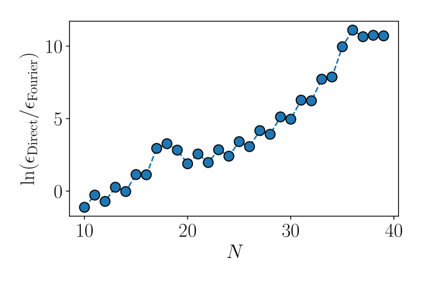
Figure 1: Logarithm of the relative accuracy $\epsilon_{\rm direct}/\epsilon_{\rm Fourier}$ of the discretized direct formula [Eq. (13)] with respect to the discretized Fourier formula [Eq. (20)], for a fixed number of grid points $N$. Note that the relative error increases exponentially with $N$.

We set the stage by reviewing and comparing the Fourier options pricing method with vanilla Monte Carlo for the European call option under geometric Brownian motion. These results are already well established but serve as a baseline for extension to the multi-asset case. In the single asset case, we compare the convergence of the Monte Carlo algorithm in the number of samples to the Fourier method [Eq. (20)] and the direct method [Eq. (13)] in the number of interpolation points. Figure 1 shows the relative accuracy $\epsilon_{\rm direct}/\epsilon_{\rm Fourier}$ with $\epsilon_{\kappa}=\frac{|V_{\kappa}-V_{\rm exact}|}{V_{\rm exact}}$, and $\kappa=\{{\rm direct},{\rm Fourier}\}$. For the same number of grid points, the Fourier method dramatically outperforms the direct integration. While the direct integration converges with an inverse polynomial, the Fourier method converges faster than polynomially and likely exponentially in the number of integration points. For the Fourier options simulation, we use $\eta=0.5$ and $\alpha=3$ as fixed hyperparameters. The two kinks in the data are artefacts of the method. They depend on the choice of $\eta$. If $\eta$ is too large, the kinks become more pronounced, but the exponential scaling in $N$ levels off before reaching computer precision limits. The parity of $N$ also plays a role in the accuracy of the Fourier method. For further analysis of the Fourier method on a single asset, see Ref. [21] and references therein.

In this experiment, the vanilla Monte Carlo approach reaches a standard deviation of $10^{-4}$ for $10^{10}$ — $10^{11}$ samples, which is impractical on a laptop. For comparison, the direct integration requires $N\geq 100$ grid points, and the Fourier method requires only $N\geq 30$ grid points, both running in milliseconds on a laptop. Therefore, the Fourier methods provides remarkable speedup over the other two methods in the single asset case. We now demonstrate that this advantage can be extended to the multi-asset case by using the tensor network approach outlined above.

V.2 The multi-asset case

In the multi-asset case, we consider the minimum payoff [Eq. (11)] and a parametrized family of correlated geometric Brownian motion with correlation matrix:

$$\Sigma(\beta)=(\beta|+\rangle\langle+|+\mathbbm{1})/(1+\beta),$$ (31)

where we restrict $0\leq\beta\leq 1$. Here, the state $|+\rangle=\sum_{j=1}^{d}|j\rangle$, and the correlation matrix has $\beta/(1+\beta)$ on the off diagonals, and ones on the diagonal. This choice of covariance matrix, although artificial, captures with a single parameter the amount of correlation in the dynamics of the problem. Our general conclusions extend to other correlated dynamics. We set the number of grid points to $N=50$, which guarantees an accuracy well within $10^{-4}$. The imaginary shift is chosen to be $\alpha=5/d$, which satisfies the requirements ${\rm Im}[z_{j}]>0$ and $\sum_{j=1}^{d}{\rm Im}[z_{j}]>1$, and allows for good stability of the TT-cross algorithm while guaranteeing rapid convergence.

Table 1: Runtime and accuracy results for a single typical run of the tensor-Fourier algorithm on the min-option for multi-asset geometric Brownian motion with a covariance matrix given in Eq. (31) with $\beta=0.5$. $t_{\rm wall}$ is the wall clock time, $t_{\rm rel}$ is the ratio of the wall clock time for the tensor-Fourier method over vanilla Monte Carlo, $r_{\rm comp}$ is the compression ratio of the computation, $\epsilon_{\rm trunc}$ is the MPS truncation error compared with the full tensor, $D_{w}$ and $D_{\varphi}$ are the bond dimensions of the two MPS, and $\eta$ is the grid spacing in momentum space.

$d$	$t_{\rm wall}$[s]	$t_{\rm rel}$	$r_{\rm comp}$	$\epsilon_{\rm trunc}$	$D_{v}$	$D_{\varphi}$	$\eta$
$2$	$0.027$	$3\times 10^{-5}$	$3.6$	$1.42\times 10^{-6}$	$20$	$10$	$0.5$
$3$	$0.73$	$5.4\times 10^{-4}$	$1.056$	$4.10\times 10^{-6}$	$20$	$10$	$0.4$
$4$	$6.8$	$0.0038$	$0.074$	$1.84\times 10^{-6}$	$30$	$15$	$0.3$
$5$	$10.2$	$0.0045$	$0.0022$	—	$30$	$15$	$0.3$
$6$	$13.7$	$0.0051$	$5.85\times 10^{-5}$	—	$30$	$15$	$0.2$
$7$	$52.8$	$0.017$	$2.58\times 10^{-6}$	—	$40$	$20$	$0.2$
$8$	$63.4$	$0.018$	$6.19\times 10^{-8}$	—	$40$	$20$	$0.2$
$9$	$74.0$	$0.018$	$1.44\times 10^{-9}$	—	$40$	$20$	$0.2$
$10$	$84.5$	$0.019$	$3.30\times 10^{-11}$	—	$40$	$20$	$0.2$
$15$	$326.8$	$0.048$	$2.67\times 10^{-19}$	—	$50$	$25$	$0.2$

We simulate the correlated multi-asset option with the tensor Fourier algorithm based on the TT-cross algorithm described in Sec. IV, the correlated multi-asset option with the full summation of Eq. (24) up to $d=4$, and the correlated multi-asset option with a vanilla Monte Carlo simulation (Sec. III.1). A typical single shot run is reported in Table 1. $D_{v}$ is the bond dimension used in TT-cross algorithm for the MPS approximation of $|\hat{v}\rangle$, and $D_{\varphi}$ is the bond dimension used in the TT-cross algorithm for the MPS approximation of $|\varphi_{T}\rangle$. Both are chosen so as to guarantee convergence of TT-cross algorithm in a single sweep with convergence tolerance $\epsilon_{\rm tol}=0.005$. We find empirically that allowing for several sweeps does not improve the convergence significantly, nor does progressively increasing the bond dimension at each sweep. $t_{\rm wall}$ is the wall clock time in seconds for the tensor-Fourier algorithm. $r_{\rm comp}$ is the compression ratio, defined as the number of oracular function calls made by the TT-cross algorithm divided by the total grid size $N^{d}$. The truncation error $\epsilon_{\rm trunc}$ is defined as the ratio between the options price calculated in the MPS approximation generated via the TT-cross algorithm and the full tensor. The comparison already becomes infeasible for $d=5$ without further compression tricks. The relative time $t_{\rm rel}$ is defined as the ratio of wall clock time for the tensor Fourier method over the wall clock time for vanilla Monte Carlo with $n=5\times 10^{7}$ samples, which guarantees precision up to $10^{-3}$. With $50$ grid points and the hyperparameters indicated in the table, we expect the tensor-Fourier results to reach a precision well within $10^{-4}$. Hence, the $t_{\rm rel}$ speedup is a conservative estimate. The wall clock time for Monte Carlo is calculated on the same hardware as the tensor-Fourier simulations for $d=2$. For $d>2$, the Monte Carlo wall clock time is extrapolated assuming a linear scaling with the dimension $d$. This estimate is also conservative, because the Monte Carlo simulations scale slightly super-linearly. The comparison with Monte Carlo is meant to give an indication of the ballpark computational time for the tensor-Fourier method. A much more detailed analysis would be required to compare an optimal Monte Carlo method, such as multilevel Monte Carlo [3], to an optimal tensor-Fourier method, using perhaps the COS transform [31]. Furthermore, the relative advantages of different methods depends strongly on the application at hand. Our interest is in showing the feasibility and potential advantages of the tensor-Fourier method.

The wall clock time $t_{\rm wall}$ depends sensitively on $D_{v}$ and $D_{\varphi}$, and only weakly on $d$. The runtime of the TT-cross algorithm is expected to scale as ${\mathcal{O}}(dND^{2})$ [13]. Still, the runtime is modest up to large dimensionality, maintaining several order of magnitude speedup over the vanilla Monte Carlo approach. The compression ratio $r_{\rm trunc}$ gives an idea of how efficiently the MPS can be constructed via the TT-cross algorithm. The number of oracular calls to the integrand scales as ${\mathcal{O}}(ND^{2})$. The truncation error $\epsilon_{\rm trunc}$ does not appear to depend sensitively on $d$. Rather, it is determined by the choice of convergence criterion of the TT-cross algorithm.

Ultimately, the strength of the Fourier approaches is the ability to reach extremely high precision in a reasonable time. Our numerical results indicate that this is the case up to at least $d=15$ assets. We find that beyond $d=15$, the TT-cross algorithm has trouble converging. This is likely caused by a proliferation of local minima and rugged optimization landscapes. It is an interesting open research question, whether there are good schemes for providing the TT-cross algorithm with a warm start for larger systems or to embed it into a meta-heuristic to overcome the ruggedness of the landscape.

V.3 The bond dimension

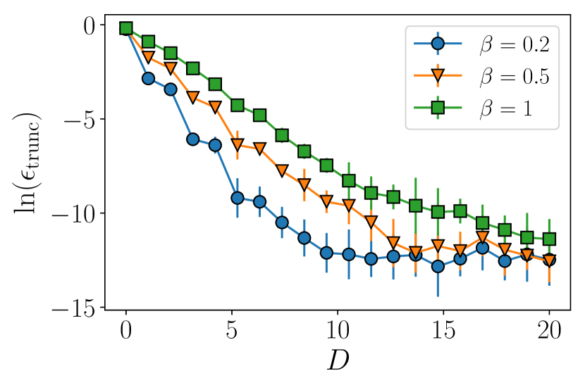
Figure 2: Logarithm of the truncation error as a function of the bond dimension $D_{\varphi}$ for $\beta=0.2$, $0.5$,$1$, and $d=3$.

The wall clock time, the compression ratio and the truncation error all depend sensitively on the choice of bond dimensions. We discuss how how the bond dimension of the MPS for the characteristic function $|\varphi_{T}\rangle$ and the payoff function $|\hat{v}_{\rm min}\rangle$ depends on the various hyperparameters of the system.

The tensor network solver relies heavily on the TT-cross subroutine which is heuristic and involves stochastic components. In particular, the random staring point for the TT-cross algorithm affects the convergence significantly. What we observe in our experiments is that, when the bond dimension is sufficiently large (although not too large), the TT-cross algorithm reliably converges. When the bond dimension is taken too small, TT-cross algorithm does not converge. In the intermediate regime, the starting point is essential to guarantee convergence. However, we notice that the quality of the approximation can be reasonably good even though TT-cross algorithm does not converge. This is not inconsistent, because the convergence criterion reflects the actual proximity of the original vectors and their MPS approximation, while we are interested in functionals of the vectors.

This can be seen in Fig. 2 where the convergence to non-convergence transition happens for $D\approx 10\beta$ for a convergence criterion of $\epsilon=0.005$, but the error in the approximation of the function decreases exponentially in $D$. This suggests that our algorithm smoothly improves with $D$. Figure 2 also shows the logarithm of the truncation error for a $d=3$ experiment for different intensities of correlations. The reported results are averaged over $20$ runs. The bond dimension for $|\hat{v}_{\rm min}\rangle$ is taken to be $D_{v}=30$ to guarantee an accurate representation of the tensor. Hence all of the inaccuracy is caused by the MPS truncation error of the characteristic function $|\varphi_{T}\rangle$.

We consistently observe that the accuracy improves exponentially with the bond dimension $D_{\varphi}$, with an exponent inversely proportional to $\beta$. The precision saturates at a level close to $\log(\epsilon_{\rm trunc})=-12$. We do not know what causes the saturation, but we expect that is has to do with TT-cross algorithm reaching local minima when the bond dimension is taken to be large.

VI Discussion

We have shown how to use tensor network methods to extend the applicability of Fourier options pricing to the many asset setting. This promises to dramatically reduce the computational time of multi-asset options pricing, in a similar way as is already the case for single asset options. The natural question remains as to when the tensor network approach is applicable. There are two natural extensions to be considered for practical applications. First, to adapt the method to more complex multi-asset instruments and second, to adapt it to different forms of stochastic dynamics.

The forms of stochastic dynamics that naturally fit into our framework are those for which the (multivariate) characteristic function is known analytically. This includes, among others, the Merten jump model [17] and the Heston stochastic volatility model [18]; two of the most commonly used models in options pricing. Other models such as the SABR model [15] do not have a know analytic form of the characteristic function, but there exist methods to extend Fourier options pricing to them. More complex multi-asset instruments could be challenging to generalise, yet we already know how to extend some common ones such as basket and rainbow options [32]. Time-dependent options can also be treated following ideas taken from Ref. [33]. Therefore, the tensor Fourier approach holds the promise of accelerating many common multi-asset derivatives pricing models. How great the speedup is will ultimately depend on the nature and complexity of the given instrument.

- [1] John C Hull. Options futures and other derivatives. Pearson Prentice Hall, Upper Saddle River, NJ, 2006.
- [2] Peter A Acworth, Mark Broadie, and Paul Glasserman. A comparison of some monte carlo and quasi monte carlo techniques for option pricing. In Monte Carlo and Quasi-Monte Carlo Methods 1996, pages 1–18. Springer, 1998.
- [3] Michael B Giles. Multilevel monte carlo methods. Acta Numerica, 24:259–328, 2015.
- [4] Lina von Sydow, Lars Josef Höök, Elisabeth Larsson, Erik Lindström, Slobodan Milovanović, Jonas Persson, Victor Shcherbakov, Yuri Shpolyanskiy, Samuel Sirén, Jari Toivanen, et al. Benchop–the benchmarking project in option pricing. International Journal of Computer Mathematics, 92(12):2361–2379, 2015.
- [5] Nikitas Stamatopoulos, Daniel J Egger, Yue Sun, Christa Zoufal, Raban Iten, Ning Shen, and Stefan Woerner. Option pricing using quantum computers. Quantum, 4:291, 2020.
- [6] Patrick Rebentrost, Brajesh Gupt, and Thomas R Bromley. Quantum computational finance: Monte carlo pricing of financial derivatives. Physical Review A, 98(2):022321, 2018.
- [7] Shouvanik Chakrabarti, Rajiv Krishnakumar, Guglielmo Mazzola, Nikitas Stamatopoulos, Stefan Woerner, and William J Zeng. A threshold for quantum advantage in derivative pricing. Quantum, 5:463, 2021.
- [8] Javier Gonzalez-Conde, Ángel Rodríguez-Rozas, Enrique Solano, and Mikel Sanz. Pricing financial derivatives with exponential quantum speedup. arXiv preprint arXiv:2101.04023, 2021.
- [9] Koichi Miyamoto. Bermudan option pricing by quantum amplitude estimation and chebyshev interpolation. arXiv preprint arXiv:2108.09014, 2021.
- [10] Ashley Montanaro. Quantum speedup of monte carlo methods. Proceedings of the Royal Society A: Mathematical, Physical and Engineering Sciences, 471(2181):20150301, 2015.
- [11] Andrew M Childs, Jin-Peng Liu, and Aaron Ostrander. High-precision quantum algorithms for partial differential equations. Quantum, 5:574, 2021.
- [12] Ashley Montanaro and Sam Pallister. Quantum algorithms and the finite element method. Physical Review A, 93(3):032324, 2016.
- [13] Ivan Oseledets and Eugene Tyrtyshnikov. Tt-cross approximation for multidimensional arrays. Linear Algebra and its Applications, 432(1):70–88, 2010.
- [14] Fischer Black and Myron Scholes. The pricing of options and corporate liabilities. The Journal of Political Economy, 81(3):637–654, 1973.
- [15] Patrick S Hagan, Deep Kumar, Andrew S Lesniewski, and Diana E Woodward. Managing smile risk. The Best of Wilmott, 1:249–296, 2002.
- [16] Hélyette Geman and Marc Yor. Pricing and hedging double-barrier options: A probabilistic approach. Mathematical finance, 6(4):365–378, 1996.
- [17] Alan L Lewis. A simple option formula for general jump-diffusion and other exponential lévy processes. Available at SSRN 282110, 2001.
- [18] Steven L Heston. A closed-form solution for options with stochastic volatility with applications to bond and currency options. The review of financial studies, 6(2):327–343, 1993.
- [19] Zaza van der Have and Cornelis W Oosterlee. The cos method for option valuation under the sabr dynamics. International Journal of Computer Mathematics, 95(2):444–464, 2018.
- [20] Peter Carr and Dilip Madan. Towards a theory of volatility trading. Option Pricing, Interest Rates and Risk Management, Handbooks in Mathematical Finance, pages 458–476, 2001.
- [21] Martin Schmelzle. Option pricing formulae using fourier transform: Theory and application. Preprint, http://pfadintegral. com, 2010.
- [22] Ernst Eberlein, Kathrin Glau, and Antonis Papapantoleon. Analysis of fourier transform valuation formulas and applications. Applied Mathematical Finance, 17(3):211–240, 2010.
- [23] Ivan V Oseledets. Tensor-train decomposition. SIAM Journal on Scientific Computing, 33(5):2295–2317, 2011.
- [24] Lev I Vysotsky, Alexander V Smirnov, and Eugene E Tyrtyshnikov. Tensor-train numerical integration of multivariate functions with singularities. arXiv preprint arXiv:2103.12129, 2021.
- [25] Sergey Dolgov and Dmitry Savostyanov. Parallel cross interpolation for high-precision calculation of high-dimensional integrals. Computer Physics Communications, 246:106869, 2020.
- [26] Qingquan Song, Hancheng Ge, James Caverlee, and Xia Hu. Tensor completion algorithms in big data analytics. ACM Transactions on Knowledge Discovery from Data (TKDD), 13(1):1–48, 2019.
- [27] Ulrich Schollwöck. The density-matrix renormalization group in the age of matrix product states. Annals of physics, 326(1):96–192, 2011.
- [28] Garnet Kin-Lic Chan and Sandeep Sharma. The density matrix renormalization group in quantum chemistry. Annual review of physical chemistry, 62:465–481, 2011.
- [29] Sergei A Goreinov and Eugene E Tyrtyshnikov. The maximal-volume concept in approximation by low-rank matrices. Contemporary Mathematics, 280:47–52, 2001.
- [30] https://github.com/vmml/tntorch.
- [31] Fang Fang and Cornelis W Oosterlee. A novel pricing method for european options based on fourier-cosine series expansions. SIAM Journal on Scientific Computing, 31(2):826–848, 2009.
- [32] Ruggero Caldana, Gianluca Fusai, Alessandro Gnoatto, and Martino Grasselli. General closed-form basket option pricing bounds. Quantitative Finance, 16(4):535–554, 2016.
- [33] Fang Fang and Cornelis W Oosterlee. A fourier-based valuation method for bermudan and barrier options under heston’s model. SIAM Journal on Financial Mathematics, 2(1):439–463, 2011.