From Empirical Observations to Universality:
Dynamics of Deep Learning with Inputs Built on Gaussian mixture
Abstract
This study broadens the scope of theoretical frameworks in deep learning by delving into the dynamics of neural networks with inputs that demonstrate the structural characteristics to Gaussian Mixture (GM). We analyzed how the dynamics of neural networks under GM-structured inputs diverge from the predictions of conventional theories based on simple Gaussian structures. A revelation of our work is the observed convergence of neural network dynamics towards conventional theory even with standardized GM inputs, highlighting an unexpected universality. We found that standardization, especially in conjunction with certain nonlinear functions, plays a critical role in this phenomena. Consequently, despite the complex and varied nature of GM distributions, we demonstrate that neural networks exhibit asymptotic behaviors in line with predictions under simple Gaussian frameworks.
I Introduction
The endeavor to connect practical deep learning applications with theoretical understanding is a growing field of research [1, 2, 3, 4, 5]. Recent studies in this area have begun to study on neural network characteristics under structured nature of input data [6, 7, 8, 9, 10, 11, 12].
The notion of structured data posits that despite the high-dimensional nature of typical datasets (such as MNIST in LeCun [13] has 28x28, CIFAR in Saad and Solla [14] has 3x32x32), these can often be distilled into lower-dimensional representations. This concept is exemplified in the MNIST dataset, where digits, rather than being random pixel assemblies, exhibit structured patterns like lines and circles. This phenomenon of low-dimensional structural features in data has been corroborated by numerous studies [15, 16, 17, 18, 19, 20].
From discussions on the presence of these low-dimensional structural features, considerable research has delved into the intriguing aspects manifested in deep learning when inputs with such characteristics are presented. Particularly, recent studies have found that when inputs inherently exhibit single Gaussian distribution traits, these characteristics are preserved even after passing through the first layer, facilitating a theoretical understanding of deep learning dynamics in simple two-layer models [9, 10, 11].
However, these significant theoretical discoveries fall short of fully mirroring the complexities and heterogeneities of real-world data. Typically, Gaussian mixtures are preferred over single Gaussian distributions for modeling general data characteristics [21, 22, 23], with recent findings suggesting that real-world data often follows Gaussian mixture-like distributions [24, 12]. This gap underscores the necessity for our investigation into Gaussian mixture-based models to capture the complexity of real-world data more accurately. Given this context, our research extends the current theoretical discourse by examining the neural network dynamics when inputs are characterized not by simple Gaussian but by Gaussian mixtures. More specifically, we analyze how neural network dynamics changes as the inherent distribution deviate from simple Gaussian to Gaussian mixture.
Our main findings from investigation into neural network dynamics reflecting Gaussian mixture structural properties are follow:
-
•
Applying “standardization” to input datasets with inherent Gaussian mixture properties reveals convergence to the predicted dynamics outcomes of existing theories [10].
-
•
This observed non-divergence is attributed to the distinctive characteristics of nonlinear functions utilized in deep learning network and dataset modeling process, makes deep learning dynamics are predominantly influenced by the distribution’s lower-order cumulants.
The subsequent section, Background II, will present a concise overview of the relevant research. The Methods section III will introduce the Gaussian mixture settings employed in our research and explain the methodology developed to analyze the deviation in dynamics as the distribution changes from a simple Gaussian to a Gaussian mixture. In the Results section IV, we delineate a sequence of experiments showcasing intriguing patterns of convergence, even when the distribution markedly deviates from the typical simple Gaussian distribution. In the Discussion section V, we present a mathematical proof that clarifies the observed phenomena.
II Background
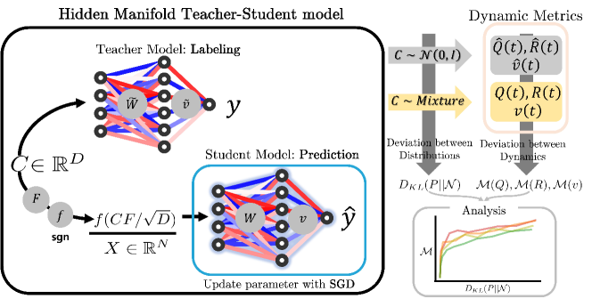
This section offers a overview of the teacher-student model framework and introduces its evolved variant, the Hidden Manifold Teacher-Student model, as proposed by Goldt et al. [10]. We explain how preceding research efforts have approached the task of understanding theoretical dynamics within the manifold model context.
II.1 Hidden Manifold Teacher-Student Model
The teacher-student model is well-regarded method in the study of high-dimensional problems [25, 26, 4, 5]. This model framework consists of a teacher model, which generates dataset labels, and a student model that learns these labels. Our study specifically zeroes in on the dynamics of a fully-connected two-layer neural network.
The weights of the first and second layers of the teacher model are represented by matrices and , respectively. We define the activation function of the teacher model as . Similarly, the weights of the first and second layers of the student model are denoted by and , with the activation function represented as .
In the canonical teacher-student model, the input is typically an element-wise i.i.d. from a Gaussian distribution.
However, our desired input characteristics are not inherently Gaussian but should reflect intrinsic properties as seen in datasets like the Swiss-roll, which exists on a specific manifold.
To embed these intrinsic properties into the input , they utilize a -dimensional vector that follows an element-wise i.i.d. Gaussian distribution. This is achieved through a feature matrix and a nonlinear function as follows:
| (1) |
By modeling the dataset in this manner, the input intrinsically follows the characteristics of which is distributed as a Gaussian. Furthermore, the labels generated by the teacher model are derived not directly from , but from , which reflects intrinsic characteristics. In essence, the teacher model generates labels, and the student model learns these labels as follows:
| (2) |
This model, recognizing a hidden structure in lower dimensions, is termed the Hidden Manifold Teacher-Student model [10].
Additionally, for the convenience of subsequent discussions, let’s denote the preactivations of the teacher and student models as and , respectively:
| (3) |
When input spans beyond a singular data point to represent a dataset of size , it assumes a matrix form, denoted as . Consequently, each preactivation is expressed through matrices and .
The notation will represent the element located at the -th row and -th column of any given matrix , and will denote the -th component of any vector .
Furthermore, in the theoretical analysis to follow, we frequently consider the limit where the dataset dimensions and intrinsic dimension become infinitely large (), a scenario often referred to as the thermodynamic limit from the perspective of statistical physics. To maintain consistency with prior theoretical studies, this research also adopts the term thermodynamic limit to describe the scenario.
II.2 Dynamics of Neural Network are dominant by correlation of function
In this study, we update weights through a simple scaled stochastic gradient descent (SGD) with a batch size of one, under quadratic loss :
To illustrate a straightforward example, let’s examine the dynamics through the explicit ordinary differential equation (ODE) form of the second weight, . Defining the normalized number of steps as in the thermodynamic limit , which can be interpreted as a continuous time-like variable. Consequently, satisfies the following ODE.
| (4) |
where and represent the correlations of function.
Using a similar approach for , we can derive the dynamics of our teacher-student model in the form of ODEs, as detailed in the Appendix B. The dynamics are predominantly influenced by the correlations of specific functions, like . To calculate these function correlation values, we requires information on the underlying distribution of .
II.3 The Gaussian Equivalence Property
Previous analyses have delved into understanding the distribution of preactivations under certain assumptions. To summarize the findings, adhere to a Gaussian distribution characterized by a specific covariance matrix.
To provide a simplified derivation, we first explore how the function correlation approximately follows. Suppose random variables from a joint Gaussian distribution are weakly correlated (), and arbitrary functions are regular enough to guarantee the existence of an expectation value, then the following lemma holds:
Lemma II.1 (Function correlation approximation).
| (5) |
If the feature matrix and the student weight matrix are sufficiently bounded, fulfilling the following assumption:
Assumption II.2 (Bounded assumption).
For all and any indices :
| (6) |
we can approximately calculate the covariances of , i.e., . By referring to the definition of and employing the lemma II.1 to decompose each function correlation, and then sorting out the terms that vanish in the thermodynamic limit () according to the bounded assumption (Appendix A.3).
This analysis enables the derivation of the asymptotic form of all covariance matrices, where higher-order correlation vanish in the thermodynamic limit [10]. Consequently, the preactivations follow a Gaussian distribution, a result summarized as the Gaussian Equivalence Property (GEP).
Property II.3 (Gaussian Equivalence Property (GEP)).
In the thermodynamic limit (, ), with finite , , , and under the assumption II.2, if the follows a normal Gaussian distribution , then conform to jointly Gaussian variables. This means that statistics involving are entirely represented by their mean and covariance.
Just as the dynamics of significantly depend on the distribution characteristics of , the neural network’s dynamics can be analyzed through these distribution characteristics (Appendix B). This property II.3 allows for an understanding of the student and teacher models’ dynamics, via the mean and covariance of the joint Gaussian distribution of preactivations. A comprehensive derivation and discussion are provided in the appendix A and B.
For convenience, let’s redefine as:
| (7) |
also follows a jointly Gaussian distribution, and its expectation value satisfies .
Consequently, the new distribution follows a more straightforward distribution with the mean
| (8) |
and the covariance
| (9) | ||||
| (10) | ||||
| (11) |
Here, , , and represent the statistical properties of the nonlinear function , used in the transformation of student model inputs , ,
| (12) |
under . The newly defined matrices satisfy the following relations:
| (13) | ||||
| (14) | ||||
| (15) |
These defined covariances capture essential characteristics inherent to the teacher-student model dynamics. Given that the weights of the student model, and , evolve under the stochastic gradient descent (SGD) dynamics, these values, and consequently the covariances , , , inherently depend on the progression of training steps (time).
The student model learns by attempting to emulate the teacher model’s outputs. Each covariance matrix holds a distinct significance in relation to the dynamics of the model. Specifically, signifies the correlation between the preactivations of the student and teacher models, reflecting the student model’s accuracy in mirroring the teacher. Conversely, relates to the correlation among the student model’s own preactivations, implying the dynamics of the student model’s first layer. While remains constant throughout the learning process and thus stands apart from and , it serves as a mirror to the teacher model’s inherent characteristics.
To summarize, within the context of a hidden manifold teacher-student model characterized by simple Gaussian distribution properties, the learning dynamics of the student model are primarily influenced by terms like . Such terms, which depend on the distributional properties of , can be calculated once distribution determined. Under certain assumptions, the GEP elucidates that the preactivations follow a Gaussian distribution. Consequently, this allows us to analytically dissect the dynamics of the student model.
III Method
In this section, we detail our approach to configuring Gaussian mixture inputs and explain the methodology developed to analyze the shift in dynamics as the distribution changes from a simple Gaussian to a Gaussian mixture. Our study’s dynamic metrics of interest are , , and .
III.1 Gaussian mixture setting
In this study, instead of the simple Gaussian input () used in previous research, we employ a more generalized Gaussian mixture distribution as the input of teacher model . Here, we describe the Gaussian mixture setting utilized in our analysis. Consider a random variable emerging from a -dimensional Gaussian mixture with mixture components. can be represented as:
where the sum of the probabilities .
To gauge the divergence of our Gaussian mixture from a standard Gaussian distribution, we utilize the Kullback–Leibler (KL) divergence as the metric for distribution distance. The KL divergence quantifies the statistical discrepancy between two distributions, defined for the divergence of from as:
| (16) |
For our Gaussian mixture’s components, we fix the deviation for all and assign the means by uniformly distributing them within the interval . Hence, a random variable from Gaussian mixture distribution comprising Gaussian components is formalized as follows:
| (17) |
For convenience, we denote this specific Gaussian mixture distribution as .
By defining the Gaussian mixture model in this manner, we ascertain that increasing leads to a monotonically increasing KL divergence from a single Gaussian (Appendix D).
This methodology allows us to undertake empirical investigations across a spectrum of Gaussian mixtures by adjusting the parameters and .
III.2 Analyzing Discrepancies in Dynamics: Gaussian to Gaussian Mixture Inputs
This section explains the methods to explore how neural network dynamics deviates as input () originally assumed Gaussian, transitions towards a Gaussian mixture. Our examination centers around metrics such as , , and the second-layer weight of the student model. While the generalization error is undoubtedly a critical feature, the behavior of error decreasing is a common characteristic under trainable datasets, distinguishing it slightly from , , and .
The methodology initiates with the assignment of initial values to the weights () and the feature matrix . Firstly, with drawn from a Gaussian mixture distribution , we obtain , and at each step of the training process via SGD.
Subsequently, using identical initial values () and the feature matrix , we obtain , , and through ODEs based on theoretical analysis (Appendix B). This is theoretically equivalent to the dynamics observed with SGD when originates from a simple Gaussian distribution .
Theoretical ODE results (, , ) and empirical SGD results (, , ) are collected at each time step.
Given that both sets of dynamics commence from identical starting conditions, significant discrepancies are not initially observed. To evaluate the extent of divergence in network dynamics, we employ the temporal Log-sampled Root Mean Squared Error (tLog-RMSE, ) as our metric. We temporally log-sampled both ODE results and SGD results then computed the Root Mean Squared Error (RMSE) for these sampled data points. For instance, the tLog-RMSE for and can be formulated as follows:
| (18) |
where represents the log-sampled time points derived from the original time steps.
Furthermore, we examine two distinct scenarios concerning the teacher model’s input : standardization and un-standardization.
In the unstandardized scenario, is directly utilized from the distribution . Conversely, the standardized scenario implements a simple standardization method, where the random variable is rescaled as
| (19) |
The expectation value is computed by empirical samples, . For the sake of clarity and convenience in notation, we refer to the standardized setting as .
III.3 Additional Detailed Experimental Conditions
In this study, the dimension was set to and the dimension for student input to . The dimensions of the hidden layers for both teacher and student models were uniformly set to . For the activation functions, both the teacher and student models utilized the same function, or ReLU function. The nonlinear function was employed to generate the student input. The learning rate was set at , and training was conducted using the quadratic loss . The SGD update used was a single batch SGD with layerwise learning rate scaling, as mentioned earlier II.2. For training, the neural network was updated for a total of steps.
IV Results
In this section, we delve into the empirical exploration of how the dynamics shift as the input distribution transitions from a simple Gaussian to a Gaussian mixture. Through our investigation, we evaluated 20 distinct Gaussian mixtures, each undergoing training steps. Since SGD dynamics are influenced by randomness and ODE dynamics can fluctuate by numerical errors, it is possible for the results of SGD in the simple Gaussian setting to differ from those of the ODE results, that should theoretically be identical. Out of the 20 different Gaussian mixtures, excluding those where the ODE results and the SGD dynamics of the simple Gaussian significantly different, we sampled 10 for analysis.
The results provided the average tLog-RMSE value across these varied mixtures. The dimensions of matrices and vectors are , and .
For instance, since the dynamic metric consists of a total of four values (), the average tLog-RMSE value is calculated as follows:
| (20) |
As defined above, for convenience of notation, the absence of an index indicates the average, while the explicit presence of an index refers to the tLog-RMSE value for that specific index.
We calculate the KL divergence , across different that parametrized by as mixture setting outlined earlier (17). It then assessed the influence of these values on the discrepancies, tLog-RMSE.
Note the spectrum of KL divergence varies across different components, depending on . In our Gaussian mixture setting, since the components have mean values , an increase in the number of components can lead to overlapping phenomena, thereby reducing the KL divergence. This effect can be observed in subsequent results, where slightly different lengths along the KL divergence axis are shown.
In the main text, our emphasis is on the results obtained using the ReLU activation function. For outcomes related to the erf activation function, refer to Appendix G.
IV.1 Results from un-standardized Gaussian mixture
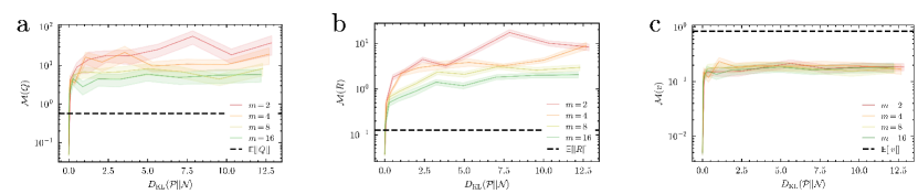
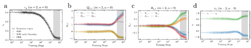
As observed in Figure 2, the dynamics under un-standardized Gaussian mixture settings significantly diverge from those under a simple Gaussian distribution. Analyzing various mixture settings, we investigate the relationship between KL divergence and the error metric .
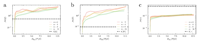
Figure 3 intriguingly demonstrates that despite significant deviation from (increasing KL divergence), certain dynamic metrics— and —tend to converge towards an asymptotic limit. This results simply explained by non-divergence (or non-explosive) nature of our learning dynamics. Despite the Gaussian mixture deviating significantly from a simple Gaussian distribution, the student’s trainable parameters do not explode. As a result, the non-divergence property guarantees that the error in the dynamics metric does not exhibit exponential behavior.
IV.2 Results from standardized Gaussian mixture
Subsequently, we investigated the dynamics under teacher model inputs , derived from the standardization of Gaussian mixture samples.
Interestingly, the dynamics under standardized Gaussian mixture settings closely resemble those under a simple Gaussian distribution. In Figure 4, this similarity is readily apparent.
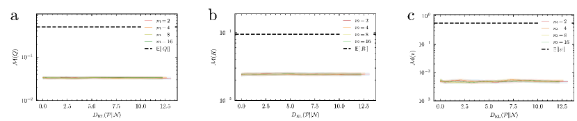
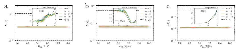
The analysis of dynamics with standardized Gaussian mixtures yielded notably insightful outcomes. As illustrated in Figure 5, the average tLog-RMSE for various mixtures appears minimal relative to the metrics’ scale, indicated by a dotted line. These mixtures do not introduce any significant discrepancies between theoretical predictions and empirical observations. The subsequent Discussion section V will provide explanation of these phenomena, why mixture based experiment result conceptually converge with conventional theory.
V Discussion
In this section, we delve into the mathematical analysis of the convergence properties of the standardized Gaussian mixture.
As discussed in the Background section II, the dynamics of our teacher-student model setting are influenced by the distribution followed by . Therefore, to analyze how network dynamics change when is a Gaussian mixture, it is crucial to examine the distribution of under such a mixture setting.
Following the proof sequence for the Gaussian Equivalence Property II.3 where adhere to a Gaussian distribution, we first investigate how the expectation of function correlations converges in the context of a Gaussian mixture, then derive a modified version of GEP applicable to this scenario.
V.1 Convergence in Standardized Gaussian Mixtures
V.1.1 Correlations between Functions with Gaussian mixture
Consider random variables represented as and . Each variable and originates from a Gaussian mixture: with probability where , and similarly, with probability where .
Despite utilizing Gaussian mixtures, each random variable can essentially be considered as following a single Gaussian distribution with a certain probability, allowing us to straightforwardly implement the existing function correlation approximation II.1. In the Gaussian mixture setting, we derive the following lemma for function correlation approximation under mixture distribution:
Lemma V.1 (Function correlation approximation with mixture distribution).
For the case with two Gaussian mixture variables and standardized to mean zero and variance one, and assuming weakly correlated covariance (, , ), the approximation of function correlation for the Gaussian mixture in the limit as is given by:
| (21) |
with
Therefore, even with Gaussian mixtures, an approximation of function correlation can achieve a similar form.
V.1.2 Dominance of Moments in the Expectation Value of Functions
In deriving the original Gaussian Equivalence Property II.3 we utilized the approximation form of function correlation II.1 to determine the covariance matrix of . Since the Lemma V.1 has equivalent form with Lemma II.1, remaining question pertains to how the expectation values of functions ( or ) under random variables , following a Gaussian mixture distribution, differ from those assuming random variables following simple Gaussian distribution.
In our study, we particularly employed the sgn function as our function within the . Dissecting the sgn function into differentiable regions reveals that higher-order derivative terms become negligible. This insight, coupled with Taylor expansion, allows us to probe the characteristics of the expectation value for a random variable following an arbitrary distribution.
For simplicity, we introduce the following notation:
Definition V.2.
Given an arbitrary distribution denoted by and another distribution denoted by , if shares identical cumulants with up to order 2, we represent as , .
Under this setting, for specific functions where higher-order differential terms are insignificant, the following lemma is derived:
Lemma V.3 (Function Expectation Approximation).
Let be a random variable with mean and variance under distribution . Suppose is a function almost everywhere (), with the condition that for or , 1. , and 2. for is negligible in the certain limit of our interest. Then, function expectation possesses the following approximate property:
The derivation hinges on the function ’s property, which erase the effect of high-order related terms, leading to convergence to the same expectation value. Detailed derivation can be found in the appendix C.
This suggests that for any random variable standardized to mean zero and variance one, the expected value of its function, , can be closely approximated by .
Thus, for a standardized Gaussian mixture distribution , since the nonlinear function satisfies the condition, the expectations of covariance components in the Gaussian mixture align closely with their Gaussian counterparts:
| (22) | |||
| (23) | |||
| (24) |
The summary of above convergence can summarized under Modified Equivalence Property:
Property V.4 (Modified Equivalence Property).
With the same condition of II.3 except and the distribution of is standardized Gaussian mixture , take the Gaussian Equivalence Property’s results distribution as . Then the under standardized Gaussian mixture random variable , current preactivation distribution follows such that
| (25) |
It is important to note that is not follow Gaussian distribution but only shares identical cumulants with up to order 2.
Surprisingly, if the neural network’s activation function , also satisfy the condition for function expectation approximation V.3, results to their correlation with the random variables , such as , used in the ODE formulation of , also exhibits an approximated equivalence.
Fortunately, where the ReLU serves as the activation function, its piecewise second derivative is inherently zero. The higher order term in Taylor expansion is less dominant then the lower order term. Thus, a loose approximation is viable:
| (26) |
Thus, even without higher order equivalence between and , the core dynamics governing the neural network exhibit approximate equivalence.
In summary, our findings articulate the following points:
- 1.
-
2.
Specific functions that meet the criteria outlined, predominantly influence the function expectation by the first and second cumulants, V.3.
-
3.
This adaptation and the conditions specified lead to an equivalence in the covariance of preactivations , achieve equivalence up to second cumulants from a distribution perspective, V.4.
- 4.
If erf were used as the activation function, since function is bounded , the conditions for lemma V.3 would have been satisfied more loosely, and a similar discussion could be applicable.
Ultimately, despite the input distributions deviating from a Gaussian form, within the thermodynamic limit (, ) and for specific functions that adhere to the conditions of lemma V.3—where the expectation value is dominated by the first and second moments—the dynamics of neural networks asymptotically converge to those anticipated under simple Gaussian inputs. This convergence facilitates the incorporation of dynamics observed under Gaussian mixtures into conventional theoretical frameworks originally devised for single Gaussian inputs.
This broadens the applicability of these theories, extending their relevance to encompass scenarios not previously considered in analyses confined to simple Gaussian inputs, thereby enhancing our theoretical understanding of neural networks across a more diverse array of input distributions.
VI Conclusion
Previous research has extensively explored the dynamics under a hidden manifold with a simple Gaussian distribution [9, 10, 11], as well as under Gaussian mixtures in the absence of a hidden manifold [27, 28]. Our study represents a expansion of previous works, aiming to broaden the scope of understanding. We delved into investigating dynamics neural network when exposed to Gaussian mixtures in manifold—a more comprehensive representation of distributions. We scrutinized the discrepancies between dynamics under simple Gaussian based input and dynamics under Gaussian mixture based input with SGD update rule, yielding insightful findings.
The key takeaway from our investigation is the pivotal role of standardization. Applying standardization to Gaussian mixtures facilitates an alignment with the predictions posited by pre-existing conventional theories [10]. Furthermore, our rigorous mathematical substantiation enabled the extension of these conventional theories to accommodate a broader spectrum of distributions. This results underscores that, notwithstanding variations in the input structure from a Gaussian baseline, the dynamics of the student model essentially adhere to conventional theoretical models.
In essence, our study unveils a newfound universality in which the inferences drawn from function correlation and the Gaussian Equivalence Property retain their validity within the domain of Gaussian mixtures. Given the generalized Gaussian mixture model assumption and its substantial expressive capacity, it stands to reason that a similar universality might be observed across other distributions. Moreover, our mathematical justification, predicated on the significance of the first and second moments (V.3, V.4), paves the way for extending this framework to encompass a more diverse array of distributions, both traditional and beyond.
The inherent structural properties of data offer an intriguing and insightful foundation for exploration. By incorporating these characteristics into the analysis of deep learning dynamics, we aim to bridge the gap between the impressive practical successes of applied deep learning and the still-emerging theoretical research. Ultimately, we hope our research seeks to deepen the understanding of deep learning, contributing to further breakthroughs and insights in the field.
VII Reproducibility
For a comprehensive understanding of our numerical SGD implementation and ODE update mechanisms, along with ensuring reproducibility, please visit our code repository at the following link: https://github.com/peardragon/_GaussianMixture.
Acknowledgements.
This study was supported by the Basic Science Research Program through the National Research Foundation of Korea (NRF Grant No. 2022R1A2B5B02001752).References
- Seung et al. [1992] H. S. Seung, H. Sompolinsky, and N. Tishby, Physical review A 45, 6056 (1992).
- Engel [2001] A. Engel, Statistical mechanics of learning (Cambridge University Press, 2001).
- Zdeborová and Krzakala [2016] L. Zdeborová and F. Krzakala, Advances in Physics 65, 453 (2016).
- Bahri et al. [2020] Y. Bahri, J. Kadmon, J. Pennington, S. S. Schoenholz, J. Sohl-Dickstein, and S. Ganguli, Annual Review of Condensed Matter Physics 11, 501 (2020).
- Zdeborová [2020] L. Zdeborová, Nature Physics 16, 602 (2020).
- Bartlett et al. [2020] P. L. Bartlett, P. M. Long, G. Lugosi, and A. Tsigler, Proceedings of the National Academy of Sciences 117, 30063 (2020).
- Korada and Montanari [2011] S. B. Korada and A. Montanari, IEEE transactions on information theory 57, 2440 (2011).
- Candès and Sur [2020] E. J. Candès and P. Sur, The Annals of Statistics 48, 27 (2020).
- Goldt et al. [2019] S. Goldt, M. Advani, A. M. Saxe, F. Krzakala, and L. Zdeborová, Advances in neural information processing systems 32 (2019).
- Goldt et al. [2020] S. Goldt, M. Mézard, F. Krzakala, and L. Zdeborová, Physical Review X 10, 041044 (2020).
- Goldt et al. [2022] S. Goldt, B. Loureiro, G. Reeves, F. Krzakala, M. Mézard, and L. Zdeborová, in Mathematical and Scientific Machine Learning (PMLR, 2022) pp. 426–471.
- Dandi et al. [2023] Y. Dandi, L. Stephan, F. Krzakala, B. Loureiro, and L. Zdeborová, arXiv preprint arXiv:2302.08933 (2023).
- LeCun [1998] Y. LeCun, http://yann. lecun. com/exdb/mnist/ (1998).
- Saad and Solla [1995] D. Saad and S. A. Solla, Physical Review Letters 74, 4337 (1995).
- Pope et al. [2021] P. Pope, C. Zhu, A. Abdelkader, M. Goldblum, and T. Goldstein, arXiv preprint arXiv:2104.08894 (2021).
- Fefferman et al. [2016] C. Fefferman, S. Mitter, and H. Narayanan, Journal of the American Mathematical Society 29, 983 (2016).
- Hinton and Salakhutdinov [2006] G. E. Hinton and R. R. Salakhutdinov, science 313, 504 (2006).
- Peyré [2009] G. Peyré, Computer vision and image understanding 113, 249 (2009).
- Creswell et al. [2018] A. Creswell, T. White, V. Dumoulin, K. Arulkumaran, B. Sengupta, and A. A. Bharath, IEEE signal processing magazine 35, 53 (2018).
- Goodfellow et al. [2020] I. Goodfellow, J. Pouget-Abadie, M. Mirza, B. Xu, D. Warde-Farley, S. Ozair, A. Courville, and Y. Bengio, Communications of the ACM 63, 139 (2020).
- Carreira-Perpinan [2000] M. A. Carreira-Perpinan, IEEE Transactions on Pattern Analysis and Machine Intelligence 22, 1318 (2000).
- Scott [2015] D. W. Scott, Multivariate density estimation: theory, practice, and visualization (John Wiley & Sons, 2015).
- Goodfellow et al. [2016] I. Goodfellow, Y. Bengio, and A. Courville, Deep Learning (MIT Press, 2016) http://www.deeplearningbook.org.
- Seddik et al. [2020] M. E. A. Seddik, C. Louart, M. Tamaazousti, and R. Couillet, in International Conference on Machine Learning (PMLR, 2020) pp. 8573–8582.
- Gabrié [2020] M. Gabrié, Journal of Physics A: Mathematical and Theoretical 53, 223002 (2020).
- Baity-Jesi et al. [2018] M. Baity-Jesi, L. Sagun, M. Geiger, S. Spigler, G. B. Arous, C. Cammarota, Y. LeCun, M. Wyart, and G. Biroli, in International Conference on Machine Learning (PMLR, 2018) pp. 314–323.
- Refinetti et al. [2021] M. Refinetti, S. Goldt, F. Krzakala, and L. Zdeborova, in Proceedings of the 38th International Conference on Machine Learning, Proceedings of Machine Learning Research, Vol. 139, edited by M. Meila and T. Zhang (PMLR, 2021) pp. 8936–8947.
- Loureiro et al. [2021] B. Loureiro, G. Sicuro, C. Gerbelot, A. Pacco, F. Krzakala, and L. Zdeborová, Advances in Neural Information Processing Systems 34, 10144 (2021).
- Marchenko and Pastur [1967] V. A. Marchenko and L. A. Pastur, Matematicheskii Sbornik 114, 507 (1967).
Appendix: From Empirical Observations to Universality:
Dynamics of Deep Learning with Inputs Built on Gaussian mixture
A Derivation of Gaussian Equivalent Property
0.1 Correlation of Two Functions
It is important to consider how to express the correlation of functions, such as , for the analysis of neural network dynamics. Let’s consider random variables following a distribution and examine the correlation of functions taking these random variables as inputs.
Represent two random variables, adhering to a Joint Gaussian Distribution, as vectors,
| (S1) |
The assumption of joint Gaussian distribution for these random variables implies that the vectors have the following mean and covariance.
| (S2) |
The joint distribution of and can be represented as:
| (S3) |
Considering a first-order approximation in , the inverse matrix part becomes,
| (S4) |
Inserting this back into the joint distribution and approximating again with respect to , we obtain following results.
| (S5) | ||||
To directly apply the aforementioned equation to the correlation of two functions, consider and as functions of and , respectively. Provided these functions are sufficiently regular to possess expectations , , , and , the correlation between the two functions can be expressed as:
| (S6) |
0.2 Gaussian Equivalence Property
From the function correlation approximations, it becomes clear that for functions of sufficient regularity, their correlations are primarily dictated by the function’s mean, distribution characteristics such as , and the covariance of the original random variables. This underscores the pivotal role of function correlation in dissecting the dynamics within neural networks.
In our investigation, the weight update mechanism is facilitated by employing a straightforward stochastic gradient descent (SGD) strategy, with the batch size set to one.
| (S7) | ||||
| (S8) |
By defining the normalized number of steps as within the thermodynamic limit as , which analogously functions as a continuous time-like variable, we are equipped to elucidate the dynamics of the second layer weight in the student model by examining the function correlations of the preactivations from an averaged standpoint. Consequently, the dynamics of adhere to the following ODE formulation.
| (S9) |
Given the crucial role of function correlation in unpacking the dynamics prompted by weight updates, it is imperative to understand the distribution characterizing to compute expectation values such as . This analytical approach enables a deeper understanding of the underlying mechanics governing the behavior of neural networks, particularly in how weight adjustments influence overall learning and adaptation processes.
Unlike the earlier discussion on simple function correlation, where the variable of the function was assumed to be a simple Gaussian, in the context of deep learning SGD updates, the random variable entering the function is not just an assumable random variable but the preactivations.
Therefore, it’s essential to ascertain the distribution of these preactivations. Let’s make the following assumptions:
Assumption A.1.
In the thermodynamic limit , , matrices , , and possess explicit bounds:
| (S10) |
Assumption A.2.
Even when considering matrices and together, they maintain explicit bounds. For all and any indices :
| (S11) |
In typical deep learning scenarios, activations that address gradient vanishing or explosiveness involve gradients directly influencing weight updates in a non-vanishing limit. Thus, considering bounds for student weights during initialization is sufficient. Since the remaining teacher weights and feature matrix are constant, ensuring proper bounds for teacher and student weights during initialization, and setting the feature matrix to be sufficiently bounded, these assumptions can be adequately met.
With these assumptions and the result of function correlation, the Gaussian Equivalence Property holds as follows:
Property A.3 (Gaussian Equivalence Property (GEP)).
This property allows us to representing characteristics of the student and teacher models, generalization error and dynamics of the student model’s second layer weights, through the mean and covariance of the joint Gaussian distribution of preactivations.
For convenience, let’s redefine as:
| (S12) |
also follows a jointly Gaussian distribution, and its expectation value satisfies as per function correlation.
In this appendix, we present a concise derivation of . For a additional derivation, we refer the reader to prior research [9]. To facilitate the explanation, we first define , , and as statistical properties of the nonlinear function , which is utilized in transforming the student model inputs , where :
| (S13) |
With these definitions in place, can be expressed as follows:
| (S14) | ||||
| (S15) |
Considering the case where , and applying the expectation, we implement the function correlation approximation S6 to derive:
| (S16) | ||||
| (S17) | ||||
| (S18) |
Hence, can be succinctly rearranged for both and cases as:
| (S19) | ||||
| (S20) |
A similar approach can be applied to derive the remaining covariance components. Regarding high-order moments, an analogous method is employed by extending the function correlation approximation S6 to more general cases, thereby demonstrating that such preactivations follow a Gaussian distribution in the thermodynamic limit. For a comprehensive explanation of this process, the reader is encouraged to consult the referenced research [9].
Consequently, the new distribution follows a more straightforward distribution with the mean
| (S21) |
and the covariance
| (S22) | ||||
| (S23) | ||||
| (S24) |
The newly defined matrices satisfy the following relations:
| (S25) | ||||
| (S26) | ||||
| (S27) |
B Derivation of the ODE for Covariance and Weights
To derive the ODE for our main metrics of interest - the covariances , , and the 2nd layer weight - we begin with our single batch gradient update.
| (S28) | ||||
| (S29) |
The preactivations are related to the first layer weights, and thus we consider quantities such as and that are proportional to the first layer weights . The dynamics of the first layer weights are determined by a term involving , assuming the second layer is constant. The average update of these quantities can be obtained from the following equation:
| (S30) |
Starting with , we obtain:
| (S31) |
with .
Function correlations are employed to express these updates in terms of statistical quantities of the distributions . However, the equations for covariances remain coupled. To uncouple them, we need to consider the eigenvectors and eigenvalues, and , of the matrix formed by . The eigenvectors and eigenvalues are obtained under the following normalization condition:
| (S32) |
Using these, we can express the teacher-student overlap covariance through two projected matrices:
| (S33) |
and thus:
| (S34) |
Since the teacher model’s matrix is static, its projection matrix is given by:
| (S35) |
The update rule for is then derived using these projections. Explicitly at timestep , it can be expressed as:
| (S36) |
During the summation over , two types of terms emerge:
| (S37) |
The second summation is not readily reducible to a simpler expression. Instead, we introduce the following density function:
| (S38) |
This density function allows us to express the covariance in terms of the eigenvalue distribution :
| (S39) |
Under the assumption that the feature matrix elements are i.i.d. from a normal distribution , this distribution adheres to the Marchenko-Pastur law [29]:
| (S40) |
The update equation for is straightforwardly derived from the update equation and definition of . Ultimately, in the thermodynamic limit, with transforming into a continuous time-like variable, the equation of motion for satisfies the following ODE:
| (S41) | ||||
where . Note that all explicit time dependencies on the right side of the equation are omitted for clarity. In this numerical ODE implementation, the right side corresponds to the immediate preceding time , and the left side to the updated time .
Similarly, the covariance associated with the first weight can be derived in a repetitive manner, starting from:
| (S42) |
Following a similar process as before, we find that the first term, , adheres to:
| (S43) | ||||
The second term, , can be expressed using the rotating basis :
| (S44) |
and thus, integral form for can be derived:
| (S45) |
with
| (S46) | ||||
The weight and generalization error can be directly obtained from the weight update formula and the definition of generalization error with MSE:
| (S47) |
with
| (S48) | ||||
C Derivation of Function Expectation Approximation Lemma
Lemma’s statement is as following:
Lemma C.1.
Let be a random variable with mean and variance under distribution . Suppose is a function almost everywhere (), with the condition that for or , 1. , and 2. for is negligible in the certain limit of our interest. Then, function expectation possesses the following approximate property:
To derive above lemma, First, to use Taylor expansion, we need to separate the interval. And since the condition of approaches yield follwing results.
Let’s take part. Since the lemma condition making vanishing of high order derivation, we can directly found expectation of the function approximately converges to the expectation under distribution.
Applying a similar approach to other terms leads to the general result that the expectation value of a function over a random variable from a distribution can be approximated by the expectation value of the same function over a random variable from a standard Gaussian distribution :
Functions like erf, ReLU, and sgn approximately satisfy the aforementioned condition, allowing for the following equivalency in expectation values.
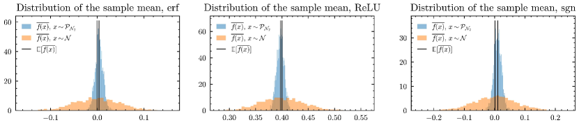
The distribution of the sample mean follows a Gaussian distribution under the limit of a large number of samples, . Under this, we can empirically verify the lemma results for erf, ReLU, and sgn. The Figure S1 shows approximately the same expectation of sample mean .
D KL divergence under Gaussian Mixture setting
Experimentally, by adjusting the distribution bound of the mixture component means , we observed a regular correlation in the KL divergence between the mixture distribution and the normal Gaussian distribution [Figure S1].
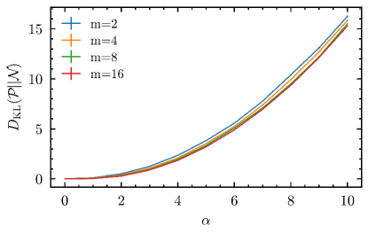
This approach enabled us to conduct empirical analyses on various Gaussian mixtures by adjusting the values of and .
E Additional Detailed Experimental Conditions
In this study, the dimension was set to and the dimension for student input to . The dimensions of the hidden layers for both teacher and student models were uniformly set to . For the activation functions, both the teacher and student models utilized the same function, or ReLU function. The nonlinear function was employed to generate the student input. The learning rate was set at , and training was conducted using the Mean Squared Error (MSE) loss, . The SGD update used was a single batch SGD with layerwise learning rate scaling, as mentioned earlier II.2. For training, the neural network was updated for a total of steps.
For more detailed information on the numerical SGD implementation and ODE update implementation, please refer to the following code repository: https://github.com/peardragon/_GaussianMixture. Our research was carried out on a computing setup equipped with an AMD Ryzen 7 7700X CPU and an NVIDIA GeForce RTX 3060 12GB GPU.
F Detailed tLog-RMSE Results
In the main text, we utilized the average tLog-RMSE for the sake of conciseness and clarity in presenting our results. However, to provide additional detail, this section provides the average values of each dynamics metric and their corresponding tLog-RMSE values.
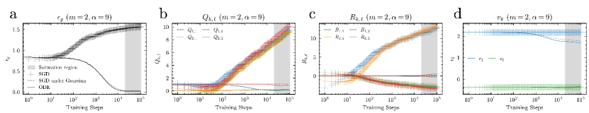
The definitions inherent to each dynamics metric suggest that for , off-diagonal terms are expected to be less correlated, whereas for , it is the diagonal terms that are anticipated to exhibit less correlation.
This expectation is shown in our results, where metrics indicative of less correlation elements demonstrated lower values.
The observations shared in the main body of the text, the number of components impacts are negligible under the standardization setting. Herein, we focus specifically on the case where , presenting the outcomes in a tabular format. Each value has been rounded to three decimal places .
| 0.090 | 0.040 | 0.035 | 0.093 | 0.030 | 0.036 | 0.036 | 0.032 | 0.012 | 0.014 | |
| 0.083 | 0.044 | 0.039 | 0.092 | 0.028 | 0.036 | 0.036 | 0.032 | 0.012 | 0.013 | |
| 0.091 | 0.044 | 0.037 | 0.092 | 0.028 | 0.036 | 0.036 | 0.032 | 0.013 | 0.015 | |
| 0.086 | 0.044 | 0.039 | 0.095 | 0.028 | 0.035 | 0.037 | 0.032 | 0.012 | 0.014 | |
| 0.091 | 0.041 | 0.037 | 0.094 | 0.028 | 0.038 | 0.037 | 0.033 | 0.013 | 0.014 | |
| 0.085 | 0.042 | 0.037 | 0.088 | 0.028 | 0.037 | 0.036 | 0.031 | 0.013 | 0.014 | |
| 0.083 | 0.043 | 0.036 | 0.096 | 0.027 | 0.034 | 0.036 | 0.032 | 0.012 | 0.014 | |
| 0.088 | 0.044 | 0.040 | 0.092 | 0.027 | 0.036 | 0.037 | 0.032 | 0.013 | 0.014 | |
| 0.090 | 0.042 | 0.037 | 0.094 | 0.029 | 0.036 | 0.037 | 0.032 | 0.012 | 0.014 | |
| 0.083 | 0.041 | 0.037 | 0.089 | 0.029 | 0.035 | 0.036 | 0.030 | 0.013 | 0.015 | |
| 0.995 | 0.093 | 0.093 | 0.988 | 0.088 | 0.126 | 0.129 | 0.085 | 0.488 | 0.508 |
| 0.037 | 0.036 | 0.038 | 0.041 | 0.024 | 0.024 | 0.026 | 0.028 | 0.006 | 0.006 | |
| 0.037 | 0.035 | 0.038 | 0.041 | 0.024 | 0.025 | 0.027 | 0.027 | 0.007 | 0.006 | |
| 0.036 | 0.036 | 0.038 | 0.039 | 0.025 | 0.025 | 0.026 | 0.028 | 0.006 | 0.006 | |
| 0.035 | 0.035 | 0.039 | 0.040 | 0.025 | 0.025 | 0.027 | 0.028 | 0.008 | 0.006 | |
| 0.037 | 0.036 | 0.037 | 0.044 | 0.025 | 0.025 | 0.026 | 0.031 | 0.006 | 0.006 | |
| 0.037 | 0.037 | 0.037 | 0.041 | 0.025 | 0.026 | 0.027 | 0.028 | 0.006 | 0.007 | |
| 0.035 | 0.036 | 0.037 | 0.042 | 0.025 | 0.024 | 0.027 | 0.028 | 0.006 | 0.006 | |
| 0.037 | 0.035 | 0.038 | 0.041 | 0.025 | 0.026 | 0.027 | 0.028 | 0.007 | 0.007 | |
| 0.037 | 0.036 | 0.038 | 0.039 | 0.025 | 0.024 | 0.026 | 0.027 | 0.006 | 0.006 | |
| 0.036 | 0.033 | 0.040 | 0.038 | 0.026 | 0.025 | 0.026 | 0.028 | 0.006 | 0.006 | |
| 0.847 | 0.053 | 0.064 | 1.009 | 0.053 | 0.089 | 0.072 | 0.165 | 0.507 | 0.597 |
G Results under erf activation function
Similar results can be observed even when using the error function (erf) as the activation function.