Tomography of flavoured leptogenesis with primordial blue gravitational waves

Abstract

We explore a scenario where an early epoch of matter domination is driven by the mass scale $M_{N}$ of the right-handed neutrinos, which also characterizes the different flavour regimes of leptogenesis. Such a matter-domination epoch gives rise to peculiar spectral imprints on primordial Gravitational Waves (GWs) produced during inflation. We point out that the characteristic spectral features are detectable in multiple frequency bands with current and future GW experiments in case of Blue GWs (BGWs) described by a power-law with a positive spectral index $(n_{T}>0)$ and an amplitude compatible with Cosmic Microwave Background (CMB) measurements. We find that the three-flavour leptogenesis regime with $M_{N}\lesssim 10^{9}~{}{\rm GeV}$ imprints BGWs more prominently than the two-flavour and one-flavour regimes characterized by a higher right-neutrino mass scale. In particular, a two-flavour (three-flavour) leptogenesis regime is expected to leave distinct imprints in the mHz ($\mu$Hz) band. Moreover, we translate the current Big Bang Nucleosynthesis (BBN) and LIGO limits on the GW energy density into constraints on the flavour leptogenesis parameter space for different GW spectral index $n_{T}$. Interestingly, a three-flavour leptogenesis regime can offer a unique signal testable in the next LIGO run with a correlated signature in the PTA frequency band with an amplitude comparable to the one expected from supermassive black holes.

I introduction

Primordial Gravitational Waves (GWs) can be a unique probe of physics operating at super high-energy scales that are otherwise unreachable, e.g., with terrestrial accelerators. Broadly, a high-energy theory/model can be sensitive to GWs in two ways. First, the model can accommodate a source of GWs whose amplitude and spectral features relate to the model parameters. Thus, the model becomes testable with the GW searches. On the other hand, the model can leave its imprints on GWs, regardless of how they are produced. This article discusses the latter case. Let us assume a spectrum of primordial GWs, which might be of inflationary origin [1, 2], and we aim at probing a post-inflation high-energy model with those GWs . In a given scenario where the underlying dynamics of GWs production are known, we expect specific spectral features in the GWs today. Therefore, testing an independent model (which is not related to the origin of GWs) would require finding detectable imprints in those GWs caused exclusively by the model under consideration. This method proposed as a tomographic search of BSM theories with GWs [3, 4] is similar to X-ray tomography of an object, wherein the object is placed in front of an X-ray source, and we let the X-ray pass through the object to know the invisible internal properties of the object. Likewise, the GW tomography has two main ingredients: the source, specifically the GW spectrum, and the object, namely the high-energy model to be tested.

In this article, for GW spectrum, we consider primordial Blue Gravitational Waves (BGWs) with $\Omega_{\rm GW}\sim f^{n_{T}}$ (here $\Omega_{\rm GW}$ is the GWs energy density, $f$ is the frequency and $n_{T}>0$ is a spectral index) which might come, e.g., from inflation. For the high-energy model we want to probe, we consider thermal leptogenesis, which is a process that generates the baryon asymmetry of the universe [5]. BGWs are appealing by several considerations. First, for $n_{T}>0$, the BGWs come with strong amplitude, and therefore, they are easily detectable, given the projected sensitivities of the current and planned GW detectors operating at different frequency bands. Second, the recent finding of nHz stochastic GWs by the Pulsar Timing Arrays (PTAs) shows a strong preference for a blue-tilted GW spectrum of primordial origin [6, 7, 8, 9, 10, 11, 12, 13, 14, 15, 16]. Specifically, a power-law fit to the 15 yrs NANOGrav PTA data renders a large spectral index value; $n_{T}\sim 1.2-2.4$ at $68\%$ CL [10]. Third, because of their potentially strong amplitude in the sub-nHz and $\mu$Hz regions, primordial BGWs are among the very few candidates that can be tested with Pulsar parameter drifts [17, 18] and possibly with Lunar Laser Ranging (LLR) [19, 20]. Finally, as recently pointed out, BGWs might affect large-scale structures by sourcing density perturbations at second order [21]. Although we shall not provide any model that might produce such BGWs, let us mention that the simplest single-field slow-roll inflation models produce a nearly scale-invariant spectrum with very small amplitude. Nonetheless, plenty of scenarios [22, 23, 24, 25, 26, 27, 28, 29, 30, 31] go beyond the simplest one and predict BGWs that are detectable.

Leptogenesis [5] is a two-step process: a lepton asymmetry is created in the first step, which is then processed to a baryon asymmetry via the sphaleron transition [32]. Among several possibilities to generate lepton asymmetry [33, 34, 35], here we consider the one within the seesaw framework of light neutrino masses. In this scenario, CP-violating and out-of-equilibrium decays of right-handed (RH) neutrinos to lepton and Higgs doublet produce lepton asymmetry. Typically, at a temperature $T\sim M_{N}$, where $M_{N}$ is the RH neutrino mass scale, lepton asymmetry gets produced. Depending on the several variants, a wide range of RH neutrino mass window, $M_{N}\in[\rm MeV,10^{15}\rm GeV]$ [36, 37, 38, 39, 40, 41, 42, 43, 44, 45], might facilitate a successful leptogenesis. As it is obvious, $M_{N}\gtrsim\mathcal{O}(\rm TeV)$ scales are not reachable with collider experiments, and so leptogenesis operating on those scales requires alternative probes. A way to test such a high-scale scenario is provided by the flavour effects [46, 47, 48] which connect it indirectly to low-energy neutrino observables, specifically to the leptonic CP violation [49]. A flavoured leptogenesis scenario can have three distinct regimes (as described in the next section): one-flavour/vanilla regime (1FL) for $M_{N}\gtrsim 10^{12}$ GeV, two-flavour regime (2FL) for $10^{12}$ GeV $\gtrsim M_{N}\gtrsim 10^{9}$ GeV, and three-flavour regime (3FL) for $M_{N}\lesssim 10^{9}$ GeV. Though connecting those regimes with low-energy neutrino observables is possible, it is difficult to differentiate them observationally because of plenty of free parameters in seesaw models. One way to distinguish them is to impose further symmetries in the Lagrangian, e.g., discrete symmetries, to reduce the number of parameters [50, 51]. Here, we shall show that, alternatively, with the GW-tomography method, not only can such high scales be probed, but different flavour regimes can potentially leave distinct imprints on the BGW spectrum.

As outlined, given an independent source of GWs, testing a model requires finding imprints on the GW spectrum caused by the model. Therefore, probing different mass scales of leptogenesis (hence different flavour regimes) requires finding characteristic GW spectral features dependent on RH masses. We show that, though nontrivial, this can be done within some parameter space in the seesaw models, which offers an RH neutrino mass-dependent matter epoch affecting the standard propagation (in radiation domination) of primordial BGWs. The idea is based on contemplating the origin of RH neutrino masses. Let us suppose that, like any other Standard Model (SM) particles, the RH neutrinos get their mass via a phase transition triggered by an SM singlet scalar field. Once the field rolls down to its vacuum and attains its vacuum expectation value, besides generating RH neutrino masses, it oscillates coherently around the vacuum. Such oscillations persist long with a null equation of state parameter (the field behaves like matter) when the scalar field lives longer. A probable timeline in the scenario has been illustrated in Fig. 1. Suppose the coupling of the scalar field to the RH neutrino plays a pivotal role in determining its lifetime. In that case, the duration of the matter domination can be controlled by the coupling and, therefore, by the RH neutrino masses. This is the key aspect of our study. Irrespective of their origin, as primordial gravitational waves pass through such a matter-dominated phase, the beginning and the end of the matter-dominated phase get imprinted on the final GW spectrum. Therefore, the final GW spectrum carries imprints of the RH neutrino mass scale.

Within a concrete model of $U(1)_{B-L}$ phase transition triggered by a scalar field $\Phi$ carrying $B-L$ charge, the key feature of our study is that a peaked BGW spectrum gets distorted when it passes through such an RH neutrino mass-dependent matter epoch and finally exhibits a double-peaked spectrum when the scalar field lives longer. The locations of the low-frequency peak ($f_{\rm low}^{\rm peak}$) and the dip ($f^{\rm dip}$) in between are strongly sensitive to RH neutrino masses. As the leptogenesis process enters from an unflavoured to flavour regimes, these two characteristic frequencies shift from a high to a low-frequency value, and the ratio $\Omega_{\rm GW}(f_{\rm low}^{\rm peak})/\Omega_{\rm GW}(f_{\rm dip})$ increases. While the vanilla leptogenesis scenario hardly imprints the GW spectrum, the two-flavour and the three-flavour regimes exhibit characteristic spectral features in the GWs in the mHz and $\mu$Hz bands. The scenario can accommodate a reasonably large value of $n_{T}$ without contradicting any cosmological constraints and allows the overall spectrum to span a wide range of frequencies accessible to the current and planned GW detectors. Notably, in the PTA frequency band, flavoured leptogenesis regimes allow GW amplitude comparable to supermassive black hole binaries (SMBHB).

The rest of the paper is organized as follows. In Sec. II, we discuss the scalar field dynamics and all the constraints the model must comply with. In Sec. III, we present a detailed numerical study on how the BGW spectrum contains information on the RH neutrino mass scale. We also discuss our model in the context of the recent PTA results on nHz GWs. Finally, we draw our conclusions in Sec. IV.

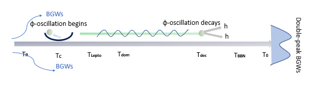
Figure 1: A schematic timeline showing the occurrence of the events considered in this work. After inflation, the universe reheats at $T=T_{\rm R}$. Phase transition happens, the scalar field oscillation begins, and RH neutrinos become massive at $T=T_{c}$. At the temperature $T_{\rm lepto}\simeq M_{N}$, the baryon asymmetry produced by the RH neutrinos freezes out. Starting from $T_{\rm dom}$ until $T_{\rm dec}$, the scalar field dominates the universe’s energy density and produces entropy around $T\simeq T_{\rm dec}$. The universe becomes radiation-dominated after this. The big-bang nucleosynthesis and the current temperature are denoted by $T_{\rm BBN}$ and $T_{0}$, respectively. A peaked blue-tilted GW-spectrum generated during inflation when comes across such a dynamical phase of $\Phi$, which also makes the RH neutrino massive and whose decay width is determined by the RH neutrino mass scale, becomes a double peak spectrum at present. The final spectrum carries imprints of the RH neutrino mass scale and, therefore, different regimes of leptogenesis.

II scalar field dynamics and the scale of thermal Leptogenesis

The Lagrangian relevant to the discussion is given by

$$-\Delta\mathcal{L}\subset f_{Di\alpha}\overline{N_{Ri}}\tilde{H}^{\dagger}L_{\alpha}+\frac{1}{2}f_{Ni}\overline{N_{Ri}}\Phi N_{Ri}^{C}+\frac{1}{4}\lambda_{H\Phi}|H|^{2}|\Phi|^{2}+V(\Phi,T)\,,$$ (II.1)

where $f_{D}$ is the neutrino Dirac Yukawa coupling, $H(L)$ is the SM Higgs (lepton doublet), $N_{R}$ is the RH neutrino field, $\Phi$ is a complex scalar field with vacuum expectation value $v_{\Phi}$, and $V(\Phi,T)$ is the finite temperature potential that determines the phase transition dynamics of $\Phi$. Here, $N_{R}$ and $L$ have $B-L$ charge $-1$, whereas the same charges for $\Phi$ and $H$ are $2$ and $0$, respectively. The Higgs portal coupling is in general given by $\lambda_{H\Phi}\simeq\lambda_{H\Phi}^{\rm tree}+\lambda_{H\Phi}^{\rm 1-loop}$ where $\lambda_{H\Phi}^{\rm 1-loop}$ is generated by the first two terms in Eq. (II.1). We assume $\lambda_{H\Phi}^{\rm tree}=0$ which is crucial to establish a connection between the neutrino parameters and the lifetime of $\Phi$. The RH neutrinos become massive ($M_{i}=f_{Ni}v_{\Phi}$) when $\Phi$ obtains its vacuum expectation value $v_{\Phi}$. After the electroweak phase transition ($T\lesssim T_{\rm EW}$), when the Higgs settles to its minima $H=v_{h}$, the first two terms generate light active neutrino mass $m_{\nu i}\sim{f_{Di}}^{2}v_{h}^{2}/M_{i}$ via the standard type-I seesaw mechanism [57, 58, 59, 60], whereas at $T\gg T_{\rm EW}$ the heavy neutrinos decay CP asymmetrically to lepton doublets plus Higgs, and generate lepton asymmetry. At a temperature $T\sim M_{i}$, lepton asymmetry produced by $i$th RH neutrino freezes out; therefore, $M_{i}$ is typically the scale of thermal leptogenesis. For the sake of simplicity, not focusing so much on the hierarchy in $M_{i}$s, we consider a single scale for the rest of the discussion, i.e. $M_{i}\equiv M_{N}=f_{N}v_{\Phi}$. In the high-scale leptogenesis scenario, there are three distinct regimes of leptogenesis [46, 47, 48]. Generally, the RH neutrinos produce lepton doublets as a coherent superposition of flavours: $\ket{L_{i}}=A_{i\alpha}\ket{L_{\alpha}}$, where $\alpha=e,\mu,\tau$ and $A_{i\alpha}$ is the corresponding amplitude determined by $f_{Di\alpha}$. For temperatures $T\gtrsim 10^{12}~{}{\rm GeV}$, all the charged lepton Yukawa couplings are out of equilibrium (the interaction strength is given by $\Gamma_{\alpha}\sim 5\times 10^{-3}~{}f_{L\alpha}T$, with $f_{L\alpha}$ being the charged lepton Yukawa coupling) and do not participate in the leptogenesis process. This is the unflavour or the vanilla regime of leptogenesis. In this regime, leptogenesis is not sensitive to the neutrino mixing matrix, e.g. mixing angles and low-energy CP phases. When the temperature drops down to $T\lesssim 10^{12}~{}{\rm GeV}$, the $\tau$ flavoured charged lepton interaction comes into equilibrium and breaks the coherent $\ket{L_{i}}$ state into $\tau$ and a composition of $e+\mu$ flavour (two flavour regime). Likewise, the later composition is broken once $T\lesssim 10^{9}~{}{\rm GeV}$, when the $\mu$ flavoured charged lepton interaction comes into equilibrium (three flavour regime). In both these flavoured regimes, leptogenesis may be sensitive to the low-energy neutrino parameters. We will explore all these regimes and show that the flavoured regime of leptogenesis leaves much more distinct imprints on BGWs than the vanilla one, paving the path for a possible synergy between low-energy neutrino physics and GWs.

As the temperature drops, the scalar field transits from $\Phi=0$ towards its vacuum expectation value $\Phi=v_{\Phi}$. The finite temperature potential that restores the symmetry at higher temperatures is given by [61, 62, 63, 64, 65]

$$V(\Phi,T)=D(T^{2}-T_{0}^{2})\Phi^{2}-ET\Phi^{3}+\frac{\lambda}{4}\Phi^{4}\,,$$ (II.2)

with

$$D=\frac{3{g^{\prime}}^{2}+4\lambda}{24}\,,~{}~{}E=\frac{3{g^{\prime}}^{3}+{g^{\prime}}\lambda+3\lambda^{3/2}}{24\pi}\,,~{}~{}T_{0}=\frac{\sqrt{12\lambda}v_{\Phi}}{\sqrt{3{g^{\prime}}^{2}+4\lambda}}\,,$$ (II.3)

where $g^{\prime}$ is the gauge coupling, and the vacuum expectation value $v_{\Phi}=\mu/\sqrt{\lambda}$ has been determined from the zero temperature potential $V(\Phi,0)=-\frac{\mu^{2}}{2}\Phi^{2}+\frac{\lambda}{4}\Phi^{4}$. The structure of the finite temperature potential determines how the transition proceeds. The last term in Eq. (II.2) generates a potential barrier causing a secondary minimum at $\Phi\neq 0$, which at $T=T_{c}$ becomes degenerate with the $\Phi=0$ one. At $T_{0}~{}(\lesssim T_{c})$, the potential barrier vanishes, making the minimum at $\Phi=0$ a maximum [63]. The critical temperature $T_{c}$ and the field value $\Phi_{c}=\Phi\left(T_{c}\right)$ are given by [63, 66]

$$T_{c}=T_{0}\frac{\sqrt{\lambda D}}{\sqrt{\lambda D-E^{2}}}\,,~{}~{}\Phi_{c}=\sqrt{\frac{4D}{\lambda}(T_{c}^{2}-T_{0}^{2})}\,.$$ (II.4)

A non-zero value of $E$ in Eq. (II.2) generally leads to a first-order transition with a strength determined roughly by the order parameter $\Phi_{c}/T_{c}$ [63]. Nonetheless, if $\Phi_{c}/T_{c}\ll 1$, the transition is weakly first-order, which can be treated as a second-order transition because the potential barrier disappears quickly. In this case, the transition can be described by rolling of the field $\Phi$ from $\Phi=0$ to $\Phi=v_{\Phi}$. In this article, we consider such a case working with the values of $\lambda$ and ${g^{\prime}}$ so that $\Phi_{c}/T_{c}\ll 1$ is fulfilled. In particular, we find that, for ${g^{\prime}}^{3}\lesssim\lambda\lesssim 1$ and ${g^{\prime}}\lesssim 10^{-2}$, the order parameter is $\Phi_{c}/T_{c}\lesssim 0.08$. Fixing the hierarchy between the couplings to be $\lambda\simeq{g^{\prime}}^{3}$ (limiting condition), we also have $T_{c}\simeq T_{0}=2\sqrt{g^{\prime}}v_{\Phi}$.

Once the field rolls down to the true vacuum, it oscillates around $v_{\Phi}$. For a generic potential $V(\Phi)=\alpha\Phi^{\beta}$, the equation of state of such a coherent oscillation can be computed as [3]

$$\omega=(\beta-2)(\beta+2)^{-1}\,.$$ (II.5)

Assuming the oscillation of the scalar field is driven by the dominant quadratic term in the potential and expanding the zero temperature potential around the true vacuum, we obtain $\alpha=\lambda v_{\Phi}^{2}$ and $\beta=2$. Therefore, the scalar field behaves like matter ($\omega=0$). One can also compute the angular frequency of oscillation, which is $m_{\Phi}=\sqrt{2\lambda}v_{\Phi}$. If $\Phi$ is long-lived, these oscillations persist and the universe goes through a significant period of matter dominated epoch, leading to distinct imprints on the BGWs as we discuss later.

Let us now constrain the RH neutrino mass scale (scale of leptogenesis) $M_{N}=f_{N}v_{\Phi}$. First, the RH neutrino Yukawa coupling $f_{N}$ should be large because we consider high-scale leptogenesis. However, in that case, if $m_{\Phi}>2M_{N}$, $\Phi$ decay to RH neutrino pairs ($\Phi\rightarrow NN$) would be too quick to provide matter domination. Therefore, we have to restrict ourselves to the case $M_{N}>m_{\Phi}$. Second, RH neutrinos become massive after the phase transition at $T=T_{c}$. Therefore, the scale of leptogenesis $T_{\rm lepto}\sim M_{N}$ is bounded from above as $T_{\rm lepto}\sim M_{N}\lesssim T_{c}$. For our choice $\lambda\simeq{g^{\prime}}^{3}$, the constraint $m_{\Phi}<M_{N}\lesssim T_{c}$ from requiring long-lived $\Phi$ and successful leptogenesis thus becomes

$$\sqrt{2g^{\prime}}g^{\prime}v_{\Phi}<M_{N}\lesssim 2\sqrt{g^{\prime}}v_{\Phi}\,.$$ (II.6)

Notice that in this specific case the mass of $\Phi$ is suppressed by a factor $\sqrt{g^{\prime}}$ compared to the $M_{Z^{\prime}}=\sqrt{2}g^{\prime}v_{\Phi}$, thus kinematically forbidding the $\Phi$ decays into $Z^{\prime}$ pairs. Two competitive decay channels of $\Phi$ are $\Phi\rightarrow hh$ and $\Phi\rightarrow f\bar{f}V$, where $h$, $f$, and $V$ are the SM Higgs, leptons and vector bosons, respectively. Both the decays are radiative and therefore suppressed, making $\Phi$ long-lived. The first decay channel, $\Phi\rightarrow hh$, is mediated by the neutrino Dirac Yukawa $f_{D}$ and the coupling $f_{N}$ (see Fig. 2). Hence, it is directly connected to light neutrino and leptogenesis parameter space. In the limit $m_{\Phi}\gg m_{h}$, the decay rate is given by

$$\Gamma_{\Phi}^{hh}\simeq\frac{({\lambda_{H\Phi}^{\rm 1-loop}})^{2}\,v_{\Phi}^{2}}{32\pi m_{\Phi}}=1.3\times 10^{-2}~{}\frac{f_{N}^{6}}{\lambda}\left(\frac{v_{\Phi}}{\rm 10^{13}~{}GeV}\right)^{2}\left(\frac{m_{\Phi}}{\rm 10^{8}~{}GeV}\right)~{}{\rm GeV}\,,$$ (II.7)

where the one-loop effective coupling $\lambda_{H\Phi}^{\rm 1-loop}\sim f_{D}^{2}f_{N}^{2}/(2\pi^{2})$ (up to some logarithmic factor depending on the renormalization scale [67, 68], which we ignore here) with $f_{D}=\sqrt{m_{\nu}f_{N}v_{\Phi}/v_{h}^{2}}$ has been evaluated for $m_{\nu}\simeq 0.01$ eV and $v_{h}=174$ GeV. On the other hand, the $\Phi\rightarrow f\bar{f}V$ decay rate is given by [69]

$$\Gamma_{\Phi}^{f\bar{f}V}\simeq\lambda{g^{\prime}}^{4}\left(\frac{m_{\Phi}}{\rm 10^{8}~{}GeV}\right)\,.$$ (II.8)

Figure 2: Diagram generating leading-order radiative $\Phi HH$ coupling through RH neutrino and Lepton mediation [69, 67, 68, 70].

Therefore, for $\Phi\rightarrow hh$ to dominate over $\Phi\rightarrow f\bar{f}V$ (we need the matter dominated epoch driven by $\Phi$ to be determined by the neutrino parameters), the following condition should be satisfied

$$f_{N}^{6}\left(\frac{v_{\Phi}}{\rm 10^{13}~{}GeV}\right)^{2}\gtrsim 7.8\times 10^{1}\lambda^{2}{g^{\prime}}^{4}\,.$$ (II.9)

The general model has four independent parameters which are the $\Phi$ vacuum expectation value $v_{\Phi}$ and the three couplings $f_{N}$, $\lambda$ and $g^{\prime}$ (or equivalently the three masses $M_{N}$, $m_{\Phi}$ and $M_{Z^{\prime}}$, respectively). However, for the sake of definiteness, we hereafter assume $\lambda\simeq{g^{\prime}}^{3}$ (limiting condition for the second-order phase transition) and $f_{N}\simeq{g^{\prime}}\ll 1$, which implies the RH neutrino mass scale to be of the order of $Z^{\prime}$ boson mass (i.e., $M_{N}\simeq M_{Z^{\prime}}\ll v_{\Phi}$). The last assumption does not contradict Eq. (II.6) and confirms that any $\mathcal{O}({g^{\prime}}^{4})$ radiative correction to the effective potential is subdominant. With this consideration, Eq.s (II.7) and (II.9) become

$$\Gamma_{\Phi}^{hh} \simeq 1.3\times 10^{-11}~{}\left(\frac{g^{\prime}}{10^{-3}}\right)^{3}\left(\frac{v_{\Phi}}{\rm 10^{13}~{}GeV}\right)^{2}\left(\frac{m_{\Phi}}{\rm 10^{8}~{}GeV}\right)~{}{\rm GeV\,,}$$ (II.10)

$${g^{\prime}} \lesssim 3.3\times 10^{-1}\left(\frac{v_{\Phi}}{\rm 10^{13}~{}GeV}\right)^{1/2}\,.$$ (II.11)

The scalar field with initial vacuum energy $\rho_{\Phi}\left(T_{c}\right)\simeq\lambda v_{\Phi}^{4}/4$ might dominate the energy density for a period, and then inject entropy while decaying. We account for this effect by solving the following Friedmann equations for the energy densities of the scalar field ($\rho_{\Phi})$ and radiation ($\rho_{R}$):

$$\frac{{\rm d}\rho_{R}}{{\rm d}t}+4\mathcal{H}\rho_{R}=\Gamma_{\Phi}^{hh}\rho_{\Phi}\,,~{}~{}\frac{{\rm d}\rho_{\Phi}}{{\rm d}t}+3\mathcal{H}\rho_{\Phi}=-\Gamma_{\Phi}^{hh}\rho_{\Phi}\,,~{}~{}\frac{{\rm d}s}{{\rm d}t}+3\mathcal{H}s=\Gamma_{\Phi}^{hh}\frac{\rho_{\Phi}}{T}\,,$$ (II.12)

upon recasting them as

$$\frac{{\rm d}\rho_{R}}{{\rm d}z}+\frac{4}{z}\rho_{R}=0\,,~{}~{}\frac{{\rm d}\rho_{\Phi}}{{\rm d}z}+\frac{3}{z}\frac{\mathcal{H}}{\tilde{\mathcal{H}}}\rho_{\Phi}+\Gamma_{\Phi}^{hh}\frac{1}{z\tilde{\mathcal{H}}}\rho_{\Phi}=0\,,$$ (II.13)

where $z=T_{c}/T$, $\mathcal{H}$ is the Hubble parameter, $s$ is the entropy density of the thermal bath, and from the third of Eq. (II.12), the temperature-time relation has been derived as

$$\frac{1}{T}\frac{{\rm d}T}{{\rm d}t}=-\left(\mathcal{H}+\frac{1}{3g_{*s}(T)}\frac{{\rm d}g_{*s}(T)}{{\rm d}t}-\Gamma_{\Phi}^{hh}\frac{\rho_{\Phi}}{4\rho_{R}}\right)=-\tilde{\mathcal{H}}\,.$$ (II.14)

The amount of entropy production from the $\Phi$ decays can be computed by solving

$$\frac{{\rm d}a}{{\rm d}z}=\left(1+\Gamma_{\Phi}^{hh}\frac{\rho_{\Phi}}{4\rho_{R}\tilde{\mathcal{H}}}\right)\frac{a}{z}\,,$$ (II.15)

with $a$ being the scale factor, and then computing the ratio of $\tilde{S}\sim a^{3}/z^{3}$, after and before the scalar field decays. The amount of entropy production $\kappa=\tilde{S}_{\rm after}/\tilde{S}_{\rm before}$ can be quantified as [3]

$$\mathbb{\kappa}^{-1}\simeq\frac{\rho_{R}\left(T_{c}\right)}{\rho_{\Phi}\left(T_{c}\right)}\frac{T_{\rm dec}}{T_{c}}\simeq\frac{3^{1/4}\left(\frac{30}{\pi^{2}g_{*}}\right)^{-3/4}T_{c}^{3}\sqrt{\Gamma_{\Phi}^{hh}\tilde{M}_{\rm Pl}}}{V_{\rm eff}\left(0,T_{c}\right)}\,,$$ (II.16)

where the decay temperature $T_{\rm dec}$ is computed by considering $\Gamma_{\Phi}^{hh}\simeq\mathcal{H}$ and reads as

$$T_{\rm dec}\simeq\left(\frac{90}{\pi^{2}g_{*}}\right)^{1/4}\sqrt{\Gamma_{\Phi}^{hh}\tilde{M}_{\rm Pl}}\,,$$ (II.17)

with $\tilde{M}_{\rm Pl}=2.4\times 10^{18}~{}{\rm GeV}$ being the reduced Planck constant, and $g_{*}\simeq 106.75$ is the effective degrees of freedom that contribute to the radiation. Importantly, the scalar decays must occur before BBN ($T_{\rm dec}\gtrsim T_{\rm BBN}\sim 10~{}{\rm MeV}$), implying that the following condition must be satisfied

$$g^{\prime}\gtrsim 5.6\times 10^{-5}\left(\frac{10^{11}{\rm GeV}}{v_{\Phi}}\right)^{2/3}\,.$$ (II.18)

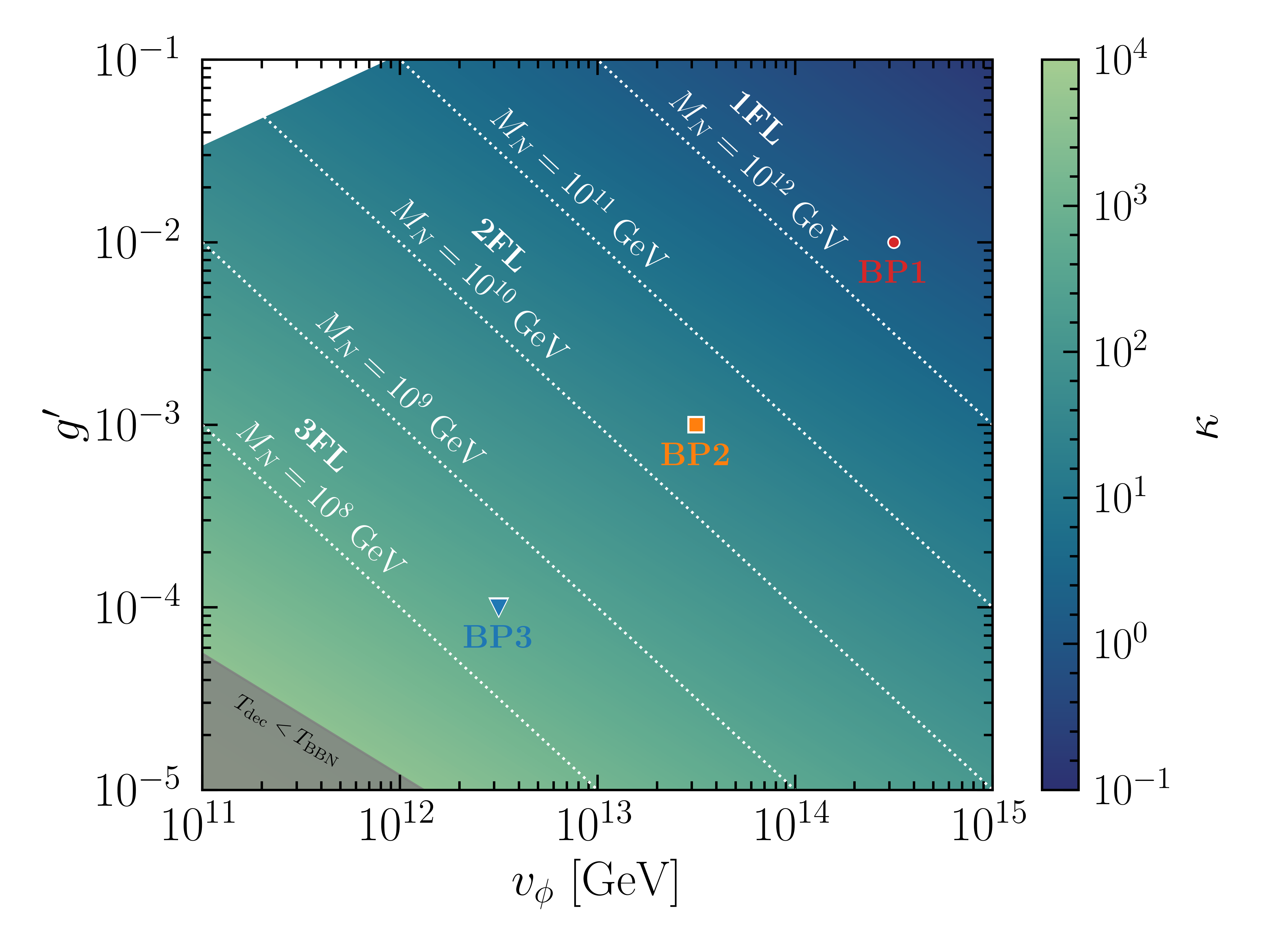
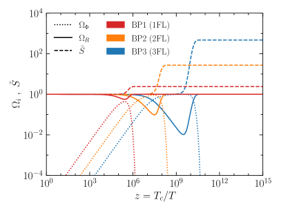
Figure 3: Left: The entropy produced by the $\Phi$ decays on the $g^{\prime}-v_{\Phi}$ plane. In this plot, the right-handed neutrino mass scale reads as $M_{N}\sim g^{\prime}v_{\Phi}$. The white region in the top-left corner is excluded because $\Gamma_{\Phi}^{f\bar{f}V}>\Gamma_{\Phi}^{hh}$. The grey-shaded region in the bottom-left corner is excluded by BBN considerations (otherwise the BBN would occur in matter domination). Right: the evolution of the normalized energy density $\Omega_{i}=\rho_{i}/\rho_{\rm tot}$ for radiation (solid lines) and $\Phi$ scalar (dotted lines), and the total entropy (dashed lines) as a function of the inverse temperature. The colour codes for the benchmarks are the same as in the left panel plot. Because the ratio of the entropy after and before the decay is important, the initial value of $\tilde{S}$ has been chosen as $\tilde{S}(z=1)=1$. The parameter $\kappa$ in Eq. (II.16) is therefore $\kappa=\tilde{S}_{\rm after}=\tilde{S}\left(z\rightarrow\infty\right)$.

Benchmark cases	$~{}~{}v_{\Phi}~{}[{\rm GeV}]~{}~{}$	$g^{\prime}$	$~{}~{}T_{\rm dom}~{}[{\rm GeV}]~{}~{}$	$~{}~{}T_{\rm dec}~{}[{\rm GeV}]~{}~{}$
BP1 (1FL)	$10^{14.5}$	$~{}~{}10^{-2}~{}~{}$	$\sim 2.8\times 10^{8}$	$\sim 2.1\times 10^{8}$
BP2 (2FL)	$10^{13.5}$	$~{}~{}10^{-3}~{}~{}$	$\sim 8.9\times 10^{5}$	$\sim 3.7\times 10^{4}$
BP3 (3FL)	$10^{12.5}$	$~{}~{}10^{-4}~{}~{}$	$\sim 2.8\times 10^{3}$	$\sim 6.6$

Table 1: The three benchmark points considered in the present paper. They corresponds to different leptogenesis mass scale $M_{N}=10^{12.5}~{}{\rm GeV}$, $M_{N}=10^{10.5}~{}{\rm GeV}$ and $M_{N}=10^{8.5}~{}{\rm GeV}$, and therefore to different leptogenesis regimes, i.e., one-flavoured (or vanilla), two-flavoured, and three-flavoured leptogenesis, respectively. In each flavour regime, leptogenesis occurs in the standard radiation domination because $T_{\rm lepto}\sim M_{N}>T_{\rm dom}$, where $T_{\rm dom}$ is the temperature at which the scalar field starts to dominate.

In Fig. 3 we show the produced entropy on the allowed model parameter space (left plot) and the evolution of the normalised energy densities $\Omega_{i}=\rho_{i}/\rho_{\rm tot}$ and the entropy (right plot) for the three sets of benchmark parameters (see Tab. 1): BP1 ($g^{\prime}=10^{-2},~{}v_{\Phi}=10^{14.5}$ GeV), BP2 ($g^{\prime}=10^{-3},~{}v_{\Phi}=10^{13.5}$ GeV), BP3 ($g^{\prime}=10^{-4},~{}v_{\Phi}=10^{12.5}$ GeV). The benchmark points are chosen such that each falls into a specific regime of leptogenesis: BP (1, 2, 3) are in one-flavoured (or vanilla), two-flavoured, and three-flavoured regime, respectively. In the left plot, the white region in the top-left corner is excluded because $g^{\prime}$ is bounded from above due to the requirement of $\Gamma_{\Phi}^{hh}>\Gamma_{\Phi}^{f\bar{f}V}$ according to Eq. (II.11), while BBN excludes the grey area according to Eq. (II.18). We find that despite large initial energy, the entropy production is less for large $v_{\Phi}$ because of the shorter lifetime of $\Phi$. We have also checked that the analytical expression for the entropy production factor $\kappa$ in Eq. (II.16) matches the numerical result (Fig. 3, right) with good accuracy.

Let us conclude this section with the following remarks: First, as it is obvious from Fig. 3 (right), the scalar field energy density $\rho_{\Phi}(T_{c})$ is always sub-dominant than the radiation energy density at $T=T_{c}$. Therefore, the universe never encounters an exponential expansion, i.e., a second period of inflation. Second, this article does not present any detailed computation related to the baryon asymmetry (we present an order of magnitude estimation in the next section). We, however, note that the baryon asymmetry produced by the RH neutrinos will also be diluted due to entropy production given in Eq. (II.16). Therefore, unlike the conventional choice of a strong hierarchy in the RH neutrino masses, a more suitable option would be to make RH neutrinos quasi-degenerate. This not only evades the issue of entropy dilution by enhancing baryon asymmetry via the resonant-leptogenesis mechanism [37], but also justifies our choice of a single RH neutrino mass scale $M_{i}\equiv M_{N}$ throughout.

III Imprints of Flavour regimes of leptogenesis on BGWs

In what follows, we briefly discuss the GW production during inflation and their propagation through multiple cosmological epochs until today. The perturbed FLRW line element that describes GWs is given by

$${\rm d}s^{2}=a(\tau)\left[-{\rm d}\tau^{2}+(\delta_{ij}+h_{ij}){\rm d}x^{\rm i}dx^{j})\right]\,,$$ (III.1)

where $\tau$ is the conformal time, and $a(\tau)$ is the scale factor. The transverse and traceless ($\partial_{i}h^{ij}=0$, $\delta^{ij}h_{ij}=0$) part of $h_{ij}$ represents the GWs. Because the GWs are weak, $|h_{ij}|\ll 1$, the following linearized evolution equation

$$\partial_{\mu}(\sqrt{-g}\partial^{\mu}h_{ij})=16\pi a^{2}(\tau)\mathcal{\pi}_{ij}$$ (III.2)

is sufficient to study the propagation of the GWs. The quantity $\pi_{ij}$ represents an anisotropy stress tensor that couples to $h_{ij}$ as an external source, which within a realistic cosmic setting only affects the GWs at large scales (than those of PTAs), e.g., due to the free streaming of light neutrinos [71, 72]. The Fourier space decomposition of $h_{ij}$ reads

$$h_{ij}(\tau,\vec{x})=\sum_{\lambda}\int\frac{{\rm d}^{3}\vec{k}}{(2\pi)^{3/2}}e^{i\vec{k}.\vec{x}}\epsilon_{ij}^{\lambda}(\vec{k})h_{\vec{k}}^{\lambda}(\tau)\,,$$ (III.3)

where the index $\lambda=``+/-"$ represents two polarisation states. The polarisation tensor $\epsilon_{ij}^{\lambda}(\vec{k})$ besides being transverse and traceless, complies with the following conditions: $\epsilon^{(\lambda)ij}(\vec{k})\epsilon_{ij}^{(\lambda^{\prime})}(\vec{k})=2\delta_{\lambda\lambda^{\prime}}$ and $\epsilon^{(\lambda)}_{ij}(-\vec{k})=\epsilon^{(\lambda)}_{ij}(\vec{k})$. Assuming isotropy and similar evolution of each polarisation state, we replace $h_{\vec{k}}^{\lambda}(\tau)$ with $h_{k}(\tau)$, where $k=|\vec{k}|=2\pi f$ with $f$ being the present frequency at $a_{0}=1$. Neglecting subdominant contribution from $\pi_{ij}$, the GW propagation equation in the Fourier space reads

$$\ddot{h}_{k}+2\frac{\dot{a}}{a}\dot{h}_{k}+k^{2}h_{k}=0\,,$$ (III.4)

where the dot represents a conformal time derivative. Using Eq. (III.3) and Eq. (III.4), the energy density of the GWs can be computed as [73]

$$\rho_{\rm GW}=\frac{1}{32\pi G}\int\frac{{\rm d}k}{k}\left(\frac{k}{a}\right)^{2}T_{T}^{2}(\tau,k)P_{T}(k)\,,$$ (III.5)

where $T_{T}^{2}(\tau,k)=|h_{k}(\tau)|^{2}/|h_{k}(\tau_{i})|^{2}$ is a transfer function with $\tau_{i}$ as the initial conformal time. The quantity $P_{T}(k)=k^{3}|h_{k}(\tau_{i})|^{2}/\pi^{2}$ characterizes the primordial power spectrum and connects to the inflation models with specific forms. Here we opt for a power-law parametrization of $P_{T}$:

$$P_{T}(k)=rA_{s}(k_{*})\left(\frac{k}{k_{*}}\right)^{n_{T}}\,,$$ (III.6)

where $r\lesssim 0.06$ [74] is the tensor-to-scalar-ratio, and $A_{s}\simeq 2\times 10^{-9}$ is the scalar perturbation amplitude at the pivot scale $k_{*}=0.01~{}{\rm Mpc^{-1}}$. In the present analysis, we take $r=0.06$ and consider the tensor spectral index $n_{T}$ constant plus blue-tilted ($n_{T}>0$). However, a scale dependence might arise owing to the higher order corrections [75] depending on the inflation model, which we do not discuss here. The normalized GW energy density pertinent to detection purposes is expressed as

$$\Omega_{\rm GW}(k)=\frac{k}{\rho_{c}}\frac{{\rm d}\rho_{\rm GW}}{{\rm d}k}\,,$$ (III.7)

where $\rho_{c}=3\mathcal{H}_{0}^{2}/8\pi G$ with $\mathcal{H}_{0}\simeq 2.2\times 10^{-4}~{}\rm Mpc^{-1}$ being the Hubble constant. From Eq. (III.5), the quantity $\Omega_{\rm GW}(k)$ is derived as

$$\Omega_{\rm GW}(k)=\frac{1}{12\mathcal{H}_{0}^{2}}\left(\frac{k}{a_{0}}\right)^{2}T_{T}^{2}(\tau_{0},k)P_{T}(k)\,,~{}~{}\tau_{0}=1.4\times 10^{4}{\rm~{}Mpc}\,.$$ (III.8)

The transfer function can be computed analytically, matching numerical results with a fair accuracy [77, 78, 79, 80, 81, 82]. When an intermediate matter domination (recall that a RH neutrino mass-dependent intermediate matter domination is the central theme of this article) is at play, $T_{T}^{2}(\tau_{0},k)$ can be calculated as [81, 82]

$$T_{T}^{2}(\tau_{0},k)=F(k)\,T_{1}^{2}(\zeta_{\rm eq})\,T_{2}^{2}(\zeta_{\Phi})\,T_{3}^{2}(\zeta_{\Phi R})\,T_{2}^{2}(\zeta_{R})\,,$$ (III.9)

where the individual transfer functions read as

$$T_{1}^{2}(\zeta) = 1+1.57\,\zeta+3.42\,\zeta^{2}\,,$$ (III.10)

$$T_{2}^{2}(\zeta) = \left(1-0.22\,\zeta^{1.5}+0.65\,\zeta^{2}\right)^{-1}\,,$$ (III.11)

$$T_{3}^{2}(\zeta) = 1+0.59\,\zeta+0.65\,\zeta^{2}\,,$$ (III.12)

with $\zeta_{i}=k/k_{i}$. The modes $k_{i}$ given by

$$k_{\rm eq} = 7.1\times 10^{-2}\Omega_{m}h^{2}{\rm Mpc^{-1}}\,\,\,{\rm with}\,\,\,\Omega_{m}=0.31\,,\,\,\,h=0.7\,,$$ (III.13)

$$k_{\Phi} = 1.7\times 10^{14}\left(\frac{g_{*s}(T_{\rm dec})}{106.75}\right)^{1/6}\left(\frac{T_{\rm dec}}{10^{7}\rm GeV}\right){\rm Mpc^{-1}}\,,$$ (III.14)

$$k_{\Phi R} = 1.7\times 10^{14}\kappa^{2/3}\left(\frac{g_{*s}(T_{\rm dec})}{106.75}\right)^{1/6}\left(\frac{T_{\rm dec}}{10^{7}\rm GeV}\right){\rm Mpc^{-1}}\,,$$ (III.15)

$$k_{R} = 1.7\times 10^{14}\kappa^{-1/3}\left(\frac{g_{*s}(T_{R})}{106.75}\right)^{1/6}\left(\frac{T_{R}}{10^{7}\rm GeV}\right){\rm Mpc^{-1}}\,,$$ (III.16)

re-enter the horizon at $T_{\rm eq}$ (the standard matter-radiation equality temperature), at $T_{\rm dec}$ (the temperature at which the scalar field decays), at $T_{\rm dom}$ (the temperature at which the scalar field starts to dominate) and at $T_{R}$ (when the universe reheats after inflation), respectively. In our computation, we use the analytical expression for $\kappa$ presented in Eq. (II.16). Notice that we have to consider the reheating after inflation precedes the phase transition of $\Phi$, i.e., $T_{R}>T_{c}$. For the following numerical analysis, we restrict ourselves to the most conservative value $T_{R}\simeq T_{c}$, which does not contradict the condition for thermal leptogenesis $T_{R}>M_{N}$ because $T_{c}>M_{N}$ (see Eq. (II.6)). The quantity $F(k)$ in Eq. (III.9) is given by

$$F(k)=\Omega_{m}^{2}\left(\frac{g_{*}(T_{k,\rm in})}{g_{*0}}\right)\left(\frac{g_{*0s}}{g_{*s}(T_{k,\rm in})}\right)^{4/3}\left(\frac{3j_{1}(k\tau_{0})}{k\tau_{0}}\right)^{2}\,,$$ (III.17)

where $T_{k,\rm in}$ is the temperature corresponding to the horizon entry of the $k$th mode, $j_{1}(k\tau_{0})$ is the spherical Bessel function, $g_{*0}=3.36$, $g_{*0s}=3.91$, and an approximate form of the scale-dependent $g_{*}$ is given by [83, 84, 82]

$$g_{*(s)}(T_{k,\rm in})=g_{*0(s)}\left(\frac{A+{\tanh k_{1}}}{A+1}\right)\left(\frac{B+{\tanh k_{2}}}{B+1}\right)\,,$$ (III.18)

where

$$A=\frac{-1-10.75/g_{*0(s)}}{-1+10.75/g_{*0(s)}}\,,~{}~{}B=\frac{-1-g_{\rm max}/10.75}{-1+g_{\rm max}/10.75}\,,$$ (III.19)

and

$$k_{1}=-2.5~{}\log_{10}\left(\frac{k/2\pi}{2.5\times 10^{-12}~{}{\rm Hz}}\right)\,,~{}~{}k_{2}=-2.0~{}{\log}_{10}\left(\frac{k/2\pi}{6.0\times 10^{-9}~{}{\rm Hz}}\right)\,,$$ (III.20)

with $g_{\rm max}$ being $\simeq 106.75$. With the above set of equations, we now evaluate the normalized GW energy density $\Omega_{\rm GW}(k)$ in Eq. (III.8) for the benchmark parameters considered in the previous section and reported in Tab. 1. Before we present the numerical results, Let us point out that the quantity $\Omega_{\rm GW}(k)h^{2}$ is constrained by two robust bounds on the Stochastic Gravitational Wave Background (SGWB) placed by the effective number of relativistic species during Big Bang Nucleosynthesis (BBN) [85] and by the LIGO measurements [86]. In particular, the BBN constraint reads

$$\int_{f_{\rm low}}^{f_{\rm high}}{\rm d}f~{}f^{-1}\Omega_{\rm GW}(f)h^{2}\lesssim 5.6\times 10^{-6}\Delta N_{\rm eff}\,,$$ (III.21)

with $\Delta N_{\rm eff}\lesssim 0.2$. The lower limit of the integration is the frequency that represents the mode entering the horizon at the BBN epoch, which we take as $f_{\rm low}\simeq 10^{-10}$ Hz. The upper limit should be the highest frequency of the GWs determined by the Hubble scale at the end of inflation $f_{\rm high}=a_{\rm end}H_{\rm end}/2\pi$. For numerical purposes, a choice $f_{\rm high}\simeq 10^{5}$ Hz would suffice as the spectrum falls and the integration saturates at higher frequencies. For the LIGO constraint, we rely on a crude estimation by considering a reference frequency $f_{\rm LIGO}=35~{}{\rm Hz}$ and discarding the GWs having an amplitude more than $6.8\times 10^{-9}$ at $f_{\rm LIGO}$ [87].

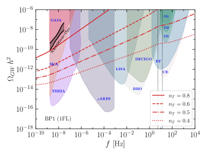
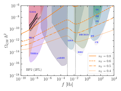
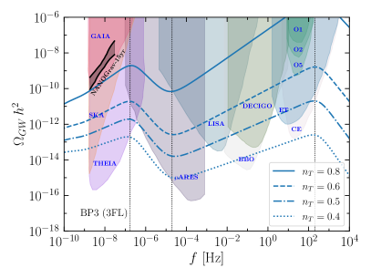
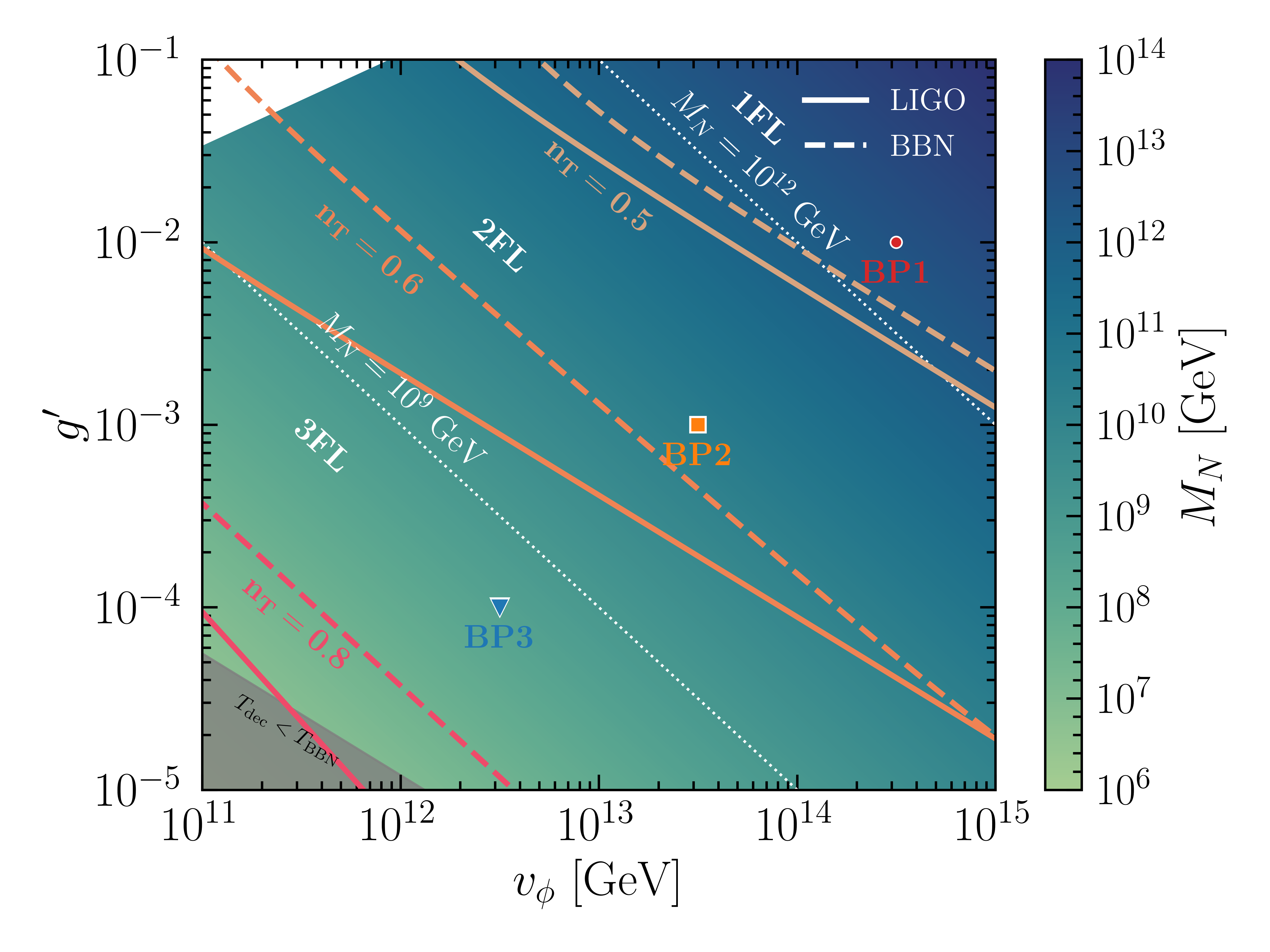
Figure 4: GW spectra for four different values of the tensor spectral index $n_{T}$. Top-left: BP1 (one-flavour regime), top-right: BP2 (two-flavour regime), bottom-left: BP3 (three-flavour regime). The shaded regions are sensitivity curves of various GW experiments such as SKA [88], GAIA and THEIA [89], $\mu$ARES [90], LISA [91], BBO [92], DECIGO [93], ET [94], CE [95], and LIGO-O5 [96]. The black bands in the nHz region represent the NANOGrav 15yrs data posteriors [6]. The dotted vertical lines (from left to right) correspond to $f^{\rm peak}_{\rm low}$, $f_{\rm dip}$ and $f^{\rm peak}_{\rm high}$, respectively. Bottom right: LIGO (solid) and BBN (dashed) constraints on the $g^{\prime}$ and $v_{\Phi}$ plane for different values of $n_{T}$. Anything above these lines is excluded. Note that LIGO constraint is much more stronger than the BBN one, implying that a viable tomography of flavoured leptogenesis with BGWs can be done only for $n_{T}\lesssim 0.8$.

In Fig. 4, we present the spectral features of the BGWs induced by the $\Phi$ matter domination set by the RH neutrino mass scale. In the top and bottom-left panels, we show the normalized GW energy density as a function of the frequency for different tensor spectral index $n_{T}$ for the three leptogenesis benchmark points representing three different flavour regimes. Notice that irrespective of the spectral index $n_{T}$, the overall spectrum gets more suppressed for large entropy production. In addition, the red tilt in the middle becomes more prominent because longer duration of $\Phi$ domination delays the horizon entry of scales $k^{-1}\in\left[k_{\Phi}^{-1},k_{\Phi R}^{-1}\right]$, and the corresponding amplitude within these $k$ values get reduced. Therefore, as the RH neutrino mass scale decreases (e.g. going from BP1 to BP3), one gets a more distinct double-peaked spectrum. As such, a three-flavour leptogenesis scenario (BP3: bottom-left panel) would predict a more distinct double peak spectrum than a two-flavour (BP2: top-right panel) or one-flavour (BP1: top-left panel) scenario. In addition to that, starting from a one-flavour/vanilla regime, as a leptogenesis scenario goes deep into the flavour regime, the low-frequency peak shifts towards lower frequencies. As evident from Fig. 4, the low-frequency peak for BP2 (two-flavour scenario) falls within the LISA (mHz) sensitivity [91], whereas, for BP3 (three-flavour scenario), it falls in the $\mu$Hz region, i.e., within the sensitivity range of THEIA [89] and $\mu$ARES [90]. Using Eq.s (III.14), (III.16) and (II.16), below we present analytical expressions for the three frequencies

$$f_{\rm low}^{\rm peak}=5.47\times 10^{-6}\left(\frac{M_{N}}{10^{9}~{}\rm GeV}\right)^{3/2}\left(\frac{g^{\prime}}{10^{-3}}\right)^{3/4}\left(\frac{g_{*s}(T_{\Phi})}{106.75}\right)^{1/6}~{}{\rm Hz}\,.$$ (III.22)

$$f_{\rm dip}\simeq 2.9\times 10^{-4}\left(\frac{M_{N}}{10^{9}~{}\rm GeV}\right)^{7/6}\left(\frac{g^{\prime}}{10^{-3}}\right)^{7/12}\left(\frac{g_{*s}(T_{\Phi})}{106.75}\right)^{1/6}~{}{\rm Hz}\,,$$ (III.23)

$$f^{\rm peak}_{\rm high}\simeq 3\times 10^{2}\left(\frac{M_{N}}{10^{9}~{}\rm GeV}\right)^{7/6}\left(\frac{g^{\prime}}{10^{-3}}\right)^{-5/12}\left(\frac{g_{*s}(T_{R})}{106.75}\right)^{1/6}~{}{\rm Hz}\,,$$ (III.24)

which determine the characteristic GW spectrum corresponding to the different regimes (because they depend on $M_{N}$) of leptogenesis. In Fig. 5, we concisely illustrate the above discussion.

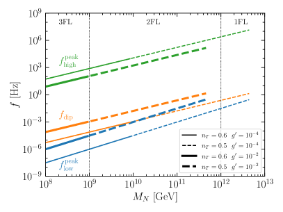
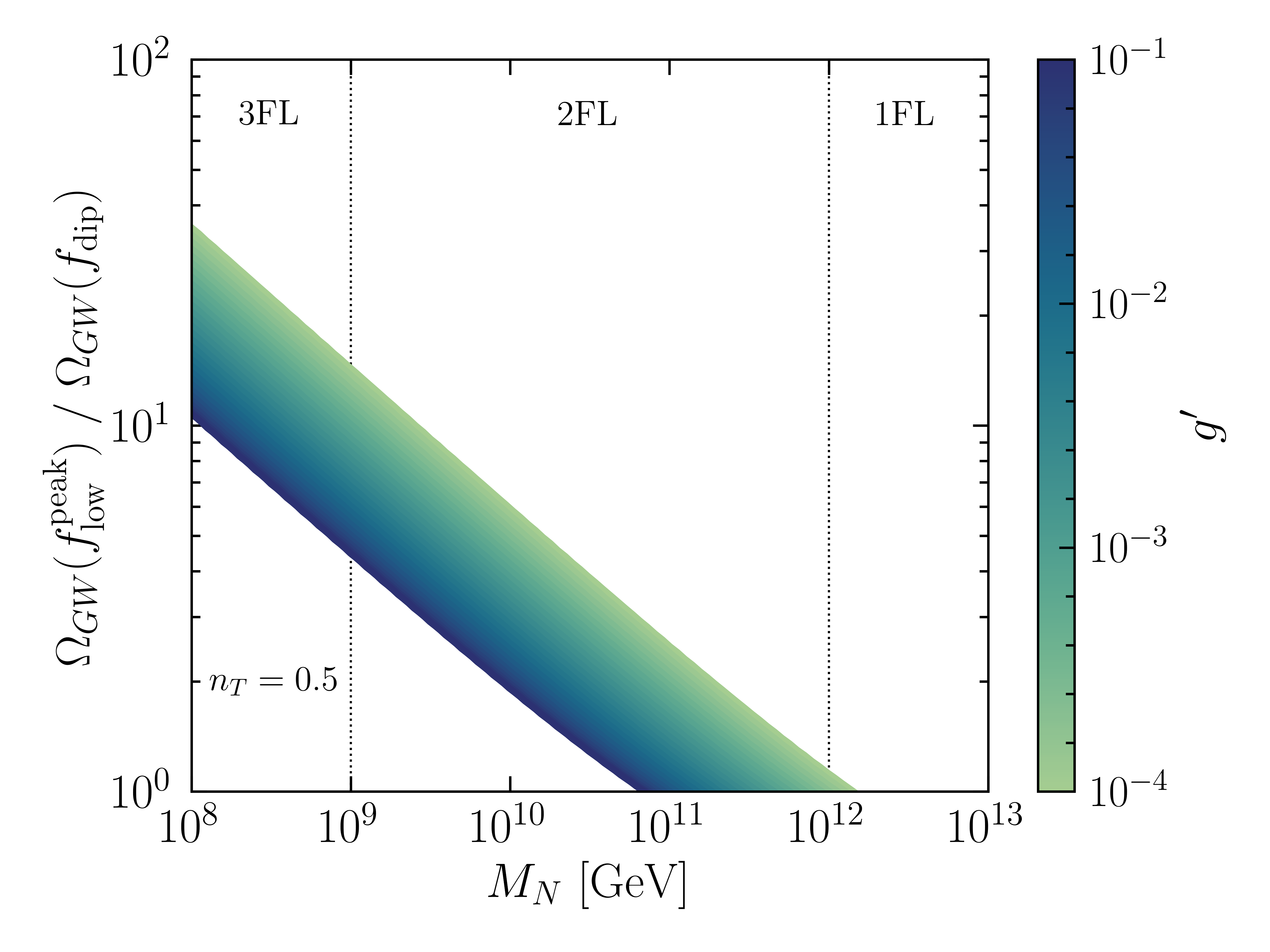
Figure 5: Left: Three frequencies, $f_{\rm low}^{\rm peak}$, $f_{\rm dip}$, and $f^{\rm peak}_{\rm high}$, describing the characteristic GW spectrum for different regimes of leptogenesis. The LIGO constraint on SGWB [87] creates the discontinuity in the curves at the end. Right: This plot quantitatively describes that as the leptogenesis process enters deep into the flavour regimes, the double peak feature in the GW spectrum becomes more prominent; the ratio $\Omega_{\rm GW}(f_{\rm low}^{\rm peak})/\Omega_{\rm GW}(f_{\rm dip})$ increases.

We now discuss the implications of the BBN and LIGO constraints on $\Omega_{\rm GW}$. In the bottom-right plot in Fig. 4, we show such constraints with solid (LIGO) and dashed (BBN) lines for different values of $n_{T}$. The parameter space above these lines is excluded. Notice that these constraints on $\Omega_{GW}$ correspond to bounds on the model parameter space and, remarkably, on the RH neutrino mass scale. In particular, the LIGO constraint is much stronger than BBN, ruling out the entire parameter space under consideration for $n_{T}=0.8$. The allowed parameter space opens for smaller values of $n_{T}$. We find that the three-flavour (two-flavour) regime is allowed in case of $n_{T}=0.6$ ($n_{T}=0.5$), while for $n_{T}<0.5$ most of the model parameter space evades all the GW bounds. An important aspect of the obtained GW spectrum is that the overall amplitude increases with $n_{T}$, and the spectrum spans a wide range of frequencies. Therefore, one way to predict robustly testable GW signal is to fix a UV model that would predict a particular value of $n_{T}$ ($\lesssim 0.8$ for the flavoured leptogenesis model as discussed here), which is not our approach. Another way, which we discuss here, is to take an IR approach by being agnostic about the source of the BGWs and treating $n_{T}$ as a free parameter. In this case, if we are able to fit a GW signal within a certain frequency band for a particular or a range of $n_{T}$ values, we can robustly predict the GW spectrum with distinct spectral features testable at a different frequency band. As such, as shown in Fig. 4 (bottom-left), a three-flavour leptogenesis scenario can predict a testable signal in the LIGO-O5 band for $n_{T}\gtrsim 0.6$. Therefore, if the future LIGO run finds a stochastic GW signal aligned with our anticipation, a three-flavour leptogenesis scenario would predict a signal with the similar spectral slope in the LISA range, distinct spectral behaviour in the $\mu$Hz range plus a testable blue tilted signal at the nHz frequencies. We can in fact compare this signal in the nHz band with the recent PTA data. For this, Let us first opt for the PTA parameterization for the $\Omega_{\rm GW}(f)$, which reads:

$$\Omega_{\rm GW}(f)=\Omega_{\rm yr}\left(\frac{f}{f_{\rm yr}}\right)^{(5-\gamma)}\,,$$ (III.25)

where $\Omega_{\rm yr}=2\pi^{2}A^{2}f_{\rm yr}^{2}/(3H_{0}^{2})$, $f_{\rm yr}=1~{}{\rm yr^{-1}}\simeq 32~{}{\rm nHz}$ with $A$ and $\gamma$ being the amplitude and spectral index. In the PTA frequency band, the $\Omega_{\rm GW}(f)$ in Eq. (III.8) is basically $\Omega_{\rm GW}(f)\propto f^{n_{T}}$, because in this range, $T_{1}(\xi)$ dominates, and we can approximate $j_{1}(k\tau_{0})\simeq 1/k\tau_{0}$. As a result, the power spectrum $P_{T}(k)$ in Eq. (III.6) determines the overall spectral shape. We can therefore compare Eq. (III.25) and Eq. (III.8) to extract $A$ and $\gamma$. In Fig. 6, we show the $A$ and $\gamma$ corresponding to BP3 with $n_{T}=0.6$ (Fig. 4, three-flavour leptogenesis scenario) with the blue triangle. The blue contours represent the $68\%$ and $95\%$ CL posteriors of NANOGrav 15-yrs data (here we chose NANOGrav posteriors for illustration), while the orange contours represent the $68\%$ and $95\%$ CL posteriors predicted for GW-driven supermassive black hole binary populations with circular orbits [10]. The black dashed lines represent the best-fit spectral index value $\gamma=3.2$ of NANOGrav 15-yrs data and the analytically predicted spectral index value $\gamma=13/3$ for GW-driven SMBHB models [98]. First, note that the spectral index is $\gamma=5-n_{T}=4.4$ (the blue triangle) for our chosen GW spectrum. Although this value could be well inside $99\%$ CL of NANOGrav data (we do not show the posterior here), the GW spectrum predicts $A\sim A^{\rm SMBHB}$, which is in tension with the NANOGrav data as shown in Fig. 6. Now, as discussed, with our BP3, a fit to an observation of SGWB by LIGO-O5 would imply a robustly testable signal in the nHz range but with $A\sim A^{\rm SMBHB}$. Therefore, if the recent PTA finding persists, then future non-observation of nHz GWs with $A\sim A^{\rm SMBHB}$ would imply that BP3 (or, more generally, a part of our model parameter space) would be ruled out. In fact, we think that the GW spectrum around BP3 ($n_{T}=0.6$) is the most promising spectrum that the discussed flavoured leptogenesis scenario offers. This is because, in this ballpark, GWs, apart from having amplitudes $A\sim A^{\rm SMBHB}$ at nHz and $A\sim A^{\rm LIGO-O5}$ at Hz, exhibit prominent and testable spectral features in the $\mu$Hz and mHz bands. A higher value of $n_{T}$ saturates LIGO and BBN bounds as shown in Fig. 4 (this is the reason that our scenario never produces a signal with $A\sim A^{\rm PTAs}$), on the other hand, for smaller $n_{T}$, the overall amplitude decreases, and the spectrum loses its testability.

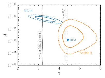
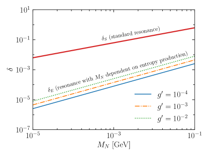
Figure 6: Left: Comparison of GW amplitude and spectral indices: The blue contours represent the $68\%$ and $95\%$ CL posteriors of NANOGrav 15-yrs data. The orange contours represent the $68\%$ and $95\%$ CL posteriors predicted for GW-driven supermassive black hole binary populations with circular orbits [10]. The vertical dashed lines represent the best-fit values $\gamma=3.2$ of NANOGrav 15-yrs data and analytically predicted value $\gamma=13/3$ for GW-driven SMBHB models [98]. The blue triangle denotes $A$ and $\gamma$ corresponding to the BP3 with $n_{T}=0.6$ in our discussion, representing a three-flavour regime of leptogenesis. Right: RH neutrino mass splitting as a function of the RH neutrino mass scale $M_{N}$. The red curve represents the mass splitting for the standard resonance leptogenesis scenario without entropy production. The other three gauge coupling-dependent curves represent the same but with an RH neutrino mass-dependent entropy production scenario. All these curves are consistent with the observed value of the baryon to photon ratio $\eta_{B}\simeq 6.3\times 10^{-10}$. For details, see text.

We would like to conclude with the following remarks. First, a generic feature of $\Omega_{\rm GW}\propto f^{n_{T}\gg 0}$ is that the spectrum does not span a wide range of frequency due to the BBN bound on effective neutrino species. Therefore, cosmologically viable inflationary BGWs require a low reheating temperature after inflation. This has been discussed in detail in the literature and recently in the context of PTA results [15]. However, when an intermediate matter-dominated epoch is at play, the spectrum may span a wide range of frequencies without violating any cosmological bounds because of the entropy injection. It allows a high $T_{R}$, which is notably, also a natural requirement for high-scale thermal leptogenesis, as we discuss here. Let us also stress that our results depend on the parameterization of the primordial power spectrum in Eq. (III.6). A different parameterization [82, 99, 100, 101] would yield different results.

Second, since the last couple of years, there has been an effort to test leptogenesis with primordial GWs, see, e.g., Refs. [69, 102, 103, 104, 105, 106, 107, 108, 109, 110, 111]. This article, nonetheless, for the first time, attempts to probe flavour regimes of leptogenesis with GWs. We would also like to point out a technical aspect of the leptogenesis computation, which differs from the standard scenario. Because of the larger entropy production and stronger baryon asymmetry dilution for smaller RH neutrino masses, our scenario requires more quasi-degenerate RH neutrinos than the standard case as the RH neutrino mass scale decreases. This can be understood in the following way. The produced baryon-to-photon ratio in the resonance regime can be written as [37]

$$\eta_{B}=10^{-2}\varepsilon_{i}\zeta_{i}\kappa^{-1}\,\,\,{\rm with}\,\,\,\varepsilon_{i}\simeq\frac{3M_{i}\overline{m}}{8\pi v_{h}^{2}\delta}\,,$$ (III.26)

where $\varepsilon_{i}$ is the CP asymmetry parameter, $\zeta_{i}\simeq 10^{-1}$ is the efficiency of lepton asymmetry production, $\overline{m}\simeq 0.1$ eV is the light neutrino mass scale, $\delta=(M_{j}-M_{i})/{M_{i}}$, $v_{h}=174$ GeV is the SM Higgs vacuum expectation value, and $\kappa$ is the injected entropy by $\Phi$ decay as defined in Eq. (II.16). We can obtain an expression for $\delta$ in two cases. The standard case without entropy production corresponds to $\kappa=1$. Given the observed value $\eta_{B}\simeq 6.3\times 10^{-10}$ [112], using Eq. (III.26), we obtain

$$\delta_{S} \simeq 6.25\times 10^{-1}\left(\frac{M_{N}}{10^{9}\rm GeV}\right)\,,$$ (III.27)

$$\delta_{E} \simeq 4.5\times 10^{-3}\left(\frac{g^{\prime}}{10^{-3}}\right)^{1/4}\left(\frac{M_{N}}{10^{9}\rm GeV}\right)^{3/2}\,,$$ (III.28)

where the subscript $S(E)$ represents the mass splitting in the standard (with entropy production) case. Here, we assume $M_{i}\equiv M_{N}$ and simplify $\kappa$ in Eq. (II.16) in terms of our model parameters as

$$\kappa\simeq 140\left(\frac{g^{\prime}}{10^{-3}}\right)^{-1/4}\left(\frac{M_{N}}{10^{9}\rm GeV}\right)^{-1/2}.$$ (III.29)

In Fig. 6 (right) we show $\delta_{E,\>S}$ as a function of $M_{N}$. Note that while $\delta_{E}$ is always smaller than $\delta_{S}$, it becomes even smaller as $M_{N}$ decreases. In this context, we can also make an interesting observation that in this GW tomography method, more is the quasi-degeneracy in the RH neutrino masses more distinct is the spectral feature in the GWs. This is because, as discussed already, $\Omega_{\rm GW}(f_{\rm low}^{\rm peak})/\Omega_{\rm GW}(f_{\rm dip})$ increases with the decrease of $M_{N}$.

Finally, because we consider a $U(1)$ gauge symmetry breaking, our scenario must produce cosmic strings [113], which is another source of GWs [114]. We nonetheless note that we work with unconventional parameter space, which in the numerical simulations of the cosmic strings evolution are taken as $g^{\prime}\sim~{}\mathcal{O}(1)$ and $\lambda\sim~{}\mathcal{O}(1)$ [115, 116]. If we, in any case, assume that for smaller values of these coupling, the GW computation from cosmic strings holds, we might obtain interesting spectral features in the cosmic strings radiated GWs because of the discussed RH neutrino mass-dependent intermediate matter domination. This, however, is beyond the scope of this paper, and we shall present a semi-analytical description of the prospects of GWs from cosmic strings in our scenario in a future publication.

IV Summary

In the present paper, for the first time, we show that flavour regimes of thermal leptogenesis can be markedly tested with gravitational waves’ spectral features. Flavour effects bridge high-scale leptogenesis and low-energy neutrino physics and are important in leptogenesis computation. We opt for a tomographic method, where gravitational waves originating from an independent source, confront the leptogenesis model during their propagation in the early universe and carry imprints of leptogenesis parameters on the final gravitational waves spectrum. There are three distinct regimes of flavoured leptogenesis characterized by the right-handed neutrino mass scale: $M_{N}\gtrsim 10^{12}~{}{\rm GeV}$ (one-flavour/vanilla), $10^{9}~{}{\rm GeV}\lesssim M_{N}\lesssim 10^{12}~{}{\rm GeV}$ (two-flavour), and $M_{N}\lesssim 10^{9}~{}{\rm GeV}$ (three-flavour). Testing flavour regimes with gravitational waves is thus equivalent to studying detectable spectral features in the gravitational waves dependent on the mass scale $M_{N}$. This is possible in the simplest and well-motivated realizations of seesaw scenarios that facilitate a scalar field to give mass to the right-handed neutrinos. Apart from generating right-handed neutrino masses, the scalar field can be long-lived to provide a matter-dominated epoch with a lifetime depending on $M_{N}$. When gravitational waves pass through such a matter-dominated phase, the start, the end, and the duration of the matter-domination get imprinted on the final gravitational waves spectrum. Thus in our case, the spectral features in the GWs become dependent on $M_{N}$, hence on different regimes of leptogenesis. While any gravitational waves that originate prior to the scalar field domination can offer a viable tomography, here we consider inflationary blue gravitational waves, which are now being widely discussed after the recent finding of blue stochastic gravitational waves by the Pulsar Timing Arrays, with an infra-red tail characterized by a simple power-law $\Omega_{\rm GW}\sim f^{n_{T}}$. We show that owing to the scalar field domination, the final gravitational waves exhibit a double peak spectrum, with the characteristic frequencies depending on $M_{N}$. As the leptogenesis process enters deep into the flavour regimes, the spectral features in the gravitational waves become more prominent, and the characteristic frequencies shift to lower values (see Figs. 4 and 5). As such, for a two-flavour (three-flavour) regime, the low-frequency peak shows up in the mHz ($\mu$Hz) bands. While the BBN constraint on the effective number of neutrino species and LIGO bound on stochastic gravitational waves background restrict the spectral index value $n_{T}\lesssim 0.8$ (see Fig. 4, bottom-right), a three-flavour leptogenesis scenario offers the most promising signal for $n_{T}\sim 0.6-0.7$. Indeed, it shows an amplitude testable in the next LIGO run at $f\sim$ Hz, characteristic spectral features in the mHz and $\mu$Hz bands (see Fig. 4, bottom-left), plus a refutable gravitational wave strain at $f\sim$ nHz, comparable to the one expected from supermassive black holes (see Fig. 6, left, the blue triangle).

References

- Guth [1981] A. H. Guth, The Inflationary Universe: A Possible Solution to the Horizon and Flatness Problems, Phys. Rev. D 23, 347 (1981).
- Linde [1982] A. D. Linde, A New Inflationary Universe Scenario: A Possible Solution of the Horizon, Flatness, Homogeneity, Isotropy and Primordial Monopole Problems, Phys. Lett. B 108, 389 (1982).
- Datta and Samanta [2022] S. Datta and R. Samanta, Gravitational waves-tomography of Low-Scale-Leptogenesis, JHEP 11, 159, arXiv:2208.09949 [hep-ph] .
- Datta and Samanta [2023] S. Datta and R. Samanta, Fingerprints of GeV scale right-handed neutrinos on inflationary gravitational waves and PTA data, Phys. Rev. D 108, L091706 (2023), arXiv:2307.00646 [hep-ph] .
- Fukugita and Yanagida [1986] M. Fukugita and T. Yanagida, Baryogenesis Without Grand Unification, Phys. Lett. B 174, 45 (1986).
- Agazie et al. [2023a] G. Agazie et al. (NANOGrav), The NANOGrav 15 yr Data Set: Evidence for a Gravitational-wave Background, Astrophys. J. Lett. 951, L8 (2023a), arXiv:2306.16213 [astro-ph.HE] .
- Antoniadis et al. [2023] J. Antoniadis et al. (EPTA, InPTA:), The second data release from the European Pulsar Timing Array - III. Search for gravitational wave signals, Astron. Astrophys. 678, A50 (2023), arXiv:2306.16214 [astro-ph.HE] .
- Reardon et al. [2023] D. J. Reardon et al., Search for an Isotropic Gravitational-wave Background with the Parkes Pulsar Timing Array, Astrophys. J. Lett. 951, L6 (2023), arXiv:2306.16215 [astro-ph.HE] .
- Xu et al. [2023] H. Xu et al., Searching for the Nano-Hertz Stochastic Gravitational Wave Background with the Chinese Pulsar Timing Array Data Release I, Res. Astron. Astrophys. 23, 075024 (2023), arXiv:2306.16216 [astro-ph.HE] .
- Afzal et al. [2023] A. Afzal et al. (NANOGrav), The NANOGrav 15 yr Data Set: Search for Signals from New Physics, Astrophys. J. Lett. 951, L11 (2023), arXiv:2306.16219 [astro-ph.HE] .
- Vagnozzi [2021] S. Vagnozzi, Implications of the NANOGrav results for inflation, Mon. Not. Roy. Astron. Soc. 502, L11 (2021), arXiv:2009.13432 [astro-ph.CO] .
- Bhattacharya et al. [2021] S. Bhattacharya, S. Mohanty, and P. Parashari, Implications of the NANOGrav result on primordial gravitational waves in nonstandard cosmologies, Phys. Rev. D 103, 063532 (2021), arXiv:2010.05071 [astro-ph.CO] .
- Kuroyanagi et al. [2021] S. Kuroyanagi, T. Takahashi, and S. Yokoyama, Blue-tilted inflationary tensor spectrum and reheating in the light of NANOGrav results, JCAP 01, 071, arXiv:2011.03323 [astro-ph.CO] .
- Benetti et al. [2022] M. Benetti, L. L. Graef, and S. Vagnozzi, Primordial gravitational waves from NANOGrav: A broken power-law approach, Phys. Rev. D 105, 043520 (2022), arXiv:2111.04758 [astro-ph.CO] .
- Vagnozzi [2023] S. Vagnozzi, Inflationary interpretation of the stochastic gravitational wave background signal detected by pulsar timing array experiments, JHEAp 39, 81 (2023), arXiv:2306.16912 [astro-ph.CO] .
- Borah et al. [2024] D. Borah, S. Jyoti Das, and R. Samanta, Imprint of inflationary gravitational waves and WIMP dark matter in pulsar timing array data, JCAP 03, 031, arXiv:2307.00537 [hep-ph] .
- DeRocco and Dror [2024] W. DeRocco and J. A. Dror, Using Pulsar Parameter Drifts to Detect Subnanohertz Gravitational Waves, Phys. Rev. Lett. 132, 101403 (2024), arXiv:2212.09751 [astro-ph.HE] .
- DeRocco and Dror [2023] W. DeRocco and J. A. Dror, Searching for stochastic gravitational waves below a nanohertz, Phys. Rev. D 108, 103011 (2023), arXiv:2304.13042 [astro-ph.HE] .
- Blas and Jenkins [2022a] D. Blas and A. C. Jenkins, Bridging the Hz Gap in the Gravitational-Wave Landscape with Binary Resonances, Phys. Rev. Lett. 128, 101103 (2022a), arXiv:2107.04601 [astro-ph.CO] .
- Blas and Jenkins [2022b] D. Blas and A. C. Jenkins, Detecting stochastic gravitational waves with binary resonance, Phys. Rev. D 105, 064021 (2022b), arXiv:2107.04063 [gr-qc] .
- Bari et al. [2022] P. Bari, A. Ricciardone, N. Bartolo, D. Bertacca, and S. Matarrese, Signatures of Primordial Gravitational Waves on the Large-Scale Structure of the Universe, Phys. Rev. Lett. 129, 091301 (2022), arXiv:2111.06884 [astro-ph.CO] .
- Gruzinov [2004] A. Gruzinov, Elastic inflation, Phys. Rev. D 70, 063518 (2004), arXiv:astro-ph/0404548 .
- Kobayashi et al. [2010] T. Kobayashi, M. Yamaguchi, and J. Yokoyama, G-inflation: Inflation driven by the Galileon field, Phys. Rev. Lett. 105, 231302 (2010), arXiv:1008.0603 [hep-th] .
- Endlich et al. [2013] S. Endlich, A. Nicolis, and J. Wang, Solid Inflation, JCAP 10, 011, arXiv:1210.0569 [hep-th] .
- Cannone et al. [2015] D. Cannone, G. Tasinato, and D. Wands, Generalised tensor fluctuations and inflation, JCAP 01, 029, arXiv:1409.6568 [astro-ph.CO] .
- Ricciardone and Tasinato [2017] A. Ricciardone and G. Tasinato, Primordial gravitational waves in supersolid inflation, Phys. Rev. D 96, 023508 (2017), arXiv:1611.04516 [astro-ph.CO] .
- Cai et al. [2015] Y.-F. Cai, J.-O. Gong, S. Pi, E. N. Saridakis, and S.-Y. Wu, On the possibility of blue tensor spectrum within single field inflation, Nucl. Phys. B 900, 517 (2015), arXiv:1412.7241 [hep-th] .
- Fujita et al. [2019] T. Fujita, S. Kuroyanagi, S. Mizuno, and S. Mukohyama, Blue-tilted Primordial Gravitational Waves from Massive Gravity, Phys. Lett. B 789, 215 (2019), arXiv:1808.02381 [gr-qc] .
- Mishima and Kobayashi [2020] Y. Mishima and T. Kobayashi, Revisiting slow-roll dynamics and the tensor tilt in general single-field inflation, Phys. Rev. D 101, 043536 (2020), arXiv:1911.02143 [gr-qc] .
- Pan et al. [2024] S. Pan, Y. Cai, and Y.-S. Piao, Climbing over the potential barrier during inflation via null energy condition violation, (2024), arXiv:2404.12655 [astro-ph.CO] .
- Datta [2023] S. Datta, Explaining PTA Data with Inflationary GWs in a PBH-Dominated Universe, (2023), arXiv:2309.14238 [hep-ph] .
- Kuzmin et al. [1985] V. A. Kuzmin, V. A. Rubakov, and M. E. Shaposhnikov, On the Anomalous Electroweak Baryon Number Nonconservation in the Early Universe, Phys. Lett. B 155, 36 (1985).
- Alvarez-Gaume and Witten [1984] L. Alvarez-Gaume and E. Witten, Gravitational Anomalies, Nucl. Phys. B 234, 269 (1984).
- Alexander et al. [2006] S. H.-S. Alexander, M. E. Peskin, and M. M. Sheikh-Jabbari, Leptogenesis from gravity waves in models of inflation, Phys. Rev. Lett. 96, 081301 (2006), arXiv:hep-th/0403069 .
- Cohen and Kaplan [1987] A. G. Cohen and D. B. Kaplan, Thermodynamic Generation of the Baryon Asymmetry, Phys. Lett. B 199, 251 (1987).
- Riotto and Trodden [1999] A. Riotto and M. Trodden, Recent progress in baryogenesis, Ann. Rev. Nucl. Part. Sci. 49, 35 (1999), arXiv:hep-ph/9901362 .
- Pilaftsis and Underwood [2004] A. Pilaftsis and T. E. J. Underwood, Resonant leptogenesis, Nucl. Phys. B 692, 303 (2004), arXiv:hep-ph/0309342 .
- Buchmuller et al. [2005] W. Buchmuller, P. Di Bari, and M. Plumacher, Leptogenesis for pedestrians, Annals Phys. 315, 305 (2005), arXiv:hep-ph/0401240 .
- Davidson et al. [2008] S. Davidson, E. Nardi, and Y. Nir, Leptogenesis, Phys. Rept. 466, 105 (2008), arXiv:0802.2962 [hep-ph] .
- Bodeker and Buchmuller [2021] D. Bodeker and W. Buchmuller, Baryogenesis from the weak scale to the grand unification scale, Rev. Mod. Phys. 93, 035004 (2021), arXiv:2009.07294 [hep-ph] .
- Di Bari [2022] P. Di Bari, On the origin of matter in the Universe, Prog. Part. Nucl. Phys. 122, 103913 (2022), arXiv:2107.13750 [hep-ph] .
- Davidson and Ibarra [2002] S. Davidson and A. Ibarra, A Lower bound on the right-handed neutrino mass from leptogenesis, Phys. Lett. B 535, 25 (2002), arXiv:hep-ph/0202239 .
- Akhmedov et al. [1998] E. K. Akhmedov, V. A. Rubakov, and A. Y. Smirnov, Baryogenesis via neutrino oscillations, Phys. Rev. Lett. 81, 1359 (1998), arXiv:hep-ph/9803255 .
- Hambye and Teresi [2016] T. Hambye and D. Teresi, Higgs doublet decay as the origin of the baryon asymmetry, Phys. Rev. Lett. 117, 091801 (2016), arXiv:1606.00017 [hep-ph] .
- Bhupal Dev et al. [2014] P. S. Bhupal Dev, P. Millington, A. Pilaftsis, and D. Teresi, Flavour Covariant Transport Equations: an Application to Resonant Leptogenesis, Nucl. Phys. B 886, 569 (2014), arXiv:1404.1003 [hep-ph] .
- Abada et al. [2006] A. Abada, S. Davidson, A. Ibarra, F. X. Josse-Michaux, M. Losada, and A. Riotto, Flavour Matters in Leptogenesis, JHEP 09, 010, arXiv:hep-ph/0605281 .
- Nardi et al. [2006] E. Nardi, Y. Nir, E. Roulet, and J. Racker, The Importance of flavor in leptogenesis, JHEP 01, 164, arXiv:hep-ph/0601084 .
- Blanchet and Di Bari [2007] S. Blanchet and P. Di Bari, Flavor effects on leptogenesis predictions, JCAP 03, 018, arXiv:hep-ph/0607330 .
- Pascoli et al. [2007] S. Pascoli, S. T. Petcov, and A. Riotto, Leptogenesis and Low Energy CP Violation in Neutrino Physics, Nucl. Phys. B 774, 1 (2007), arXiv:hep-ph/0611338 .
- Altarelli and Feruglio [2010] G. Altarelli and F. Feruglio, Discrete Flavor Symmetries and Models of Neutrino Mixing, Rev. Mod. Phys. 82, 2701 (2010), arXiv:1002.0211 [hep-ph] .
- King [2017] S. F. King, Unified Models of Neutrinos, Flavour and CP Violation, Prog. Part. Nucl. Phys. 94, 217 (2017), arXiv:1701.04413 [hep-ph] .
- Davidson [1979] A. Davidson, as the fourth color within an model, Phys. Rev. D 20, 776 (1979).
- Marshak and Mohapatra [1980] R. E. Marshak and R. N. Mohapatra, Quark - Lepton Symmetry and B-L as the U(1) Generator of the Electroweak Symmetry Group, Phys. Lett. B 91, 222 (1980).
- Mohapatra and Marshak [1980] R. N. Mohapatra and R. E. Marshak, Local B-L Symmetry of Electroweak Interactions, Majorana Neutrinos and Neutron Oscillations, Phys. Rev. Lett. 44, 1316 (1980), [Erratum: Phys.Rev.Lett. 44, 1643 (1980)].
- Buchmüller et al. [2013] W. Buchmüller, V. Domcke, K. Kamada, and K. Schmitz, The Gravitational Wave Spectrum from Cosmological Breaking, JCAP 10, 003, arXiv:1305.3392 [hep-ph] .
- Buchmuller et al. [2020] W. Buchmuller, V. Domcke, H. Murayama, and K. Schmitz, Probing the scale of grand unification with gravitational waves, Phys. Lett. B 809, 135764 (2020), arXiv:1912.03695 [hep-ph] .
- Minkowski [1977] P. Minkowski, at a Rate of One Out of Muon Decays?, Phys. Lett. B 67, 421 (1977).
- Gell-Mann et al. [1979] M. Gell-Mann, P. Ramond, and R. Slansky, Complex Spinors and Unified Theories, Conf. Proc. C 790927, 315 (1979), arXiv:1306.4669 [hep-th] .
- Yanagida [1980] T. Yanagida, Horizontal Symmetry and Masses of Neutrinos, Prog. Theor. Phys. 64, 1103 (1980).
- Mohapatra [1986] R. N. Mohapatra, Mechanism for Understanding Small Neutrino Mass in Superstring Theories, Phys. Rev. Lett. 56, 561 (1986).
- Linde [1979] A. D. Linde, Phase Transitions in Gauge Theories and Cosmology, Rept. Prog. Phys. 42, 389 (1979).
- Kibble [1980] T. W. B. Kibble, Some Implications of a Cosmological Phase Transition, Phys. Rept. 67, 183 (1980).
- Quiros [1999] M. Quiros, Finite temperature field theory and phase transitions, in ICTP Summer School in High-Energy Physics and Cosmology (1999) pp. 187–259, arXiv:hep-ph/9901312 .
- Caprini et al. [2016] C. Caprini et al., Science with the space-based interferometer eLISA. II: Gravitational waves from cosmological phase transitions, JCAP 04, 001, arXiv:1512.06239 [astro-ph.CO] .
- Hindmarsh et al. [2021] M. B. Hindmarsh, M. Lüben, J. Lumma, and M. Pauly, Phase transitions in the early universe, SciPost Phys. Lect. Notes 24, 1 (2021), arXiv:2008.09136 [astro-ph.CO] .
- Megevand and Ramirez [2017] A. Megevand and S. Ramirez, Bubble nucleation and growth in very strong cosmological phase transitions, Nucl. Phys. B 919, 74 (2017), arXiv:1611.05853 [astro-ph.CO] .
- Gross et al. [2016] C. Gross, O. Lebedev, and M. Zatta, Higgs–inflaton coupling from reheating and the metastable Universe, Phys. Lett. B 753, 178 (2016), arXiv:1506.05106 [hep-ph] .
- Enqvist et al. [2016] K. Enqvist, M. Karciauskas, O. Lebedev, S. Rusak, and M. Zatta, Postinflationary vacuum instability and Higgs-inflaton couplings, JCAP 11, 025, arXiv:1608.08848 [hep-ph] .
- Blasi et al. [2020] S. Blasi, V. Brdar, and K. Schmitz, Fingerprint of low-scale leptogenesis in the primordial gravitational-wave spectrum, Phys. Rev. Res. 2, 043321 (2020), arXiv:2004.02889 [hep-ph] .
- Croon et al. [2019] D. Croon, N. Fernandez, D. McKeen, and G. White, Stability, reheating and leptogenesis, JHEP 06, 098, arXiv:1903.08658 [hep-ph] .
- Weinberg [2004] S. Weinberg, Damping of tensor modes in cosmology, Phys. Rev. D 69, 023503 (2004), arXiv:astro-ph/0306304 .
- Zhao et al. [2009] W. Zhao, Y. Zhang, and T. Xia, New method to constrain the relativistic free-streaming gas in the Universe, Phys. Lett. B 677, 235 (2009), arXiv:0905.3223 [astro-ph.CO] .
- Page et al. [2007] L. Page et al. (WMAP), Three year Wilkinson Microwave Anisotropy Probe (WMAP) observations: polarization analysis, Astrophys. J. Suppl. 170, 335 (2007), arXiv:astro-ph/0603450 .
- Ade et al. [2018] P. A. R. Ade et al. (BICEP2, Keck Array), BICEP2 / Keck Array x: Constraints on Primordial Gravitational Waves using Planck, WMAP, and New BICEP2/Keck Observations through the 2015 Season, Phys. Rev. Lett. 121, 221301 (2018), arXiv:1810.05216 [astro-ph.CO] .
- Kuroyanagi and Takahashi [2011] S. Kuroyanagi and T. Takahashi, Higher Order Corrections to the Primordial Gravitational Wave Spectrum and its Impact on Parameter Estimates for Inflation, JCAP 10, 006, arXiv:1106.3437 [astro-ph.CO] .
- Liddle and Lyth [1993] A. R. Liddle and D. H. Lyth, The Cold dark matter density perturbation, Phys. Rept. 231, 1 (1993), arXiv:astro-ph/9303019 .
- Seto and Yokoyama [2003] N. Seto and J. Yokoyama, Probing the equation of state of the early universe with a space laser interferometer, J. Phys. Soc. Jap. 72, 3082 (2003), arXiv:gr-qc/0305096 .
- Boyle and Steinhardt [2008] L. A. Boyle and P. J. Steinhardt, Probing the early universe with inflationary gravitational waves, Phys. Rev. D 77, 063504 (2008), arXiv:astro-ph/0512014 .
- Nakayama et al. [2008] K. Nakayama, S. Saito, Y. Suwa, and J. Yokoyama, Probing reheating temperature of the universe with gravitational wave background, JCAP 06, 020, arXiv:0804.1827 [astro-ph] .
- Kuroyanagi et al. [2009] S. Kuroyanagi, T. Chiba, and N. Sugiyama, Precision calculations of the gravitational wave background spectrum from inflation, Phys. Rev. D 79, 103501 (2009), arXiv:0804.3249 [astro-ph] .
- Nakayama and Yokoyama [2010] K. Nakayama and J. Yokoyama, Gravitational Wave Background and Non-Gaussianity as a Probe of the Curvaton Scenario, JCAP 01, 010, arXiv:0910.0715 [astro-ph.CO] .
- Kuroyanagi et al. [2015] S. Kuroyanagi, T. Takahashi, and S. Yokoyama, Blue-tilted Tensor Spectrum and Thermal History of the Universe, JCAP 02, 003, arXiv:1407.4785 [astro-ph.CO] .
- Watanabe and Komatsu [2006] Y. Watanabe and E. Komatsu, Improved Calculation of the Primordial Gravitational Wave Spectrum in the Standard Model, Phys. Rev. D 73, 123515 (2006), arXiv:astro-ph/0604176 .
- Saikawa and Shirai [2018] K. Saikawa and S. Shirai, Primordial gravitational waves, precisely: The role of thermodynamics in the Standard Model, JCAP 05, 035, arXiv:1803.01038 [hep-ph] .
- Peimbert et al. [2016] A. Peimbert, M. Peimbert, and V. Luridiana, The primordial helium abundance and the number of neutrino families, Rev. Mex. Astron. Astrofis. 52, 419 (2016), arXiv:1608.02062 [astro-ph.CO] .
- Abbott et al. [2017a] B. P. Abbott et al. (LIGO Scientific, Virgo), Upper Limits on the Stochastic Gravitational-Wave Background from Advanced LIGO’s First Observing Run, Phys. Rev. Lett. 118, 121101 (2017a), [Erratum: Phys.Rev.Lett. 119, 029901 (2017)], arXiv:1612.02029 [gr-qc] .
- Abbott et al. [2021a] R. Abbott et al. (KAGRA, Virgo, LIGO Scientific), Upper limits on the isotropic gravitational-wave background from Advanced LIGO and Advanced Virgo’s third observing run, Phys. Rev. D 104, 022004 (2021a), arXiv:2101.12130 [gr-qc] .
- Weltman et al. [2020] A. Weltman et al., Fundamental physics with the Square Kilometre Array, Publ. Astron. Soc. Austral. 37, e002 (2020), arXiv:1810.02680 [astro-ph.CO] .
- Garcia-Bellido et al. [2021] J. Garcia-Bellido, H. Murayama, and G. White, Exploring the early Universe with Gaia and Theia, JCAP 12 (12), 023, arXiv:2104.04778 [hep-ph] .
- Sesana et al. [2021] A. Sesana et al., Unveiling the gravitational universe at -Hz frequencies, Exper. Astron. 51, 1333 (2021), arXiv:1908.11391 [astro-ph.IM] .
- Amaro-Seoane et al. [2017] P. Amaro-Seoane et al. (LISA), Laser Interferometer Space Antenna, (2017), arXiv:1702.00786 [astro-ph.IM] .
- Yagi and Seto [2011] K. Yagi and N. Seto, Detector configuration of DECIGO/BBO and identification of cosmological neutron-star binaries, Phys. Rev. D 83, 044011 (2011), [Erratum: Phys.Rev.D 95, 109901 (2017)], arXiv:1101.3940 [astro-ph.CO] .
- Kawamura et al. [2006] S. Kawamura et al., The Japanese space gravitational wave antenna DECIGO, Class. Quant. Grav. 23, S125 (2006).
- Sathyaprakash et al. [2012] B. Sathyaprakash et al., Scientific Objectives of Einstein Telescope, Class. Quant. Grav. 29, 124013 (2012), [Erratum: Class.Quant.Grav. 30, 079501 (2013)], arXiv:1206.0331 [gr-qc] .
- Abbott et al. [2017b] B. P. Abbott et al. (LIGO Scientific), Exploring the Sensitivity of Next Generation Gravitational Wave Detectors, Class. Quant. Grav. 34, 044001 (2017b), arXiv:1607.08697 [astro-ph.IM] .
- Abbott et al. [2021b] R. Abbott et al. (KAGRA, Virgo, LIGO Scientific), Upper limits on the isotropic gravitational-wave background from Advanced LIGO and Advanced Virgo’s third observing run, Phys. Rev. D 104, 022004 (2021b), arXiv:2101.12130 [gr-qc] .
- Agazie et al. [2023b] G. Agazie et al. (International Pulsar Timing Array), Comparing recent PTA results on the nanohertz stochastic gravitational wave background, (2023b), arXiv:2309.00693 [astro-ph.HE] .
- Phinney [2001] E. S. Phinney, A Practical theorem on gravitational wave backgrounds, (2001), arXiv:astro-ph/0108028 .
- Jiang et al. [2023] J.-Q. Jiang, Y. Cai, G. Ye, and Y.-S. Piao, Broken blue-tilted inflationary gravitational waves: a joint analysis of NANOGrav 15-year and BICEP/Keck 2018 data, (2023), arXiv:2307.15547 [astro-ph.CO] .
- Cai and Piao [2021] Y. Cai and Y.-S. Piao, Intermittent null energy condition violations during inflation and primordial gravitational waves, Phys. Rev. D 103, 083521 (2021), arXiv:2012.11304 [gr-qc] .
- Giarè et al. [2023] W. Giarè, M. Forconi, E. Di Valentino, and A. Melchiorri, Towards a reliable calculation of relic radiation from primordial gravitational waves, Mon. Not. Roy. Astron. Soc. 520, 2 (2023), arXiv:2210.14159 [astro-ph.CO] .
- Dror et al. [2020] J. A. Dror, T. Hiramatsu, K. Kohri, H. Murayama, and G. White, Testing the Seesaw Mechanism and Leptogenesis with Gravitational Waves, Phys. Rev. Lett. 124, 041804 (2020), arXiv:1908.03227 [hep-ph] .
- Samanta and Datta [2021] R. Samanta and S. Datta, Gravitational wave complementarity and impact of NANOGrav data on gravitational leptogenesis, JHEP 05, 211, arXiv:2009.13452 [hep-ph] .
- Datta et al. [2021] S. Datta, A. Ghosal, and R. Samanta, Baryogenesis from ultralight primordial black holes and strong gravitational waves from cosmic strings, JCAP 08, 021, arXiv:2012.14981 [hep-ph] .
- Barman et al. [2022] B. Barman, D. Borah, A. Dasgupta, and A. Ghoshal, Probing high scale Dirac leptogenesis via gravitational waves from domain walls, Phys. Rev. D 106, 015007 (2022), arXiv:2205.03422 [hep-ph] .
- Dasgupta et al. [2022] A. Dasgupta, P. S. B. Dev, A. Ghoshal, and A. Mazumdar, Gravitational wave pathway to testable leptogenesis, Phys. Rev. D 106, 075027 (2022), arXiv:2206.07032 [hep-ph] .
- Borah et al. [2023] D. Borah, S. Jyoti Das, R. Samanta, and F. R. Urban, PBH-infused seesaw origin of matter and unique gravitational waves, JHEP 03, 127, arXiv:2211.15726 [hep-ph] .
- Perez-Gonzalez and Turner [2021] Y. F. Perez-Gonzalez and J. Turner, Assessing the tension between a black hole dominated early universe and leptogenesis, Phys. Rev. D 104, 103021 (2021), arXiv:2010.03565 [hep-ph] .
- Ghoshal et al. [2023] A. Ghoshal, R. Samanta, and G. White, Bremsstrahlung high-frequency gravitational wave signatures of high-scale nonthermal leptogenesis, Phys. Rev. D 108, 035019 (2023), arXiv:2211.10433 [hep-ph] .
- Huang and Xie [2022] P. Huang and K.-P. Xie, Leptogenesis triggered by a first-order phase transition, JHEP 09, 052, arXiv:2206.04691 [hep-ph] .
- Borah et al. [2022] D. Borah, A. Dasgupta, and I. Saha, Leptogenesis and dark matter through relativistic bubble walls with observable gravitational waves, JHEP 11, 136, arXiv:2207.14226 [hep-ph] .
- Ade et al. [2016] P. A. R. Ade et al. (Planck), Planck 2015 results. XIII. Cosmological parameters, Astron. Astrophys. 594, A13 (2016), arXiv:1502.01589 [astro-ph.CO] .
- Kibble [1976] T. W. B. Kibble, Topology of Cosmic Domains and Strings, J. Phys. A 9, 1387 (1976).
- Vilenkin [1981] A. Vilenkin, Gravitational radiation from cosmic strings, Phys. Lett. B 107, 47 (1981).
- Blanco-Pillado et al. [2011] J. J. Blanco-Pillado, K. D. Olum, and B. Shlaer, Large parallel cosmic string simulations: New results on loop production, Phys. Rev. D 83, 083514 (2011), arXiv:1101.5173 [astro-ph.CO] .
- Matsunami et al. [2019] D. Matsunami, L. Pogosian, A. Saurabh, and T. Vachaspati, Decay of Cosmic String Loops Due to Particle Radiation, Phys. Rev. Lett. 122, 201301 (2019), arXiv:1903.05102 [hep-ph] .