Abstract

In this study, we investigate agent-based approach for system model identification with an emphasis on power distribution system applications. Departing from conventional practices of relying on historical data for offline model identification, we adopt an online update approach utilizing real-time data by employing the latest data points for gradient computation. This methodology offers advantages including a large reduction in the communication network’s bandwidth requirements by minimizing the data exchanged at each iteration and enabling the model to adapt in real-time to disturbances. Furthermore, we extend our model identification process from linear frameworks to more complex non-linear convex models. This extension is validated through numerical studies demonstrating improved control performance for a synthetic IEEE test case.

keywords: Data-driven control, distributed optimization, model identification, online optimization, power grids.

A Distributed Model Identification Algorithm for Multi-Agent Systems Vivek Khatana, Chin-Yao Chang, Wenbo Wang V, Khatana is with Department of Electrical and Computer Engineering, University of Minnesota, Minneapolis, USA (Email: {khata010}@umn.edu).C.-Y. Chang and W. Wang are with the National Renewable Energy Laboratory, Golden, CO 80401, USA (Email: {chinyao.chang, wenbo.wang}@nrel.gov). This work was authored in part by NREL, operated by Alliance for Sustainable Energy, LLC, for the U.S. Department of Energy (DOE) under Contract No. DE-AC36-08GO28308. Funding provided by DOE Office of Electricity, Advanced Grid Modeling Program, through agreement NO. 33652. The views expressed in the article do not necessarily represent the views of the DOE or the U.S. Government. The U.S. Government retains and the publisher, by accepting the article for publication, acknowledges that the U.S. Government retains a nonexclusive, paid-up, irrevocable, worldwide license to publish or reproduce the published form of this work, or allow others to do so, for U.S. Government purposes.

I Introduction

System model identification is pivotal across numerous applications, where comprehending underlying processes is crucial for effective control and decision-making. Due to the complexity and dynamic nature of these systems, precise model identification is foundational to predictive analytics and system optimization. In this paper, we consider the following model formulation:

$\displaystyle y(t)=g(u(t),\theta)$ (1)

where $u(t)\in\mathbb{R}^{\mathbf{d_{u}}}$ and $y(t)\in\mathbb{R}^{\mathbf{d_{y}}}$ denote the input and output data at time $t$, and $\theta\in\mathbb{R}^{\mathbf{d}_{\theta}}$ contains the parameters to be identified. We define the dataset $\mathcal{M}:=\{(u(t),y(t))\}_{t=1}^{T}$ compiled from inputs and outputs across times $t=1,\cdots,T$, and aim to identify the optimal parameter $\theta^{*}$ that minimizes:

$\displaystyle\textstyle\mathbf{r}(\theta)=\frac{1}{2}\sum_{t=1}^{T}\left\lVert y(t)-g(u(t),\theta)\right\rVert^{2}.$ (2)

In the context of power systems, especially at the distribution levels, model identification can be crucial for determining system topology, the LinDistFlow model, or the admittance matrix [1, 2, 3, 4], which are essential for controlling power networks. Traditional approaches whether through conventional methods or machine learning techniques, typically rely on centralized data collection and processing. However, we contend that the decentralized nature of modern power systems, particularly with the increasing integration of distributed energy resources, calls for a multi-agent-based distributed approach [5, 6]. This strategy not only facilitates the autonomous operation of individual system components but also enhances the overall resilience of the network. Distributed algorithms promote localized decision-making, substantially reducing communication overhead and the risk of single points of failure inherent in centralized systems. Building on this foundation, our previous work [7] advanced distributed identification methods that protect local data privacy, although it was restricted to linear systems and demanded high bandwidth communication.

Building on the merits of the distributed and localized approach from our prior research, this paper introduces several advancements: (i) We have developed a distributed method for the identification of nonlinear systems using local input-output data; (ii) Our algorithm requires agents to use only current measurements for updates, thereby eliminating the need for storing historical data and substantially reducing communication bandwidth requirements. Moreover, it facilitates the sharing of non-linear estimates between agents during updates, enhancing the protection of individual agent parameters. (iii) Numerical studies demonstrate that identifying more accurate nonlinear models results in superior control performance compared to traditional linear models, underscoring the practical value of our advancements.

Notations and definitions: In this paper, we denote matrices in boldface. Let $\operatorname{diag}{(x)}$ represent the matrix whose diagonal elements are the elements of the vector $x\in\mathbb{R}^{n}$. For matrices $\mathbf{A}^{1},\mathbf{A}^{2},\cdots,\mathbf{A}^{N}\in\mathbb{R}^{m\times n}$, we denote $\operatorname{blkdiag}{(\{\mathbf{A}^{i}\}_{i=1}^{N})}$ as the block diagonal matrix of the matrices $\mathbf{A}^{i}$. The vertical and horizontal concatenation of matrices $\mathbf{A}^{i}$ are denoted as $[\mathbf{A}^{1};\mathbf{A}^{2};\cdots;\mathbf{A}^{n}]\in\mathbb{R}^{Nm\times n}$ and $[\mathbf{A}^{1},\mathbf{A}^{2},\cdots,\mathbf{A}^{n}]\in\mathbb{R}^{m\times Nn}$. For a matrix $\mathbf{A}\in\mathbb{R}^{m\times n}$, $\operatorname*{vec}(\mathbf{A})\in\mathbb{R}^{mn}$ is a column vector created by concatenating the column vectors of $\mathbf{A}$ from left to right. For a matrix $\mathbf{A}\in\mathbb{R}^{m\times n}$, $\operatorname{null}\{\mathbf{A}\}$ denotes the null space of matrix $\mathbf{A}$. The scalar element of the $i^{th}$ row and $j^{th}$ column of $\mathbf{A}$ is denoted as $\mathbf{A}_{ij}$ and the $j^{th}$ row and column of the matrix $\mathbf{A}$ are denoted as $\mathbf{A}_{j,:}$ and $\mathbf{A}_{:,j}$, respectively. The identity matrix and vector with all entries equal to $1$ of dimension $n$ are denoted as $\mathbf{I}_{n}$ and $1_{n}$, respectively.

A graph $\mathcal{G}$ is denoted by a pair $(\mathcal{V},\mathcal{E})$ where $\mathcal{V}$ is a set of vertices (or nodes) and $\mathcal{E}$ is a set of edges, which are ordered subsets of two distinct elements of $\mathcal{V}$. If an edge from $j\in\mathcal{V}$ to $i\in\mathcal{V}$ exists then it is denoted as $(i,j)\in\mathcal{E}$. The set of neighboring sub-systems of node $i\in\mathcal{V}$ is called the neighborhood of node $i$ and is denoted by $\operatorname{\mathcal{N}}_{i}=\{j\ |\ (i,j)\in\mathcal{E}\}$. In the subsequent, we use the terms agents, nodes, and sub-systems interchangeably. Given a norm $\|\cdot\|$ and a set $K\subset\mathbb{R}^{p}$, define the diameter of $K$ with respect to this norm as $Diam_{\|\cdot\|}(K):=\sup_{x,y\in K}\|x-y\|$. In the subsequent text the $O(.)$ and $o(.)$ operations denote the standard Big-O and Little-o notations respectively [8].

II Agent Based System Framework

In this section, we commence by demonstrating how (2) can be reinterpreted as a distributed optimization challenge across a network of sub-systems or agents. Subsequently, we delve into deriving analytical properties of these reformulations, which serve as the foundation for the convergence analysis of the online identification algorithm.

II-A Distributed input-output data framework

Consider that model (1) is represented by an underlying network $\mathcal{G}(\mathcal{V},\mathcal{E})$ consisting of $|\mathcal{V}|:=N$ sub-systems. Here, each sub-system has actuator and sensor measurements available within itself. Each agent $i\in\mathcal{V}:=\{1,2,\cdots,N\}$ has information on certain entries of the vectors $u(t)$ and $y(t)$ in (1) indexed by the sets $S^{u}_{i}\subset\{1,2,\dots,\mathbf{d_{u}}\}$ and $S^{y}_{i}\subset\{1,2,\dots,\mathbf{d_{y}}\}$ respectively. We assume the partitions $S^{u}_{i}$ and $S^{y}_{i}$ are such that $\mathbf{d_{u}}_{i}:=|S^{u}_{i}|,\sum_{i=1}^{N}\mathbf{d_{u}}_{i}=\mathbf{d_{u}},\mathbf{d_{y}}_{i}:=|S^{y}_{i}|,\sum_{i=1}^{N}\mathbf{d_{y}}_{i}=\mathbf{d_{y}}$. Let $\text{u}_{i}(t)\in\mathbb{R}^{\mathbf{d_{u}}_{i}}$ and $\text{y}_{i}(t)\in\mathbb{R}^{\mathbf{d_{y}}_{i}}$ denote the respective entries of the input and output that agent $i$ has information on. Without loss of generality, $u(t)=[\text{u}_{1}(t),\text{u}_{2}(t),\dots,\text{u}_{N}(t)]^{\top}\in\mathbb{R}^{\mathbf{d_{u}}},y(t)=[\text{y}_{1}(t),\text{y}_{2}(t),\dots,\text{y}_{N}(t)]^{\top}\in\mathbb{R}^{\mathbf{d_{y}}}$. We make the following assumption on model (1):

Assumption 1.

The system (1) is BIBO stable, i.e. any bounded input $u(t)$ yields a bounded output $y(t)$. In addition, $\exists\ \bar{u}<\infty$ such that $u(t)\leq\bar{u}$ for all time $t\in\{1,2,\dots,T\}$.

Assumption 2.

The function $g(u,\theta)$ is proper with respect to $\theta$ and is separable, i.e. $g(u,\theta)=\sum_{i=1}^{N}a_{i}\phi_{i}(\text{u}_{i},\theta_{i})$, for some $a_{i}>0$ with $\theta=[\theta_{1},\dots,\theta_{N}]$, and the functions $\phi_{i}$ are convex and Lipschitz continuous with constant $L_{i}$.

Under Assumption 2 and the network model, each agent $i$ via $\phi_{i}$ captures how its regional controls $\text{u}_{i}$ affect the output $y$ by knowing the parameter $\theta_{i}$. Therefore, the goal for each agent $i$ is identifying $\theta_{i}$ by distributed communication and computations on locally available data $\text{u}_{i}$ and $\text{y}_{i}$.

II-B Distributed reformulation of the system modeling

In this section, we go through a series of reformulations of (1) for convenience of distributed algorithm design. With Assumption 2, we have the following formulation of $\mathbf{r}(\theta)$:

$\displaystyle\textstyle\mathbf{r}(\theta)=\frac{1}{2}\sum_{t=1}^{T}\left\lVert y(t)-\sum_{i=1}^{N}a_{i}\phi_{i}(\text{u}_{i}(t),\theta_{i})\right\rVert^{2}.$ (3)

Define $\widehat{\mathbf{Y}}(t)=\operatorname{diag}{(y(t))}=\operatorname{diag}{([\text{y}_{1}(t);\dots;\text{y}_{N}(t)])}\in\mathbb{R}^{\mathbf{d_{y}}\times\mathbf{d_{y}}}$. Because $\sum_{i=1}^{N}(\sum_{j\in S^{y}_{i}}[\widehat{\mathbf{Y}}(t)]_{:,j})=y(t)$, we can re-write (3) as

$\displaystyle\textstyle\mathbf{r}(\theta)=\frac{1}{2}\sum_{t=1}^{T}\left\lVert\sum_{i=1}^{N}\big{(}\sum_{j\in S^{y}_{i}}[\widehat{\mathbf{Y}}(t)]_{:,j}-a_{i}\phi_{i}(\text{u}_{i}(t),\theta_{i})\big{)}\right\rVert^{2}.$

With the above set of reformulations, the system model identification problem is

$\displaystyle\operatorname{argmin}_{\theta}\frac{1}{2}\sum_{t=1}^{T}\left\lVert\sum_{i=1}^{N}\big{(}a_{i}\phi_{i}(\text{u}_{i}(t),\theta_{i})-\sum_{j\in S^{y}_{i}}[\widehat{\mathbf{Y}}(t)]_{:,j}\big{)}\right\rVert^{2}.$ (4)

The function $\mathbf{r}(\theta)$ couples the parameters and data for all the agents. We next consider a reformulation described in [9] to setup a formulation for the distributed algorithm, allowing the agents to do computation on locally available data and communicate with the neighboring agents in the network $\mathcal{G}(\mathcal{V},\mathcal{E})$ while recovering the solution of problem (4). Assuming the network $\mathcal{G}(\mathcal{V},\mathcal{E})$ is connected, we define $\mathbf{P}\in\mathbb{R}^{N\times N}$ as the Laplacian matrix associated with the graph. and consider the problem:

$\displaystyle\operatorname{argmin}_{\theta,w\in\mathbb{R}^{N\mathbf{d_{y}}}}\frac{1}{2}\sum_{t=1}^{T}\left\lVert\Phi_{a}(\text{u}(t),\theta)-\widehat{\mathbf{y}}(t)-\widehat{\mathbf{P}}w\right\rVert^{2},$ (5)

where $\Phi_{a}(\text{u}(t),\theta):=[a_{1}\phi_{1}(\text{u}_{1}(t),\theta_{1});a_{2}\phi_{2}(\text{u}_{2}(t),\theta_{2});\dots;$ $a_{N}\phi_{N}(\text{u}_{N}(t),\theta_{N})]\in\mathbb{R}^{N\mathbf{d_{y}}},\widehat{\mathbf{y}}:=\big{[}\sum_{j\in S^{y}_{1}}[\widehat{\mathbf{Y}}(t)]_{:,j};$ $\sum_{j\in S^{y}_{2}}[\widehat{\mathbf{Y}}(t)]_{:,j};\dots;\sum_{j\in S^{y}_{N}}[\widehat{\mathbf{Y}}(t)]_{:,j}\big{]}\in\mathbb{R}^{N\mathbf{d_{y}}},\widehat{\mathbf{P}}:=\mathbf{P}\otimes\mathbf{I}_{\mathbf{d_{y}}}$. Define $\mathbf{x}=[\theta;\widehat{\mathbf{P}}w]$, $F(\mathbf{x})=\sum_{t=1}^{T}f_{t}(\mathbf{x})$ with $f_{t}(\mathbf{x})=\frac{1}{2}\left\lVert\Phi_{a}(\text{u}(t),\theta)-\widehat{\mathbf{y}}(t)-\widehat{\mathbf{P}}w\right\rVert^{2}$ for convenience. Lemma 1 shows that the optimal solution of (5) is also a solution for (4).

Lemma 1.

(Optimal solutions of (4) and (5)). If $\mathbf{x}^{*}=(\theta^{*},\widehat{\mathbf{P}}w^{*})$ is an optimal solution of problem (5), then $\theta^{*}$ is also an optimal solution of problem (4).

Proof.

Using the first order optimality conditions for the convex function $F$ (sum of composition of convex and increasing functions), we have $\nabla_{\theta}F(\mathbf{x}^{*})=0,\;\nabla_{w}F(\mathbf{x}^{*})=0$. Namely, for all $t\in\{1,2,\dots,T\}$,

$\displaystyle\nabla_{\theta}\Phi_{a}(\text{u}(t),\theta^{*})^{\top}(\Phi_{a}(\text{u}(t),\theta^{*})-\widehat{\mathbf{y}}(t)-\widehat{\mathbf{P}}w^{*})$ $\displaystyle=0,$ (6)
$\displaystyle\widehat{\mathbf{P}}^{\top}(\Phi_{a}(\text{u}(t),\theta^{*})-\widehat{\mathbf{y}}(t)-\widehat{\mathbf{P}}w^{*})$ $\displaystyle=0.$ (7)

From the property of the Laplacian matrix, $\operatorname{null}\{\mathbf{P}\}=\operatorname{span}\{1_{N}\}$, and (7), there exists $z^{*}$ such that

$\displaystyle 1_{N}\otimes z^{*}:=(\Phi_{a}(\text{u}(t),\theta^{*})-\widehat{\mathbf{y}}(t)-\widehat{\mathbf{P}}w^{*})$ (8)

Multiplying both by $1_{N}^{\top}\otimes\mathbf{I}_{\mathbf{d_{y}}}$ we get,

$\displaystyle Nz^{*}$ $\displaystyle=(1_{N}^{\top}\otimes\mathbf{I}_{\mathbf{d_{y}}})1_{N}\otimes z^{*}$
$\displaystyle=(1_{N}^{\top}\otimes\mathbf{I}_{\mathbf{d_{y}}})(\Phi_{a}(\text{u}(t),\theta^{*})-\widehat{\mathbf{y}}(t)-\widehat{\mathbf{P}}w^{*})$
$\displaystyle\textstyle=\sum_{i=1}^{N}\big{(}a_{i}\phi_{i}(\text{u}_{i}(t),\theta_{i}^{*})-\sum_{j\in S^{y}_{i}}[\widehat{\mathbf{Y}}(t)]_{:,j}\big{)}$
$\displaystyle\hskip 21.68121pt-(1_{N}^{\top}\otimes\mathbf{I}_{\mathbf{d_{y}}})(\mathbf{P}\otimes\mathbf{I}_{\mathbf{d_{y}}})w^{*}$
$\displaystyle\textstyle=\sum_{i=1}^{N}\big{(}a_{i}\phi_{i}(\text{u}_{i}(t),\theta^{*}_{i})-\sum_{j\in S^{y}_{i}}[\widehat{\mathbf{Y}}(t)]_{:,j}\big{)}$
$\displaystyle\hskip 21.68121pt-(1_{N}^{\top}\otimes\mathbf{P})(\mathbf{I}_{\mathbf{d_{y}}}\otimes\mathbf{I}_{\mathbf{d_{y}}})w^{*}$
$\displaystyle\textstyle=\sum_{i=1}^{N}\big{(}a_{i}\phi_{i}(\text{u}_{i}(t),\theta^{*}_{i})-\sum_{j\in S^{y}_{i}}[\widehat{\mathbf{Y}}(t)]_{:,j}\big{)}.$

Thus,

$\displaystyle\textstyle z^{*}=\frac{1}{N}\Big{(}\sum_{i=1}^{N}\big{(}a_{i}\phi_{i}(\text{u}_{i}(t),\theta^{*}_{i})-\sum_{j\in S^{y}_{i}}[\widehat{\mathbf{Y}}(t)]_{:,j}\big{)}\Big{)}$ (9)

Substituting (8) and (9) in (6), we have

$\displaystyle a_{j}\nabla_{\theta_{j}}$ $\displaystyle\textstyle\phi_{a}(\text{u}_{j}(t),\theta^{*}_{j})^{\top}[\Big{(}\sum_{i=1}^{N}\big{(}a_{i}\phi_{i}(\text{u}_{i}(t),\theta_{i}^{\star})$
$\displaystyle\textstyle-\sum_{j\in S^{y}_{i}}[\widehat{\mathbf{Y}}(t)]_{:,j}\big{)}]\ =0,\;\forall j\in\{1,2,\dots,N\}.$ (10)

Because problem (4) is convex, by the optimality conditions, any $\theta^{{}^{\prime}}$ is a solution of (4) if and only if, for all $t\in\{1,\dots,T\}$,

$\displaystyle a_{j}\nabla_{\theta_{j}}\phi_{j}$ $\displaystyle\textstyle(\text{u}_{j}(t),\theta^{{}^{\prime}}_{j})^{\top}\Big{(}\sum_{i=1}^{N}\big{(}a_{i}\phi_{i}(\text{u}_{i}(t),\theta_{i}^{{}^{\prime}})$
$\displaystyle\textstyle-\sum_{j\in S^{y}_{i}}[\widehat{\mathbf{Y}}(t)]_{:,j}\big{)}\Big{)}=0,\ \forall j\in\{1,2,\dots,N\}.$

Thus, we conclude $\theta^{*}$ is a solution of (4). ∎

Lemma 1 serves as an essential step for distributed algorithm design because it enables us to focus on solving (5) instead of (4) with distributed component $\mathbf{P}$. Following this, we introduce Lemma 2, which establishes the boundedness of the gradient steps involved in addressing (5).

Lemma 2.

Let Assumptions 1-2 hold. There exists constants $\eta_{t}>0$ and $\Delta<\infty$ such that $\|\nabla f_{t}\|:=\left\|\left[\begin{array}[]{cc}\nabla_{\theta}f_{t}\\ \nabla_{w}f_{t}\end{array}\right]\right\|\leq\Delta$ for all $t\in\{1,\dots,T\}$ with $\mathbf{x}(t)$ updated by

$\displaystyle\mathbf{x}(t+1)=\mathbf{x}(t)-\eta_{t}\nabla f_{t}(\mathbf{x}(t)).$ (11)
Proof.

We start by presenting three supporting claims that we later utilize to prove the desired result.

Claim 1: Any $\gamma$ sub-level set $C_{\gamma}:=\{\mathbf{x}\ |\ f_{t}(\mathbf{x})\leq\gamma\}$ of $f_{t}$ is bounded.

Proof. Given $\beta>0$, let $v^{*}\in\operatorname{argmin}_{\mathbf{x}}f_{t}(\mathbf{x})$, with $\|v^{*}\|<\infty$. Define, $\Gamma_{\beta}:=\{\mathbf{x}\ |\ \|\mathbf{x}-v^{*}\|=\beta\}$ and $v_{\beta}=\inf_{\mathbf{x}\in\Gamma_{\beta}}f_{t}(\mathbf{x})$. Note that $\Gamma_{\beta}$ is non-empty and compact. Since, $f_{t}$ is continuous, from the Weierstrass’s theorem $v_{\beta}$ is attained at some point of $\Gamma_{\beta}$, we have $v_{\beta}>f_{t}(v^{*})$. For any $\mathbf{x}$ such that $\|\mathbf{x}-v^{*}\|>\beta$, let $\alpha=\frac{\beta}{\|\mathbf{x}-v^{*}\|},\tilde{\mathbf{x}}=(1-\alpha)v^{*}+\alpha\mathbf{x}$. By convexity of $f_{t}$, we have

$\displaystyle(1-\alpha)f_{t}(v^{*})+\alpha f_{t}(\mathbf{x})\geq f_{t}(\tilde{\mathbf{x}}).$

Since $\|\tilde{\mathbf{x}}-v^{*}\|=\alpha\|\mathbf{x}-v^{*}\|=\beta$, $\tilde{\mathbf{x}}\in\Gamma_{\beta}$ and

$\displaystyle f_{t}(\tilde{\mathbf{x}})\geq v_{\beta}=\inf_{\mathbf{x}\in\Gamma_{\beta}}f_{t}(\mathbf{x}).$

Combining the above two relations, we get

$\displaystyle f_{t}(\mathbf{x})$ $\displaystyle\textstyle\geq\frac{f_{t}(\tilde{\mathbf{x}})-f_{t}(v^{*})}{\alpha}+f_{t}(v^{*})\geq f_{t}(v^{*})+\frac{v_{\beta}-f_{t}(v^{*})}{\alpha}$
$\displaystyle=\textstyle f_{t}(v^{*})+\frac{v_{\beta}-f_{t}(v^{*})}{\beta}\|\mathbf{x}-v^{*}\|.$

Because $v_{\beta}>f_{t}(v^{*})$ and $f_{t}(\mathbf{x})\leq\gamma$, we derive

$\displaystyle\|\mathbf{x}-v^{*}\|\leq\textstyle\frac{\beta(\gamma-f_{t}(v^{*}))}{v_{\beta}-f_{t}(v^{*})}.$

Thus, $\|\mathbf{x}-v^{*}\|\leq\max\left\{\beta,\frac{\beta(\gamma-f_{t}(v^{*}))}{v_{\beta}-f_{t}(v^{*})}\right\}.\hskip 25.29494pt\qed$

Claim 2: There exists a sufficiently small $\eta_{t}>0$ such that for all $t\in\{1,2,\dots,T\}$, $\mathbf{x}(t+1)$ updated by (11) lies in the sub-level set $C_{f_{t}(\mathbf{x}(t))}:=\{\mathbf{x}\ |\ f_{t}(\mathbf{x})\leq f_{t}(\mathbf{x}(t))\}$.

Proof. By Taylor series expansion and $f_{t}\geq 0$,

$\displaystyle f_{t}(\mathbf{x}(t+1))$ $\displaystyle=f_{t}\big{(}\mathbf{x}(t)-\eta_{t}\nabla f_{t}(\mathbf{x}(t))\big{)}$
$\displaystyle=f_{t}(\mathbf{x}(t))-\eta_{t}\|\nabla f_{t}(\mathbf{x}(t))\|^{2}+o(\eta_{t}\nabla f_{t}(\mathbf{x}(t)))$
$\displaystyle=\textstyle f_{t}(\mathbf{x}(t))\!-\!\eta_{t}\left(\!\|\nabla f_{t}(\mathbf{x}(t))\|^{2}\!+\!\frac{o(\eta_{t}\nabla f_{t}(\mathbf{x}(t)))}{\eta_{t}}\!\right)\!\leq f_{t}(\mathbf{x}(t)),$

for sufficiently small $\eta_{t}>0$ by the definition of $o(\eta_{t})$, which completes the proof.

Claim 3: Let $\operatorname{\mathbf{z}}(t):=\Phi_{a}(\text{u}(t),\theta(t))-\widehat{\mathbf{y}}(t)-\widehat{\mathbf{P}}w(t)$. Then, $\exists\ \bar{\operatorname{\mathbf{z}}}<\infty$ such that $\|\operatorname{\mathbf{z}}(t)\|\leq\overline{\operatorname{\mathbf{z}}}$ for all $t\in\{1,2,\dots,T\}$.

Proof. Under Assumptions 1 and 2,

$\displaystyle\|\operatorname{\mathbf{z}}(t)-\operatorname{\mathbf{z}}(1)\|=\|\Phi_{a}(\text{u}(t),\theta(t))-\widehat{\mathbf{y}}(t)-\widehat{\mathbf{P}}w(t)\ -$
$\displaystyle\hskip 86.72377pt\Phi_{a}(\text{u}(1),\theta(1))+\widehat{\mathbf{y}}(1)+\widehat{\mathbf{P}}w(1)\|$
$\displaystyle\leq\|\big{(}\Phi_{a}(\text{u}(t),\theta(t))-\widehat{\mathbf{P}}w(t)\big{)}\ -\big{(}\Phi_{a}(\text{u}(1),\theta(1))-\widehat{\mathbf{P}}w(1)\big{)}\|$
$\displaystyle\hskip 14.45377pt+\|\widehat{\mathbf{y}}(t)-\widehat{\mathbf{y}}(1)\|$
$\displaystyle=L_{m}\left\|\left[\!\!\begin{array}[]{cc}\text{u}(t)\\ \mathbf{x}(t)\end{array}\!\!\right]-\left[\!\!\begin{array}[]{cc}\text{u}(1)\\ \mathbf{x}(1)\end{array}\!\!\right]\right\|+\|\widehat{\mathbf{y}}(t)-\widehat{\mathbf{y}}(1)\|.$

Therefore, $\|\operatorname{\mathbf{z}}(t)-\operatorname{\mathbf{z}}(1)\|\leq 2\overline{\text{y}}+2L_{m}(\overline{\text{u}}+D_{m})$, where the results of Claims 1 and 2 are applied with $D_{m}:=\max_{t}Diam_{\|.\|}(C_{f_{t}(\mathbf{x}(t))})$ and $L_{m}:=\max_{1\leq i\leq N}L_{i}$. Therefore, there exists a $\bar{\operatorname{\mathbf{z}}}<\infty$ that bounds $\|\operatorname{\mathbf{z}}(t)\|$ for all $t\in\{1,2,\dots,T\}.\qed$

With all the claims, we circle back to the proof of Lemma 2. At any time index $t$,

$\displaystyle\nabla f_{t}$ $\displaystyle=\left[\begin{array}[]{cc}\nabla_{\theta}f_{t}\\ \nabla_{w}f_{t}\end{array}\right]=\left[\begin{array}[]{cc}\nabla_{\theta}\Phi_{a}(\text{u}(t),\theta(t))^{\top}\operatorname{\mathbf{z}}(t)\\ -\widehat{\mathbf{P}}^{\top}\operatorname{\mathbf{z}}(t)\end{array}\right].$

Thus, $\|\nabla f_{t}\|^{2}\leq\|\nabla_{\theta}\Phi_{a}(\text{u}(t),\theta(t))^{\top}\operatorname{\mathbf{z}}(t)\|^{2}+\|\widehat{\mathbf{P}}^{\top}\operatorname{\mathbf{z}}(t)\|^{2}+2\|\nabla_{\theta}\Phi_{a}(\text{u}(t),\theta(t))^{\top}\operatorname{\mathbf{z}}(t)\|\|\widehat{\mathbf{P}}^{\top}\operatorname{\mathbf{z}}(t)\|\leq(NL_{m}+\|\widehat{\mathbf{P}}\|)^{2}\overline{\operatorname{\mathbf{z}}}^{2}$, where we used Assumption 2 and claim 3. Hence, $\|\nabla f_{t}\|\leq(NL_{m}+\|\widehat{\mathbf{P}}\|)\overline{\operatorname{\mathbf{z}}}:=\Delta$. This completes the proof. ∎

III Distributed Model identification

In this section, we develop an online algorithm designed to address the system model identification problem as formulated in (5). Subsequently, we elucidate the methodology for implementing this online algorithm within a distributed framework.

III-A Model identification via online experiments

We begin the section by assuming that the input-output data for the system for every time instant in a sequential manner are available. In such a setting, the experimental data appears as an infinite sequence $(u(1),y(1)),(u(2),y(2)),(u(3),y(3)),\dots$. At any time $t$ after $(u(t),y(t))$ is obtained, the error function $f_{t}(\mathbf{x})$ is presented. As the information is received sequentially and all information is not available at once, we devise an algorithm that updates the model with every new measurement pair $(u(t),y(t))$. For this endeavor, we aim to minimize our “regret” with respect to a model that is devised using all the input-output pairs in hindsight. Let $\{\mathbf{x}(t)\}_{t\geq 1}$ denote the model parameters generated by our algorithm, we formally define regret of our algorithm after any time $T$ as,

$\displaystyle\textstyle\mathcal{R}_{T}:=\sum_{t=1}^{T}f_{t}(\mathbf{x}(t))-\min_{\mathbf{x}}\sum_{t=1}^{T}f_{t}(\mathbf{x}).$ (12)

Note that if $\mathcal{R}_{T}$ is zero, then the solution sequence $\{\mathbf{x}(t)\}_{t\geq 1}$ is such that the total error incurred is equal to the error obtained by minimizing the error objective function in (5) created by using the entire input-output data. We propose the following online algorithm:

Input:
       $\{\eta\}_{t\geq 1}$
Initialize:
      $\mathbf{x}(1)\in\mathbb{R}^{\mathbf{d}_{\theta}+N\mathbf{d_{y}}}$
For $t=1,2,\dots$
       - $\mathbf{x}(t+1)=\mathbf{x}(t)-\eta_{t}\nabla f_{t}(\mathbf{x}(t))$
Algorithm 1 Online model identification
Theorem 1.

(Regret of Algorithm 1). Let Assumption 1 holds. Let $\mathbf{x}^{*}\in\operatorname{argmin}_{\mathbf{x}}\sum_{t=1}^{T}f_{t}(\mathbf{x})$ and $\eta_{t}=\frac{c_{1}}{\sqrt{t}}$, $c_{1}>0$. Then, the regret of Algorithm 1 after any time $T$ is bounded

$\displaystyle\mathcal{R}_{T}=\frac{\delta_{1}\sqrt{T}}{2}-\frac{\delta_{2}}{2}=O(\sqrt{T}),$

where $\delta_{1}$ and $\delta_{2}$ are some positive finite constants. Therefore, $\limsup_{T\to\infty}\mathcal{R}_{T}/T\rightarrow 0$.

Proof.

Let $\mathbf{x}^{*}\in\operatorname{argmin}_{\mathbf{x}}\sum_{t=1}^{T}f_{t}(\mathbf{x})$. Consider the update in Algorithm 1, $\mathbf{x}(t+1)-\mathbf{x}^{*}=\mathbf{x}(t)-\eta_{t}\nabla f_{t}(\mathbf{x}(t))-\mathbf{x}^{*}$, then

$\displaystyle\|\mathbf{x}(t+1)-\mathbf{x}^{*}\|^{2}$ $\displaystyle\leq\|\mathbf{x}(t)-\mathbf{x}^{*}\|^{2}+\eta_{t}^{2}\|\nabla f_{t}(\mathbf{x}(t))\|^{2}$
$\displaystyle\hskip 28.90755pt-2\eta_{t}\nabla f_{t}(\mathbf{x}(t))^{\top}(\mathbf{x}(t)-\mathbf{x}^{*}).$

From Lemma 2, there exists $\Delta=:\sup_{t}\|\nabla f_{t}(\mathbf{x}(t))\|<\infty$,

$\displaystyle\|\mathbf{x}(t+1)-\mathbf{x}^{*}\|^{2}\leq\|\mathbf{x}(t)-\mathbf{x}^{*}\|^{2}+\eta_{t}^{2}\Delta^{2}$
$\displaystyle\hskip 7.22743pt-2\eta_{t}\nabla f_{t}(\mathbf{x}(t))^{\top}(\mathbf{x}(t)-\mathbf{x}^{*})$
$\displaystyle\Longrightarrow\nabla f_{t}(\mathbf{x}(t))^{\top}(\mathbf{x}(t)-\mathbf{x}^{*})$ (13)
$\displaystyle\hskip 21.68121pt\leq\frac{\|\mathbf{x}(t)-\mathbf{x}^{*}\|^{2}-\|\mathbf{x}(t+1)-\mathbf{x}^{*}\|^{2}}{2\eta_{t}}+\frac{\eta_{t}\Delta^{2}}{2}$

By convexity of $f_{t}$,

$\displaystyle f_{t}(\mathbf{x}(t))-f_{t}(\mathbf{x}^{*})\leq\nabla f_{t}(\mathbf{x}(t))^{\top}(\mathbf{x}(t)-\mathbf{x}^{*}).$ (14)

Combining (13) and (14) gives

$\displaystyle f_{t}(\mathbf{x}(t))\!-\!f_{t}(\mathbf{x}^{*})$ $\displaystyle\leq\frac{\|\mathbf{x}(t)\!-\!\mathbf{x}^{*}\|^{2}-\|\mathbf{x}(t\!+\!1)\!-\!\mathbf{x}^{*}\|^{2}}{2\eta_{t}}+\frac{\eta_{t}\Delta^{2}}{2}.$

Summing over $t=1$ to $T$,

$\displaystyle\mathcal{R}_{T}$ $\displaystyle=\sum_{t=1}^{T}f_{t}(\mathbf{x}(t))-\sum_{t=1}^{T}f_{t}(\mathbf{x}^{*})$
$\displaystyle\leq\sum_{t=1}^{T}\left(\frac{\|\mathbf{x}(t)-\mathbf{x}^{*}\|^{2}-\|\mathbf{x}(t+1)-\mathbf{x}^{*}\|^{2}}{2\eta_{t}}\right)+\sum_{t=1}^{T}\frac{\eta_{t}\Delta^{2}}{2}$
$\displaystyle=\frac{\|\mathbf{x}(1)-\mathbf{x}^{*}\|^{2}}{2\eta_{1}}-\frac{\|\mathbf{x}(T+1)-\mathbf{x}^{*}\|^{2}}{2\eta_{T}}+\frac{\Delta^{2}}{2}\sum_{t=1}^{T}\eta_{t}$
$\displaystyle+\frac{1}{2}\sum_{t=2}^{T}\|\mathbf{x}(t)-\mathbf{x}^{*}\|^{2}\left(\frac{1}{\eta_{t}}-\frac{1}{\eta_{t-1}}\right).$

From claims 1 and 2 in Lemma 2, there exists $\Xi<\infty$ such that $\sup_{t}\|\mathbf{x}(t)-\mathbf{x}^{*}\|\leq\sup_{t}\|\mathbf{x}(t)\|+\|\mathbf{x}^{*}\|\leq\Xi$. Therefore,

$\displaystyle\mathcal{R}_{T}$ $\displaystyle\textstyle\leq\frac{\Xi^{2}}{2}\left(\frac{1}{\eta_{1}}+\sum_{t=2}^{T}\left(\frac{1}{\eta_{t}}-\frac{1}{\eta_{t-1}}\right)\right)+\frac{\Delta^{2}}{2}\sum_{t=1}^{T}\eta_{t}$
$\displaystyle=\textstyle\frac{\Xi^{2}}{2\eta_{T}}+\frac{\Delta^{2}}{2}\sum_{t=1}^{T}\eta_{t}.$

For $\eta_{t}=\frac{c_{1}}{\sqrt{t}},\sum_{t=1}^{T}\eta_{t}=\sum_{t=1}^{T}\frac{c_{1}}{\sqrt{t}}\leq 1+\int_{t=1}^{T}\frac{c_{1}}{\sqrt{t}}dt\leq 1+[2c_{1}\sqrt{t}]_{1}^{T}\leq 2c_{1}\sqrt{T}+1-2c_{1}$. Thus,

$\displaystyle\mathcal{R}_{T}\leq\frac{(\Xi^{2}/c_{1}+2\Delta^{2}c_{1})\sqrt{T}}{2}-\frac{(2c_{1}-1)\Delta^{2}}{2}.$

Therefore, $\limsup_{T\to\infty}\mathcal{R}_{T}/T\rightarrow 0$. ∎

The result of Theorem 1 establishes that on average Algorithm 1 provides a model close to the best-fixed model in hindsight and hence able to solve the model identification problem despite all the information not present at the start of the algorithm.

III-B Distributed implementation

In the previous section, we described Algorithm 1 to solve the model identification problem under online (sequential) experimental scenarios. Here, we present how Algorithm 1 can be implemented (and synthesized) in a distributed manner. The updates in Algorithm 1 utilizes $\nabla f_{t}(\mathbf{x})$. From (6) and (7), we have

$\displaystyle\nabla f_{t}(\mathbf{x})=\left[\begin{array}[]{cc}\nabla_{\theta}\Phi_{a}(\text{u}(t),\theta(t))^{\top}\operatorname{\mathbf{z}}\\ -\widehat{\mathbf{P}}^{\top}\operatorname{\mathbf{z}}\end{array}\right].$ (17)

Note that $\operatorname{\mathbf{z}}$ can be decomposed as, $\operatorname{\mathbf{z}}=[\operatorname{\mathbf{z}}_{1};\operatorname{\mathbf{z}}_{2};\dots;\operatorname{\mathbf{z}}_{N}]$, where

$\displaystyle\operatorname{\mathbf{z}}_{i}(t)=a_{i}\phi_{i}(\text{u}_{i}(t),\theta_{i})-\sum_{j\in S^{y}_{i}}[\widehat{\mathbf{Y}}(t)]_{:,j}-(\widehat{\mathbf{P}}_{ii}w_{i}+\sum_{j\in\operatorname{\mathcal{N}}_{i}}\widehat{\mathbf{P}}_{ji}w_{j}).$

A closer examination of (17) yields that $\nabla f_{t}$ can be further written as, $\nabla f_{t}=([(\nabla_{1}f_{t})^{\top};(\nabla_{2}f_{t})^{\top};\dots;(\nabla_{N}f_{t})^{\top}])$, where

$\displaystyle\nabla_{i}f_{t}=\left[\begin{array}[]{cc}a_{i}\nabla_{\theta_{i}}\phi_{a}(\text{u}_{i}(t),\theta_{i})^{\top}\operatorname{\mathbf{z}}_{i}(t)\\ -\widehat{\mathbf{P}}_{ii}\operatorname{\mathbf{z}}_{i}(t)-\sum_{j\in\operatorname{\mathcal{N}}_{i}}\widehat{\mathbf{P}}_{ji}\operatorname{\mathbf{z}}_{j}(t)\end{array}\right],$ (20)

for all $i\in\{1,2,\dots,N\}.$ Thus, using (20) the updates in Algorithm 1 can be implemented in a distributed manner at any agent $i$ while maintaining an auxiliary variable $\operatorname{\mathbf{z}}_{i}$ as shown in Algorithm 2.

Input:
       $\{\eta\}_{t\geq 1}$
Initialize:
      $\theta_{i}(1)\in\mathbb{R}^{\theta_{i}},w_{i}(1)\in\mathbb{R}^{\mathbf{d_{y}}}$ for all $i\in\{1,2,\dots,N\}$
For $t=1,2,\dots$
       For all $i\in\{1,2,\dots,N\}$
             $\operatorname{\mathbf{z}}_{i}(t)=a_{i}\phi_{i}(\text{u}_{i}(t),\theta_{i}(t))-\sum_{j\in S^{y}_{i}}[\widehat{\mathbf{Y}}(t)]_{:,j}$
             $\hskip 57.81621pt-(\widehat{\mathbf{P}}_{ii}w_{i}(t)+\sum_{j\in\operatorname{\mathcal{N}}_{i}}\widehat{\mathbf{P}}_{ij}w_{j}(t))$
             $\theta_{i}(t+1)=\theta_{i}(t)$
             $\hskip 57.81621pt-\ \eta_{t}(a_{i}\nabla_{\theta_{i}}\phi_{i}(\text{u}_{i}(t),\theta_{i}(t))^{\top}\operatorname{\mathbf{z}}_{i}(t))$
             $w_{i}(t+1)=w_{i}(t)$
             $\hskip 57.81621pt+\eta_{t}(\widehat{\mathbf{P}}_{ii}\operatorname{\mathbf{z}}_{i}(t)+\sum_{j\in\operatorname{\mathcal{N}}_{i}}\widehat{\mathbf{P}}_{ji}\operatorname{\mathbf{z}}_{j}(t))$
      
      
Algorithm 2 Distributed online model identification

In Algorithm 2, each agent $i$ engages in two rounds of communication on auxiliary variables $\operatorname{\mathbf{z}}_{i}$ and $w_{i}$. Importantly, the exchange of $\operatorname{\mathbf{z}}_{i}$ and $w_{i}$ among agents does not allow for the reconstruction of the model parameters $\theta_{i}$ or the local input-output pairs. As a result, the data transmitted across the communication network does not divulge any direct details regarding the system’s parameters or local data, thereby bolstering the privacy and security of the systems.

IV Numerical Simulations

In this section, we apply Algorithm 2 to identify the power flow model, which may be non-linear, for a modified IEEE 37 bus system. This identified model is then utilized within a feedback-based distributed algorithm to regulate voltage in the presence of photovoltaic energy sources (PES), as discussed in [10]. The simulation setup for the IEEE 37 bus system follows the parameters outlined in [7], and we refrain from repeating the system description for brevity.

During the simulation, PES agents exchange their estimates through an interconnected communication network, represented as a graph $\mathcal{G}$. This network’s graph Laplacian is used as the weight matrix $\mathbf{P}$ in our algorithm. We explore two distinct model formats for identification:

  1. 1.

    A linear model where nodal active and reactive power injections ($u_{i}\in\mathbb{R}^{2}$) serve as inputs and voltage measurements ($y_{i}\in\mathbb{R}$) as outputs, described by $y(t)=Au(t)$ for all $t$. This model is known as the LinDistFlow model, and the goal is to identify matrix $A$.

  2. 2.

    A non-linear model that posits a polynomial relationship between local power injections and bus voltage, with $u_{i}\in\mathbb{R}$ representing voltage magnitude and $y_{i}\in\mathbb{R}^{2}$ encapsulating nodal active and reactive power. The constant power load model is expressed as

    $\displaystyle y_{i}(t)=A_{i}u_{i}^{2}(t)+B_{i}u_{i}(t)+C_{i}$ (21)

    for all $i\in\{1,\cdots,N\}$, where $A_{i},B_{i},C_{i}\in\mathbb{R}^{2\times 1}$. This reflects the quadratic correlation between power injection and voltage magnitude observed in power flow equations. Note that (21) satisfies Assumptions 1 and 2 for implementing Algorithm 2.
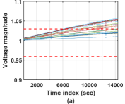
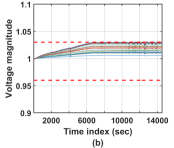
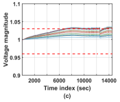
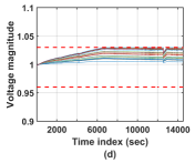
For Algorithm 2, we adopt a step-size $\eta_{t}=0.01/\sqrt{t}$. Figure 1 showcases the voltage levels at PES buses throughout the online identification and distributed control process, updating the model in real-time as new input-output data becomes available. Figure 1(a) illustrates potential violations of voltage regulation limits without control measures. Figure 1(b) depicts the outcomes using distributed control based on the LinDistFlow model. The real-time estimated linear model closely approximates the LinDistFlow model, reflected a satisfactory control performance in Figure 1(c), albeit with some fluctuations during periods of reduced PES generation. Notably, the control performance using the identified non-linear model, as shown in Figure 1(d), surpasses that of the linear model, which aligns with expectations given the non-linear model’s closer representation of actual power flow dynamics. Overall, the models identified through our proposed algorithm demonstrate effective voltage regulation capabilities.

Refer to caption
(a)
Refer to caption
(b)
Refer to caption
(c)
Refer to caption
(d)
Figure 1: The voltage magnitudes ($p.u.$) over time (a) without any control (b) with distributed feedback-based control and the LinDistFlow, [11] model (c) with online distributed estimated linear power flow model and feedback-based control (d) with online distributed estimated non-linear power flow model and feedback-based control.

V Conclusion

In this paper, we developed an online distributed algorithm where each agent updates its estimate of the model via an online gradient descent scheme utilizing the most recent input-output pair. We prove that the developed distributed algorithm has a sub-linear regret and determines the original system model. The real-time updates of the agents, utilizing sequential data, significantly reduce the communication network’s bandwidth requirements. Further, agents only share non-linear estimates preserving their private information. The numerical simulation study corroborates the efficacy of our developed algorithm with the identification of a more accurate quadratic power flow model, which improves the voltage regulation performance of the control system.

References

  • [1] Y. Liao, Y. Weng, G. Liu, and R. Rajagopal, “Urban MV and LV distribution grid topology estimation via group lasso,” IEEE Transactions on Power Systems, vol. 34, no. 1, pp. 12–27, 2018.
  • [2] O. Ardakanian, V. W. Wong, R. Dobbe, S. H. Low, A. von Meier, C. J. Tomlin, and Y. Yuan, “On identification of distribution grids,” IEEE Transactions on Control of Network Systems, vol. 6, no. 3, pp. 950–960, 2019.
  • [3] J. Yu, Y. Weng, and R. Rajagopal, “PaToPa: A data-driven parameter and topology joint estimation framework in distribution grids,” IEEE Transactions on Power Systems, vol. 33, no. 4, pp. 4335–4347, 2017.
  • [4] J. Zhang, P. Wang, and N. Zhang, “Distribution network admittance matrix estimation with linear regression,” IEEE Transactions on Power Systems, vol. 36, no. 5, pp. 4896–4899, 2021.
  • [5] S. D. McArthur, E. M. Davidson, V. M. Catterson, A. L. Dimeas, N. D. Hatziargyriou, F. Ponci, and T. Funabashi, “Multi-agent systems for power engineering applications—part i: Concepts, approaches, and technical challenges,” IEEE Transactions on Power systems, vol. 22, no. 4, pp. 1743–1752, 2007.
  • [6] O. P. Mahela, M. Khosravy, N. Gupta, B. Khan, H. H. Alhelou, R. Mahla, N. Patel, and P. Siano, “Comprehensive overview of multi-agent systems for controlling smart grids,” CSEE Journal of Power and Energy Systems, vol. 8, no. 1, pp. 115–131, 2020.
  • [7] C.-Y. Chang, “A privacy preserving distributed model identification algorithm for power distribution systems,” in 62nd IEEE Conference on Decision and Control, 2023.
  • [8] D. E. Knuth, The Art of Computer Programming, Volume 1: Fundamental Algorithms.   Addison-Wesley, 1997.
  • [9] Y. Huang, Z. Meng, and J. Sun, “Scalable distributed least square algorithms for large-scale linear equations via an optimization approach,” Automatica, vol. 146, p. 110572, 2022.
  • [10] C.-Y. Chang, M. Colombino, J. Cortés, and E. Dall’Anese, “Saddle-flow dynamics for distributed feedback-based optimization,” IEEE Control Systems Letters, 2019.
  • [11] M. E. Baran and F. F. Wu, “Network reconfiguration in distribution systems for loss reduction and load balancing,” IEEE Transactions on Power delivery, vol. 4, no. 2, pp. 1401–1407, 1989.