Robustness of graph embedding methods for community detection

Abstract

This study investigates the robustness of graph embedding methods for community detection in the face of network perturbations, specifically edge deletions. Graph embedding techniques, which represent nodes as low-dimensional vectors, are widely used for various graph machine learning tasks due to their ability to capture structural properties of networks effectively. However, the impact of perturbations on the performance of these methods remains relatively understudied. The research considers state-of-the-art graph embedding methods from two families: matrix factorization (e.g., LE, LLE, HOPE, M-NMF) and random walk-based (e.g., DeepWalk, LINE, node2vec). Through experiments conducted on both synthetic and real-world networks, the study reveals varying degrees of robustness within each family of graph embedding methods. The robustness is found to be influenced by factors such as network size, initial community partition strength, and the type of perturbation. Notably, node2vec and LLE consistently demonstrate higher robustness for community detection across different scenarios, including networks with degree and community size heterogeneity. These findings highlight the importance of selecting an appropriate graph embedding method based on the specific characteristics of the network and the task at hand, particularly in scenarios where robustness to perturbations is crucial.

I Introduction

The use of low-dimensional vector representations, or graph embeddings, has garnered significant attention across various disciplines [1, 2, 3]. These representations play a crucial role in characterizing important functional network properties such as robustness and navigability [4, 5, 6, 7]. Additionally, they are instrumental in performing graph analysis tasks including node classification [8], link prediction [9], and visualization [10].

Communities, which are sets of nodes more likely to be connected to each other than to the rest of the graph, are fundamental features of many complex systems represented as graphs [11, 12, 13]. Recent research has demonstrated the potential of using graph embeddings for community detection in networks [14]. This approach leverages the inherent structural information captured in the vector representations to identify cohesive groups of nodes within the network. Overall, graph embeddings offer a versatile framework for analyzing and understanding complex networks, enabling a wide range of applications across various domains.

Community detection using graph embeddings relies on representing graph nodes as points in a low-dimensional vector space, where communities manifest as clusters of points that are close to each other and sufficiently separated from other clusters [14, 15, 16]. These clusters are then recovered using standard data clustering techniques such as $k$-means clustering [17]. Given the practical importance of consistently detecting communities and the effectiveness of graph embedding approaches in doing so, it is essential to investigate the robustness of graph embeddings for community detection under network perturbations. In this context, robustness refers to the ability of a graph embedding method to tolerate perturbations while still accurately recovering the original community structure [18, 19, 20]. This investigation is crucial for understanding how communities identified by graph embedding methods withstand random errors or adversarial attacks, serving as a proxy for evaluating network functionality. Robust graph embeddings ensure the reliability and stability of community detection algorithms in real-world network applications.

Previous research has investigated the impact of network perturbations on the robustness of community structures, focusing on techniques that characterize structural properties of communities such as internal link density [21, 20]. However, little attention has been given to understanding the robustness of graph embedding methods used for community detection under perturbations in the graph topology. While there are numerous graph embedding techniques available for community detection [1, 22], it remains challenging for practitioners to select a robust method and comprehend its implications across various factors, including the size of the network, strength of the original community structure, type of perturbation, and the specific embedding technique used. Moreover, the majority of research on using graph embeddings for community detection has been conducted on synthetic networks, warranting validation of the effects of perturbations on real-world network data. Addressing these gaps in research, we aim to investigate the robustness of graph embedding methods for community detection under different types of perturbations in the graph topology. By exploring these factors across synthetic and real-world network datasets, we seek to provide insights into the effectiveness and limitations of graph embedding techniques in preserving community structures amidst network perturbations.

In this paper, we address this gap of knowledge by devising a systematic framework to investigate the robustness of graph embedding methods used to extract community structures under network perturbations. We consider both synthetic Lancichinetti-Fortunato-Radicchi (LFR) benchmark graphs [23] and empirical networks with degree and community size heterogeneity. Our perturbation approach involves the removal of edges based on random node selection [21] and targeted node selection using betweeness centrality [24, 25, 26]. We use seven state-of-the-art graph embedding methods, namely Laplacian eigenmap (LE) [27], locally linear embedding (LLE) [28], higher-order preserving embedding (HOPE) [29], modularized non-negative matrix factorization (M-NMF) [30] in the matrix factorization family; and DeepWalk [31], large-scale information network (LINE) [32], and node2vec [33] in the random walk family. We use $k$-means based on spherical distance [34] to achieve more effective clustering results in high-dimensional spaces. We use element-centric similarity (ECS) [35], a widely adopted community similarity metric, to quantify changes in the similarity partitions after many realizations with perturbations as a proxy of characterizing graph embedding robustness. This comprehensive methodology allows us to systematically assess and compare the impact of various perturbation strategies on the robustness of graph embedding methods for community detection in both synthetic and real-world networks.

Our findings indicate that incremental selection of nodes and subsequent removal of their adjacent edges consistently reduce ECS. However, this impact tends to be more noticeable across graph embedding methods, but node2vec and LLE, and varies across network sizes, the initial community structure strength, and the perturbation type. This aligns with the expectation that removing a greater number of edge results in a more substantial disruption of the community structure. Notably, targeted node selection leads to a more pronounced and accelerated decline in ECS compared to random node selection. This is rationalized by the fact that adversarial attacks tend to swiftly dismantle the network’s community structure. Among the seven network embedding methods considered, node2vec and LLE consistently demonstrate to be more robust for community detection within their respective graph embedding families. Overall, node2vec is the most robust graph embedding method for community detection. Our results generally concur with those of Kojaku et al. [16], which found that node2vec learns more consistent community structures with networks of heterogeneous degree distributions and size.

We have made available the code to reproduce all the results at .

II Methods

II.1 LFR benchmark

Lancichinetti–Fortunato–Radicchi (LFR) benchmark graphs [23, 37] have become a widely adopted tool for generating graphs with ground-truth communities. One of the primary advantages of utilizing the LFR benchmark is its ability to produce graphs where both degree and community size distributions follow power-law distributions. These distributions closely resemble the properties observed in many real-world networks [23, 38, 39, 40]. The exponents governing the degree and community size distributions are controlled by the parameters $\alpha$ and $\beta$, respectively. To generate LFR benchmark graphs, one must specify various other parameters, including the average degree $\langle k\rangle$, maximum degree $maxk$, minimum community size $minc$, maximum community size $maxc$, and the mixing parameter $\mu$. The mixing parameter $\mu$ represents the fraction of nodes that share edges across different communities, with lower values of $\mu$ leading to a higher ratio between internal and external edges. This results in increased modularity, a commonly used quality metric for assessing community strength in community research [11]. Thus, smaller values of $\mu$ correspond to stronger partitions. Note that LFR benchmark graphs are undirected and unweighted.

We generate LFR benchmark graphs using the LFR_benchmark_graph method in the publicly available Python package NetworkX [41]. Our experiments involve two different network sizes: $1,000$ nodes and $10,000$ nodes, allowing us to investigate the impact of perturbations at varying scales. Furthermore, we explore the influence of the initial community strength by adjusting the mixing parameter, $\mu$. The specific parameter values utilized for the generation of LFR benchmark graphs are detailed in Table 1. Note that the proposed experimental design can be applied to any other synthetic graph generators such as the Girvan–Newman benchmark [42] and the stochastic block model [43].

Table 1: Synthetic experiment parameters.

Parameter	Description	Value
$N$	number of nodes	$1,000$ and $10,000$
$maxk$	max degree for LFR	$0.1N$
$\langle k\rangle$	average degree for LFR	$25$
$maxc$	max community size for LFR	$0.1N$
$\alpha$	degree distribution exponent for LFR	$-2$
$\beta$	community size distribution exponent for LFR	$-1.1$
$\mu$	mixing parameter for LFR	$0.01,0.1,0.2,0.3,0.4,0.5$
$r$	number of realizations	$50$

II.2 Edge removal procedure

Our edge removal procedure investigates the impact of eliminating edges in the network structure. We employ two distinct methods: edge removal based on random node selection and edge removal based on targeted node selection.

Let’s first discuss edge removal based on random node selection. This simulates random network errors in real-world scenarios [44, 45]. We do so by selecting $p\%$ of nodes randomly and deleting their adjacent edges. To make our experiment unbiased, we independently generate $50$ distinct sets of nodes. In other words, the number of realizations is $r=50$ (see Table 1). We ensure that the removal of edges from each set of nodes does not disconnect the remaining part of the network, which is required by the graph embedding methods. In the event that the remaining part of the network becomes disconnected after the removal of a set of edges, we omit this set of nodes and proceed with re-sampling. After each removal, we measure the similarity between the community structure of the remaining network in the embedding space calculated using data clustering (i.e., $k$-means; see more details in Sec. II.3) and the community structure of the original LFR network using community similarity metrics (i.e., ECS [35]) as detailed in Sec. II.4. The overall similarity score for a given $p\%$ value is calculated by averaging the similarity scores across all $50$ sets.

Second, we discuss targeted edge removal. Targeted edge removal is based on the betweenness centrality of nodes. Betweenness centrality measures the importance of a node in a network based on how often it lies on the shortest paths between other nodes [46]. Node with high betweenness centrality usually indicate nodes of vital importance to the network, so removing edges adjacent to these nodes might cripple the functionality of the network [47]. This approach models an adversarial attack in real-world situations [48, 49]. To implement edge removal based on targeted node selection, we first rank the nodes in the network by their betweenness centrality. The node with the lowest betweenness centrality has rank $1$, and the node with the highest betweenness centrality has rank $N$, where $N$ is the number of nodes in the network. We then independently generate $50$ sets of nodes, each containing $p\%$ of nodes in the network. The nodes in each set are selected by randomly sampling nodes with probability proportional to their betweenness centrality rank. We ensure that the removal of edges adjacent to each set of nodes does not disconnect the remaining part of the network, which is required by graph embedding methods. In the event that the remaining part of the network becomes disconnected after the removal of a set of edges, we omit the set of nodes and proceed with re-sampling. After each removal, we measure the similarity between the community structure of remaining network in the embedding space computed through data clustering (i.e., $k$-means; see more details in Sec. II.3) and the ground-truth community structure of the original LFR network using ECS. The overall similarity score for a given $p\%$ is calculated by averaging community similarity scores across all $50$ sets.

In our experiments, the proportion of selected nodes starts from $5\%$ with an increment of $5\%$. The upper bound of proportion depends on the network structure and the node selection method. For example, when we select a network with $N=1,000$, $\mu=0.01$, and use edge removal based on targeted node selection, it is difficult to keep the network connected when deleting edges adjacent to $35\%$ of nodes. In these cases, we use a proportion of selected nodes that is below the threshold, e.g., $5\%$, $10\%$, $15\%$, $20\%$, $25\%$, and $30\%$. In addition, we also perform data clustering on the embeddings of the original LFR networks with no edges removed and compare the results with the ground-truth community structure. This result will be recorded as “0% of nodes selected.” We also capture the variation of the measurements by computing standard deviations. As the standard deviations are negligible with respect to the mean, we do not show those results here.

II.3 Data clustering

Community detection (or clustering) is the task of grouping nodes in a network based on their connectivity. A general consensus is that nodes within the same community are more densely connected than nodes across different communities. There are many different community detection algorithms, each with its own strengths and weaknesses [14]. The best algorithm for a particular network depends on the properties of the network and performance constraints [50].

In this article, we perform community detection based on a two-step process consisting of graph embedding [22] and the $k$-means algorithm [51] for data clustering. That is, we control the data clustering step by using the $k$-means method to optimally find the clusters in the low-dimensional representation. Specifically, we perform graph embedding to assign a point in the Euclidean space to each node in the network. Here, we focus on embedding each node of the graph rather than the whole graph (more details on node-embedding methods can be found in [52]). We use seven state-of-the-art graph embedding methods studied in previous research [14] across two different families of graph embedding methods, including: (1) matrix-based methods and (2) random walk methods (according to the taxonomy by M. Xu in [22]). In the matrix-based family, we include Laplacian eigenmap (LE) [27], locally linear embedding (LLE) [28], higher-order preserving embedding (HOPE) [29], and modularized non-negative matrix factorization (M-NMF) [19]. In the random walk family, we include DeepWalk [31], large-scale information network (LINE) [32], and node2vec [33]. Note that we make the distinction between graph embedding families to stress the foundational mechanism under which graph embeddings are constructed. We, however, note that under specific conditions regarding the window size of the skip-gram model, random walk methods are equivalent to matrix factorization methods [53]. Tandon et. al provides a thorough test on graph embedding methods for data clustering, which have been shown to perform well for community detection in networks [14].

We use the publicly available Python package nxt_gem for LE and HOPE [54]. As there is no correct implementation of LLE for graphs available online, we developed our own implementation available on GitHub in . The package karateclub includes implementations of DeepWalk and M-NMF [56]. The package GraphEmbedding for LINE is publicly available on GitHub in . We utilize node2vec package for node2vec embedding available online .

After computing graph embeddings, we use the $k$-means algorithm to group the points in the Euclidean space into clusters. Note that other data clustering algorithms used before to cluster embedding results, such as Gaussian mixture models [59], lead to similar results as $k$-means [14]. The $k$-means algorithm, a popular method in data clustering, minimizes the distance between each data point and its centroid. It works by iteratively assigning data points to the nearest cluster centroid and then updating the centroids based on the average of the assigned points until convergence, aiming to minimize the within-cluster variance. In our case, the data points are the embedding points in Euclidean space for each network node and centroids are virtual points representing the clusters. As in high-dimensional spaces, the concept of proximity may not be meaningful as different distances may select different neighbors for the same point [60]; we use $k$-means based on spherical distance to get better clustering outcome. According to [34], $k$-means based on spherical distance is a widely used clustering algorithm for sparse and high-dimensional data. Specifically, for two nodes embedded as points $\mathbf{x}=(x_{1},x_{2},\ldots,x_{d})$ and $\mathbf{y}=(y_{1},y_{2},\ldots,y_{d})$ in the $d$-dimensional Euclidean space, the spherical distance between the two nodes is defined as

$$\mathsf{d}_{S}(\mathbf{x},\mathbf{y})=1-\frac{\sum_{i=1}^{d}x_{i}y_{i}}{\sqrt{\sum_{i=1}^{d}x_{i}^{2}\sum_{i=1}^{d}y_{i}^{2}}}.$$

As data clustering methods often necessitate prior knowledge of the number of clusters, we provide the data clustering procedure with the correct number of clusters derived from the LFR benchmark graphs. By doing so, we ensure a fair evaluation of the embedding methods. Note that such a luxury may be absent when analyzing real-world networks, as the true number of clusters is typically unknown in those cases.

II.4 Community similarity

To measure the similarity between community partitions, we employ ECS [35], computed with the CluSim package [61]. Compared to other clustering similarity metrics such as the normalized mutual information (NMI) [62], ECS is a most robust metric for comparing clusters and better addresses challenges such as biases in randomized membership, skewed cluster sizes, and the problem of matching [35]. We use default parameter values in ECS computation.

ECS yield values in the range from $0$ to $1$, where a higher value indicates a greater similarity between partitions.

Fig. 1 is a schematic diagram showing the process we follow in our experimental design.

Figure 1: Schematic diagram of experimental design.

III Results and Discussion

In this section, we present the results of our experiments. Recall that Sec. II.3 details the embedding methods we use here. In the following subsections, we use $\mathbf{A}$ to denote the adjacency matrix of a graph. We report results based on the family of graph embedding methods (i.e., matrix-based family in Sec. III.1 and random walk family in Sec. III.2).

In the subsequent line figures, unless otherwise stated, subfigures in the top row, i.e., (a) and (b), correspond to random node selection. More specifically, subfigure (a) corresponds to $16$-dimensional embeddings and subfigure (b) depicts results obtained with $32$-dimensional embeddings. Similarly, subfigures in the bottom row, i.e., (c) and (d), correspond to targeted node selection. More specifically, subfigure (c) corresponds to $16$-dimensional embeddings and subfigure (d) depicts results obtained with $32$-dimensional embeddings. We focus only in these two dimensions as smaller embedding dimensions seem to be enough to provide an accurate low-dimensional vector representation of networks [15, 16]. Recall that a higher ECS value indicates a greater similarity between network community partitions obtained from the LFR benchmark graphs and the embeddings. Thus, when analyzing line figures, higher ECS values and therefore higher positions of line curves indicate a more robust graph embedding method for community detection.

In addition, to facilitate a thorough comparison of embedding methods, heatmaps are employed to offer a more comprehensive assessment on the joint effect of network size and embedding dimension in community robustness for a fixed $\mu$ in absence of perturbations. Specifically, for different community partition strengths (i.e., strong with $\mu=0.01$ and weak with $\mu=0.5$), $50$ independent instances of LFR networks are generated, each with a distinct network size. The identified community structures, with different embedding dimensions, are then compared with the ground-truth community partition using the ECS similarity score. The mean similarity score derived from $50$ copies of LFR networks is utilized to populate each cell in the heatmap. When producing heatmaps, we notice that the standard deviations are negligible with respect to the mean; so, we do not show those results. Note that no edge removal is involved in drawing heatmaps.

Table 2: Parameter values for embedding methods.

Family	Method	Parameters
Matrix	HOPE	$\beta=0.01$
Matrix	M-NMF	$\lambda=0.2$, $\alpha=\beta=0.05$, $\eta=5$, $N=200$
Random Walk	DeepWalk	$t=40$, $w=10$, $n=80$
Random Walk	LINE	batch size: $8192$, epochs: $100$
Random Walk	node2vec	$t=10$, $w=10$, $n=80$, $p=q=1$

Table 2 shows the experimental parameters employed by the embedding methods, excluding embedding dimensions, $d$. Notably, LE and LLE methods only require the embedding dimension $d$. For the remaining parameters, we utilized the default parameters as specified in Tandon et al. (2021) [14]; they show that default values of parameters for the embedding methods lead to comparable performance as traditional community detection methods, and that the optimized parameters do not exhibit a significant improvement over default parameters.

In Sec. III.3, we conduct cross-comparisons between data clustering methods using heatmaps, to compare how similar are the community detection outcomes based on various embedding techniques. We observe that LE and LLE, as two methods in the family of matrix-based methods, yield similar data clustering results; similarly, DeepWalk and node2vec, as two methods in the family of random walk-based approaches, also exhibit similar results.

Finally, Sec. III.4 presents experimental results to evaluate the robustness of our community detection methods on two real-world networks with labeled communities: the email-EU-core network [63] and the AS network [7]. These networks exhibit similar characteristics to synthetic counterparts, specifically power-law degree and community size distributions as observed in LFR benchmark graphs. Our experimental methodology and insights for real-world networks mirrors previous findings for synthetic counterparts.

III.1 Matrix factorization methods

Matrix-based methods project network nodes onto a Euclidean space via eigenvectors following a similar idea as in spectral clustering [64]. In this family of methods, we include Laplacian eigenmap (LE) [1, 27], locally linear embedding (LLE) [14, 28], higher-order preserving embedding (HOPE) [1, 29], and modularized non-negative matrix factorization (M-NMF) [14, 19]. We now detail results in each of them.

III.1.1 Laplacian eigenmap (LE)

Laplacian eigenmap (LE) [1, 27] aims to minimize the objective function

$$\sum_{i,j}\left|\mathbf{x}_{i}-\mathbf{x}_{j}\right|^{2}\mathbf{A}_{ij},$$

subject to the constraint $\mathbf{x}^{T}\mathbf{D}\mathbf{x}=\mathbf{I}$, where $\mathbf{D}$ represents the diagonal matrix of graph node degrees, and $\mathbf{x}_{i}$ denotes the vector indicating the position of the point representing node $i$ in the embedding. For $d$-dimensional embedding with LE, the solution can be obtained by extracting the eigenvectors corresponding to the $d$ smallest eigenvalues (except the zero eigenvalue) of the normalized Laplacian matrix

$$\mathbf{D}^{-1}(\mathbf{D}-\mathbf{A})$$

In Figs. 2 and 3, the impact of edge removal based on different node selection strategy is demonstrated. The effects of the initial community partition’s strength (with stronger partitions experiencing less perturbation impact, i.e., lower $\mu$ values) and the type of perturbation (targeted node selection having a significant influence on clusters) are observed. Specifically, for networks with strong community partition (i.e., $\mu=0.01$ or $\mu=0.1$), we notice that embedding dimension tends to have a stronger effect on the decay rate of similarity, despite node selection strategy. For instance, in Fig. 2(a), with an embedding dimension of $16$, the curve corresponding to $\mu=0.1$ remains consistently stable around an ECS value of approximately $1.0$ until $60\%$ of nodes are selected. Subsequently, between $60\%$ and $85\%$ of nodes selected, the curve gradually and steadily decreases from $1.0$ to $0.84$ (i.e., $16\%$ decrease). In contrast, depicted in Fig. 2(b) with an embedding dimension of $32$, the curve representing $\mu=0.1$ remains stable around $1.0$ only until $25\%$ of node are selected. Then, between $25\%$ and $85\%$ of nodes selected, the curve decreases more sharply from $1.0$ to $0.53$ (i.e., $47\%$ decrease).

Fig. 4 helps us to better understand the effect of embedding dimension and network size. We notice that for strongly clustered networks (i.e., $\mu=0.01$), a lower embedding dimension produces higher ECS. On the contrary, for weakly clustered networks (i.e., $\mu=0.5$), lower embedding dimensions produce higher ECS for networks with small sizes and higher embedding dimensions result in higher ECS for networks with larger sizes. In both scenarios represented by Fig. 4(a) and Fig. 4(b), it is observed that, for a given fixed embedding dimension, the data clustering method employing LE yields higher ECS scores for larger networks.

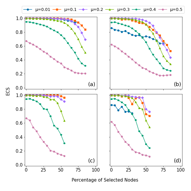
Figure 2: Mean ECS using LE method over the percentage of selected nodes on LFR benchmark graphs with $1,000$ nodes. (a) and (b) use random node selection while (c) and (d) use targeted node selection.

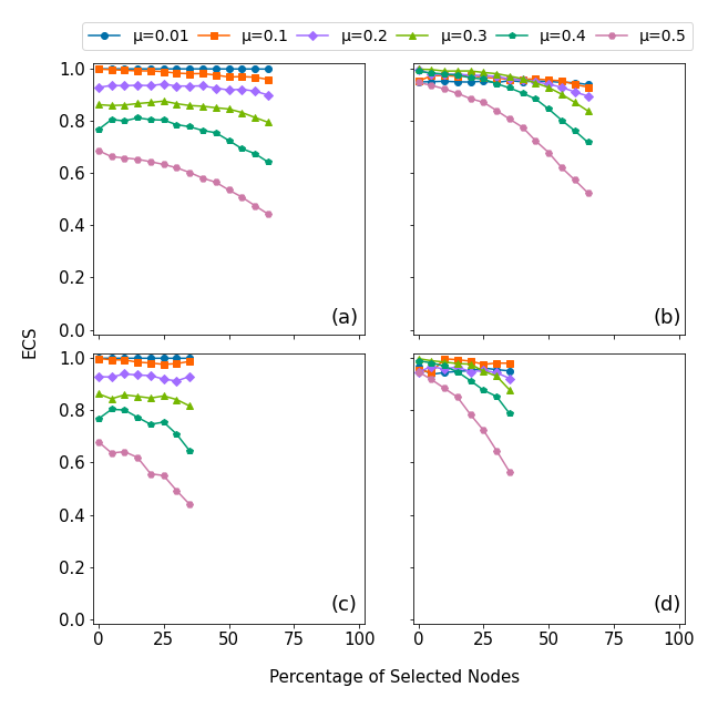
Figure 3: Mean ECS using LE method over the percentage of selected nodes on LFR benchmark graphs with $10,000$ nodes. (a) and (b) use random node selection while (c) and (d) use targeted node selection.

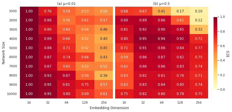
Figure 4: Heatmaps with LE embedding method. For given embedding dimension and LFR network with given size, the ECS similarity score between ground-truth community structure and detected community structure is recorded.

III.1.2 Locally linear embedding (LLE)

Locally linear embedding (LLE) [14, 28] minimizes the objective function

$$\sum_{i}\Bigl{|}\mathbf{x}_{i}-\sum_{j}\mathbf{A}_{ij}\mathbf{x}_{j}\Bigr{|}^{2}.$$

Given the form of the objective function, each point in the embedded space $\mathbf{x}_{i}$ is approximated as a linear combination of its neighbors in the original graph. To ensure a well-posed problem, solutions are required to be centered at the origin, i.e., $\sum_{i}\mathbf{x}_{i}=0$, and to have unit variance, i.e., $\frac{1}{N}\mathbf{x}^{T}\mathbf{x}=\mathbf{I}$. Subject to these constraints, for a $d$-dimensional embedding with LLE, the solution is approximated by the eigenvectors corresponding to the lowest $d$ eigenvalues (excluding the zero eigenvalue) of the matrix $(\mathbf{I}-\mathbf{A})^{T}(\mathbf{I}-\mathbf{A})$.

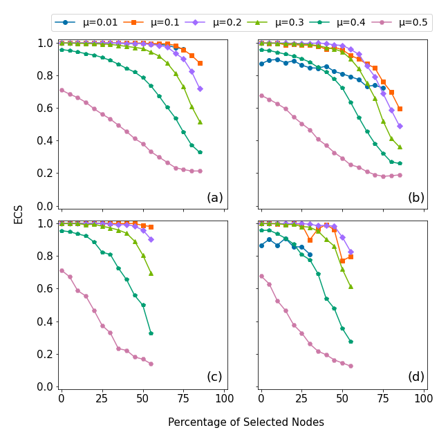
Figure 5: Mean ECS using LLE method over the percentage of selected nodes on LFR benchmark graphs with $1,000$ nodes. (a) and (b) use random node selection while (c) and (d) use targeted node selection.

The insights drawn from Figs. 5, 6 and 7 for LLE align closely with the insights derived for LE.

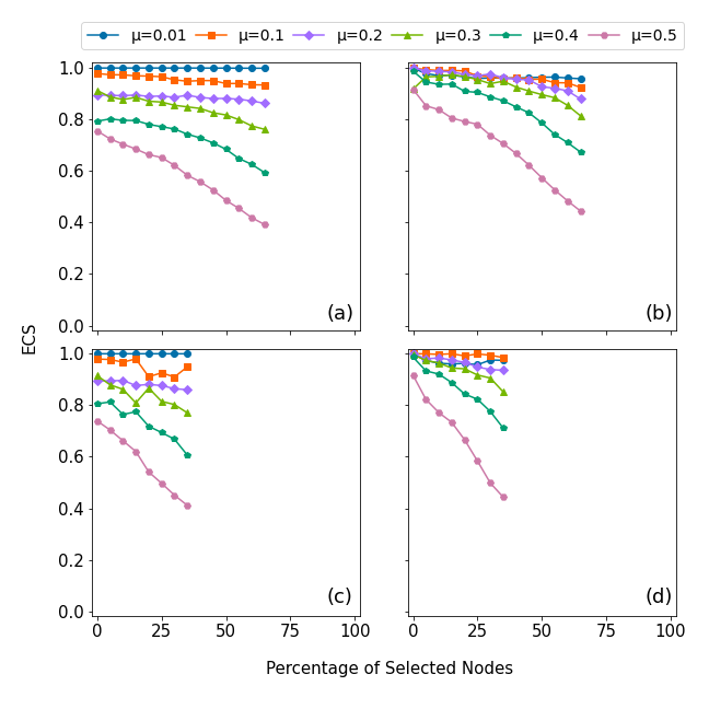
Figure 6: Mean ECS using LLE method over the percentage of selected nodes on LFR benchmark graphs with $10,000$ nodes. (a) and (b) use random node selection while (c) and (d) use targeted node selection.

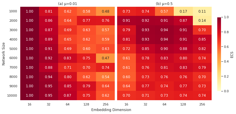
Figure 7: Heatmaps with LLE embedding method. For given embedding dimension and LFR network with given size, the ECS similarity score between ground-truth community structure and detected community structure is recorded.

III.1.3 Higher-order preserving embedding (HOPE)

Higher-order preserving embedding (HOPE) is designed to maintain the similarity between nodes [1, 29]. The objective function being optimized is $\bigl{|}\mathbf{S}-\mathbf{x}\mathbf{x}^{T}\bigr{|}$, where $\mathbf{S}$ is the Katz similarity matrix defined as

$$\mathbf{S}=\beta\sum_{\ell=1}^{\infty}\mathbf{A}^{\ell},$$

with $\beta$ denoting the decay parameter. In our experiments, we set $\beta=0.01$.

Our experimental results on the impact of edge removal, generated through the HOPE embedding method, are presented in Figs. 8 and 9. For the HOPE embedding method, our results suggest that using a 32-dimensional embedding (i.e., subfigures (b) and (d) in the right panel) brings higher ECS scores than a 16-dimensional one (i.e., subfigures (a) and (c) in the left panel). We can also see that HOPE has higher ECS scores with smaller graphs. Analysis of heatmaps in Fig. 10 reveals that the HOPE method tends to preserve effectively higher ECS scores for smaller networks and higher embedding dimensions.

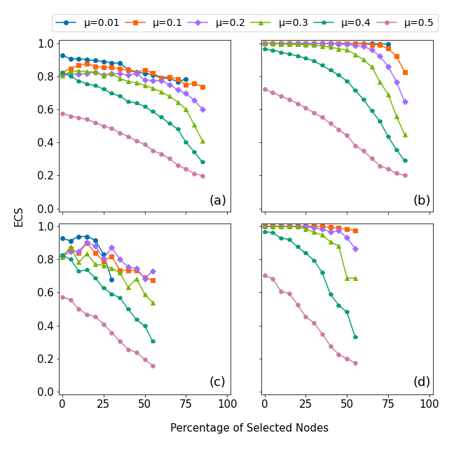
Figure 8: Mean ECS using HOPE method over the percentage of selected nodes on LFR benchmark graphs with $1,000$ nodes. (a) and (b) use random node selection while (c) and (d) use targeted node selection.

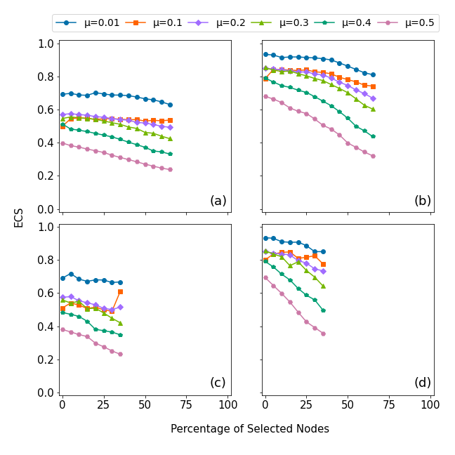
Figure 9: Mean ECS using HOPE method over the percentage of selected nodes on LFR benchmark graphs with $10,000$ nodes. (a) and (b) use random node selection while (c) and (d) use targeted node selection.

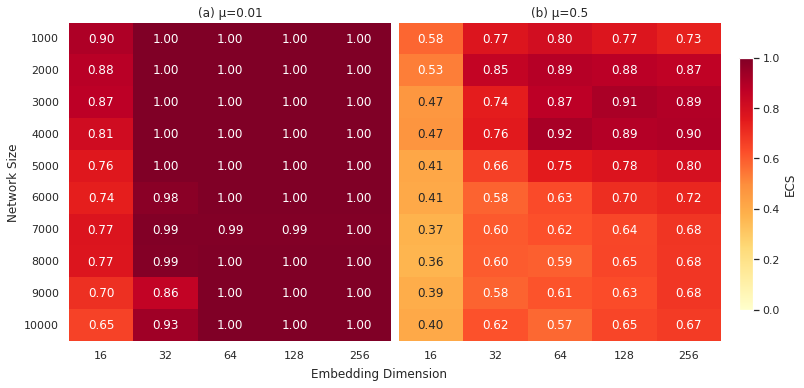
Figure 10: Heatmaps with HOPE embedding method. For given embedding dimension and LFR network with given size, the ECS similarity score between ground-truth community structure and detected community structure is recorded.

III.1.4 Modularized non-negative matrix factorization (M-NMF)

Modularized Non-Negative Matrix Factorization (M-NMF) [19] preserves both the first-order proximity (pairwise node similarity) and the community structure for network embedding. Modularity, which evaluates the quality of community partitions within a network by comparing the observed network with randomized versions that lack inherent community structure, is integrated into the optimization function of M-NMF. While minimizing the optimization function of M-NMF (see [19]), nodes are brought into proximity when they exhibit similarity and simultaneously when they are part of clusters derived from high-modularity partitions [14].

The following parameter values are used in our experiments: $\lambda=0.2$, $\alpha=0.05$, $\beta=0.05$, $\eta=5.0$, and number of iterations $N=200$. Our experimental results on the impact of edge removal, generated through the M-NMF embedding method, are reported in Figs. 11 and 12. From these figures, we can see that M-NMF produces higher ECS scores with smaller graphs. Reviewing heatmaps in Fig. 13, M-NMF produces higher ECS scores for strongly clustered networks, but a clear pattern is not discernible. Notably, from Fig. 13(b), M-NMF produces lower ECS scores in cases where $\mu=0.5$. Recall that M-NMF tries to preserve the community structure of networks and therefore is strongly affected by perturbations when the initial community structure is weak.

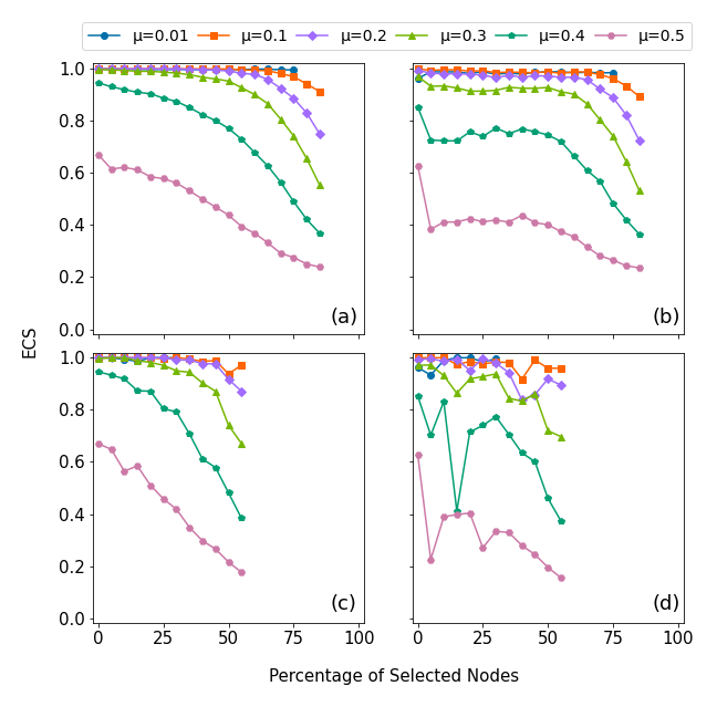
Figure 11: Mean ECS using M-NMF method over the percentage of selected nodes on LFR benchmark graphs with $1,000$ nodes. (a) and (b) use random node selection while (c) and (d) use targeted node selection.

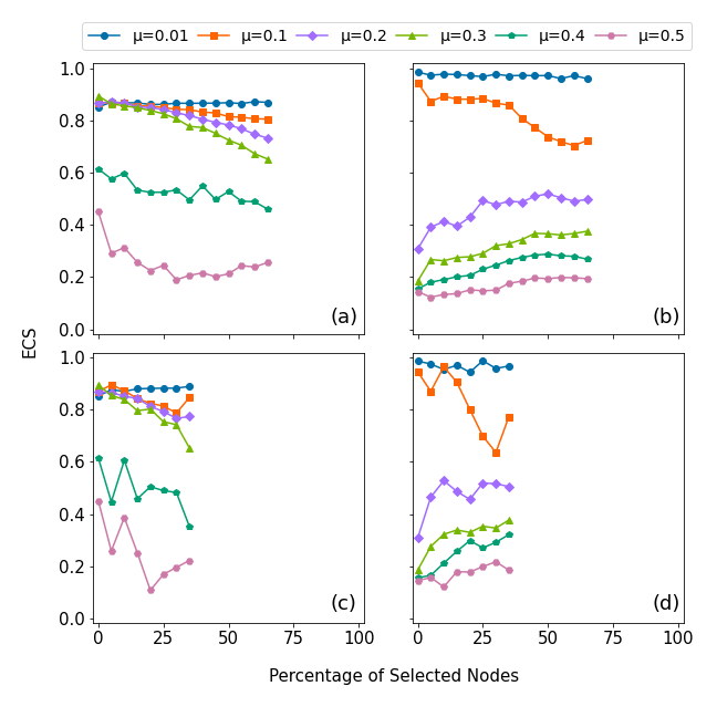
Figure 12: Mean ECS using M-NMF method over the percentage of selected nodes on LFR benchmark graphs with $10,000$ nodes. (a) and (b) use random node selection while (c) and (d) use targeted node selection.

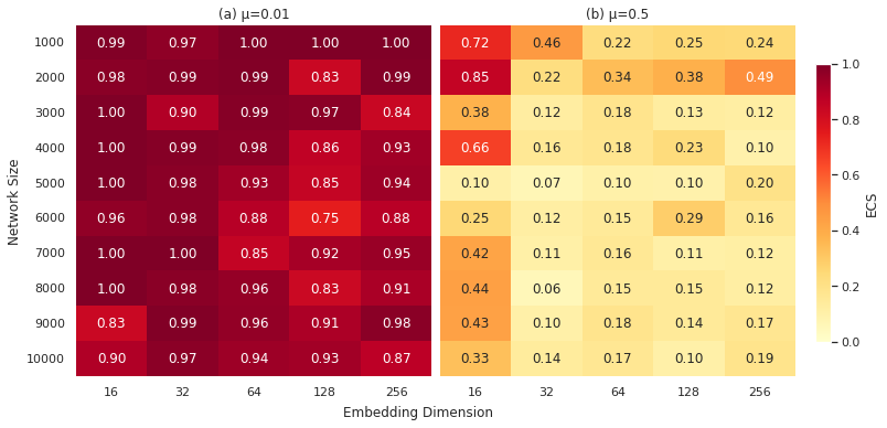
Figure 13: Heatmaps with M-NMF embedding method. For given embedding dimension and LFR network with given size, the ECS similarity score between ground-truth community structure and detected community structure is recorded.

Table 3: Choice of more robust graph embedding methods in the family of matrix-factorization.

	Weaker Community Structure (larger $\mu$)	Stronger Community Structure (smaller $\mu$)
Smaller Network (smaller $N$)	LLE with a low embedding dimension	LLE with a low embedding dimension, or HOPE with a high embedding dimension
Larger Network (larger $N$)	LE with a higher embedding dimension	LE with a lower embedding dimension

We derive the following insights for matrix factorization methods. In a nutshell, we observe that ECS scores consistently decrease as we progressively select more nodes and delete their adjacent edges and the networks become sparser. This aligns with our intuition that the community structure is more significantly disrupted when a greater number of edges are removed. From previous figures, it is evident that, in general, for smaller values of $\mu$, the ECS similarity score tends to remain higher for varying degrees of perturbations. This suggests that the graph embedding methods tend to produce higher ECS scores when the original LFR benchmark graph exhibits a stronger partition. Recall that $\mu$ signifies the fraction of nodes sharing edges across different communities. Thus, a lower $\mu$ value implies a higher ratio of internal to external edges, usually resulting in a more pronounced partition in the LFR benchmark graph. Notably, when utilizing targeted node selection, the ECS exhibits a more pronounced and rapid decline compared to random selection. For example, for LFR network with $1,000$ nodes and $\mu=0.5$, when perturbing the network at $50\%$ and using LE with $16$-dimensional embedding, we notice that targeted node selection decreases ECS from $0.67$ to $0.14$ (a decrease of $79.1\%$, see Fig. 2(c)), but ECS decreases from $0.67$ to $0.35$ for random node selection (a decrease of $47.8\%$, see Fig. 2(a)). This observation is comprehensible, as targeted node selection based on betweenness centrality tend to dismantle the network’s community structure more swiftly.

For smaller real-world graphs containing a few thousand vertices, to obtain more robust partitions, the LLE method is suggested with a modest embedding dimension, typically on the order of tens, such as 16 dimensions in our experiments. Alternatively, when the community partition is stronger, the HOPE embedding method with a higher embedding dimension produces more robust partitions. In the case of larger real-world graphs with a weaker community partition, to obtain more robust community partitions, it is suggested to use the LE embedding method with a moderately higher embedding dimension, such as $32$ or $64$ dimensions, as utilized in our experiments. When dealing with larger real-world graphs characterized by a stronger community structure, the LE embedding method with a lower embedding dimension produces more robust community partitions. Alternatively, achieving comparable results can also be accomplished by employing the LLE embedding method with a lower embedding dimension.

III.2 Random walk methods

Random walk methods learns network embeddings of graph nodes by modeling a stream of short random walks. We chose DeepWalk [31], LINE [32], and node2vec [33], as widely used methods of this family.

III.2.1 DeepWalk

DeepWalk [31] extends language modeling techniques to graphs, departing from words and sentences. This algorithm leverages local information acquired through random walks, treating these walks as analogous to sentences in the word2vec [65] language modeling approach. To generate a random walk originating from a specified starting node, neighbors of the current node in the walk are randomly selected and added to the walk iteratively until the intended walk length is achieved. In our experiments, we use the following parameters: random walk length $t=40$, window size $w=10$, number of walks per node $n=80$.

Our experimental results on the impact of edge removal, generated through the DeepWalk embedding method, are reported in Figs. 14 and 15. We can observe that networks with stronger initial partitions (i.e., lower $\mu$ values) experience less perturbation impact and targeted node selection has a significant influence on clusters. Examining heatmaps in Fig. 16(a), it is evident that for strongly clustered networks, the DeepWalk embedding method produces higher ECS scores for smaller network sizes and lower embedding dimensions.

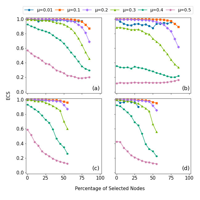
Figure 14: Mean ECS using DeepWalk method over the percentage of selected nodes on LFR benchmark graphs with $1,000$ nodes. (a) and (b) use random node selection while (c) and (d) use targeted node selection.

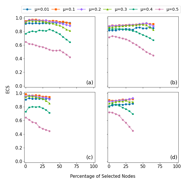
Figure 15: Mean ECS using DeepWalk method over the percentage of selected nodes on LFR benchmark graphs with $10,000$ nodes. (a) and (b) use random node selection while (c) and (d) use targeted node selection.

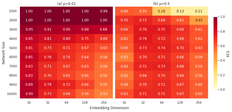
Figure 16: Heatmaps with DeepWalk embedding method. For given embedding dimension and LFR network with given size, the ECS similarity score between ground-truth community structure and detected community structure is recorded.

III.2.2 Large-scale information network embedding (LINE)

The large-scale information network embedding (LINE) method aims to position nodes in close proximity to each other as their similarity increases. LINE can be implemented based on first-order similarity, second-order similarity, or both. According to [14], it works the best when implemented based on first-order similarity, i.e., adjacency of nodes. In fact, for un-weighted network, LINE method based on first-order similarity minimize this objective function:

$$-\sum_{(i,j)\in E}\log\Bigl{(}\frac{1}{1+\exp{(-\mathbf{x}_{i}\cdot\mathbf{x}_{j})}}\Bigr{)},$$

where $E$ is the edge set and $\mathbf{x}_{i}$ denotes the vector indicating the position of the point representing node $i$ in the embedding.

The optimization process of LINE method utilizes stochastic gradient descent, which is enhanced by an edge-sampling treatment, as detailed in [32]. Specifically, the utilization of the LINE embedding method necessitates the presence of GPU for computation. In our study, the machine learning model was trained using a batch size of $8192$ over $100$ epochs, facilitating iterative updates to the embedding vector across the entire training dataset.

Our experimental results, generated through the LINE embedding method, are presented in Figs. 17 and 18. The LINE embedding method produces higher ECS scores when applied to larger networks. Our analysis of networks with 1,000 nodes in Fig. 17 reveals that curves exhibit a steep decline followed by a subsequent increase, but we notice that increasing the embedding dimensions in LINE is expected to mitigate the sharpness of this decline and increase; see Appendix A for details. Owing to the substantial computational demands of the LINE embedding method, we omit the heatmap analysis specifically for LINE.

Based on the aforementioned observation, LINE becomes a viable option for network clustering when dealing with relatively larger networks and the computational resources, particularly GPUs, are available.

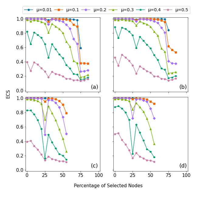
Figure 17: Mean ECS using LINE method over the percentage of selected nodes on LFR benchmark graphs with $1,000$ nodes. (a) and (b) use random node selection while (c) and (d) use targeted node selection.

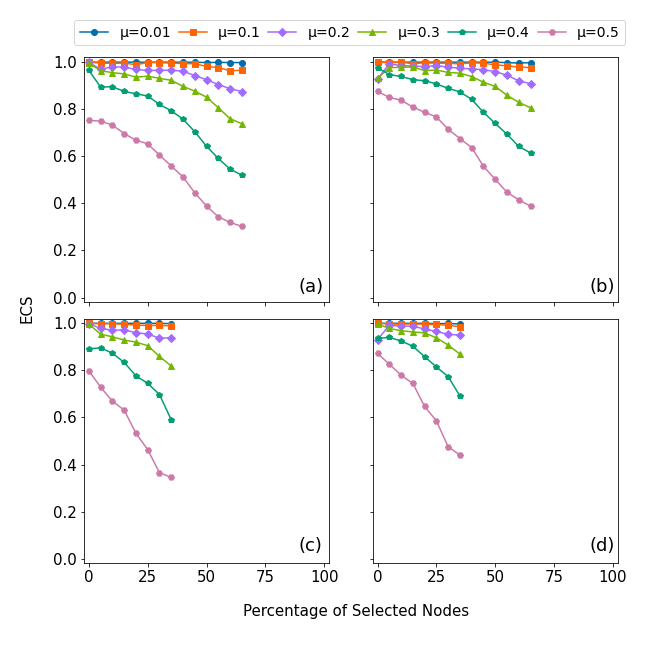
Figure 18: Mean ECS using LINE method over the percentage of selected nodes on LFR benchmark graphs with $10,000$ nodes. (a) and (b) use random node selection while (c) and (d) use targeted node selection.

III.2.3 node2vec

node2vec employs a similar optimization procedure to DeepWalk, but the process of generating “sentences” differs [33]. Specifically, simple random walk is used for DeepWalk, while biased random walk is utilized for node2vec. These biased random walks are composed of a blend of steps following both breadth-first and depth-first search strategies, with parameters $p$ and $q$ controlling the respective influences of these two strategies (see [33] for details about how random walk are generated in node2vec). Therefore, node2vec produces higher-quality and more informative embeddings than DeepWalk. We use the following parameters in our experiments: random walk length $t=40$, window size $w=10$, number of walks per node $n=80$, biased walk weights $p=1$ and $q=1$. Our experimental results on the impact of edge removal, generated through the node2vector embedding method, are reported in Figs. 19 and 20. The heatmaps in Fig. 21 illustrate that node2vec proves to be robust method to produce community detection outcome with high ECS, particularly for strongly clustered networks. In Fig. 21(b) for weakly clustered networks (i.e., $\mu=0.5$), to get high ECS, in general, lower embedding dimensions produce more robust community partition for networks with small sizes; higher embedding dimensions produce more robust community partition for networks with larger sizes.

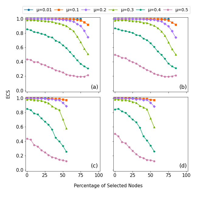
Figure 19: Mean ECS using node2vec method over the percentage of selected nodes on LFR benchmark graphs with $1,000$ nodes. (a) and (b) use random node selection while (c) and (d) use targeted node selection.

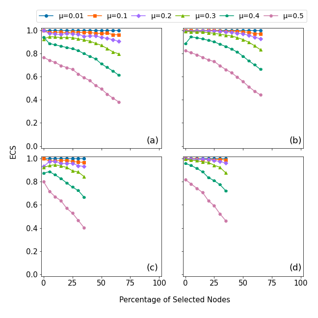
Figure 20: Mean ECS using node2vec method over the percentage of selected nodes on LFR benchmark graphs with $10,000$ nodes. (a) and (b) use random node selection while (c) and (d) use targeted node selection.

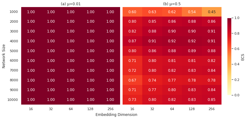
Figure 21: Heatmaps with node2vec embedding method. For given embedding dimension and LFR network with given size, the ECS similarity score between ground-truth community structure and detected community structure is recorded.

We derive the following insights for random walk methods. In the cases of LINE and node2vec, we consistently observe a decrease in ECS as we iteratively select additional nodes and remove their adjacent edges, which aligns with our intuitive expectations. However, DeepWalk exhibits some unexpected increases in ECS. Moreover, for smaller values of the mixing parameter $\mu$, the corresponding curve tends to exhibit higher values. When employing targeted node selection, the ECS experiences a more significant and rapid decline contrasted with random node selection. For example, for LFR network with $1,000$ nodes and $\mu=0.5$, when perturbing the network at $50\%$ and using node2vec with $16$-dimensional embedding, we notice that targeted node selection decreases ECS from $0.43$ to $0.13$ (a decrease of $69.8\%$, see Fig. 19(c)), but ECS decreases from $0.43$ to $0.25$ for random node selection (a decrease of $41.9\%$, see Fig. 19(a)).

When considering the application of random walk embeddings for community detection, node2vec consistently proves to be a more robust choice over DeepWalk and LINE, across networks of varying sizes, the strength of the initial community partition, and perturbation type.

III.3 Comparison of graph embedding methods

In preceding sections, we utilized heatmaps to assess the performance of graph embedding methods for various network sizes and embedding dimensions. To compare community detection outcomes given by various embedding techniques, we conduct cross-comparisons between six data clustering methods. Due to the high computational cost associated with the LINE embedding method, we exclude it from our comparative analysis. The corresponding heatmap for cross-comparison is depicted in Fig. 22. Specifically, Fig. 16(a) comprises a $10\times 5$ matrix, totaling $50$ entries, which we interpret as a $50$-dimensional vector for analysis. Thus, for $\mu=0.01$ or $\mu=0.5$, we obtained a $50$-dimensional vector for each data clustering method based on LE, LLE, HOPE, M-NMF, DeepWalk, and node2vec. These six vectors (given by six data clustering methods) underwent cross-comparison by calculating cosine similarity. In other words, heatmap cells in Fig. 22 reveal the similarity between data clustering results obtained by different methods. Notably, we observe that LE and LLE yield similar data clustering results. However, the results obtained by HOPE were not as closely aligned with those by LE and LLE, although HOPE is also in the family of matrix factorization methods. DeepWalk and node2vec, as two methods in the family of random walk methods, also exhibit similar results. Remarkably, M-NMF yield results significantly divergent from those produced by other methods.

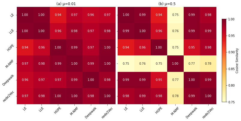
Figure 22: Cross comparison between data clustering methods.

III.4 Results on real-world networks

In this section, we present the results of our experiments conducted on two real-world networks with labeled communities, i.e., the email-EU-core network and the AS network. The email-EU-core network is constructed using email data sourced from a prominent European research institution, comprising $986$ nodes and $16,687$ edges [63]. The AS network, derived from the AS Internet topology data collected in June 2009 by the Archipelago active measurement infrastructure, represents the inter-domain Internet topology with Autonomous Systems (ASes) as nodes and AS peerings as links, forming an AS-level topology graph. This dataset comprises $23,748$ nodes and $58,414$ edges. We select them because they closely resemble power-law degree and community size distributions, as the synthetic networks counterpart (i.e., LFR benchmark graphs). To confirm the alignment of these real-world networks with the properties of LFR networks, we conducted statistical tests using the Python package powerlaw based on the statistical test derived in the work by Clauset et al [66]. The results indicate that both the email-EU-core network and the AS network exhibit power-law characteristics [67]. Specifically, in the email-EU-core network, the degree distribution adheres to a power-law distribution and the community size sequence follows exponential distribution; while in the AS network, both degree and community size distributions conform to power laws.

As discussed in Section II.2, in experiments involving LFR networks, we ensure that the removal of edges from each set of nodes does not result in the disconnection of the remaining network — a prerequisite for graph embedding methods. However, such a stringent requirement is often impractical for real-world networks. For instance, randomly selecting $5\%$ of nodes in the email-EU-core network and deleting their adjacent edges would typically leave the remaining portion of the network disconnected. To address this issue in our experiments with real-world networks, we adopt an alternative approach. In particular, we randomly introduce edges between connected components to restore connectivity. Subsequently, we proceed with the embedding of the reconnected network.

We report experimental results using different embedding methods on these two real-world networks in Figs. 23 and 24. Comparing the two rows of Fig. 23, we can see that when employing targeted node selection, the ECS experiences a more significant decrease than the case of random node selection. For example, for the email-EU-core network, when perturbing it at $50\%$ and using node2vec with $16$-dimensional embedding, we notice that targeted node selection decreases ECS from $0.41$ to $0.31$ (a decrease of $24.3\%$, see Fig. 23(c)), but ECS is only decreased by around $0.02$ by random node selection. Furthermore, LLE and node2vec proved to be the superior choices among all seven embedding methods. In fact, curves corresponding to these two methods in Figs. 23 and 24 are higher in position than other curves.

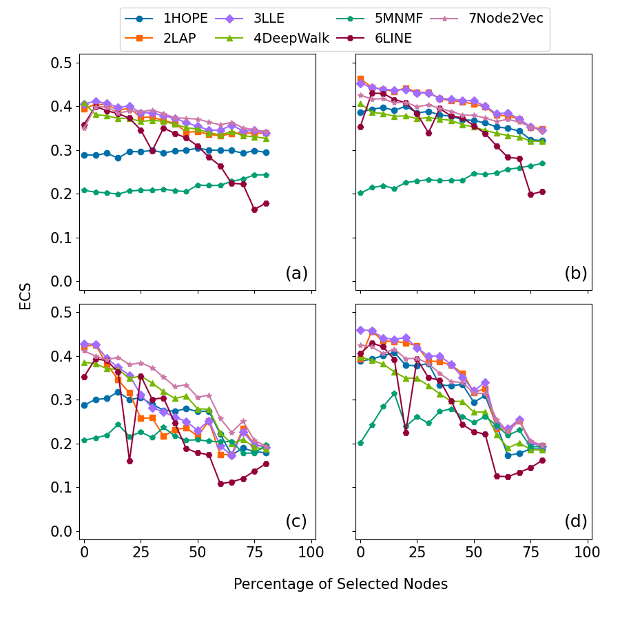
Figure 23: Mean ECS for various methods over the percentage of selected nodes on email-EU-core network (with $986$ nodes). (a) and (b) use random node selection while (c) and (d) use targeted node selection. (a) and (c) corresponds to $16$-dimensional embeddings while (b) and (d) corresponds to $32$-dimensional embeddings.

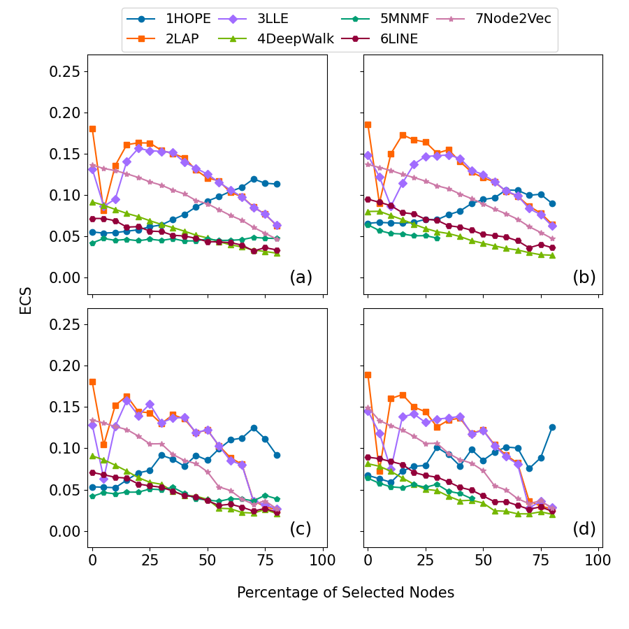
Figure 24: Mean ECS for various methods over the percentage of selected nodes on AS network (with $23,748$ nodes). (a) and (b) use random node selection while (c) and (d) use targeted node selection. (a) and (c) corresponds to $16$-dimensional embeddings while (b) and (d) corresponds to $32$-dimensional embeddings.

IV Conclusion

We conducted a systematic set of experiments aimed at evaluating the robustness of graph embedding methods for community detection on networks. Our study encompassed LFR benchmark graphs and two real-world networks, with variations in network sizes and mixing parameters considered for the LFR benchmark graphs. We studied two different strategies for perturbations: (1) edge removal based on random node selection, analogous to random network errors, and (2) edge removal based on targeted node selection, modeling deliberate attacks. Both perturbation strategies involve the removal of adjacent edges after selecting nodes. Our community detection approach utilized seven graph embedding methods. Community similarity was measured through ECS.

Our experimental findings revealed a general decline in community similarity as more nodes were selected and their adjacent edges deleted. Notably, targeted node selection led to a more pronounced and rapid decline in community similarity compared to random node selection. Analysis of clustering similarity scores suggested that LFR networks with lower mixing parameters, indicative of a stronger community structure, exhibit greater robustness to network perturbation. Moreover, diverse graph embedding methods displayed varying degrees of robustness in network community detection. Specifically, LLE and LE demonstrated proficiency within the family of matrix-based methods. For smaller real-world networks with a limited number of vertices, the more robust embedding method is LLE with a modest embedding dimension, typically on the order of tens — such as the 16 dimensions employed in our experiment. In the case of larger real-world networks, the LE embedding method showed greater robustness to partition. Specifically, a higher embedding dimension is preferable when the community structure is less pronounced, whereas a lower embedding dimension is more effective when the network exhibits a stronger community structure. Within the family of random walk methods, our results consistently highlighted node2vec as the superior choice. Notably, node2vec also outperformed all methods within the family of matrix factorization methods.

In contemplating potential avenues for future research, it is noteworthy that our current experiments did not involve parameter optimization in the graph embedding algorithms, primarily due to its inherent computational expense. To attain a more exhaustive and comprehensive insight into the robustness of community detection using graph embedding methods, we may explore the incorporation of parameter optimization in our forthcoming studies.

Appendix A LINE method with higher embedding dimensions

For the LINE embedding method, our analysis of networks with 1,000 nodes in Fig. 17 reveals a distinct trend: the curves exhibit a steep decline followed by a subsequent increase. According to our experiments, increasing the embedding dimensions in LINE is expected to mitigate the sharpness of this decline and increase, rendering the pattern less pronounced, as indicated in Fig. 25.

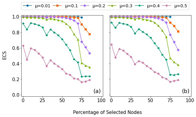
Figure 25: Mean ECS using LINE method over the percentage of selected nodes uniformly at random on LFR benchmark graphs with $1,000$ nodes. The first plot displays results using $128$-dimensional embedding; the second plot displays results using $256$-dimensional embedding.

However, for other embedding methods, a higher embedding dimension doesn’t necessarily lead to better performance with higher ECS scores. For instance, M-NMF with higher dimensions results in lower ECS scores, as shown in Fig. 26, compared to the first row of Fig. 11.

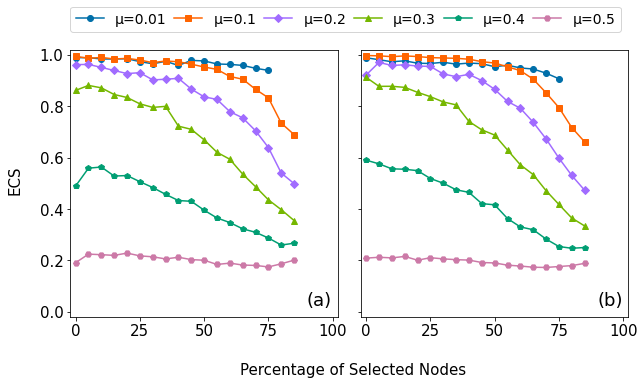
Figure 26: Mean ECS using M-NMF method over the percentage of selected nodes uniformly at random on LFR benchmark graphs with $1,000$ nodes. The first plot displays results using $128$-dimensional embedding; the second plot displays results using $256$-dimensional embedding.