UCB-driven Utility Function Search for Multi-objective Reinforcement Learning
Abstract
In Multi-objective Reinforcement Learning (MORL) agents are tasked with optimising decision-making behaviours that trade-off between multiple, possibly conflicting, objectives. MORL based on decomposition is a family of solution methods that employ a number of utility functions to decompose the multi-objective problem into individual single-objective problems solved simultaneously in order to approximate a Pareto front of policies. We focus on the case of linear utility functions parameterised by weight vectors w. We introduce a method based on Upper Confidence Bound to efficiently search for the most promising weight vectors during different stages of the learning process, with the aim of maximising the hypervolume of the resulting Pareto front. The proposed method is shown to outperform various MORL baselines on Mujoco benchmark problems across different random seeds. The code is online at: https://github.com/SYCAMORE-1/ucb-MOPPO.
123
1 Introduction
A multi-objective sequential decision making problem can be formulated as a multi-objective Markov Decision Process (MOMDP) defined by the tuple with state space , action space , state transition probability , discount factor , initial state distribution , and vector-valued reward function specifying one-step reward for each of the objectives. A decision-making policy maps states into actions, for which a vector-valued value function is defined as:
| (1) |
where is the length of the horizon.
In cases where the objectives conflict with each other, no single optimal policy exists that maximises all objectives simultaneously. The best trade-offs among the objectives are defined in terms of Pareto optimal. A policy is said to dominate if , and it is Pareto optimal if there is no other policy that dominates it. The set of Pareto optimal policies is called the Pareto front. In many real-world applications, an approximation to the Pareto front is required by a decision maker in order to select a preferred policy [14].
A Pareto optimal solution of a multi-objective sequential decision-making problem is an optimal solution of a single-objective problem, given a utility function that aggregates objectives into a scalar reward, mapping the multi-objective value of the policy into a scalar value [10]. Therefore approximation of the Pareto front can be decomposed into a number of scalar reward sub-problems defined by a set of utility functions, bridging methods of Multi-objective Reinforcement Learning (MORL) [14, 12] with methods of multi-objective optimisation based on decomposition [33] collectively referred to as MORL based on Decomposition MORL/D [12].
The space of utility functions for a MORL problem is typically populated by linear and non-linear functions of . In this work we focus on the highly prevalent case where the utility functions are linear, taking the form of , where scalarisation vector w provides the parameterisation of the utility function. Each element of specifies the relative importance (preference) of each objective. The space of linear scalarisation vectors W is the m-dimensional simplex: . For any given w, the original MOMDP is reduced to a single-objective MDP.
Linear utility functions enable MORL to generate a Convex Coverage Set (CCS) of policies, which is a subset of all possible policies such as there exists a policy in the set that is optimal with respect to any linear scalarisation vector w:
| (2) |
CCS is a subset of Pareto front defined for monotonically increasing utility functions [14]. CCS is practically a sufficient solution set for a large class of real-world problems and facilitates more efficient solutions [14]. At the same time, the underlying linear utility function space (space of scalarisation vectors W) is easier to search than that of arbitrarily-composed utility functions, where one has to search for the overall function composition out of primitive function elements (i.e. arithmetic, logarithmic, exponentiation).
MORL/D methods for approximating the CCS can be single-policy or multi-policy [12]. Single-policy methods learn one policy that is conditioned with the parameters of the utility function (scalarisation vector w) [1, 3, 19, 32], while multi-policy approaches maintain a separate policy for each scalarisation vector [21, 31]. Parameter sharing improves the sample efficiency of single-policy methods and allow for generalisation to new objective preferences [1, 32]. Additionally single-policy methods do not require the maintenance of a Pareto archive of policies as in the case of multi-policy methods, significantly reducing computational, memory, and storage requirements.
The way in which scalarisation vectors w are sampled from scalarisation weight simplex W impacts the quality of the CCS serving as an approximation of the Pareto front. Weight vectors can be generated periodically uniform randomly (, and ) [1, 7, 19, 22, 32], or sampled from a set of evenly distributed weight vectors specified a priori [18, 31], or generated by adaptive search methods [3, 21]. In cases where weight vectors are enumerated a priori, a small step-size is required to ensure a good quality CCS is discovered [26].
Our work builds upon good practices of MORL/D and introduces an Upper Confidence Bound (UCB) acquisition function to search for the most promising linear scalarisation vectors to train on at different stages of the learning process, driven by the Pareto front quality metric of hypervolume [11]. We extend the work of [1] by considering a weight-w-conditioned Actor-Critic network instead of a Q-network for . We adopt a multi-policy approach that allows for each policy to specialise into a sub-space of W. Similar to the work of [31] we formulate the problem of maximising the hypervolume of the Pareto front as a surrogate-assisted optimisation problem, in which a data-driven surrogate model predicts the expected change of an objective value resulting from training with weight vector for iterations using Proximal Policy Optimisation (PPO) [27]. The predictions of change of each objective are used to select the weight vectors that are expected to best improve the hypervolume of the Pareto front at each consecutive training stage. At the same time, we extend the work of [31], by leveraging the uncertainty of surrogate model predictions in a UCB acquisition function that balances exploration and exploitation during search. In addition, we extend the work of [31] by using scalarisation-vector-conditioning of instead of maintaining large Pareto archives of policies trained for specific scalarisation vectors.
In summary, two contributions distinguish our work from previous systems of MORL/D:
-
1.
A two-layer problem decomposition allows for different policies to specialise in different sub-spaces of the scalarisation vector space at the first layer, while scalarisation vector conditioning allows for finer decomposition into sub-problems within a sub-space. Policies can benefit from effective generalisation among local neighbouroohds of scalarisation vectors to improve hypervolume and sparsity metrics [11] of the resultant CCS.
-
2.
The use of a UCB acquisition function for selecting from a finite set of evenly distributed scalarisation vectors to balance exploration and exploitation.
The rest of the paper is structured as follows. Prior work on gradient-based and evolutionary MORL is reviewed in Section 2. The proposed method is described in Section 3. Experiments on six multi-objective benchmark problems are outlined in Section 4, and state-of-the-art results on these problems are discussed in Section 5. Finally, we conclude in Section 6 with directions for future research. Supplementary material is provided at https://github.com/SYCAMORE-1/ucb-MOPPO/tree/main/doc.
2 Related Work
A thorough review of MORL can be found in [14]. In this section we highlight previous work that employs either gradient-based or evolutionary learning with a linear utility function.
2.1 Gradient-based MORL
In the case of gradient-based learning, previous MORL work can be classified into three main categories. In the first category, a single policy is trained using a linear scalarisation function for the case where the user’s preferences are known a priori [23, 29].
When user preferences are unknown or difficult to specify, a CCS of policies is computed. In the second category, multiple independent policies are trained using different scalarisation vectors to capture different trade-offs between objectives in order to approximate a CCS. The work of [21] proposes Optimistic Linear Support, a method that adaptively selects the weights of the linear utility function via the concepts of corner weights and estimated improvement to prioritise those corner weights. In [22] a Pareto archive is populated with policies trained with different scalarisation vectors sampled at random in a sequence using vectorised versions of R-learning and H-learning. A method to select a scalarisation vector among the corner weights to more rapidly learn the CCS is presented in [3]. The proposed prioritisation of the weight vectors is based on the magnitude of the improvement that can be formally achieved via generalised policy iteration. A MORL/D method is presented in [17] in which a set of single-objective sub-problems are created based on a set of uniformly spread scalarisation vectors, and a neighbourhood-based parameter transfer strategy is used to solve the sub-problems in sequence by transferring the NN weights. The work of [31] maintains a Pareto archive of policies by focusing on those scalarisation vectors that are expected to improve the hypervolume and sparsity metrics of the resulting Pareto front the most. They formulate the problem of sampling scalarisation vectors as a surrogate-assisted optimisation problem that employs an analytical surrogate model to predict improvements in Pareto front quality as a function of the scalarisation weights.
The third category of methods maintains a single policy that is conditioned on the scalarisation vector w. A number of works train a single policy with the aim of few-shot adaptation to different objective preferences [1, 7, 32]. The work of [1] considers a scalarisation-vector-conditioned Q-network that is trained to solve the corresponding single-objective RL sub-problem for w sampled at random (, and ). The Q-network is tasked to generalise across changes in w reflecting changes in the relative preference among objectives. Similar to [1], the work of [32] uses Envelope Q-learning to train a single Q-network conditioned on scalarisation vectors sampled uniform randomly with the aim of few-shot adaptation to new scalarisation vectors on demand. In a similar vein the work of [7] trains a PPO-based meta-policy that is tasked to generalise across a number of scalarisation vectors. The meta-policy is trained collaboratively using data generated from policies specialised to scalarisation vectors sampled uniform randomly. The Pareto front is then created by few-shot fine-tuning of the meta-policy with different scalarisation vectors.
Directly approximating the CCS using a single policy conditioned on a scalarisation vector has been studied in [18, 19]. The work of [19] adds a concave term (the entropy of the policy) to the regular reward of Soft Actor Critic to train the policy and the Q-network that are both conditioned on the scalarisation vector sampled uniform randomly, while the work of [18] extends the work of [31] with scalarisation-vector-conditioning that allows to maintain a single policy instead of a Pareto archive of multiple policies.
2.2 Evolutionary MORL
The orthogonal strengths and weaknesses of Evolutionary Algorithms [8] and gradient-based MORL motivate hybrid algorithms [4]. Representative works [6, 20, 28] have demonstrated that combining both approaches yields high quality Pareto fronts, quantified by metrics such as hypervolume and sparsity.
A two-stage hybrid algorithm for MORL is proposed in [6]. In the pretraining stage, multiple policies with shared layers are trained using Soft Actor-Critic with separate scalarisation vectors. In the fine-tuning stage, a multi-objective Evolution Strategy further optimises the weights of the policies, while certain shared layers are kept frozen. This approach aims at discovering policies that reside in concave regions of the Pareto front.
A population-based algorithm for MORL, named EMOGI, is introduced in [28]. An evolutionary algorithm searches the space of scalarisation vectors W and associated policy parameters, and the Asynchronous Advantage Actor-Critic algorithm is used to further fine-tune the population of policies using the corresponding scalarised reward functions. Non-dominated sorting is applied to maintain a set of Pareto optimal policies.
The work of [20] employs a surrogate-assisted multi-objective evolutionary algorithm to approximate a CCS of policies. A set of scalarisation vectors uniformly distributed in space W are used to train policies using a Policy Gradient algorithm. Data from trained policies are used to build computationally inexpensive surrogate models that predict the average return and the standard deviation of the return as a function of a policy’s parameters (weights of NN). Control is then passed to a surrogate-assisted Neuro-evolution algorithm that uses probabilistic selection method based on surrogate model’s predictions and the corresponding estimates of prediction uncertainty. Multi-objective Policy Gradient training is interleaved with surrogate-assisted Neuro-evolution for a number of iterations.
3 Methods
MORL/D is adopted as the solution framework. The key technical characteristics of the proposed algorithm, named UCB-MOPPO, are as follows:
- Decomposition of MORL problem into scalar RL sub-problems.
-
The overall scalarisation weight simplex W is decomposed into sub-spaces as shown in Figure 2(a). A separate policy is trained for each sub-problem by conditioning it on scalarisation vectors sampled from the associated sub-space .
- Scalarisation-vector-conditioned Actor-Critic.
-
Given a policy network , a value network and a scalarisation vector w , the MO Actor-critic algorithm aims to maximise the weighted-sum of expected rewards . Following the works of [1, 19, 32] both the policy network and the value network are conditioned on scalarisation vector w. This allows for a single policy to express different trade-offs between objectives by generalising to a neighbourhood of scalarisation vectors.
- Surrogate-assisted maximisation of CCS hypervolume.
-
An acquisition function based on Upper Confidence Bound [30] is used to select those scalarisation vectors to train on from each sub-space . At each stage of the training process the selected scalarisation vectors are those expected to maximise the hypervolume of the resulting CCS the most.
The pseudo-code of UCB-MOPPO is given in supplementary material, Section 1, Algorithm 3.
3.1 Two-layer decomposition of MORL problem into scalar RL sub-problems
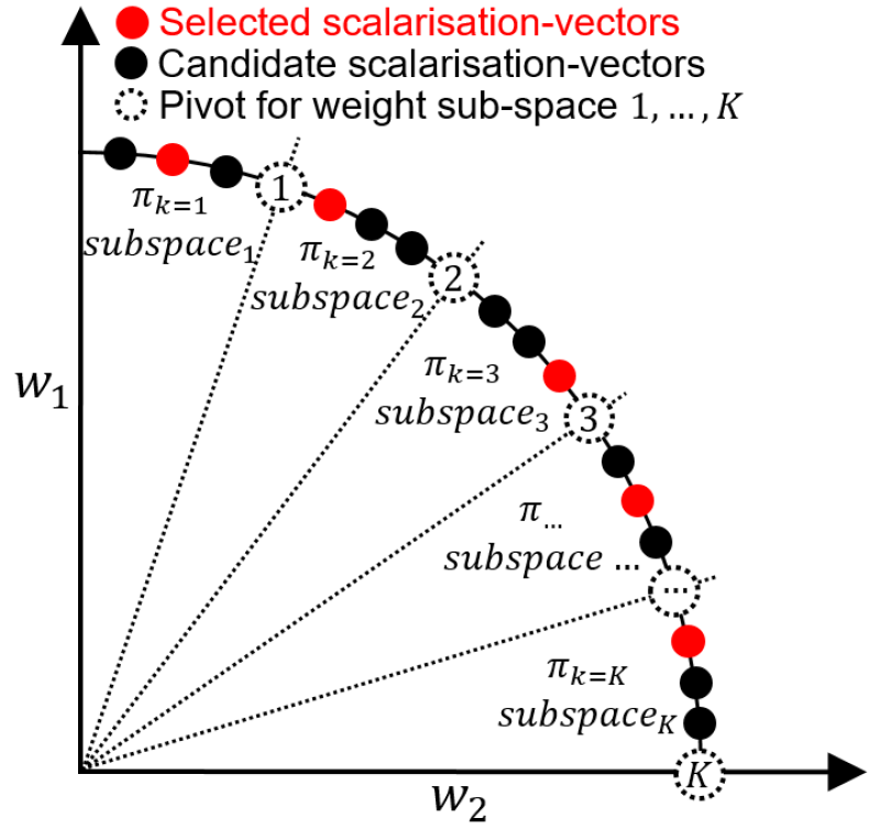
At the first layer of problem decomposition, a set of evenly distributed scalarisation vectors, named as pivots, are defined within the scalarisation vector space W. These pivot vectors effectively divide W into different sub-spaces as shown in Figure 2(a). The system allows to independently train multiple pivot policies with different random seeds in order to improve the density of the resulting CCS. At the second layer of problem decomposition, for each sub-space , , a number of evenly distributed scalarisation vectors are defined in turn. Therefore the overall MORL problem is decomposed into a total of scalar RL sub-problems, defined as follows for a fixed w:
| (3) |
A separate policy (pivot policy) is independently trained for each sub-space by conditioning on the corresponding scalarisation vectors. As an example, for a bi-objective problem with in Figure 2(a), for two sub-spaces , with , , . The solutions of the sub-problems compose a CCS.
3.2 Scalarisation-vector-conditioned Actor-Critic
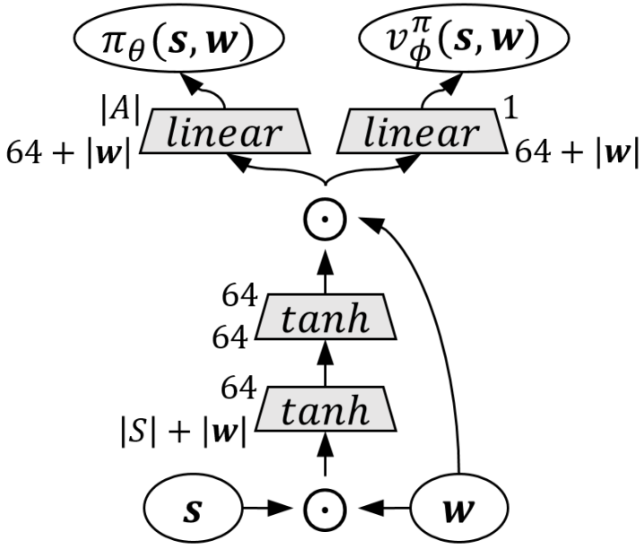
The NN architecture of the Actor-Critic is illustrated in Figure 1. The state vector s concatenated with the scalarisation vector w form the input layer. w is also concatenated with the last shared layer through a residual connection [15]. Residual connections aim at improving the sensitivity of NN output to changes in w in a similar vein with reward-conditioned policies in [16].
3.3 Surrogate-assisted maximisation of CCS hypervolume
3.3.1 Overview
The learning algorithm proceeds in stages of iterations each. At every stage, pivot policies , are trained in parallel using PPO, each conditioned on a subset of scalarisation vectors out of in total that are defined for each corresponding sub-space , , with . The selection of scalarisation vectors to train on at each stage is performed via surrogate-assisted maximisation of the hypervolume of the CCS. First, a data-driven uncertainty-aware surrogate model is built in the scalarisation vector space to predict the expected change in each objective after training conditioned on said scalarisation vectors for iterations. Second, an acquisition function is defined as the Upper Confidence Bound (UCB) of the CCS hypervolume that is expected by including a scalarisation vector to the policy’s conditioning set at each training stage. Maximising the acquisition function selects the scalarisation vectors that are expected to improve CCS hypervolume the most. Pseudo code can is provided in supplementary material, Section 1, Algorithm 3.
3.3.2 Warm-up phase
The algorithm starts with a warm-up stage performed using Algorithm 1. For an -objective problem, a set of evenly distributed pivot vectors are generated, and a set of pivot policies, each conditioned on a separate pivot vector, is trained for a number of epochs.
3.3.3 Surrogate model
Let be the policy that results from the policy during the training stage of iterations. Let be the change in the value of the objective for the policy conditioned on scalarisation vector w trained with PPO for iterations. For each pivot policy , , and for each objective , a separate dataset is created using policy’s evaluation data of objective that are collected from the simulation environment during a number of consecutive training stages , as follows:
| (4) |
A surrogate model is trained on to predict as a function of the scalarisation vector w, for number of objectives. The training is incremental while additional tuples are appended to from consecutive training stages. The surrogate model takes the form of Bagging [5] of linear models with elastic net regularisation [34]. Bagging trains independently linear models on bootstrap samples of the original training data and predicts using their average, that is . An estimate of the epistemic uncertainty of the prediction can be computed using the variance of the component model predictions [13], that is .
3.3.4 UCB acquisition function maximisation
For each policy and each objective a surrogate model can predict the expected objective values by conditioning a policy on scalarisation vector w during a training stage as follows:
| (5) |
with a corresponding vectorised prediction over objectives and the accompanying vectorised uncertainty estimate .
At the beginning of each training stage the algorithm needs to select those scalarisation vectors out evenly distributed vectors in each sub-space , that are predicted via the surrogate model to improve the hypervolume of the resulting CCS the most. is a function that computes hypervolume as in [11]. The scalarisation vectors are selected one at a time without replacement in a sequence of invocations of a process that maximises a UCB acquisition function defined on as:
| (6) | ||||
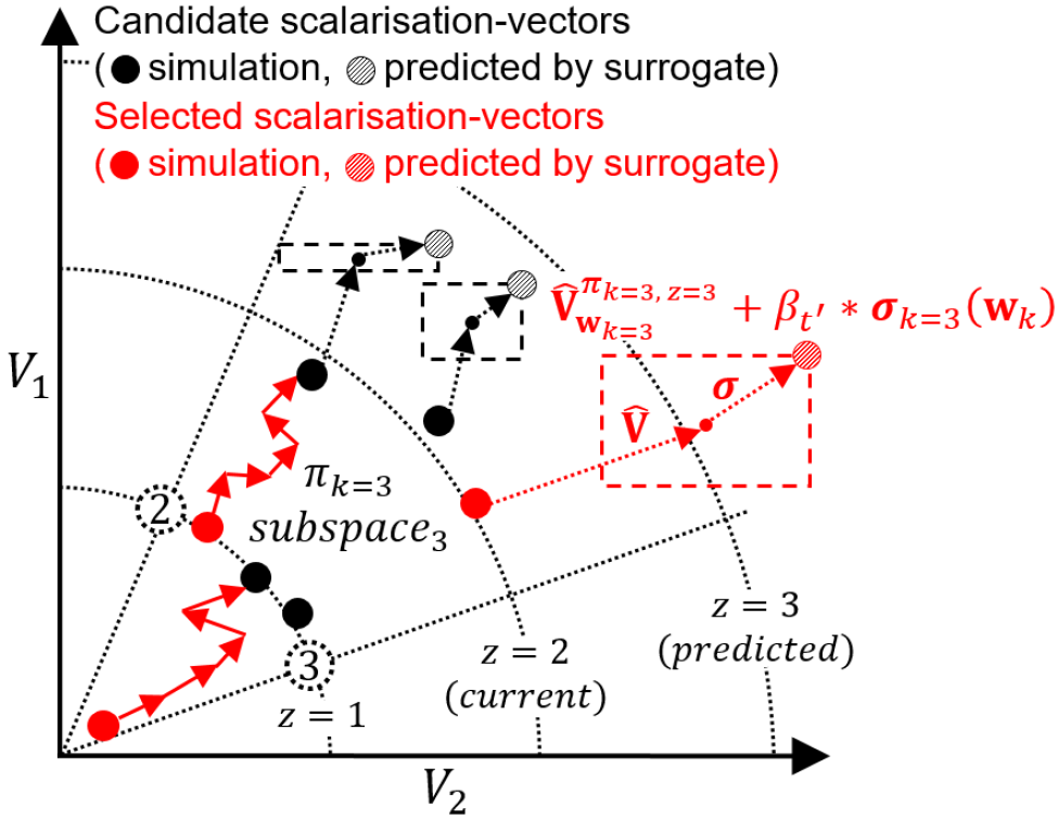
where is a function computing the CCS from a set of objective vectors, and . This UCB formulation assumes maximisation of objectives. Once selected, a scalarisation vector is removed from the candidate set for the current training stage. The process of selecting scalarisation vectors that are expected to maximise the hypervolume of the resulting CCS is illustrated pictorially in Figure 2(b).
3.4 Baseline MOPPO Methods
Three baseline MOPPO methods are implemented to determine the benefits brought by UCB-driven search of the space of scalarisation vectors. In contrast to UCB-MOPPO, the baselines do not explicitly trade-off exploration and exploitation.
-
Random-MOPPO. Similar to Fixed-MOPPO, policies are trained, with one policy for each pivot . During training, policy is conditioned on multiple scalarisation vectors sampled uniform randomly from sub-space . Scalarisation vectors are re-sampled after every timesteps to ensure policies are exposed to a diverse set of scalarisation vectors during training. Pseudocode is provided in Algorithm 2.
-
Mean-MOPPO. This baseline is identical to UCB-MOPPO, except the acquisition function does not take uncertainty into account. Specifically, in the acquisition function defined by Equation 6.
-
PGMORL. This is the system proposed in [31]. It is included as a baseline since it is the first work to introduce a surrogate-assisted optimisation of Pareto front hypervolume, reporting competitive results in Mujoco benchmarks.
4 Experiments
Experiments were carried out on six MORL benchmark problems drawn from the MuJoCo test suite [2], and each problem was ran with 3 different random seeds: Swimmer-V2 (2), Halfcheetah-V2 (2), Walker2d-V2 (2), Ant-V2 (2), Hopper-V2 (2), and Hopper-V3 (3), where the number of objectives is indicated in parentheses. The same problems were considered in [31] to evaluate PGMORL, enabling a straightforward comparison with the proposed UCB-MOPPO algorithm. Detailed descriptions of the objectives, and state and action spaces are provided in the supplementary material, Section 2.
| Parameter | UCB | Mean | Random | Fixed |
| (pivot vectors) | 10 | 10 | 10 | 10 |
| (selected within sub-space) | 10 | 10 | 10 | 1 |
| (sub-space vectors) | 100 | 100 | 10 | 10 |
| Discretisation step-size (layer 1) | 0.1 | 0.1 | 0.1 | 0.1 |
| Discretisation step-size (layer 2) | 0.01 | 0.01 | 0.1 | 0.1 |
| Parameter | UCB | Mean | Random | Fixed |
| (pivot vectors) | 36 | 36 | 36 | 36 |
| (selected within sub-space) | 10 | 10 | 10 | 1 |
| (sub-space vectors) | 117 | 117 | 36 | 36 |
| Discretisation step-size (layer 1) | 0.1 | 0.1 | 0.1 | 0.1 |
| Discretisation step-size (layer 2) | 0.05 | 0.05 | 0.1 | 0.1 |
5 Results Analysis
We evaluate the performance of our proposed method including four baseline methods on six multi-objective RL problems. Hyperparameters for policy neural network initialisation and PPO are aligned with the values recommended in Stable-Baselines3 [24], hyperparameters are provided in Section 3 of the supplementary material. Each algoritmh is
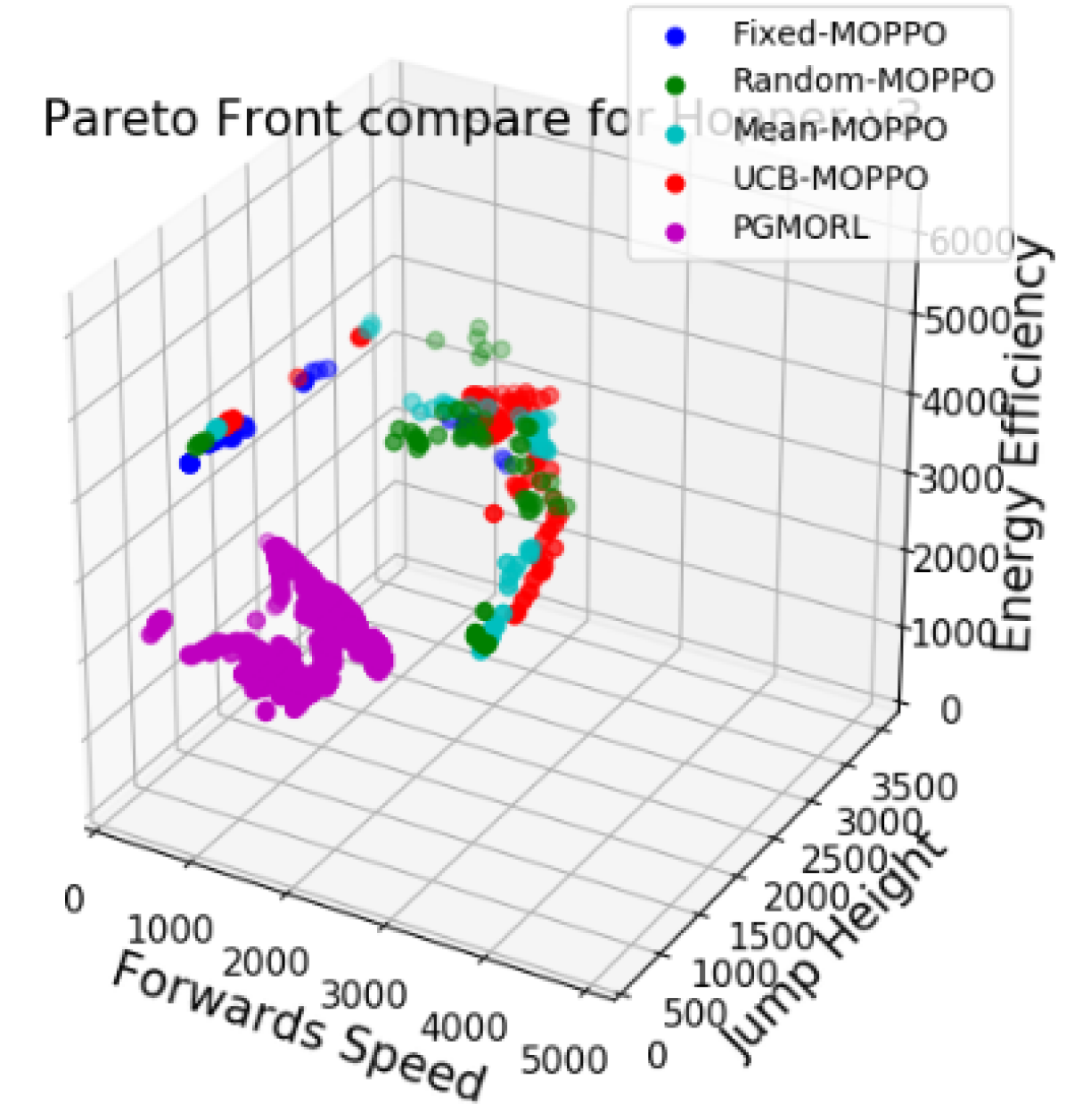
5.1 Quality of the Pareto Fronts
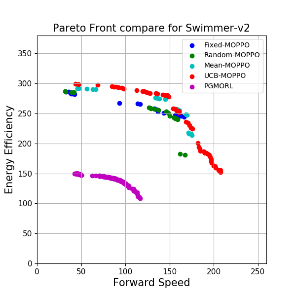
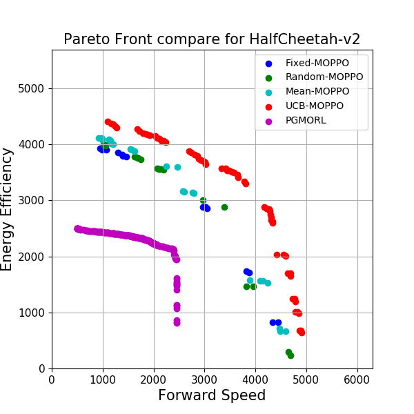
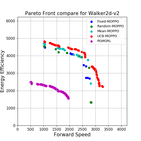
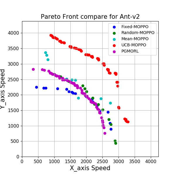
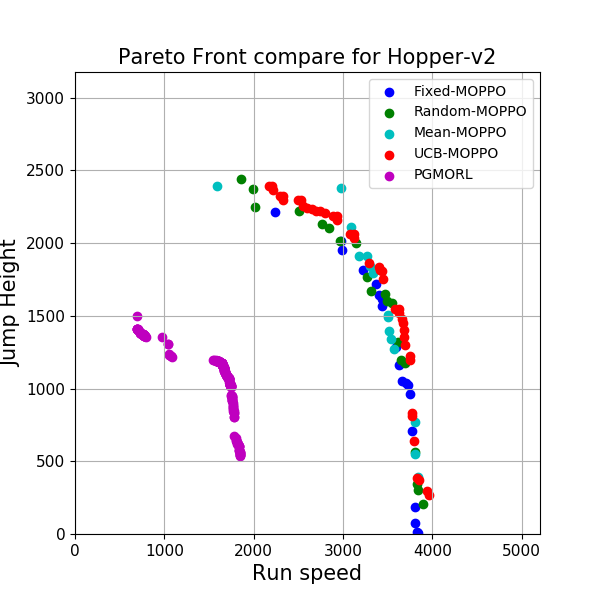
Hypervolumes achieved by UCB-MOPPO and all baseline methods are reported in Table 3, and the Pareto fronts are visualised in Figure 3. UCB-MOPPO achieves significantly higher hypervolume than PGMORL in all six problems. Furthermore, UCB-MOPPO outperforms all MOPPO baselines in all but one problem (Hopper-V2, where Mean-MOPPO is slightly better). This result confirms that selecting scalarisation vectors based on the UCB effectively balances exploration and exploitation during policy learning.
| Benchmark Problem | Hypervolume | UCB-MOPPO (proposed) | Mean-MOPPO | Random-MOPPO | Fixed-MOPPO | PGMORL |
|---|---|---|---|---|---|---|
| Swimmer-V2 | 5.29 | 4.72 | 4.56 | 4.45 | 1.67 | |
| Halfcheetah-V2 | 1.65 | 1.60 | 1.21 | 1.12 | 0.58 | |
| Walker2d-V2 | 1.32 | 1.29 | 1.15 | 1.13 | 0.44 | |
| Ant-V2 | 1.20 | 0.92 | 0.65 | 0.60 | 0.61 | |
| Hopper-V2 | 8.07 | 8.27 | 7.98 | 7.64 | 0.24 | |
| Hopper-V3 | 3.41 | 2.83 | 2.90 | 2.64 | 0.63 |
PGMORL produces dense Pareto fronts because a large number of policies are accumulated in the policy archive. Despite giving rise to dense fronts, PGMORL realises much lower hypervolumes compared to the MOPPO baselines. We attribute the improved hypervolumes in MOPPO to the incorporation of PPO (which brings enhanced stability compared to vanilla policy gradients), and enhanced learning efficiency brought by a two-layer decomposition of the MORL problem.
Fixed-MOPPO is the most lightweight method among the baselines since policies are conditioned on a single fixed scalarisation vector. However, the method renders noticeably lower quality Pareto fronts, as can be seen in Figure 4. This observation underscores the need to condition policies using a diverse set of scalarisation vectors at train time. Despite its relatively low performance, Fixed-MOPPO can be invoked to quickly gain insights into a new MORL problem, for instance to determine if objectives are conflicting.
Random-MOPPO achieves a higher hypervolume and a denser Pareto front compared to Fixed-MOPPO. Random selection of scalarisation vectors during training enables policies to distinguish between different scalarisation vectors with greater fidelity at test time. However, random selection of scalarisation vectors is inefficient, since promising regions of the space are under-explored.
Mean-MOPPO is most competitive method among all the baselines. Indeed, this method attains a larger hypervolume than UCB-MOPPO in Hopper-V2. Mean-MOPPO directs the search towards promising regions, but it tends to produce less dense Pareto fronts than the proposed method leveraging UCB-driven search. Lower quality Pareto fronts can be attributed to the greedy selection of scalarisation vectors based on the mean predicted hypervolume improvement given by the surrogates, without considering the prediction uncertainty.
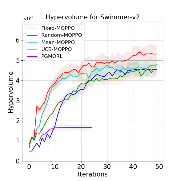
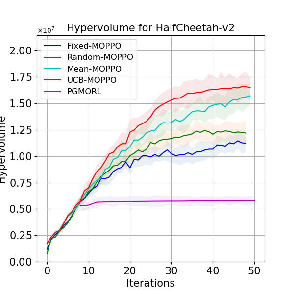
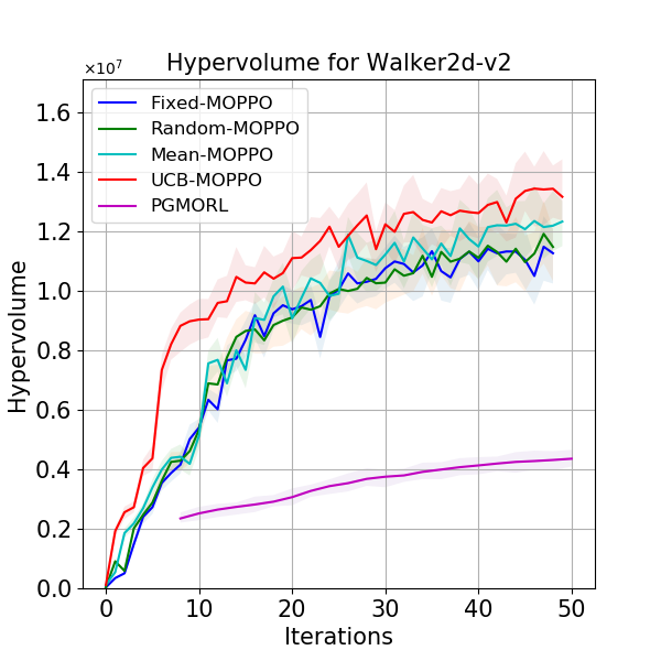

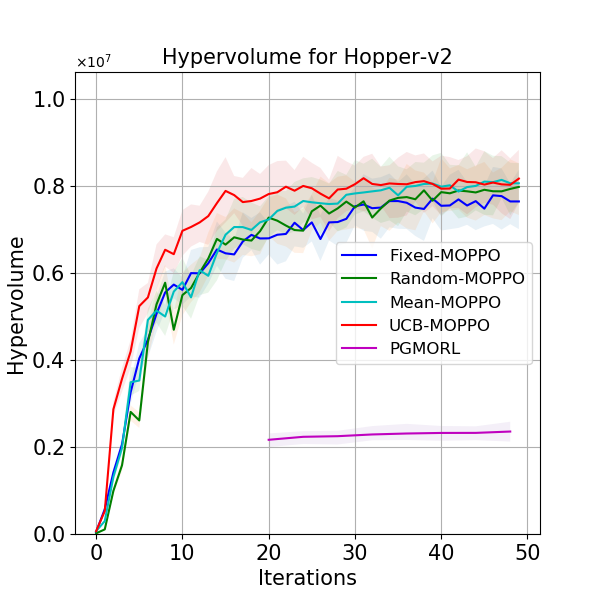
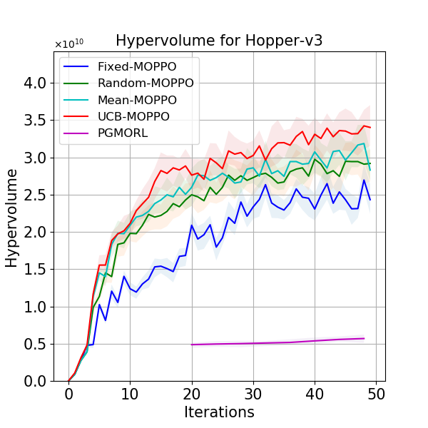
5.2 Convergence speed
As illustrated in Figure 4, UCB-MOPPO (red lines) showcases superior convergence characteristics across the MORL problems. More rapid progress during the early stages of learning is evident in all problems – the proposed method quickly identifies and exploits scalarisation vectors yielding the most significant improvements in hypervolume. This indicates an adept balancing between exploration and exploitation, which is crucial in stochastic MORL problems where objectives are conflicting.
Some baseline methods plateau early, with this being especially pronounced in the case of Ant-V2. This suggests that the myopic baselines are becoming trapped in suboptimal regions of the search space. In contrast, UCB-MOPPO consistently converges more quickly to higher hypervolumes, while sustaining optimisation progress for longer. The superior learning dynamics are primarily attributable to the UCB-driven search mechanism, which efficiently discriminates between known near-optimal scalarisation vectors and more uncertain but high-potential candidates.
5.3 Growth of the Policy Archive in PGMORL
UCB-MOPPO consistently requires fewer policies to construct a satisfactory Pareto front compared to the PGMORL baseline across all tested environments. As depicted in Figure 5, the policy archive size in PGMORL tends to increase linearly, since any policies that improve the Pareto front are subsumed into the archive.
| Methods | Swimmer-v2 | Halfcheetah-V2 | Walker2d-V2 | Ant-V2 | Hopper-V2 | Hopper-V3 |
|---|---|---|---|---|---|---|
| PGMORL | 68 | 285 | 412 | 64 | 206 | 4023 |
| UCB-MOPPO | 30 | 30 | 30 | 30 | 30 | 108 |
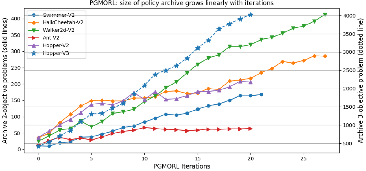
The total number of policies after convergence is displayed in Table 4 for PGMORL and UCB-MOPPO. Some challenging problems result in a large number of policies in the PGMORL archive (e.g. Walker2d-V2 and Hopper-V3). One advantage of all the MOPPO methods is that a small set of policies is maintained and the number of policies does not grow. Therefore, an efficient search in UCB-MOPPO is complemented by a memory-efficient implementation, which can be an important consideration in production environments with tight resource constraints.
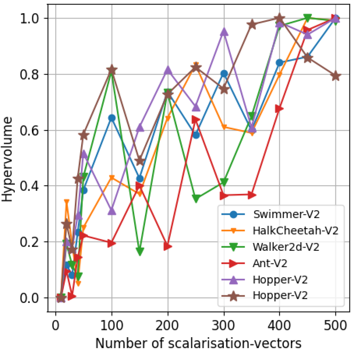
5.4 Interpolating in the space of scalarisation vectors
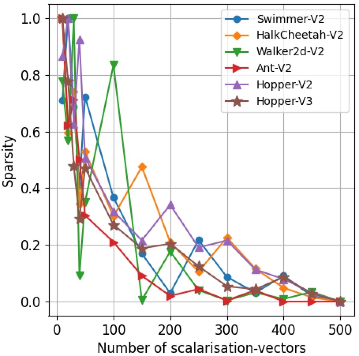
An analysis was carried out to assess the ability of policies trained via UCB-MOPPO to interpolate in a more fine-grained discretisation of vector space , discretised using smaller step-sizes than those considered during training.
Each of the policies, corresponding to the sub-spaces is evaluated on scalarisation vectors. We present the curve of hypervolume and sparsity in Figure 6. The plots illustrate a general trend for hypervolume to improve (increase) with , while sparsity also improves (decreases). Thus, increasing the granularity of the scalarisation vectors improves Pareto front quality, without the need for additional training – a benefit not enjoyed by PGMORL or other approaches for MORL/D.
6 Conclusion
The preferences of a decision maker over conflicting objectives can be represented with a utility function that transforms the MORL problem into a single-objective RL problem. In cases where user preferences are uncertain or undefined, the system is required to produce a set of Pareto optimal solutions that the user can leverage to make informed decisions. MORL/D is a MORL framework that employs a number of utility functions to decompose the MORL problem into several single-objective sub-problems that are solved simultaneously to produce a Pareto optimal set of policies. We focused on the case where the utility functions are linear, parameterised with scalarisation vectors w.
The space of linear scalarisation vectors is very large to systematically enumerate, therefore in this paper we introduced a method to search for those scalarisation vectors that are expected to maximise the quality of the resulting CCS. The salient conclusions of this work are as follows. First, the proposed method was empirically shown to outperform various competitive baselines in terms of CCS hypervolume. Second, the footprint in terms of policies required to be maintained is substantially lower compared to a baseline found in prior work, making the method particularly applicable in computational-resource-constrained environments. Third, we observed that for the proposed method the hypervolume and sparsity metrics of the CCS are a function of the step-size of the discretisation of the scalarisation vector space, with both metrics improving as the step-size becomes smaller. This suggested an effective generalisation ability across local neighbourhoods of scalarisation vectors that is specific to NN architectures based on scalarisation vector conditioning.
References
- Abels et al. [2019] A. Abels, D. M. Roijers, T. Lenaerts, A. Nowé, and D. Steckelmacher. Dynamic weights in multi-objective deep reinforcement learning. In K. Chaudhuri and R. Salakhutdinov, editors, Proceedings of the 36th International Conference on Machine Learning, ICML 2019, 9-15 June 2019, Long Beach, California, USA, volume 97 of Proceedings of Machine Learning Research, pages 11–20. PMLR, 2019. URL http://proceedings.mlr.press/v97/abels19a.html.
- Alegre et al. [2022] L. N. Alegre, F. Felten, E.-G. Talbi, G. Danoy, A. Nowé, A. L. Bazzan, and B. C. da Silva. Mo-gym: A library of multi-objective reinforcement learning environments. In Proceedings of the 34th Benelux Conference on Artificial Intelligence BNAIC/Benelearn, 2022.
- Alegre et al. [2023] L. N. Alegre, A. L. C. Bazzan, D. M. Roijers, A. Nowé, and B. C. da Silva. Sample-efficient multi-objective learning via generalized policy improvement prioritization. In N. Agmon, B. An, A. Ricci, and W. Yeoh, editors, Proceedings of the 2023 International Conference on Autonomous Agents and Multiagent Systems, AAMAS 2023, London, United Kingdom, 29 May 2023 - 2 June 2023, pages 2003–2012. ACM, 2023. 10.5555/3545946.3598872. URL https://dl.acm.org/doi/10.5555/3545946.3598872.
- Bai et al. [2023] H. Bai, R. Cheng, and Y. Jin. Evolutionary Reinforcement Learning: A Survey. Intelligent Computing, 2:0025, 2023.
- Breiman [1996] L. Breiman. Bagging predictors. Mach. Learn., 24(2):123–140, 1996. 10.1007/BF00058655. URL https://doi.org/10.1007/BF00058655.
- Chen et al. [2020] D. Chen, Y. Wang, and W. Gao. Combining a gradient-based method and an evolution strategy for multi-objective reinforcement learning. Applied Intelligence, 50(10):3301–3317, 2020.
- Chen et al. [2019] X. Chen, A. Ghadirzadeh, M. Björkman, and P. Jensfelt. Meta-learning for multi-objective reinforcement learning. In 2019 IEEE/RSJ International Conference on Intelligent Robots and Systems (IROS), pages 977–983, 2019. 10.1109/IROS40897.2019.8968092.
- Eiben and Smith [2015] A. E. Eiben and J. E. Smith. Introduction to Evolutionary Computing, Second Edition. Natural Computing Series. Springer, 2015. ISBN 978-3-662-44873-1. 10.1007/978-3-662-44874-8. URL https://doi.org/10.1007/978-3-662-44874-8.
- Falcón-Cardona and Coello [2021] J. G. Falcón-Cardona and C. A. C. Coello. Indicator-based multi-objective evolutionary algorithms: A comprehensive survey. ACM Comput. Surv., 53(2):29:1–29:35, 2021. 10.1145/3376916. URL https://doi.org/10.1145/3376916.
- Feinberg and Shwartz [1995] E. A. Feinberg and A. Shwartz. Constrained markov decision models with weighted discounted rewards. Math. Oper. Res., 20(2):302–320, 1995. 10.1287/MOOR.20.2.302. URL https://doi.org/10.1287/moor.20.2.302.
- Felten et al. [2023] F. Felten, L. N. Alegre, A. Nowé, A. L. C. Bazzan, E. Talbi, G. Danoy, and B. C. da Silva. A toolkit for reliable benchmarking and research in multi-objective reinforcement learning. In A. Oh, T. Naumann, A. Globerson, K. Saenko, M. Hardt, and S. Levine, editors, Annual Conference on Neural Information Processing Systems 2023, NeurIPS 2023, New Orleans, LA, USA, December 10 - 16, 2023, 2023. URL http://papers.nips.cc/paper_files/paper/2023/hash/4aa8891583f07ae200ba07843954caeb-Abstract-Datasets_and_Benchmarks.html.
- Felten et al. [2024] F. Felten, E. Talbi, and G. Danoy. Multi-objective reinforcement learning based on decomposition: A taxonomy and framework. J. Artif. Intell. Res., 79:679–723, 2024. 10.1613/JAIR.1.15702. URL https://doi.org/10.1613/jair.1.15702.
- Gawlikowski et al. [2023] J. Gawlikowski, C. R. N. Tassi, M. Ali, J. Lee, M. Humt, J. Feng, A. M. Kruspe, R. Triebel, P. Jung, R. Roscher, M. Shahzad, W. Yang, R. Bamler, and X. Zhu. A survey of uncertainty in deep neural networks. Artif. Intell. Rev., 56(S1):1513–1589, 2023. 10.1007/S10462-023-10562-9. URL https://doi.org/10.1007/s10462-023-10562-9.
- Hayes et al. [2022] C. F. Hayes, R. Radulescu, E. Bargiacchi, J. Källström, M. Macfarlane, M. Reymond, T. Verstraeten, L. M. Zintgraf, R. Dazeley, F. Heintz, E. Howley, A. A. Irissappane, P. Mannion, A. Nowé, G. de Oliveira Ramos, M. Restelli, P. Vamplew, and D. M. Roijers. A practical guide to multi-objective reinforcement learning and planning. Auton. Agents Multi Agent Syst., 36(1):26, 2022.
- He et al. [2016] K. He, X. Zhang, S. Ren, and J. Sun. Deep residual learning for image recognition. In Proceedings of the IEEE conference on computer vision and pattern recognition, pages 770–778, 2016.
- Kumar et al. [2019] A. Kumar, X. B. Peng, and S. Levine. Reward-conditioned policies. CoRR, abs/1912.13465, 2019. URL http://arxiv.org/abs/1912.13465.
- Li et al. [2021] K. Li, T. Zhang, and R. Wang. Deep reinforcement learning for multiobjective optimization. IEEE Trans. Cybern., 51(6):3103–3114, 2021. 10.1109/TCYB.2020.2977661. URL https://doi.org/10.1109/TCYB.2020.2977661.
- Liu and Qian [2021] F. Liu and C. Qian. Prediction guided meta-learning for multi-objective reinforcement learning. In IEEE Congress on Evolutionary Computation, CEC 2021, Kraków, Poland, June 28 - July 1, 2021, pages 2171–2178. IEEE, 2021. 10.1109/CEC45853.2021.9504972. URL https://doi.org/10.1109/CEC45853.2021.9504972.
- Lu et al. [2023] H. Lu, D. Herman, and Y. Yu. Multi-objective reinforcement learning: Convexity, stationarity and pareto optimality. In The Eleventh International Conference on Learning Representations, ICLR 2023, Kigali, Rwanda, May 1-5, 2023. OpenReview.net, 2023. URL https://openreview.net/pdf?id=TjEzIsyEsQ6.
- Mazumdar and Kyrki [2024] A. Mazumdar and V. Kyrki. Hybrid Surrogate Assisted Evolutionary Multiobjective Reinforcement Learning for Continuous Robot Control. In International Conference on the Applications of Evolutionary Computation (Part of EvoStar), pages 61–75. Springer, 2024.
- Mossalam et al. [2016] H. Mossalam, Y. M. Assael, D. M. Roijers, and S. Whiteson. Multi-objective deep reinforcement learning, 2016.
- Natarajan and Tadepalli [2005] S. Natarajan and P. Tadepalli. Dynamic preferences in multi-criteria reinforcement learning. In L. D. Raedt and S. Wrobel, editors, ICML, Bonn, Germany, August 7-11, 2005, volume 119 of ACM International Conference Proceeding Series, pages 601–608, 2005. 10.1145/1102351.1102427. URL https://doi.org/10.1145/1102351.1102427.
- Pan et al. [2020] A. Pan, W. Xu, L. Wang, and H. Ren. Additional planning with multiple objectives for reinforcement learning. Knowl. Based Syst., 193:105392, 2020. 10.1016/J.KNOSYS.2019.105392. URL https://doi.org/10.1016/j.knosys.2019.105392.
- Raffin et al. [2021] A. Raffin, A. Hill, A. Gleave, A. Kanervisto, M. Ernestus, and N. Dormann. Stable-baselines3: Reliable reinforcement learning implementations. Journal of Machine Learning Research, 22(268):1–8, 2021.
- Reymond et al. [2023] M. Reymond, C. F. Hayes, D. Steckelmacher, D. M. Roijers, and A. Nowé. Actor-critic multi-objective reinforcement learning for non-linear utility functions. Auton. Agents Multi Agent Syst., 37(2):23, 2023. 10.1007/S10458-023-09604-X. URL https://doi.org/10.1007/s10458-023-09604-x.
- Roijers et al. [2015] D. M. Roijers, S. Whiteson, and F. A. Oliehoek. Point-based planning for multi-objective pomdps. In Q. Yang and M. J. Wooldridge, editors, Proceedings of the Twenty-Fourth International Joint Conference on Artificial Intelligence, IJCAI 2015, Buenos Aires, Argentina, July 25-31, 2015, pages 1666–1672. AAAI Press, 2015. URL http://ijcai.org/Abstract/15/238.
- Schulman et al. [2017] J. Schulman, F. Wolski, P. Dhariwal, A. Radford, and O. Klimov. Proximal policy optimization algorithms. arXiv preprint arXiv:1707.06347, 2017.
- Shen et al. [2020] R. Shen, Y. Zheng, J. Hao, Z. Meng, Y. Chen, C. Fan, and Y. Liu. Generating Behavior-Diverse Game AIs with Evolutionary Multi-objective Deep Reinforcement Learning. In IJCAI, pages 3371–3377, 2020.
- Siddique et al. [2020] U. Siddique, P. Weng, and M. Zimmer. Learning fair policies in multi-objective (deep) reinforcement learning with average and discounted rewards. In Proceedings of the 37th International Conference on Machine Learning, volume 119 of Proceedings of Machine Learning Research, pages 8905–8915. PMLR, 2020. URL http://proceedings.mlr.press/v119/siddique20a.html.
- Srinivas et al. [2010] N. Srinivas, A. Krause, S. M. Kakade, and M. W. Seeger. Gaussian process optimization in the bandit setting: No regret and experimental design. In J. Fürnkranz and T. Joachims, editors, Proceedings of the 27th International Conference on Machine Learning (ICML-10), June 21-24, 2010, Haifa, Israel, pages 1015–1022. Omnipress, 2010. URL https://icml.cc/Conferences/2010/papers/422.pdf.
- Xu et al. [2020] J. Xu, Y. Tian, P. Ma, D. Rus, S. Sueda, and W. Matusik. Prediction-Guided Multi-Objective Reinforcement Learning for Continuous Robot Control. In H. D. III and A. Singh, editors, Proceedings of the 37th International Conference on Machine Learning, volume 119 of Proceedings of Machine Learning Research, pages 10607–10616. PMLR, 13–18 Jul 2020. URL https://proceedings.mlr.press/v119/xu20h.html.
- Yang et al. [2019] R. Yang, X. Sun, and K. Narasimhan. A generalized algorithm for multi-objective reinforcement learning and policy adaptation. In H. M. Wallach, H. Larochelle, A. Beygelzimer, F. d’Alché-Buc, E. B. Fox, and R. Garnett, editors, Annual Conference on Neural Information Processing Systems 2019, NeurIPS 2019, December 8-14, 2019, Vancouver, BC, Canada, pages 14610–14621, 2019. URL https://proceedings.neurips.cc/paper/2019/hash/4a46fbfca3f1465a27b210f4bdfe6ab3-Abstract.html.
- Zhang and Li [2007] Q. Zhang and H. Li. Moea/d: A multiobjective evolutionary algorithm based on decomposition. IEEE Transactions on Evolutionary Computation, 11(6):712–731, 2007. 10.1109/TEVC.2007.892759.
- Zou and Hastie [2003] H. Zou and T. Hastie. Regularization and variable selection via the elastic net. Journal of the Royal Statistical Society: Series B (Statistical Methodology), 67(2):301–320, 2003.