Unconventional pairing in Ising superconductors: Application to monolayer NbSe₂

Abstract

The presence of a non-centrosymmetric crystal structure and in-plane mirror symmetry allows an Ising spin-orbit coupling to form in some two-dimensional materials. Examples include transition metal dichalcogenide superconductors like monolayer NbSe₂, MoS₂, TaS₂, and PbTe₂, where a nontrivial nature of the superconducting state is currently being explored. In this study, we develop a microscopic formalism for Ising superconductors that captures the superconducting instability arising from a momentum-dependent spin- and charge-fluctuation-mediated pairing interaction. We apply our pairing model to the electronic structure of monolayer NbSe₂, where first-principles calculations reveal the presence of strong paramagnetic fluctuations. Our calculations provide a quantitative measure of the mixing between the even- and odd-parity superconducting states and its variation with Coulomb interaction. Further, numerical analysis in the presence of an external Zeeman field reveals the role of Ising spin-orbit coupling and mixing of odd-parity superconducting state in influencing the low-temperature enhancement of the critical magnetic field.

I Introduction

Monolayer transition metal dichalcogenides (TMDs) have drawn a lot of attention owing to their ability to host emergent phenomena such as superconductivity [1], charge density wave (CDW) order [2, 3, 4, 5, 6], magnetism [7] and topological properties [8]. They hold potential for applications across a spectrum of electronic, optical, spintronics, and valleytronics devices [9, 10, 11, 12, 13, 14, 15, 16, 17, 18].

In monolayer TMDs (MX₂), the triangularly arranged transition metal (M) atoms are sandwiched between two layers of triangularly arranged chalcogenide atoms (X), giving rise to a 2D honeycomb lattice structure [19, 20]. One of the intriguing features of such monolayer TMDs is the lack of inversion symmetry, which leads to the formation of a large anti-symmetric spin-orbit coupling (SOC) and associated splitting of the energy bands. Generically, the fermiology consists of bands forming Fermi pockets close to the $K$ and $K^{\prime}$ valleys, see Fig. 1(a). The presence of time-reversal symmetry further ensures that a spin-up state at the $K$ valley is degenerate with a spin-down state at the $K^{\prime}$ valley. If the system additionally contains an in-plane mirror symmetry, the electronic spins are aligned out of the plane, and the SOC is termed Ising SOC. This kind of arrangement reduces the effects of in-plane Zeeman fields on the band structure  [21, 22, 23, 24, 25, 26], and the corresponding superconducting system is dubbed an Ising superconductor [27, 28, 21, 23, 29, 30, 31, 26, 32, 33, 22, 24]. Features such as the robustness of the superconducting state against in-plane magnetic fields owing to the Ising SOC, the mixing of odd- and even-parity superconducting states, and non-trivial topological properties make these Ising superconductors an exciting case study for understanding the role of SOC in 2D superconducting materials [34, 35, 36, 37].

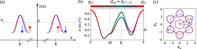
Figure 1: (a) Schematic representation of spin splitting of bands in TMD monolayers at the $K$ and $K^{\prime}$ points due to Ising SOC. (b) Low-energy orbital resolved electronic structure of monolayer NbSe₂. (c) Spin-resolved Fermi surface in the presence of Ising SOC. The results shown in (b) and (c) are obtained form relativistic DFT calculations.

Monolayer NbSe₂ is a prime candidate where Ising superconductivity can be studied. Bulk NbSe₂ has been extensively investigated experimentally and the transition at $T_{\mathrm{c}}\sim 7$K into the superconducting state is believed to be driven by strong electron-phonon coupling [38, 39, 40] with a superconducting gap corresponding to an $s$-wave symmetry. On the other hand, as the number of Nb layers is reduced, the transition temperature drops, and in monolayer NbSe₂, the superconducting state is observed only below $T_{c}\sim 3$ K [1, 41, 42, 5]. This suppression of $T_{\mathrm{c}}$ from the bulk to monolayer can be due to the enhancement of thermally driven superconducting phase fluctuations and the weakening of the strength of Cooper pairing in 2D. An additional possible factor contributing to this weakening is the expected reduced screening of the Coulomb interactions.

The pairing mechanism in monolayer NbSe₂ is, however, not well understood. A number of proposals have considered electron-phonon mediated superconducting pairing [43, 44, 4, 45, 46], while other models consider pairing arising from purely repulsive interactions [47, 48, 49, 50, 51, 52, 53]. There are also proposals considering a combination of electron-phonon and spin-fluctuation mediated pairing  [43]. A study of the electric field effect on superconductivity in monolayer NbSe₂ hints at a transition from a weak-coupling to a strong-coupling superconductor as the single crystal is thinned to the atomic length scale [41]. STM experiments indicate the presence of bosonic, undamped collective modes that could suggest the important role of spin fluctuations [28]. The presence of strong spin fluctuations has also been supported by an enhanced paramagnetic susceptibility extracted from DFT calculations [43]. The possibility of an unconventional superconducting order has also been ascribed to studies of magnetoresistance [54, 55] that suggest a two-fold symmetric anisotropic superconducting gap and non-monotonic behavior of $T_{\mathrm{c}}$ with increasing disorder concentrations [56, 57].

Motivated by these observations suggesting possible unconventional superconducting pairing and relevance of spin fluctuations in monolayer NbSe₂, we study the leading superconducting instabilities in monolayer NbSe₂ within the assumption that the pairing is mediated solely by spin and charge fluctuations. Previous works addressing Ising superconductivity from a repulsive pairing scenario have considered dominant pairing channels and symmetry arguments to obtain the superconducting gap symmetry [58, 8, 29, 59, 60, 61, 62, 63, 53]. Here, we develop a general framework incorporating Ising SOC and the multi-orbital nature in the electronic structure, and calculate the pairing kernel within a full-fledged multi-orbital spin- and charge-fluctuation formalism [64, 65, 66, 67, 68, 69]. We solve the associated linearized gap equation to obtain the leading superconducting order parameter and study the variation in solutions both as a function of SOC and Coulomb interaction strength. This leads to interesting regimes for the mixing between even- and odd-parity superconducting solutions. To identify the effect of the solution on measurable quantities, we next study the effect of an in-plane and out-of-plane magnetic field on $T_{\mathrm{c}}$ by solving the corresponding gap equations. Our work paves the way for a deeper understanding of the consequences of unconventional pairing in monolayer TMDs, and offers valuable insight into the interplay between Ising superconductivity with allowed singlet-triplet mixing and unique magnetic field dependence.
This paper is organized as follows: In Sec. II, we provide a description of the applied model Hamiltonian and our calculations of the relevant susceptibilities. In Sec. III, we derive the pairing kernel and solve the associated gap equation to infer the preferred superconducting states for monolayer Ising superconductors. In Sec. IV we discuss the effects of out-of-plane and in-plane magnetic fields. Finally, in Sec. V, we conclude and give a summary of our work. The associated Supplementary Material (SM) contains additional technical details.

II Model and Methodology

II.1 Hamiltonian

The lattice structure of monolayer NbSe₂ consists of a hexagonal lattice of Nb atoms sandwiched between Se atoms above and below the Nb plane. The arrangement of the Se atoms leads to broken inversion symmetry, but retains the $\mathcal{M}_{xy}$ mirror plane. As we reduce the number of layers, the point group symmetry of the crystal reduces from a D_6h symmetry (with inversion) relevant to the bulk material, to a D_3h symmetry (without inversion) in the monolayer. In the presence of Ising SOC, the eigenstates of $S_{z}$ remain good spin quantum numbers, and the SOC preferentially orients the spins to be along the $z$-axis i.e., out of the Nb plane. In the following, we utilize a multi-orbital tight-binding Hamiltonian to describe the low-energy electronic structure of monolayer NbSe₂

$$H_{\rm TB}=\sum_{\mathbf{k}l_{1}l_{2}\sigma}h_{l_{1}l_{2}\sigma}(\mathbf{k})c^{\dagger}_{\mathbf{k}l_{1}\sigma}c_{\mathbf{k}l_{2}\sigma}.$$ (1)

Here, $c^{\dagger}_{\mathbf{k}l\sigma}$ creates an electron with spin-$\sigma$, orbital $l$, and wavevector $\mathbf{k}$. The Hamiltonian matrix with components $h_{l_{1}l_{2}\sigma}(\mathbf{k})$ from Eq. (1) can be expressed as a $6\times 6$ block diagonal matrix due to the absence of spin-flip terms in the SOC. The above Hamiltonian can be represented in the band basis by performing a unitary transformation

$$c_{\mathbf{k},\tilde{l}}=\sum_{\alpha}u^{\alpha}_{\tilde{l}}(\mathbf{k})a_{\mathbf{k}\alpha\sigma},$$ (2)

where $u^{\alpha}_{\tilde{l}}(\mathbf{k})$ are components of the eigenvector corresponding to band $\alpha$ and we have used a compact notation $[\tilde{l}:=(l,\sigma)]$. In Fig. 1(b) we show the bands crossing the Fermi level together with the orbital content, highlighting that the Fermi surface exhibits regions where each of the three orbitals dominates. The model has been extracted from a DFT calculation using the full-potential local-orbital (FPLO) code [70], version 18.00-52 where a monolayer NbSe₂ was set up with the lattice constants $a=b=3.44\mathrm{\AA{}}$ and $c=12.48\mathrm{\AA{}}$ to simulate a vacuum. The space group is # 187, i.e. P-6m2 with the Nb at the origin and the Se atom at $(1/3,-1/3,0.1322)$. We employed the nonrelativistic setting for the band structure without SOC and the fully relativistic setting to obtain the effects of Ising SOC. The Wannier projection was performed onto the three orbitals $d_{z^{2}}$, $d_{x^{2}-y^{2}}$, $d_{xy}$ with energy window of $[-0.4,3.5]\,\mathrm{eV}$.

We find that a minimal model consisting of three Nb orbitals $(d_{z^{2}},d_{x^{2}-y^{2}},d_{xy})$ reproduces well the DFT-generated electronic structure. The low-energy electronic structure yields a single electronic band forming the Fermi surface that splits into two spin momentum locked bands in the presence of Ising SOC of strength $\delta_{\mathbf{k}}^{max}\sim 100$meV, in agreement with previous studies [71, 72]. Note that the SOC is not used as a tuning parameter in our study, but the two electronic structures considered in this work: with SOC and without SOC are both derived from DFT calculations as described above. (More details on the electronic structure are presented in Sec-I of the SM.)

As shown in Fig. 1(a), the two low-energy bands forming the Fermi surface can be described by eigenstates $|\mathbf{k},\uparrow\rangle$, and another band that enforces Kramers degeneracy with eigenstate $|-\mathbf{k},\downarrow\rangle$. Both bands contain contributions from all three $d$-orbitals, and each band is described additionally by a particular spin eigenstate due to spin momentum locking. As seen in Fig. 1(b), the $d_{z^{2}}$ orbital dominates the orbital content of the $\Gamma$-centered Fermi pockets, whereas the $K$ and $K^{\prime}$ centered pockets are dominated by the $d_{x^{2}-y^{2}}$ and $d_{xy}$ orbitals. In Fig. 1(c) we display the spin-resolved Fermi surface for monolayer NbSe₂ in the presence of Ising SOC. The presence of a horizontal mirror plane in the $xz$ plane ensures that the SOC and the band splitting vanishes along the $\Gamma-$M directions.

The bare electronic repulsion is given by the usual on-site Hubbard-Hund interaction, parametrized by $U$ and $J$. In a compact notation restricted to the Cooper channel, this interaction takes the form of (details given in SM)

$$H_{\rm int}=\frac{1}{2}\sum_{\mathbf{k},\mathbf{k}^{\prime},\tilde{l}}[U]^{\tilde{l}_{1},\tilde{l}_{2}}_{\tilde{l}_{3},\tilde{l}_{4}}\,c^{\dagger}_{\mathbf{k},\tilde{l}_{1}}\,c^{\dagger}_{-\mathbf{k},\tilde{l}_{3}}\,c_{-\mathbf{k}^{\prime},\tilde{l}_{2}}\,c_{\mathbf{k}^{\prime},\tilde{l}_{4}}.$$ (3)

Thus, the total Hamiltonian applied in the following analysis is given by

$$H=H_{\rm TB}+H_{\rm int}\,.$$ (4)

II.2 Calculation of Susceptibility

Computation of the spin and charge susceptibilities allows to extract the structure of the dominant spin and charge fluctuations, which in turn dictate the superconducting pairing within the present approach. The multi-orbital non-interacting bare susceptibility tensor at momentum ${\mathbf{q}}$ is defined as

$$\chi_{\tilde{l}_{3}\tilde{l}_{4}}^{\tilde{l}_{1}\tilde{l}_{2}}(\mathbf{q},\tau)\!=\!\!\frac{1}{N}\sum_{\mathbf{k},\mathbf{k}^{\prime}} \langle T_{\tau}\,c^{\dagger}_{\mathbf{k},\tilde{l}_{1}}(\tau)c_{\mathbf{k}+\mathbf{q},\tilde{l}_{2}}(\tau)c^{\dagger}_{\mathbf{k}^{\prime},\tilde{l}_{3}}(0)c_{\mathbf{k}^{\prime}-\mathbf{q},\tilde{l}_{4}}(0)\rangle_{0}.$$ (5)

Explicitly, this is given by

$$\chi_{\tilde{l}_{3}\tilde{l}_{4}}^{\tilde{l}_{1}\tilde{l}_{2}}(\mathbf{q},i\omega_{n}) =\frac{1}{N}\sum_{\mathbf{k},\alpha,\beta}\frac{f(\epsilon_{\beta}(\mathbf{k}+\mathbf{q}))-f(\epsilon_{\alpha}(\mathbf{k}))}{i\omega_{n}+\epsilon_{\alpha}(\mathbf{k})-\epsilon_{\beta}(\mathbf{k}+\mathbf{q})}$$

$$\times u^{\alpha}_{\tilde{l}_{4}}(\mathbf{k})u^{\alpha*}_{\tilde{l}_{1}}(\mathbf{k})u^{\beta}_{\tilde{l}_{2}}(\mathbf{k}+\mathbf{q})u^{\beta*}_{\tilde{l}_{3}}(\mathbf{k}+\mathbf{q}).$$ (6)

The eigenenergies $\epsilon_{\alpha}(\mathbf{k})$ are calculated at momentum $\mathbf{k}$ and belong to band $\alpha=(1,\ldots,6)$, and the function $f(x)=(1+e^{\beta x})^{-1}$ with $\beta=1/{k_{B}T}$ denotes the Fermi-Dirac distribution function at temperature $T$.

From Eq. (6) we perform an analytical continuation $i\omega_{n}\rightarrow\omega+i\eta$ and evaluate the multi-orbital susceptibility by summing over a $k$-grid in the Brillouin zone (BZ) and take interactions into account via the random phase approximation (RPA), see SM for details. In Fig. 2, we show the physical paramagnetic susceptibility extracted from the multi-orbital susceptibility. To extract the physical susceptibility from $\chi_{\tilde{l}_{3}\tilde{l}_{4}}^{\tilde{l}_{1}\tilde{l}_{2}}(\mathbf{q},i\omega_{n})$ we consider the orbital components having $l_{1}=l_{2}$, and $l_{3}=l_{4}$ and sum over the orbitals. Then the physical susceptibility in the longitudinal ($\chi^{l}$) and transverse ($\chi^{t}$) channels can be expressed as

$$\chi^{l}(\mathbf{q},\omega) = \frac{1}{4}(\chi_{\uparrow\uparrow}^{\uparrow\uparrow}-\chi_{\downarrow\downarrow}^{\uparrow\uparrow}-\chi_{\uparrow\uparrow}^{\downarrow\downarrow}+\chi_{\downarrow\downarrow}^{\downarrow\downarrow}),$$ (7)

$$\chi^{t}(\mathbf{q},\omega) = \frac{1}{2}(\chi_{\downarrow\uparrow}^{\uparrow\downarrow}+\chi_{\uparrow\downarrow}^{\downarrow\uparrow}),$$ (8)

where, for ease of notation, we have suppressed the orbital indices that are being summed over.

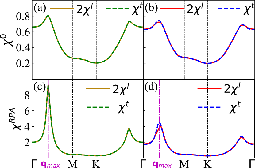
Figure 2: Spin susceptibility at $\omega=0$ along the high-symmetry path $\Gamma$-$M$-$K$-$\Gamma$. (a) and (c) display the non-interacting and RPA susceptibilities, respectively, calculated without SOC. (b) and (d) display these same quantities in the presence of Ising SOC. For both cases the RPA paramagnetic susceptibility peak occurs at a wave vector $\mathbf{q}_{\mathrm{max}}\sim 0.4$$\Gamma-$M. For the RPA susceptibility, we used $U=1.0,J=U/4$.

The paramagnetic susceptibility peaks at a wave vector $\mathbf{q}_{\mathrm{max}}\sim 0.4$$\Gamma-$M, which agrees with previous calculations from a DFT-derived band structure [33, 47, 48]. Experimentally, a 3Q CDW order is observed in monolayer NbSe₂ which corresponds to a wave vector of $\mathbf{q}_{\mathrm{CDW}}\sim 2/3\Gamma-$M along the three symmetry-related directions [73], implying that a pure nesting-driven scenario cannot explain the formation of CDW in this material. Therefore, it is likely that additional effects, such as electron-phonon interactions, need to be accounted for in order to understand the CDW phase in monolayer NbSe₂. A similar electron-phonon interaction effect has been used to explain the formation of 3Q CDW state in bulk bilayer 2H$-$NbSe₂ [74, 75, 76].

In the presence of Ising SOC, the susceptibility is calculated in a basis where the Ising SOC induced spin momentum locking and corresponding spin splitting of electronic bands is taken into account. In Fig. 2(c) and Fig. 2(d), we show the non-interacting and RPA susceptibilities in the presence of Ising SOC, respectively. The non-interacting susceptibility is slightly reduced upon the inclusion of Ising SOC, although the maximum peak remains at $\mathbf{q}_{\mathrm{max}}$. As expected, the SOC leads to a breaking of the degeneracy between the transverse and longitudinal channels. It turns out that in the presence of Ising SOC, the transverse susceptibility is enhanced compared to the longitudinal susceptibility, an effect that is much stronger in the interacting RPA susceptibilities. In the following section we show that such enhancement causes the interchange in the role of dominant even-parity superconducting instability and subdominant odd-parity instability. As the enhancement increases as a function of Coulomb interaction $U$, the odd-parity solution becomes the favorable state.

III Leading Superconducting Instabilities

Within a spin fluctuation-mediated pairing scenario, the effective superconducting pairing kernel has to incorporate the mixing of spin and orbital indices induced by the SOC [68]. The pairing kernel can be expressed as

$$[V(\mathbf{k},\mathbf{k}^{\prime})]^{\tilde{l}_{1},\tilde{l}_{2}}_{\tilde{l}_{3},\tilde{l}_{4}} = [U]^{\tilde{l}_{1},\tilde{l}_{2}}_{\tilde{l}_{3},\tilde{l}_{4}}-[\frac{U\,\chi_{0}\,U}{1-\chi_{0}\,U}]^{\tilde{l}_{1},\tilde{l}_{4}}_{\tilde{l}_{3},\tilde{l}_{2}}(\mathbf{k}-\mathbf{k}^{\prime})$$ (9)

$$+ [\frac{U\,\chi_{0}\,U}{1-\chi_{0}\,U}]^{\tilde{l}_{1},\tilde{l}_{2}}_{\tilde{l}_{3},\tilde{l}_{4}}(\mathbf{k}+\mathbf{k}^{\prime}).$$

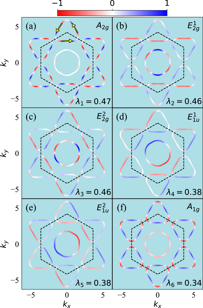
Figure 3: Solutions of the linearized gap equation $\Delta(\mathbf{k}_{F})$ plotted on the Fermi surface for the six leading superconducting pairing gaps with corresponding eigenvalue $\lambda$. The non-interacting Hamiltonian used here ignores the Ising SOC. Additional parameters: $U=1.0$, $J=U/4$.

The interaction matrix $U$ and the individual contributions to the pairing kernel are provided in the SM. The superconducting gap function is defined as

$$\Delta^{\tilde{m}_{1},\tilde{m}_{2}}(\mathbf{k})=-\sum_{\mathbf{p},\tilde{m}_{3},\tilde{m}_{4}}V^{\tilde{m}_{2},\tilde{m}_{1}}_{\tilde{m}_{3},\tilde{m}_{4}}(\mathbf{k},\mathbf{k}^{\prime})\langle a_{\mathbf{k},\tilde{m}_{3}}(\tau)a_{-\mathbf{k}^{\prime},\tilde{m}_{4}}(\tau)\rangle,$$ (10)

where $V_{\tilde{m}_{3},\tilde{m}_{4}}^{\tilde{m}_{1},\tilde{m}_{2}}(\mathbf{k},\mathbf{k}^{\prime})$ is the pairing interaction projected on the Fermi surface. The indices $[\tilde{m}_{i}:=(m_{i},\sigma_{i})]$ represent the band indices and the spin degrees of freedom, respectively; $m_{i}$ takes the values $(1,2,3)$ and $\sigma_{i}$ takes the values $(1,2)$.

The linearized gap equation in the presence of Ising SOC can be derived from the Gor’kov Green’s functions (see SM Sec-III). For a two-band system with bands relevant to monolayer NbSe₂, the gap equation can be expressed as

$$\Delta^{\tilde{m},\tilde{m}^{\prime}}(\mathbf{k})=-\tilde{I} \sum_{\begin{subarray}{c}\mathbf{k}^{\prime}\end{subarray}}\left[V^{\tilde{m}^{\prime},\tilde{m}}_{\tilde{m},\tilde{m}^{\prime}}(\mathbf{k},\mathbf{k}^{\prime})\Delta^{\tilde{m},\tilde{m}^{\prime}}(\mathbf{k}^{\prime})\right.$$

$$\left.+V^{\tilde{m}^{\prime},\tilde{m}}_{\tilde{m}^{\prime},\tilde{m}}(\mathbf{k},\mathbf{k}^{\prime})\Delta^{\tilde{m}^{\prime},\tilde{m}}(\mathbf{k}^{\prime})\right],$$ (11)

where $\tilde{I}=\text{ln}\left(\frac{2e^{\gamma}\hbar\omega_{\mathrm{c}}}{\pi k_{B}T_{\mathrm{c}}}\right)$. Here the gap equation is restricted to the opposite spin pairing states with $\tilde{m}=(m,\sigma)$, and $\tilde{m}^{\prime}=(m^{\prime},\bar{\sigma})$. A zero energy and a zero momentum gap function $\Delta^{\tilde{m},\tilde{m}^{\prime}}(\mathbf{k})$ pairs opposite spin states, i.e. with different $\tilde{m}\neq\tilde{m}^{\prime}$, but originating from the same $m$.

III.1 Gap solutions without Ising SOC

Figure 3 displays the solutions of the linearized gap equation for $U=1$ eV and in the absence of SOC where the underlying symmetry of the gap functions belongs to the irreducible representations (irrep) of D_6h point group. The ground state superconducting gap belongs to an irrep of the even-parity A_2g representation with gap nodes along the $\Gamma-$K directions. The dominance of the observed nodal pairing structure can be attributed to the nesting properties of the Fermi surface. As shown in Fig. 2, the peak in the susceptibility occurs around 0.4$\Gamma$M. This momentum vector corresponds to the intra-pocket nesting vectors depicted by the yellow arrows in Fig. 3(a) (see also Sec-IV of SM for more details). We also find that the dominant A_2g symmetry superconducting gap on the $\Gamma$-centered Fermi pocket is much smaller than the gap magnitude on the $K$-centered pockets. The subleading gap functions are a set of degenerate states that belong to the two-dimensional (2D) E_2g irrep (Fig. 3(b,c)) with basis functions ($f_{k_{x^{2}}-k_{y^{2}}}$,$f_{k_{x}k_{y}}$) followed by the odd-parity solutions belonging to the 2D E_1u irrep (Fig. 3(d,e)) with basis functions $(f_{k_{x}},f_{k_{y}})$. In fact, as seen from Fig. 4(a), the gap functions belonging to these three states remain quite close in energy with variation in Coulomb interaction.

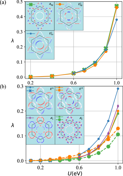
Figure 4: (a) Evolution of eigenvalues $\lambda$, associated with a given superconducting gap function as a function of $U$ with $J=U/4$ in the absence of Ising SOC. (b) Evolution of the eigenvalue $\lambda$, associated with a given superconducting gap function as a function of $U$ in the presence of Ising SOC. The solid lines correspond to $J=U/4$, and the dashed lines correspond to $J=U/6$, respectively. The inset gap solutions displayed have the same color bar as Fig. 3. Note that for $U<0.6$, E^′1 and A${}_{1}^{\prime}$ solutions have much smaller eigenvalue, and hence are not visible in the plot.

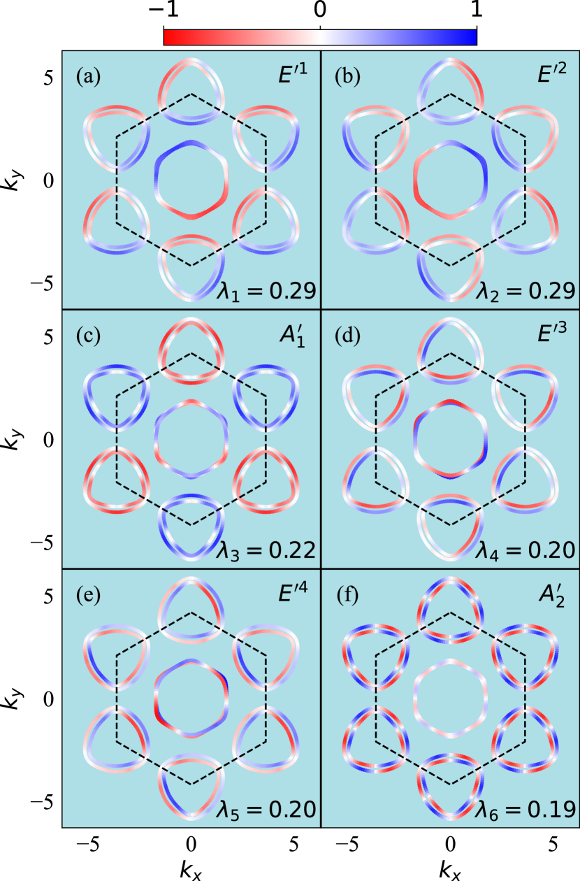
Figure 5: Superconducting gap functions plotted on Fermi surface in the presence of Ising SOC with $U=1.0$, $J=U/4$. Here, $\lambda$ on the plots denote the eigenvalues of the corresponding solutions of the gap equation. Panels (a) and (b) display the degenerate ground state solution.

III.2 Gap solutions with Ising SOC

Next, we consider the pairing in the presence of Ising SOC. Previous studies considering a repulsive pairing interaction have proposed a leading superconducting instability in the $s+f$-wave channel [53, 77, 78, 63, 79]. In Fig. 4(b) we show the evolution of the various gap function symmetries with variation in Coulomb interaction. In order to focus on the detailed momentum space structure of the gap function, in Fig. 5 we present the solutions of the linearized gap equation in the presence of Ising SOC for $U=1$ eV, and $J=0.25U$.

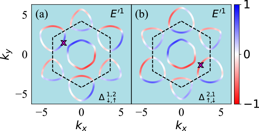
Figure 6: The ground state superconducting gap function displayed separately on the spin-up (a) and spin-down (b) Fermi surfaces. The solution on the Fermi pocket on the two bands are related by $\Delta^{1,2}_{\uparrow,\downarrow}(\mathbf{k})=-\Delta^{2,1}_{\downarrow,\uparrow}(-\mathbf{k})$. Here, $U=1$, $J=U/4$ and $\lambda=0.29$.

In the following, the notation for band indices $\tilde{m}=(1,2)$ correspond to bands with definite spin eigenstates $(\uparrow,\downarrow)$ respectively. From Fig. 5 it is apparent that the ground state superconducting gap solution exhibits a degeneracy between the first two obtained eigenvalues (see Fig. 5(a,b)), and belongs to the 2D E^′ irrep of the D_3h point group. We also find from Fig. 4(b) that this solution remains the stable ground state solution with variation in Coulomb interaction. In the presence of broken inversion symmetry, this solution mixes even- and odd-parity states corresponding to basis functions of E_2g and E_1u symmetry of the D_6h point group, although as discussed below the odd-parity contribution dominates the mixed state for stronger Coulomb interactions. This result deviates from the corresponding solution in absence of SOC where the ground state superconducting solution is an even-parity A_2g ($i$ wave) state whereas the A${}_{2}^{\prime}$ symmetry superconducting state (A_2g+B_2u or $i+f$) is a subdominant order in the presence of SOC (see Fig. 5(f)). We also find that the superconducting gap on the $\Gamma$-centered pocket is relatively larger in the presence of Ising SOC and becomes comparable to the gap on the $K$-centered pockets for the dominant E₂ as well as the subdominant A₁ representations. These results are supported by the corresponding nesting vectors for the spin-split Fermi surface. The dominant nesting in the presence of Ising SOC connects additional inter-pocket regions between the $K$ and $K^{\prime}$ points as well as regions between the $\Gamma$-pocket and the $K$-pockets, which is the likely reason for the enhanced superconducting gap on the $\Gamma$ pocket in the presence of SOC. (see Sec-IV of SM for further details). Further, considering a model where we only include the Ising SOC in the electronic band structure and not in the superconducting pairing kernel, we find that the ground state superconducting solution still exhibits dominant odd-parity state mixture. This implies that the spin-split band structure due to presence of the Ising SOC preferentially supports an odd-parity superconducting state.

The solution on the Fermi pocket on the two bands are related by $\Delta^{1,2}_{\uparrow,\downarrow}(\mathbf{k})=-\Delta^{2,1}_{\downarrow,\uparrow}(-\mathbf{k})$, see Fig. 6(a,b), which is required by the exclusion principle. In order to identify the superconducting gap symmetry and corresponding irrep from the gap structure, consider a $180^{\circ}$ rotation operation $\sigma_{v}$ about an in-plane axis slanted at an angle of $30^{\circ}$ from the k_x direction that we call the k${}_{x}^{\prime}$ direction. If we express the rotated coordinate system in a $(k_{x}^{\prime},k_{y}^{\prime})$ basis, then $k_{x}^{\prime}=(\sqrt{3}k_{x}+k_{y})/2$, and $k_{y}^{\prime}=(-k_{x}+\sqrt{3}k_{y})/2$. Therefore, since from Fig. 6(a,b) $\sigma_{v}\Delta(k_{x}^{\prime},k_{y}^{\prime})=\Delta(k_{x}^{\prime},-k_{y}^{\prime})=-\Delta(k_{x}^{\prime},k_{y}^{\prime})$, we have a node at $\Delta(k_{x}^{\prime},0)$. This transformation of the gap function under a symmetry operation of the D_3h point group combined with the presence of a degenerate superconducting state in the solution of the linearized gap equation, ensures that the corresponding gap function belongs to the E^′ irrep. In fact, the gap function can be expressed as $\Delta(\mathbf{k})\sim af_{k_{x}^{\prime}k_{y}^{\prime}}+bf_{k_{y}^{\prime}}$, where $a$, and $b$ are constant numbers. In the original $(k_{x},k_{y})$ basis, the other components of the 2D irrep will of course get mixed, but determining the specific mixing that minimizes the ground state energy would require the theory to be extended beyond a linearized gap equation.

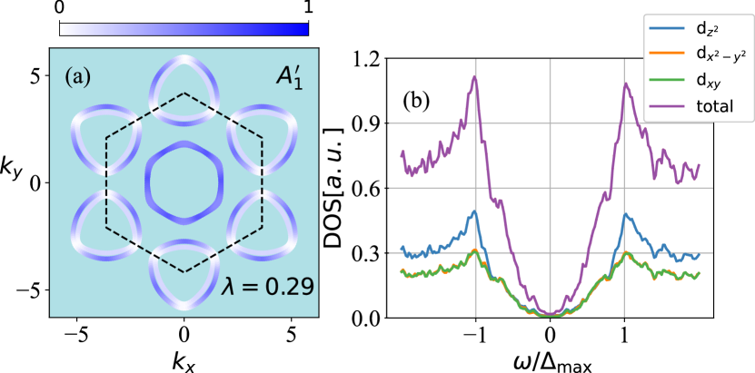
Figure 7: (a) $|\Delta_{1}(\mathbf{k})+i\Delta_{2}(\mathbf{k})|^{2}$ plotted on the Fermi surface pockets. Here $\Delta_{1}(\mathbf{k})$, and $\Delta_{2}(\mathbf{k})$ are the two degenerate leading superconducting gap functions shown in Fig. 5(a,b) for the case with Ising SOC. (b) Orbital-resolved DOS corresponding to the solution $\Delta_{1}(\mathbf{k})+i\Delta_{2}(\mathbf{k})$.

It is instructive to consider the structure of $|\Delta_{1}(\mathbf{k})+i\Delta_{2}(\mathbf{k})|^{2}$ where $\Delta_{1}(\mathbf{k})$, and $\Delta_{2}(\mathbf{k})$ are the degenerate superconducting ground state solutions represented in Fig. 5(a,b). This complex superposition is the expected $T=0$ state due to its minimization of the condensation energy, as compared to the individual solutions. As shown in Fig. 7(a), the magnitude of this $(1,i)$ state belongs to an A^′ representation of the D_3h point group symmetry as expected from the decomposition of the reducible representation $\Gamma_{E^{\prime}}\times\Gamma_{E^{\prime}}^{*}$. The anisotropy of the gap structure leads to a multigap feature and a density of states (DOS) that displays a U-shaped form at low energies (see Fig. 7(b))[80]. Although, these multigap features in the DOS would presumably be further influenced by the presence of an underlying CDW ordering, it is interesting to note that similar multigap features and a low-energy U-shaped DOS have been observed in low-temperature STM measurements on ultra-thin films of NbSe₂[23].

III.3 Singlet-Triplet mixing

We can approximately quantify the singlet-triplet mixing by considering the superconducting gaps $\Delta^{1,2}_{\uparrow\downarrow}(\mathbf{k})=\Delta^{1,2}(\mathbf{k}+\delta_{\mathbf{k}}/2)$ on the spin-up Fermi surface and $\Delta^{2,1}_{\downarrow\uparrow}(\mathbf{k})=\Delta^{2,1}(\mathbf{k}-\delta_{\mathbf{k}}/2)$ on the spin-down Fermi surface. At every Fermi wave vector $\mathbf{k}$ corresponding to the Fermi surface without SOC, we define a $\delta_{\mathbf{k}}$ representing half of the corresponding band splitting when SOC is introduced. Then $\mathbf{k}\pm\delta_{\mathbf{k}}$ are approximately (the splitting, in general, will not be symmetrical) the Fermi wave vectors for the two spin-split bands. We then define the even- and odd-parity gaps as $\Delta_{o/e}(\mathbf{k})=\Delta^{1,2}_{\uparrow\downarrow}(\mathbf{k})\pm\Delta^{2,1}_{\downarrow\uparrow}(\mathbf{k})$, and the quantity $\eta=\sum_{\mathbf{k}}\frac{|\Delta_{e}(\mathbf{k})|-|\Delta_{o}(\mathbf{k})|}{|\Delta_{e}(\mathbf{k})|+|\Delta_{o}(\mathbf{k})|}$, as a measure of the singlet-triplet mixing ratio. In Fig. 8, the variation of the mixing ratio $\eta$ of the ground state gap function reveals that the odd-parity superconducting state dominates the mixed state for larger Coulomb interactions.

The observation of superconducting collective modes in tunneling experiments have been interpreted either as a Leggett mode between an s-wave state and a proximate f-wave channel  [28] or as a fluctuation of the superconducting order parameter phase between the $K$ and $\Gamma$ pocket induced by a strong suppression in gap over the $\Gamma$ pocket [43]. Although our result does not find either a dominant $s+f$ gap structure, or strong anisotropy of the gap magnitude between the $K$ and $\Gamma$ pockets, we do find that within a spin-fluctuation-mediated pairing mechanism a significant mixing of even- and odd-parity superconducting states occur, and this could lead to a Leggett mode between an E_1g and a proximate E_1u odd-parity channel.

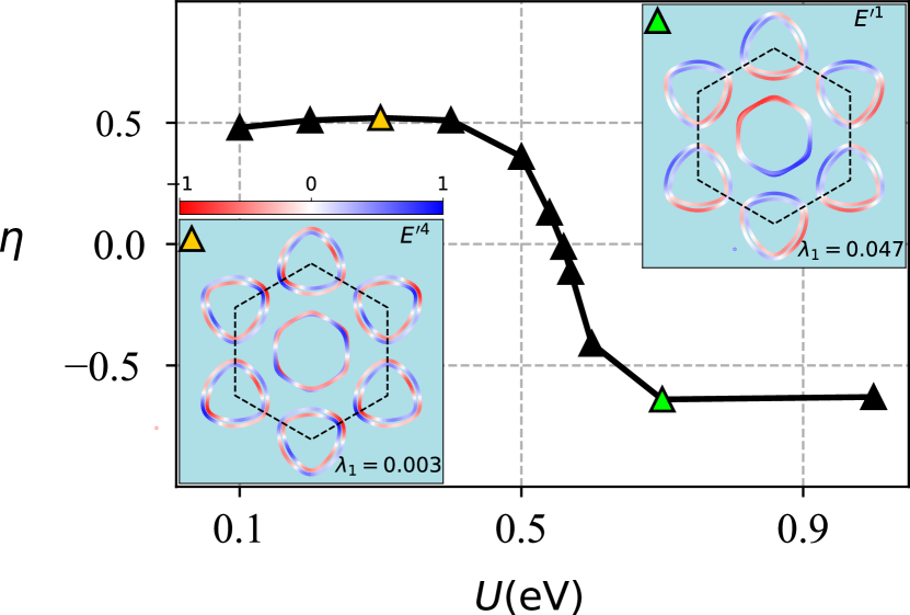
Figure 8: Superconducting singlet-triplet mixing ratio $\eta$ as a function of the Coulomb interaction $U$ with $J=U/4$. $\eta=(+1)(-1)$ corresponds to the pure even(odd) parity solutions. The gap solutions displayed in the two insets have the same color bar as Fig. 3.

IV Magnetic Field Effect

The presence of Ising SOC and the resulting mixing of even- and odd-parity gap functions in TMD superconductors lead to a non-trivial dependence of the superconducting gap function on a magnetic field. The general Hamiltonian for the Zeeman term with arbitrary field direction can be written as

$$H_{\mathrm{Zeeman}}=g\mu_{B}\sum_{l,\mathbf{k},\sigma,\sigma^{\prime}}\left[\boldsymbol{\sigma}\cdot\mathbf{B}\right]_{\sigma\sigma^{\prime}}c^{\dagger}_{\mathbf{k}l\sigma}c_{\mathbf{k}l\sigma^{\prime}}.$$ (12)

Here, $\boldsymbol{\sigma}\equiv(\sigma_{x},\sigma_{y},\sigma_{z})$ denotes a vector of Pauli matrices and $\mathbf{B}\equiv(B_{x},B_{y},B_{z})$ originates from an applied magnetic field.

IV.1 Out-of-plane magnetic field

We first study the effect of a longitudinal magnetic field on superconducting monolayer NbSe₂ ignoring any orbital effect and considering only the Pauli paramagnetic contribution within the superconducting state. The Zeeman field Hamiltonian is given by

$$H_{B_{z}}=g\mu_{B}B_{z}\sum_{l,\mathbf{k}}(n_{\mathbf{k}l\uparrow}-n_{\mathbf{k}l\downarrow}),$$ (13)

where $n_{\mathbf{k}l\sigma}=c^{{\dagger}}_{\mathbf{k}l\sigma}c_{\mathbf{k}l\sigma}$. Since the non-interacting Hamiltonian exhibits no spin-flip contributions, the above term preserves $S_{z}$ as a good quantum number. We consider the magnetic field as a perturbation and obtain the homogeneous solution of the linearized gap equation (see SM for further details). This leads to a second-order transition curve similar to earlier studies [81]. Further, as shown in Fig. 9, we do not find any appreciable effect of the Ising SOC on the second-order phase transition curve in the case of out-of-plane magnetic fields.

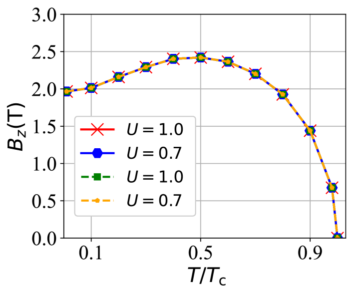
Figure 9: Effect of an out-of-plane magnetic field on $T/T_{c}$ for various $U$. Solid lines are obtained the presence of Ising SOC, and dashed lines are obtained in the absence of Ising SOC, respectively.

IV.2 In-plane magnetic field

For an in-plane magnetic field in a 2D material, the presence of a spin-flip term implies that $S_{z}$ is no longer a good quantum number. In this case, for a field in the $x$ direction, the Zeeman term contribution can be expressed as

$$H_{B_{x}}=g\mu_{B}B_{x}\sum_{\mathbf{k},l}(c^{{\dagger}}_{\mathbf{k}l\uparrow}c_{\mathbf{k}l\downarrow}+c^{{\dagger}}_{\mathbf{k}l\downarrow}c_{\mathbf{k}l\uparrow}).$$ (14)

In the following, we consider the in-plane magnetic field as a perturbation and represent it in the band basis of the non-interacting Hamiltonian. This results in a Hamiltonian of the form

$$H_{B_{x}}=\sum_{mm^{\prime}\mathbf{k}}\left(h_{\mathbf{k}\uparrow\downarrow}^{m,m^{\prime}}a_{\mathbf{k}m\uparrow}^{{\dagger}}a_{\mathbf{k}m^{\prime}\downarrow}+\mbox{H.c}\right).$$ (15)

Here, $h_{\mathbf{k}\sigma\bar{\sigma}}^{m,m^{\prime}}=g\mu_{B}B_{x}\sum_{\mu}u_{m\sigma}^{*\mu}(\mathbf{k})u_{m^{\prime}\bar{\sigma}}^{\mu}(\mathbf{k})$ and we have used the transformation in Eq. (2) in zero magnetic field, $m$ represents the band index running from 1 to 3. Due to spin-spitting, we get 6 effective bands, 3 corresponding to spin-up and the other 3 corresponding to spin-down. The orbital index $\mu$ also runs over three orbital components ($d_{z^{2}}$, $d_{x^{2}-y^{2}}$, $d_{xy}$). Since we ignore the effect of an in-plane magnetic field on the pairing kernel, our model does not consider the possibility of an equal-spin pairing gap induced by tilting of the spins from the out-of-plane direction induced by finite in-plane magnetic fields. However, as discussed in the SM, the presence of the in-plane Zeeman field leads to finite equal-spin superconducting correlations. Computationally, the resultant gap equation is numerically solved for each magnetic field value by fixing the superconducting transition temperature at zero field to $T_{\mathrm{c}}=3$ K. The linearized gap equation becomes

$$-\Delta^{\tilde{m},\tilde{m}^{\prime}}(\mathbf{k})= \sum_{\begin{subarray}{c}\mathbf{k}^{\prime}\end{subarray}}[\left(V^{\tilde{m}^{\prime},\tilde{m}}_{\tilde{m},\tilde{m}^{\prime}}(\mathbf{k},\mathbf{k}^{\prime})I_{1}(\mathbf{k}^{\prime})+V^{\tilde{m}^{\prime},\tilde{m}}_{\tilde{m}^{\prime},\tilde{m}}(\mathbf{k},\mathbf{k}^{\prime})I_{2}(\mathbf{k}^{\prime})\right)\Delta^{\tilde{m},\tilde{m}^{\prime}}(\mathbf{k}^{\prime})$$

$$+\left(V^{\tilde{m}^{\prime},\tilde{m}}_{\tilde{m}^{\prime},\tilde{m}}(\mathbf{k},\mathbf{k}^{\prime})I_{1}(\mathbf{k}^{\prime})+V^{\tilde{m}^{\prime},\tilde{m}}_{\tilde{m},\tilde{m}^{\prime}}(\mathbf{k},\mathbf{k}^{\prime})I_{2}(\mathbf{k}^{\prime})\right)\Delta^{\tilde{m}^{\prime},\tilde{m}}(\mathbf{k}^{\prime})],$$ (16)

where

$$I_{1} =-\text{ln}\left(\frac{T}{T_{\mathrm{c}}}\right)+\frac{1}{\lambda}$$

$$-\frac{1}{2}\left(\frac{-h_{\mathbf{k}}^{2}}{h_{\mathbf{k}}^{2}+\delta_{\mathbf{k}}^{2}}\right)\left[\mathrm{Re}[\psi(\frac{1}{2}+i\frac{\sqrt{h_{\mathbf{k}}^{2}+\delta_{\mathbf{k}}^{2}}}{2\pi k_{B}T})]-\psi(\frac{1}{2})\right],$$ (17a)

$$I_{2} =\frac{1}{2}\left(\frac{-h_{\mathbf{k}}^{2}}{h_{\mathbf{k}}^{2}+\delta_{\mathbf{k}}^{2}}\right)\left[\mathrm{Re}[\psi(\frac{1}{2}+i\frac{\sqrt{h_{\mathbf{k}}^{2}+\delta_{\mathbf{k}}^{2}}}{2\pi k_{B}T})]-\psi(\frac{1}{2})\right].$$ (17b)

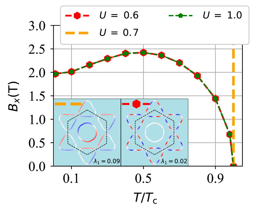
Figure 10: Effect of an in-plane magnetic field on $T/T_{\mathrm{c}}$ in the absence of SOC for various $U$. (Inset) Solutions corresponding to the highest eigenvalue for various $U$ in the absence of SOC. The inset gap solutions displayed have the same color bar as Fig. 3.

Here, $\psi$ denotes the digamma function. Further detailed steps can be found in the SM. Let us first consider the solution of the gap equation in the absence of Ising SOC. In this case, we retain the classification of the solution to even- and odd-parity channels, and the spin index on the eigenvector components can be suppressed without loss of generality. Then the orthonormality of the eigenvectors allows us to write $h_{\mathbf{k}\uparrow\downarrow}^{m,m^{\prime}}=h_{x}$. As can be seen from Fig. 10, in the absence of SOC, the triplet pairing is unaffected by an in-plane magnetic field, whereas the singlet state gets suppressed [82]. This behavior agrees with previous studies of magnetic field effects in spin-singlet and spin-triplet superconductors [81, 58, 78]. Note that the invariance of the transition temperature on the in-plane magnetic field for a triplet solution of monolayer NbSe₂ can be easily understood since the opposite-spin pairing triplet state implies that the $\mathbf{d}(\mathbf{k})$ vector is out of the plane. Therefore, the transition temperature, which depends on $|\mathbf{d}(\mathbf{k})\cdot\mathbf{B}|$, is independent of the magnetic field.

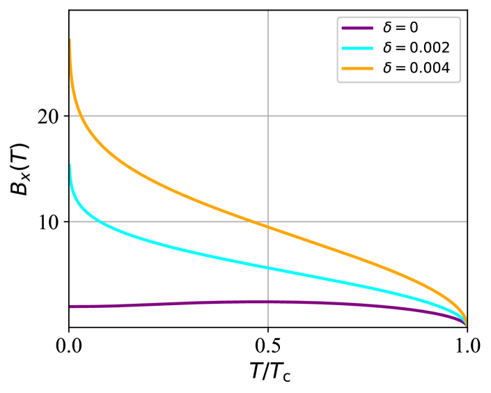
Figure 11: Effect of Ising SOC on $T/T_{\mathrm{c}}$ demonstrated in a simplified model, where we ignore the momentum-dependence of Ising SOC and consider an even-parity superconducting state obeying Eq. (18).

In the presence of Ising SOC, the results become non-trivial due to the mixing of momentum-dependent even- and odd-parity superconducting states and a momentum-dependent SOC. To identify the individual roles of the SOC and the parity of the superconducting state, we first consider a simplified case where we assume a spin-singlet gap function and ignore the momentum dependence of the Ising SOC and the in-plane magnetic field. In this approximation, the resulting gap equation allows us to decouple the transition temperature-dependent contribution from the gap matrix. The resulting equation is given by

$$\text{ln}\left(\frac{T}{T_{\mathrm{c}}}\right)=\frac{-h_{x}^{2}}{h_{x}^{2}+\delta^{2}}\Bigl{\{}\mathop{\mathrm{Re}}\Bigl{[}\psi\bigl{(}\frac{1}{2}+i\frac{\sqrt{h_{x}^{2}+\delta^{2}}}{2\pi k_{B}T}\bigr{)}\Bigr{]}-\psi\bigl{(}\frac{1}{2}\bigr{)}\Bigr{\}}.$$ (18)

The behavior of the above simplified model has been considered in previous works on monolayer TMDs [62, 83] and as shown in Fig. 11 leads to an enhancement of the upper critical field and a SOC-induced low-temperature upturn in the critical magnetic field. For odd-parity states, the transition temperature remains independent of magnetic fields. It is believed that a similar SOC-induced enhancement of the upper critical field explains the large upper critical fields in Ising superconductors compared to the Pauli limit. For example, monolayer TaS₂ with stronger Ising SOC compared to monolayer NbSe₂ exhibits a correspondingly larger critical field [26]. Additionally, the critical field is suppressed by increasing the number of layers in NbSe₂ [26]. This effect can be related to the weakening of Ising SOC due to cancellation of oppositely oriented internal magnetic fields from consecutive layers.

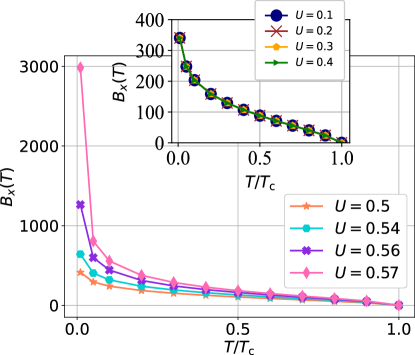
Figure 12: Effect of in-plane magnetic field on $T/T_{\mathrm{c}}$ in the presence of Ising SOC. Here, as opposed to the results shown in Fig. 11, we have taken into account the full momentum-dependence of the Ising SOC and the allowed mixing of even- and odd-parity superconducting states.

We next consider the numerical solution of the full linearized gap equation $(\ref{fullgapeqn})$ in the presence of momentum-dependent Ising SOC and mixed even- and odd-parity superconducting states. Note that with this generalization, the magnetic field and transition temperature cannot be decoupled from the gap matrix itself, and the self-consistent equation has to be numerically solved (see SM). In Fig. 12, the solution of the gap equation is shown for various values of onsite Hubbard interaction $U$ (and corresponding pairing interaction). As seen, the SOC significantly enhances the critical magnetic fields in the low-temperature limit with increasing $U$. For $U>0.6$ eV the transition temperature becomes independent of the magnetic field, indicating a superconducting state that is dominated by the odd-parity channel. This result agrees with the gap function obtained for $U=1.0$ eV shown in Fig. 5.

The low-temperature upturn in the second order transition line shown in Fig. 12 is much stronger than the upturn expected from a purely SOC effect considered in Fig. 11 for a spin-singlet system. The additional upturn is explained by the mixing of odd parity superconducting state. However, although a similar low-temperature upturn has been reported for Ising superconductors [34] and explained to be a consequence of Ising SOC, a large enhancement in the critical field has not been reported for monolayer NbSe₂. The suppression of an upturn in the critical field of Ising superconductors can originate via inhomogeneities or through the effect of competing orders. For example, it has been suggested that the presence of disorder can lead to an effective reduction in the SOC energy scale [84]. Therefore, disorder effects would not only suppress the superconducting gap, but the reduced SOC can also reduce the low-temperature upturn in critical magnetic fields. Additionally, the low-temperature upturn could also be suppressed by the presence of an additional Rashba SOC [84, 85] that could originate from a weak breaking of the in-plane mirror symmetry due to a substrate layer. A finite Rashba SOC contribution induces an in-plane spin component and reduces the protection of the superconducting state from in-plane magnetic fields.

Another interesting feature relevant to monolayer NbSe₂ is the underlying 3Q CDW order. Previous studies on this system have ignored the effect of CDW on the superconducting state since the CDW experimentally shows up only as a small anomaly in local DOS measurements, indicating the opening of an anisotropic CDW gap over small regions of the Fermi surface [5, 73]. Additionally, suppression of CDW by disorder or pressure seems to have only a rather small effect on the superconducting transition temperature [43, 5]. First principles calculations indicate that the CDW gap primarily opens up at the Fermi surface around the $K$, $K^{\prime}$ points [86]. However, if we note that these are also the regions where the momentum-dependent Ising SOC is large, the CDW will likely influence the superconducting pairing and lead to modification of low-temperature upturn in the critical magnetic field. Another important contribution of the underlying CDW phase could be to smear-out the two-gap feature obtained in the DOS.

V Summary

In summary, we have provided a theoretical framework to compute the effective momentum-dependent superconducting pairing interaction from repulsive interactions in Ising superconductors. The pairing is obtained from charge- and spin-fluctuation diagrams and incorporates the full momentum-dependence of the band structure and the Ising SOC. While this formalism is not established as the method for pairing from repulsive interaction, it is nevertheless well studied and has successfully described $d_{x^{2}-y^{2}}$ superconductivity in cuprates and $s^{\pm}$ superconducting order in the iron-based superconductors [87, 88, 89, 90, 91, 92]. We have applied this formalism to the case of monolayer NbSe₂ and explored the consequences of unconventional superconductivity in this material. We find that a reliable description of the preferred superconducting state depends crucially on the inclusion of all relevant Fermi pockets and the Ising SOC. Additionally, the solutions of the superconducting gap equation exhibit a significant dependence of the onsite Coulomb interaction, which determines the degree of mixing of even- and odd-parity superconducting states. While the odd-parity solutions exist as subdominant order parameters in the absence of Ising SOC, they become a dominant part of the leading gap structure in the presence of realistic amplitudes of Ising SOC. We have also studied the effect of the Hund’s coupling parameter $J$, revealing that an enhancement of $J$ results in a further dominance of the odd-parity channel in the mixing. These results highlight monolayer TMDs as interesting potential candidates for realising the interesting phenomenology of spin-triplet superconductivity, see also Refs. 51, 93.

The detailed momentum dependence of the gap structure obtained within the present approach, depends strongly on the inclusion of Ising SOC and the strength of the interactions. In the realistic cases, the $\Gamma$-centered pocket acquires significant gap and all pockets exhibit nodes. These nodes, however, are not obviously manifest in the resulting DOS since the 2D irreps will superpose and break time-reversal to gap out additional states. Additionally, STM measurements will preferentially tunnel into the $d_{z^{2}}$ orbital, highlighting only that part of the spectrum.

Finally, we have studied the response of the preferred superconducting states to external magnetic fields. In the case of an out-of-plane magnetic field ignoring orbital effects, the transition temperature of the superconducting state features the expected behavior for a second-order phase transition. For in-plane magnetic fields, the SOC leads to a large upturn of the critical magnetic field at low temperatures which grows with increasing Coulomb interaction. For sufficiently large values of $U$, the solution is completely dominated by an odd-parity superconducting gap, and the transition temperature becomes independent of magnetic field strength. Our work lays the essential ground for a more comprehensive analysis of the superconducting state in Ising superconductors that can include the effect of electron-phonon interaction and CDW in addition to spin-fluctuation-mediated pairing contributions considered in this work.

SUPPLEMENTAL MATERIAL

Appendix A Band structure and Fermi surface

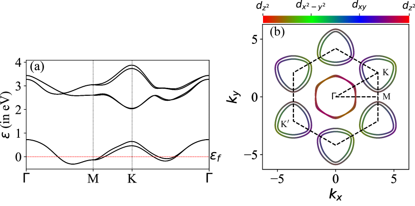
Figure 13: (a) The band structure with full bandwith. (b) The Fermi surface colored according to the orbital content.

Fig. 13-(a) shows Ising SOC spilt bands. There are total 6-bands. We primarily focus on low energy bands crossing the Fermi surface. Fig. 13-(b) shows orbital resolved Fermi surface. As can be seen in figure $\Gamma$-centered pocket is primarily dominated by $d_{z^{2}}$ orbital and the K-centered pockets are primarily dominated by degenerate $d_{x^{2}-y^{2}}$ and $d_{xy}$ orbitals.

Appendix B The effective pairing interaction

Here we give a detailed derivation of the pairing kernel used in the main paper, Eqn.(4). The rotationally invariant interaction Hamiltonian is given by

$$H_{\mathrm{int}} = \frac{U}{2}\sum_{i,\mu,\sigma}n_{i\mu\sigma}n_{i\mu\bar{\sigma}}+\frac{U^{\prime}}{2}\sum_{i,\mu\neq\nu,\sigma}n_{i\mu\sigma}n_{i\nu\bar{\sigma}}$$ (19)

$$+ \frac{U^{\prime}-J}{2}\sum_{i,\mu\neq\nu,\sigma}n_{i\mu\sigma}n_{i\nu\sigma}$$

$$+ \frac{J}{2}\sum_{i,\mu\neq\nu}\sum_{\sigma}\left[c^{+}_{i\mu\sigma}c^{+}_{i\nu\bar{\sigma}}c_{i\mu\bar{\sigma}}c_{i\nu\sigma}\right]$$

$$+ \frac{J^{\prime}}{2}\sum_{i,\mu\neq\nu}\sum_{\sigma}\left[c^{+}_{i\mu\sigma}c^{+}_{i\mu\bar{\sigma}}c_{i\nu\bar{\sigma}}c_{i\nu\sigma}\right]$$

Here, the $U$ term, the $U^{\prime}$ term, and the $J$ term denote the intra-orbital, inter-orbital Hubbard repulsion and the Hund’s rule coupling as well as the pair hopping. We work in the spin-rotational invariant setting where the onsite Coulomb terms are related by $U=U^{\prime}+2J$ and $J=J^{\prime}$. Restricting to Cooper pair channel the above interaction Hamiltonian can be re-written with a compact notation as following

$$H_{\mathrm{int}}=\frac{1}{2}\sum_{\mathbf{k},\mathbf{k}^{\prime},\tilde{l}}[U]^{\tilde{l}_{1},\tilde{l}_{2}}_{\tilde{l}_{3},\tilde{l}_{4}}\,c^{\dagger}_{\mathbf{k},\tilde{l}_{1}}\,c^{\dagger}_{-\mathbf{k},\tilde{l}_{3}}\,c_{-\mathbf{k}^{\prime},\tilde{l}_{2}}\,c_{\mathbf{k}^{\prime},\tilde{l}_{4}}$$ (20)

Figure 14: Effective pairinig vertex

Here, $[\tilde{l}:=(l,\sigma)]$. The bare electron-electron interaction $[U]^{\tilde{l}_{1},\tilde{l}_{2}}_{\tilde{l}_{3},\tilde{l}_{4}}$, i.e. the first order correction in $[V]^{\tilde{l}_{1},\tilde{l}_{2}}_{\tilde{l}_{3},\tilde{l}_{4}}$ is given by

$[U]_{\mu\bar{s}\mu s}^{\mu s\mu\bar{s}}=U$	$[U]_{\mu\bar{s}\nu s}^{\nu s\mu\bar{s}}=U^{\prime}$	$[U]_{\mu\bar{s}\nu s}^{\mu s\nu\bar{s}}=J^{\prime}$
$[U]_{\nu\bar{s}\nu s}^{\mu s\mu\bar{s}}=J$	$[U]_{\nu s\mu s}^{\mu s\nu s}=U^{\prime}-J$
$[U]_{\mu\bar{s}\mu\bar{s}}^{\mu s\mu s}=-U$	$[U]_{\mu\bar{s}\mu\bar{s}}^{\nu s\nu s}=-U^{\prime}$	$[U]_{\mu\bar{s}\nu\bar{s}}^{\mu s\nu s}=-J^{\prime}$
$[U]_{\nu\bar{s}\mu\bar{s}}^{\mu s\nu s}=-J$	$[U]_{\nu s\nu s}^{\mu s\mu s}=-U^{\prime}+J$

For higher order correction in $[V]^{\tilde{l}_{1},\tilde{l}_{2}}_{\tilde{l}_{3},\tilde{l}_{4}}$ we sum up all bubble and ladder diagrams to infinite order in $U$ (RPA).

B.1 Bubble Diagrams

Figure 15: Second order Bubble diagram

The second order bubble diagram shown in Fig. (15) can be written as

$$U^{\tilde{l}_{1},\tilde{\nu}_{2}}_{\tilde{\nu}_{1},\tilde{l}_{4}}\,\,\chi^{\tilde{\nu}_{1},\tilde{\nu}_{2}}_{\tilde{\nu}_{3},\tilde{\nu}_{4}}\,\,U^{\tilde{\nu}_{3},\tilde{l}_{2}}_{\tilde{l}_{3},\tilde{\nu}_{4}}$$ (21)

with anti-commutation properties of operators,

$$(-U^{\tilde{l}_{1},\tilde{l}_{4}}_{\tilde{\nu}_{1},\tilde{\nu}_{2}})\,\,\chi^{\tilde{\nu}_{1},\tilde{\nu}_{2}}_{\tilde{\nu}_{3},\tilde{\nu}_{4}}\,\,(-U^{\tilde{\nu}_{3},\tilde{\nu}_{4}}_{\tilde{l}_{3},\tilde{l}_{2}})$$ (22)

In language of matrices this is simply

$$[U\,\chi\,U]^{\tilde{l}_{1},\tilde{l}_{4}}_{\tilde{l}_{3},\tilde{l}_{2}}$$ (23)

Figure 16: Third order Bubble diagram

The third order bubble diagram shown in Fig. (16) is given as

$$(-U^{\tilde{l}_{1},\tilde{l}_{4}}_{\tilde{\nu}_{1},\tilde{\nu}_{2}})\,\,\chi^{\tilde{\nu}_{1},\tilde{\nu}_{2}}_{\tilde{\nu}_{3},\tilde{\nu}_{4}}\,\,(-U^{\tilde{\nu}_{3},\tilde{\nu}_{4}}_{\tilde{\nu}_{1}^{\prime},\tilde{\nu}_{2}^{\prime}})\,\,\chi^{\tilde{\nu}_{1}^{\prime},\tilde{\nu}_{2}^{\prime}}_{\tilde{\nu}_{3}^{\prime},\tilde{\nu}_{4}^{\prime}}\,\,(-U^{\tilde{\nu}_{3}^{\prime},\tilde{\nu}_{4}^{\prime}}_{\tilde{l}_{3},\tilde{l}_{2}}),$$ (24)

or un matrix notation

$$-[U\,\chi\,U\,\chi\,U]^{\tilde{l}_{1},\tilde{l}_{4}}_{\tilde{l}_{3},\tilde{l}_{2}}.$$ (25)

So, if we consider all orders of bubble diagrams, we get terms alternating in sign, a $n_{\text{th}}$ order term having the sign $(-1)^{n}$.
Thus the total contribution from all the bubble diagrams can be represented as following summation of all the orders in bubble

$$-[V^{\mathrm{{Total}}}_{\mathrm{bub}}]^{\tilde{l}_{1},\tilde{l}_{2}}_{\tilde{l}_{3},\tilde{l}_{4}} = \left[(-U)\,\chi\,(-U)\right]^{\tilde{l}_{1},\tilde{l}_{4}}_{\tilde{l}_{3},\tilde{l}_{2}}-\left[(-U)\,\chi\,(-U)\,\chi\,(-U)\right]^{\tilde{l}_{1},\tilde{l}_{4}}_{\tilde{l}_{3},\tilde{l}_{2}}+\left[(-U)\,\chi\,(-U)\,\chi\,(-U)\,\chi\,(-U)\right]^{\tilde{l}_{1},\tilde{l}_{4}}_{\tilde{l}_{3},\tilde{l}_{2}}-\ldots$$ (26)

$$= \left[\frac{(-U)\,\chi\,(-U)}{1+\chi\,(-U)}\right]^{\tilde{l}_{1},\tilde{l}_{4}}_{\tilde{l}_{3},\tilde{l}_{2}}$$

B.2 Ladder Diagrams

Lets, bring our attention to the ladders now

Figure 17: Second order Ladder diagram

Fig. (17) with anti-commutation property of operators can be written as

$$U^{\tilde{l}_{1},\tilde{l}_{2}}_{\tilde{\nu}_{1},\tilde{\nu}_{2}}\,\,\chi^{\tilde{\nu}_{1},\tilde{\nu}_{2}}_{\tilde{\nu}_{3},\tilde{\nu}_{4}}\,\,U^{\tilde{\nu}_{3},\tilde{\nu}_{4}}_{\tilde{l}_{3},\tilde{l}_{4}}=[U\,\chi\,U]^{\tilde{l}_{1},\tilde{l}_{2}}_{\tilde{l}_{3},\tilde{l}_{4}}$$ (27)

Figure 18: Third order Ladder diagram

For, the third order ladder diagram in Fig. (18) we have

$$U^{\tilde{l}_{1},\tilde{l}_{2}}_{\tilde{\nu_{1}},\tilde{\nu}_{2}}\,\,\chi^{\tilde{\nu}_{1},\tilde{\nu}_{2}}_{\tilde{\nu}_{2}^{\prime},\tilde{\nu}_{1}^{\prime}}\,\,U^{\tilde{\nu}_{2}^{\prime},\tilde{\nu}_{1}^{\prime}}_{\tilde{\nu}_{4}^{\prime},\tilde{\nu}_{3}^{\prime}}\,\,\chi^{\tilde{\nu}_{4}^{\prime},\tilde{\nu}_{3}^{\prime}}_{\tilde{\nu}_{3},\tilde{\nu}_{4}}\,\,U^{\tilde{\nu}_{3}^{\prime},\tilde{\nu}_{4}}_{\tilde{l}_{3},\tilde{l}_{4}}=[U\,\chi\,U\,\chi\,U]^{\tilde{l}_{1},\tilde{l}_{2}}_{\tilde{l}_{3},\tilde{l}_{4}}$$ (28)

Like bubble diagrams we will be doing summation in all orders of ladder diagrams. Few things to note here which is different in summation of ladder diagrams than summation in bubble diagrams As there is no fermionic looping, the susceptibility expression appears with a “$-$” sign in front.There is no alternating signs appearing in series of ladder diagrams so, the denominator appears with a ”$-$” sign.

$$-[V^{\mathrm{{Total}}}_{\mathrm{ladder}}]^{\tilde{l}_{1},\tilde{l}_{2}}_{\tilde{l}_{3},\tilde{l}_{4}} = \left[(-U)\,(-\chi)\,(-U)\right]^{\tilde{l}_{1},\tilde{l}_{4}}_{\tilde{l}_{3},\tilde{l}_{2}}+\left[(-U)\,(-\chi)\,(-U)\,(-\chi)\,(-U)\right]^{\tilde{l}_{1},\tilde{l}_{4}}_{\tilde{l}_{3},\tilde{l}_{2}}$$ (29)

$$+ \left[(-U)\,(-\chi)\,(-U)\,(-\chi)\,(-U)\,(-\chi)\,(-U)\right]^{\tilde{l}_{1},\tilde{l}_{4}}_{\tilde{l}_{3},\tilde{l}_{2}}\ldots$$

$$= \left[\frac{(-U)\,(-\chi)\,(-U)}{1-(-\chi)\,(-U)}\right]^{\tilde{l}_{1},\tilde{l}_{4}}_{\tilde{l}_{3},\tilde{l}_{2}}$$

From the preceding discussion, in presence of spin orbit coupling the final interaction vertex can be written as

$$[V(\mathbf{k},\mathbf{k}^{\prime})]^{\tilde{l}_{1},\tilde{l}_{2}}_{\tilde{l}_{3},\tilde{l}_{4}} = [U]^{\tilde{l}_{1},\tilde{l}_{2}}_{\tilde{l}_{3},\tilde{l}_{4}}-[\frac{U\,\chi_{0}\,U}{1-\chi_{0}\,U}]^{\tilde{l}_{1},\tilde{l}_{4}}_{\tilde{l}_{3},\tilde{l}_{2}}(\mathbf{k}-\mathbf{k}^{\prime})+[\frac{U\,\chi_{0}\,U}{1-\chi_{0}\,U}]^{\tilde{l}_{1},\tilde{l}_{2}}_{\tilde{l}_{3},\tilde{l}_{4}}(\mathbf{k}+\mathbf{k}^{\prime})$$ (30)

Appendix C Gap equation for multibband superconductors

C.1 In absence of magnetic field

In the following we derive the Gorkov equations and superconducting gap equation for a generic multi band Hamiltonian. Assuming a homogeneous superconducting state, the Hamiltonian for a multi band superconductor can be expressed as,

$$H = H_{0}+H_{\mathrm{sc}}$$ (31)

$$H_{0} = \sum_{\mathbf{k}n\sigma}\epsilon_{n\sigma}(\mathbf{k})a^{{\dagger}}_{\mathbf{k}n\sigma}a_{\mathbf{k}n\sigma}$$ (32)

$$H_{\mathrm{sc}} = \frac{1}{2}\sum_{n_{i}\sigma_{i}\mathbf{k}\mathbf{k}^{\prime}}V_{n\sigma}(\mathbf{k},\mathbf{k}^{\prime})a^{{\dagger}}_{-\mathbf{k}n_{1}\sigma_{1}}a^{{\dagger}}_{\mathbf{k}n_{2}\sigma_{2}}a_{\mathbf{k}^{\prime}n_{3}\sigma_{3}}a_{-\mathbf{k}^{\prime}n_{4}\sigma_{4}}$$ (33)

With, $[V]^{\tilde{\mu_{1}},\tilde{\mu_{2}}}_{\tilde{\mu_{3}},\tilde{\mu_{4}}}$ the above Hamiltonian is written in a multi band basis where $a_{\mathbf{k}n\sigma}$($a_{\mathbf{k}n\sigma}^{\dagger}$) annihilates (creates) an electron in band $n$, at momenta $\mathbf{k}$, and quantum number $\sigma$. If the non interacting Hamiltonian preserves the $S_{z}$ quantum number then we can identify $\sigma$ with the true spin, $\sigma=(\uparrow,\downarrow)$. This would be true for example either in the absence of a spin orbit coupling or presence of a spin orbit coupling that does not generate off diagonal matrix elements (spin flip contributions). In the presence of spin flip contributions $\sigma$ would represent a pseudo spin index.

(For ease of notation we have changed the convention of writing down the pair potential, $[V]^{\tilde{\mu_{1}},\tilde{\mu_{2}}}_{\tilde{\mu_{3}},\tilde{\mu_{4}}}$ in equation 33 is same as $[V]^{\tilde{\mu_{3}},\tilde{\mu_{1}}}_{\tilde{\mu_{4}},\tilde{\mu_{2}}}$ in equation 20.)

In the following calculation we will be studying the above Hamiltonian without assuming any specific form of non interacting Hamiltonian.
Let us define the generic Green’s functions relevant to the problem as,

$$G^{\sigma,\sigma^{\prime}}_{n,n^{\prime}}(\mathbf{k},\tau_{1};\mathbf{k}^{\prime},\tau_{2}) = -\bigl{\langle}T_{\tau}a_{\mathbf{k},n,\sigma}(\tau_{1})a^{\dagger}_{\mathbf{k}^{\prime},n^{\prime},\sigma^{\prime}}(\tau_{2})\bigr{\rangle}$$ (34)

$$F^{\sigma,\sigma^{\prime}}_{n,n^{\prime}}(\mathbf{k},\tau_{1};\mathbf{k}^{\prime},\tau_{2}) = \bigl{\langle}T_{\tau}a_{\mathbf{k},n,\sigma}(\tau_{1})a_{-\mathbf{k}^{\prime},n^{\prime},\sigma^{\prime}}(\tau_{2})\bigr{\rangle}$$ (35)

$$F^{*\sigma,\sigma^{\prime}}_{n,n^{\prime}}(\mathbf{k},\tau_{1};\mathbf{k}^{\prime},\tau_{2}) = \bigl{\langle}T_{\tau}a^{\dagger}_{-\mathbf{k},n,\sigma}(\tau_{1})a^{\dagger}_{\mathbf{k}^{\prime},n^{\prime},\sigma^{\prime}}(\tau_{2})\bigr{\rangle}$$ (36)

Here $T_{\tau}$ is the time time ordering operator in the imaginary time ($\tau$) formalism. After a mean field decomposition, the superconducting gap equation can be defined as,

$$\Delta^{n_{2},n_{1}}_{\sigma_{2},\sigma_{1}}(\mathbf{k}) = -\sum_{\mathbf{k}^{\prime},n_{3},n_{4},\sigma_{3},\sigma_{4}}V^{n_{1},n_{2},\sigma_{1},\sigma_{2}}_{n_{3},n_{4},\sigma_{3},\sigma_{4}}(\mathbf{k},\mathbf{k}^{\prime})\bigl{\langle}a_{\mathbf{k}^{\prime},n_{3},\sigma_{3}}(\tau)a_{-\mathbf{k}^{\prime},n_{4},\sigma_{4}}(\tau)\bigr{\rangle}$$ (37)

$$\Delta^{\ast n_{2},n_{1}}_{\sigma_{2},\sigma_{1}}(\mathbf{k}) = -\sum_{\mathbf{k}^{\prime},n_{3},n_{4},\sigma_{3},\sigma_{4}}V^{n_{1},n_{2},\sigma_{1},\sigma_{2}}_{n_{3},n_{4},\sigma_{3},\sigma_{4}}(\mathbf{k}^{\prime},\mathbf{k})\bigl{\langle}a^{\dagger}_{-\mathbf{k}^{\prime},n_{3},\sigma_{3}}(\tau)a^{\dagger}_{\mathbf{k}^{\prime},n_{4},\sigma_{4}}(\tau)\bigr{\rangle}$$ (38)

In the above the we do not assume a particular mechanism for the origin of superconducting pairing potential. The pair potential can be considered to be given by matrix elements given by,

$$V^{n_{1},n_{2},\sigma_{1},\sigma_{2}}_{n_{3},n_{4},\sigma_{3},\sigma_{4}}(\mathbf{k},\mathbf{k}^{\prime})=\bigl{\langle}-\mathbf{k},n_{1},\sigma_{1};\mathbf{k},n_{2},\sigma_{2}\bigl{|}\hat{V}\bigr{|}-\mathbf{k}^{\prime},n_{4},\sigma_{4};\mathbf{k}^{\prime},n_{3},\sigma_{3}\bigr{\rangle}$$ (39)

Equation 39 has the following symmetry properties

$$\left.\begin{aligned} V^{n_{1},n_{2},\sigma_{1},\sigma_{2}}_{n_{3},n_{4},\sigma_{3},\sigma_{4}}(\mathbf{k},\mathbf{k}^{\prime})=V^{n_{2},n_{1},\sigma_{2},\sigma_{1}}_{n_{4},n_{3},\sigma_{4},\sigma_{3}}(-\mathbf{k},-\mathbf{k}^{\prime})=V^{n_{2},n_{1},\sigma_{2},\sigma_{1}}_{n_{3},n_{4},\sigma_{3},\sigma_{4}}(-\mathbf{k},\mathbf{k}^{\prime})=V^{n_{1},n_{2},\sigma_{1},\sigma_{2}}_{n_{4},n_{3},\sigma_{4},\sigma_{3}}(\mathbf{k},-\mathbf{k}^{\prime})=V^{n_{4},n_{3},\sigma_{4},\sigma_{3}}_{n_{2},n_{1},\sigma_{2},\sigma_{1}}(\mathbf{k}^{\prime},\mathbf{k})\end{aligned}\right\}$$ (40)

In the following we use the equation of motion for the Greens functions to derive the Gorkov equation’s, and the following anti-commutation property of the operators,

$$\left[\hat{A}\hat{B},\hat{C}\right] = \hat{A}\{\hat{B},\hat{C}\}-\{\hat{A},\hat{C}\}\hat{B}$$ (41)

$$\left[\hat{A}\hat{B}\hat{C}\hat{D},\hat{E}\right] = \hat{A}\hat{B}[\hat{C}\hat{D},\hat{E}]+[\hat{A}\hat{B},\hat{E}]\hat{C}\hat{D}$$ (42)

$$\left[\hat{A}\hat{B}\hat{C}\hat{D},\hat{E}\right] = \hat{A}\hat{B}\hat{C}\{\hat{D},\hat{E}\}-\hat{A}\hat{B}\{\hat{C},\hat{E}\}\hat{D}+\hat{A}\{\hat{B},\hat{E}\}\hat{C}\hat{D}-\{\hat{A},\hat{E}\}\hat{B}\hat{C}\hat{D}$$ (43)

For the particle hole Greens’ function we get (using Eq. (34))

$$\frac{\partial G^{\sigma,\sigma^{\prime}}_{n,n^{\prime}}}{\partial\tau}=-\frac{\partial\bigl{\langle}T_{\tau}a_{\mathbf{k},n,\sigma}(\tau)a^{\dagger}_{\mathbf{k}^{\prime},n^{\prime},\sigma^{\prime}}(0)\bigr{\rangle}}{\partial\tau}=-\delta(\tau)\delta_{n,n^{\prime}}\delta_{\mathbf{k},\mathbf{k}^{\prime}}\delta_{\sigma,\sigma^{\prime}}-\bigl{\langle}T_{\tau}\left[H,a_{\mathbf{k},n,\sigma}(\tau)\right]a^{\dagger}_{\mathbf{k}^{\prime},n^{\prime},\sigma^{\prime}}(0)\bigr{\rangle}$$ (44)

The commutator with the Hamiltonian involves $\left[H_{0}(\tau)+H_{\mathrm{sc}}(\tau),a_{\mathbf{k},n,\sigma}(\tau)\right]$. Using Eq. (32) we obtain

$$\left[H_{0}(\tau),a_{\mathbf{k},n,\sigma}(\tau)\right] = -\epsilon_{n\sigma}(\mathbf{k})a_{\mathbf{k}n\sigma}(\tau).$$ (45)

In the above we utilize the anti commutation relationships between the Fermion operators. Similarly, from Eq 33

$$\left[H_{\mathrm{sc}},a_{\mathbf{k},\tilde{m}}(\tau)\right] = \sum_{\tilde{m}_{i},\textbf{s}}V^{\tilde{m}_{1},\tilde{m}}_{\tilde{m}_{3},\tilde{m}_{4}}(\mathbf{k},\textbf{s})a^{{\dagger}}_{-\mathbf{k}\tilde{m}_{1}}(\tau)a_{\textbf{s}\tilde{m}_{3}}(\tau)a_{-\textbf{s}\tilde{m}_{4}}(\tau)$$ (46)

Note that in the above equation we have introduced a compact notation $\tilde{m}_{i}=(n_{i},\sigma_{i})$. Replacing the results from Eq 45, and Eq 46 into Eq 44 we get

$$\frac{\partial G_{\tilde{m},\tilde{m}^{\prime}}}{\partial\tau} = -\delta(\tau)\delta_{\tilde{m},\tilde{m}^{\prime}}\delta_{\mathbf{k},\mathbf{k}^{\prime}}+\epsilon_{\tilde{m}}(\mathbf{k})\bigl{\langle}T_{\tau}a_{\mathbf{k}\tilde{m}}(\tau)a^{\dagger}_{\mathbf{k}^{\prime}\tilde{m}^{\prime}}(0)\bigr{\rangle}$$ (47)

$$-\sum_{\begin{subarray}{c}\tilde{m}_{1}\rightarrow\tilde{m}_{3}\\ \mathbf{p}\end{subarray}}V^{\tilde{m}_{1},\tilde{m}}_{\tilde{m}_{2},\tilde{m}_{3}}(\mathbf{k},\mathbf{p})\bigl{\langle}T_{\tau}a^{{\dagger}}_{-\mathbf{k}\tilde{m}_{1}}(\tau)a_{\mathbf{p}\tilde{m}_{2}}(\tau)a_{-\mathbf{p}\tilde{m}_{3}}(\tau)a^{\dagger}_{\mathbf{k}^{\prime}\tilde{m}^{\prime}}(0)\bigr{\rangle}$$

Now performing mean field decomposition

$$\frac{\partial G_{\tilde{m},\tilde{m}^{\prime}}}{\partial\tau}(\mathbf{k},\tau;\mathbf{k}^{\prime},0)=-\delta(\tau)\delta_{\tilde{m},\tilde{m}^{\prime}}\delta_{\mathbf{k},\mathbf{k}^{\prime}}-\epsilon_{\tilde{m}}(\mathbf{k})G_{\tilde{m},\tilde{m}^{\prime}}(\mathbf{k},\tau;\mathbf{k}^{\prime},0)+\sum_{\tilde{m}_{1}}\Delta^{\tilde{m},\tilde{m}_{1}}(\mathbf{k})F^{\ast}_{\tilde{m}_{1},\tilde{m}^{\prime}}(\mathbf{k},\tau;\mathbf{k}^{\prime},0)$$ (48)

Here, $\Delta^{\tilde{m},\tilde{m}_{1}}(\mathbf{k})=-\sum_{\mathbf{p},\tilde{m}_{2},\tilde{m}_{3}}V^{\tilde{m}_{1},\tilde{m}}_{\tilde{m}_{2},\tilde{m}_{3}}(\mathbf{k},\mathbf{p})\bigl{\langle}a_{\mathbf{p},\tilde{m}_{2}}(\tau)a_{-\mathbf{p},\tilde{m}_{3}(\tau)}\bigr{\rangle}$. We can do the same procedure for $F$ and $F^{\ast}$ and use the transformation to Matsubara frequencies $G_{\tilde{m},\tilde{m}^{\prime}}(\mathbf{k},\tau;\mathbf{k}^{\prime},0)=k_{\mathrm{B}}T\sum_{n}G_{\tilde{m},\tilde{m}^{\prime}}(\mathbf{k},\mathbf{k}^{\prime};\omega_{n})\exp{(-i\,\omega_{n}\tau)}$, this leads to following Gorkov equations

$$(i\omega_{n}-\epsilon_{\tilde{m}}(\mathbf{k}))G^{\tilde{m},\tilde{m}^{\prime}}(\mathbf{k},\mathbf{k}^{\prime};\omega_{n})+\sum_{\tilde{m}_{1}}\Delta^{\tilde{m},\tilde{m}_{1}}(\mathbf{k})F^{\ast\tilde{m}_{1},\tilde{m}^{\prime}}(\mathbf{k},\mathbf{k}^{\prime};\omega_{n}) = \delta_{\mathbf{k},\mathbf{k}^{\prime}}\delta_{\tilde{m},\tilde{m}^{\prime}}$$ (49)

$$(i\omega_{n}-\epsilon_{\tilde{m},\sigma}(\mathbf{k}))F^{\tilde{m},\tilde{m}^{\prime}}(\mathbf{k},\mathbf{k}^{\prime};\omega_{n})-\sum_{\tilde{m}_{1}}\Delta^{\tilde{m},\tilde{m}_{1}}(\mathbf{k})G^{\tilde{m}^{\prime},\tilde{m}_{1}}(-\mathbf{k}^{\prime},-\mathbf{k};-\omega_{n}) = 0$$ (50)

$$(i\omega_{n}+\epsilon_{m}(-\mathbf{k}))F^{\ast m,m^{\prime}}(\mathbf{k},\mathbf{k}^{\prime};\omega_{n})+\sum_{m_{1}}\Delta^{\ast m_{1},m}(\mathbf{k})G^{m_{1},m^{\prime}}(\mathbf{k},\mathbf{k}^{\prime};\omega_{n}) = 0$$ (51)

Then for translationally invariant system $G^{m,m^{\prime}}(\mathbf{k},\mathbf{k}^{\prime};\omega_{n})=G^{m,m^{\prime}}(\mathbf{k},\omega_{n})\delta(\mathbf{k}-\mathbf{k}^{\prime})$.

The Gorkov equations reduce to

$$(i\omega_{n}-\epsilon_{\tilde{m}}(\mathbf{k}))G^{\tilde{m},\tilde{m}^{\prime}}(\mathbf{k},\omega_{n})+\sum_{m_{1}}\Delta^{\tilde{m},\tilde{m}_{1}}(\mathbf{k})F^{\ast\tilde{m}_{1},\tilde{m}^{\prime}}(\mathbf{k},\omega_{n}) = \delta_{m,m^{\prime}}$$ (52)

$$(i\omega_{n}-\epsilon_{m}(\mathbf{k}))F^{\tilde{m},\tilde{m}^{\prime}}(\mathbf{k},\omega_{n})-\sum_{m_{1}}\Delta^{\tilde{m},\tilde{m}_{1}}(\mathbf{k})G^{\tilde{m}^{\prime},\tilde{m}_{1}}(-\mathbf{k},-\omega_{n}) = 0$$ (53)

$$(i\omega_{n}+\epsilon_{m}(-\mathbf{k}))F^{\ast\tilde{m},\tilde{m}^{\prime}}(\mathbf{k},\omega_{n})+\sum_{\tilde{m}_{1}}\Delta^{\ast\tilde{m}_{1},\tilde{m}}(\mathbf{k})G^{\tilde{m}_{1},\tilde{m}^{\prime}}(\mathbf{k},\omega_{n}) = 0,$$ (54)

where

$$\Delta^{\tilde{m}_{2},\tilde{m}_{1}}(\mathbf{k}) = -\sum_{\begin{subarray}{c}n,\tilde{m}_{3},\tilde{m}_{4},\\ \mathbf{k}\end{subarray}}V^{\tilde{m}_{1},\tilde{m}_{2}}_{\tilde{m}_{3},\tilde{m}_{4}}(\mathbf{k},\mathbf{k}^{\prime})F^{\tilde{m}_{3},\tilde{m}_{4}}(\mathbf{k}^{\prime},\omega_{n}).$$ (55)

To evaluate the linearized gap equation we consider F to be linear order in $\Delta$. This is achieved by replacing $G\rightarrow G^{0}$.
Then from Eq. (53) we get

$$F^{\tilde{m},\tilde{m}^{\prime}}(\mathbf{k},\omega_{n})=\sum_{\tilde{m}_{1}}\frac{\Delta^{\tilde{m},\tilde{m}_{1}}(\mathbf{k})G^{(0)\tilde{m}^{\prime},\tilde{m}_{1}}(-\mathbf{k},-\omega_{n})}{(i\omega_{n}-\epsilon_{\tilde{m}}(\mathbf{k}))}$$ (56)

and from Eq. (52)

$$G^{(0)\tilde{m}^{\prime},\tilde{m}_{1}}(-\mathbf{k},-\omega_{n})=-\frac{\delta_{\tilde{m}^{\prime},\tilde{m}_{1}}}{(i\omega_{n}+\epsilon_{\tilde{m}^{\prime}}(-\mathbf{k}))}$$ (57)

Combining the previous two equations we get

$$F^{\tilde{m},\tilde{m}^{\prime}}(\mathbf{k},\omega_{n}) = -\sum_{\tilde{m}_{1}}\frac{\Delta^{\tilde{m},\tilde{m}_{1}}(\mathbf{k})\delta_{\tilde{m}^{\prime},\tilde{m}_{1}}}{(i\omega_{n}-\epsilon_{\tilde{m}}(\mathbf{k}))(i\omega_{n}+\epsilon_{\tilde{m}^{\prime}}(-\mathbf{k}))}$$ (58)

$$= -\frac{\Delta^{\tilde{m},\tilde{m}^{\prime}}(\mathbf{k})}{(i\omega_{n}-\epsilon_{\tilde{m}}(\mathbf{k}))(i\omega_{n}+\epsilon_{\tilde{m}^{\prime}}(-\mathbf{k}))}$$

Putting the previous equation back to 55 we get the linearized gap equation for a generic multi band homogeneous system

$$\Delta^{\tilde{m}_{1},\tilde{m}_{2}}(\mathbf{k}) = \sum_{\begin{subarray}{c}n,\tilde{m}_{3},\tilde{m}_{4},\\ \mathbf{k}^{\prime}\end{subarray}}\frac{V^{\tilde{m}_{2},\tilde{m}_{1}}_{\tilde{m}_{3},\tilde{m}_{4}}(\mathbf{k},\mathbf{k}^{\prime})\Delta^{\tilde{m}_{3},\tilde{m}_{4}}(\mathbf{k}^{\prime})}{(i\omega_{n}-\epsilon_{\tilde{m}_{3}}(\mathbf{k}^{\prime}))(i\omega_{n}+\epsilon_{\tilde{m}_{4}}(-\mathbf{k}^{\prime}))}$$ (59)

For system with Ising SOC Let us assume the $(\mathbf{k},\mathbf{k}^{\prime})$ represent the wave vectors for two bands that form the Fermi surface in the presence of Ising spin orbit coupling. Then we have in Eq 59

$$\left.\begin{aligned} \tilde{m}_{1}\neq\tilde{m}_{2}\\ \tilde{m}_{3}\neq\tilde{m}_{4}\end{aligned}\right\}$$ (60)

$$\epsilon_{\tilde{m}_{3}}(\mathbf{k}^{\prime})=\epsilon_{\tilde{m}_{4}}(-\mathbf{k}^{\prime})$$ (61)

and Eq. (59) can be rewritten as

$$\Delta^{\tilde{m}_{1},\tilde{m}_{2}}(\mathbf{k}) = -\sum_{\begin{subarray}{c}n,\tilde{m}_{3},\tilde{m}_{4},\\ \mathbf{k}^{\prime}\end{subarray}}\frac{V^{\tilde{m}_{2},\tilde{m}_{1}}_{\tilde{m}_{3},\tilde{m}_{4}}(\mathbf{k},\mathbf{k}^{\prime})\Delta^{\tilde{m}_{3},\tilde{m}_{4}}(\mathbf{k}^{\prime})}{\omega^{2}_{n}+\epsilon^{2}_{\tilde{m}_{3}}(\mathbf{k}^{\prime})}.$$ (62)

The definition for gap function should have an extra $k_{\mathrm{B}}T$ factor that we ignore here (this factor cancels with a similar term from the Fourier transform of the Greens function so the form of gap function is not affected).

For the two band´ system considered here, the wave vectors take two sets of values for $\tilde{m}=(n,\sigma)$. These are $\tilde{m}=(1,\uparrow)$ for set of points $\mathbf{k}_{1}$ on band 1 and $\tilde{m}=(2,\downarrow)$ for set of points $\mathbf{k}_{2}$ on band 2. Note that for a given wavevector $\mathbf{k}_{1}$ on band 1, we must have $-\mathbf{k}_{1}$ lying on band 2 (i.e the vector $-\mathbf{k}_{1}$ lies within the set of points $\mathbf{k}_{2}$). From equation 59 we split the momentum sum into sum over band 1 and band 2.

$$\Delta^{1,2}_{\uparrow\downarrow}(\mathbf{k}_{1}) = -\sum_{n\mathbf{k}^{\prime}_{{1}}}\frac{V^{2,1,\downarrow,\uparrow}_{1,2,\uparrow,\downarrow}(\mathbf{k}_{{1}},\mathbf{k}_{{1}}^{\prime})\Delta^{1,2}_{\uparrow\downarrow}(\mathbf{k}_{{1}}^{\prime})}{\omega^{2}_{n}+\epsilon^{2}_{1\uparrow}(\mathbf{k}_{{1}}^{\prime})}-\sum_{n\mathbf{k}^{\prime}_{{2}}}\frac{V^{2,1,\downarrow,\uparrow}_{2,1,\downarrow,\uparrow}(\mathbf{k}_{1},\mathbf{k}_{{2}}^{\prime})\Delta^{2,1}_{\downarrow\uparrow}(\mathbf{k}_{{2}}^{\prime})}{\omega^{2}_{n}+\epsilon^{2}_{2\downarrow}(\mathbf{k}_{{2}}^{\prime})}$$ (63)

A similar equation is obtained for $\Delta^{2,1}_{\downarrow\uparrow}(\mathbf{k}_{2})$. Note that the above equation considers zero momentum and zero frequency pairings only. Since the above equation explicitly incorporates the band index, it includes the points of degeneracy where the Ising spin orbit coupling vanishes leading to $\epsilon_{1\uparrow}(\mathbf{k})=\epsilon_{2\downarrow}(\mathbf{k})$.

As a next step, we perform the Matsubara sum and use the BCS approximation to restrict the pairing Kernel to a thin shell over the Fermi surface. Converting $\sum_{\mathbf{k}_{i}}f(\mathbf{k}_{i})\rightarrow\int d\epsilon_{i}\langle f(\mathbf{k}_{i})\rangle_{\mathbf{k}_{i}=\mathbf{k}_{Fi}}$, performing the energy integral, we can express the coupled equations in a matrix form as,

$$\begin{pmatrix}\Delta^{1,2}_{\uparrow,\downarrow}(\mathbf{k}_{F_{1}})\\ \Delta^{2,1}_{\downarrow,\uparrow}(\mathbf{k}_{F_{2}})\end{pmatrix}=-\ln\left(\frac{2\omega_{c}e^{\gamma}}{\pi k_{\mathrm{B}}T_{c}}\right)\begin{pmatrix}\frac{V^{2,1,\downarrow,\uparrow}_{1,2,\uparrow,\downarrow}(\mathbf{k}_{F_{1}},\mathbf{k}_{F_{1}}^{\prime})}{|\nabla\epsilon_{1,\uparrow}|_{\mathbf{k}^{\prime}=\mathbf{k}_{F_{1}}^{\prime}}}&\frac{V^{2,1,\downarrow,\uparrow}_{2,1,\downarrow,\uparrow}(\mathbf{k}_{F_{1}},\mathbf{k}_{F_{2}}^{\prime})}{|\nabla\epsilon_{2,\downarrow}|_{\mathbf{k}^{\prime}=\mathbf{k}_{F_{2}}^{\prime}}}\\ \frac{V^{1,2,\uparrow,\downarrow}_{1,2,\uparrow,\downarrow}(\mathbf{k}_{F_{2}},\mathbf{k}_{F_{1}}^{\prime})}{|\nabla\epsilon_{1,\uparrow}|_{\mathbf{k}^{\prime}=\mathbf{k}_{F_{1}}^{\prime}}}&\frac{V^{1,2,\uparrow,\downarrow}_{2,1,\downarrow,\uparrow}(\mathbf{k}_{F_{2}},\mathbf{k}_{F_{2}}^{\prime})}{|\nabla\epsilon_{2,\downarrow}|_{\mathbf{k}^{\prime}=\mathbf{k}_{F_{2}}^{\prime}}}\end{pmatrix}\begin{pmatrix}\Delta^{1,2}_{\uparrow,\downarrow}(\mathbf{k}_{F_{1}}^{\prime})\\ \Delta^{2,1}_{\downarrow,\uparrow}(\mathbf{k}_{F_{2}}^{\prime}),\end{pmatrix}$$ (64)

where $\omega_{c}$ is some cutoff that we assume to be the same for both band integrals. Note that for N $\mathbf{k}_{F_{1}}$ points, and N $\mathbf{k}_{F_{2}}$ points, the dimension of the gap equation matrix is $2N\times 2N$. The above linearized superconducting gap equation can be solved to determine the ground state gap solution. If the set of points on the band 1 Fermi surface are $\mathbf{k}_{F_{1}}=(\mathbf{k}_{1F_{1}},\mathbf{k}_{2F_{1}},\mathbf{k}_{3F_{1}},\mathbf{k}_{4F_{1}}\cdot\cdot\cdot\text{N points})$, and the N points on band 2 are ordered as $\mathbf{k}_{F_{2}}=(-\mathbf{k}_{1F_{1}},-\mathbf{k}_{2F_{1}},-\mathbf{k}_{3F_{1}},-\mathbf{k}_{4F_{1}}\cdot\cdot\cdot\text{N points})$ then using Eq 40, the off diagonal blocks of the gap equation matrix have the symmetry $V^{1,2,\uparrow,\downarrow}_{2,1,\downarrow,\uparrow}(\mathbf{k}_{F_{1}},\mathbf{k}_{F_{2}}^{\prime})=V^{2,1,\downarrow,\uparrow}_{1,2,\uparrow,\downarrow}(-\mathbf{k}_{F_{1}},-\mathbf{k}_{F_{2}}^{\prime})=V^{2,1,\downarrow,\uparrow}_{1,2,\uparrow,\downarrow}(\mathbf{k}_{F_{2}},\mathbf{k}_{F_{1}}^{\prime})$. Similarly the function $A_{\tilde{m}}(\mathbf{k})=1/|\nabla\epsilon_{\tilde{m}}(\mathbf{k})|$ on the two bands are related by $A_{1,\uparrow}(\mathbf{k}_{1})=A_{2,\downarrow}(-\mathbf{k}_{1})$

C.2 In Presence of Out of Plane Magnetic Field

In the following we study the effect of a longitudinal magnetic field to the monolayer NbSe₂. Although near the transition temperature the orbital effect (vector potential contribution) dominates, in this section we ignore the orbital effect and consider only the Pauli paramagnetism contribution within the superconducting state. In the orbital basis, the Zeeman field Hamiltonian will be given by

$$H_{B_{z}}=g\mu_{B}B_{z}\sum_{l,\mathbf{k}}(n_{\mathbf{k}l\uparrow}-n_{\mathbf{k}l\downarrow}),$$ (65)

where $n_{\mathbf{k}l\sigma}=c^{{\dagger}}_{\mathbf{k}l\sigma}c_{\mathbf{k}l\sigma}$. Assuming the non interacting Hamiltonian has no spin flip contribution, the above term keeps $S_{z}$ as a good quantum number. If we diagonalise the total Hamiltonian with the Zeeman term included, we can look at a model that considers the modification to the pairing term due to the magnetic field using a similar approach to the zero field case discussed above. We will only need to modify the gap equation in Eq 59. As discussed above the gap equation is a coupled set of equations

$$\Delta^{\tilde{m}_{1},\tilde{m}_{2}}(\mathbf{k}) = \sum_{\begin{subarray}{c}n,\tilde{m}_{3},\tilde{m}_{4},\\ \mathbf{k}^{\prime}\end{subarray}}\frac{V^{\tilde{m}_{2},\tilde{m}_{1}}_{\tilde{m}_{3},\tilde{m}_{4}}(\mathbf{k},\mathbf{k}^{\prime},B_{z})\Delta^{\tilde{m}_{3},\tilde{m}_{4}}(\mathbf{k}^{\prime})}{(i\omega_{n}-\epsilon_{\tilde{m}_{3}}(\mathbf{k}^{\prime}))(i\omega_{n}+\epsilon_{\tilde{m}_{4}}(-\mathbf{k}^{\prime}))}$$ (66)

Here, the magnetic field dependence enters both the pairing interaction and the single particle energies. By breaking the Kramers degeneracy the modified relation between the single particle energy on the two bands relevant to monolayer NbSe₂ read $\epsilon_{m_{3}/m_{4}}\rightarrow\epsilon_{m_{3}/m_{4}}\pm g\mu_{B}B_{z}$ since the indices $m_{3}$ and $m_{4}$ on the Fermi surface necessarily belong to the spin up and spin down bands or vice versa. This is also true for the Hamiltonian that ignores the spin orbit contribution when restricted to only opposite spin pairing singlet or triplet solutions. This implies the gap equation modifies to

$$\Delta^{\tilde{m}_{1},\tilde{m}_{2}}(\mathbf{k})=-\sum_{\begin{subarray}{c}n,\tilde{m}_{3},\tilde{m}_{4},\\ \mathbf{k}^{\prime}\end{subarray}}\frac{V^{\tilde{m}_{2},\tilde{m}_{1}}_{\tilde{m}_{3},\tilde{m}_{4}}(\mathbf{k},\mathbf{k}^{\prime},B_{z})\Delta^{\tilde{m}_{3},\tilde{m}_{4}}(\mathbf{k}^{\prime})}{\tilde{\omega}_{n}^{2}+\epsilon^{2}_{\tilde{m}_{3}}(\mathbf{k}^{\prime})}$$ (67)

where the Matsubara frequency is shifted by the field, $\tilde{\omega}_{n}=\omega_{n}\pm ig\mu_{B}B$, and the sign $\pm$ corresponding to $(\tilde{m}_{3},\tilde{m}_{4})=(2\downarrow,1\uparrow)$ or $(\tilde{m}_{4},\tilde{m}_{3})=(1\uparrow,2\downarrow)$ respectively. Note that the symmetry $\epsilon^{2}_{\tilde{m}_{3}}(\mathbf{k}^{\prime})=\epsilon_{\tilde{m}_{4}}(-\mathbf{k}^{\prime})$, is generically true for Ising SOC on any constant energy surface. For no spin orbit coupling we have the additional criterion $\tilde{m}_{1}=\tilde{m}_{2}$, and $\tilde{m}_{3}=\tilde{m}_{4}$ if we assume zero energy and zero momentum pairing.

For weak magnetic fields, we can consider the magnetic field to be a perturbation to the non interacting Hamiltonian. In this limit, we consider the Fermi surface to be the one obtained in zero magnetic field. Note that this Zeeman term that acts as a perturbation, will still make the energy integral and correspondingly the transition temperature field dependant but may not modify the gap matrix. It is interesting to ask how this formalism would differentiate between the even and odd parity superconducting states. Let us re-write the gap equation relevant to monolayer NbSe₂ in the presence of Ising SOC.

$$\Delta^{1,2}(\mathbf{k}_{1})=-\sum_{\begin{subarray}{c}n,\mathbf{k}^{\prime}_{1}\end{subarray}}\frac{V^{2,1}_{1,2}(\mathbf{k}_{1},\mathbf{k}^{\prime}_{1})\Delta^{1,2}(\mathbf{k}^{\prime}_{1})}{\tilde{\omega}_{n+}^{2}+\epsilon^{2}_{1}(\mathbf{k}^{\prime}_{1})}-\sum_{\begin{subarray}{c}n,\mathbf{k}^{\prime}_{2}\end{subarray}}\frac{V^{2,1}_{2,1}(\mathbf{k}_{2},\mathbf{k}^{\prime}_{2})\Delta^{2,1}(\mathbf{k}^{\prime}_{2})}{\tilde{\omega}_{n-}^{2}+\epsilon^{2}_{2}(\mathbf{k}^{\prime}_{2})}$$ (68)

$$\Delta^{2,1}(\mathbf{k}_{2})=-\sum_{\begin{subarray}{c}n,\mathbf{k}^{\prime}_{1}\end{subarray}}\frac{V^{1,2}_{1,2}(\mathbf{k}_{2},\mathbf{k}^{\prime}_{1})\Delta^{1,2}(\mathbf{k}^{\prime}_{1})}{(\tilde{\omega}_{n+}^{2}+\epsilon^{2}_{1}(\mathbf{k}^{\prime}_{1}))}-\sum_{\begin{subarray}{c}n,\mathbf{k}^{\prime}_{2}\end{subarray}}\frac{V^{1,2}_{2,1}(\mathbf{k}_{2},\mathbf{k}^{\prime}_{2})\Delta^{2,1}(\mathbf{k}^{\prime}_{2})}{\tilde{\omega}_{n-}^{2}+\epsilon^{2}_{2}(\mathbf{k}^{\prime}_{2})}$$ (69)

where $\tilde{\omega}_{n\pm}=\omega_{n}\pm ig\mu_{B}B$. As discussed before, for Ising spin orbit coupling, the band indices are attached to the corresponding spin indices $(1,\uparrow)$, and $(2,\downarrow)$. The gap equation results in a magnetic field dependence in the transition temperature

$$\begin{pmatrix}\Delta^{1,2}_{\uparrow,\downarrow}(\mathbf{k}_{F_{1}})\\ \Delta^{2,1}_{\downarrow,\uparrow}(\mathbf{k}_{F_{2}})\end{pmatrix}=-\left[\ln\left(\frac{2\omega_{c}e^{\gamma}}{k_{\mathrm{B}}T_{c}}\right)-\mathop{\mathrm{Re}}\left[F\left(\frac{k_{\mathrm{B}}T_{c}}{ig\mu_{B}B}\right)\right]\right]\begin{pmatrix}\frac{V^{2,1,\downarrow,\uparrow}_{1,2,\uparrow,\downarrow}(\mathbf{k}_{F_{1}},\mathbf{k}_{F_{1}}^{\prime})}{|\nabla\epsilon_{1,\uparrow}|_{\mathbf{k}^{\prime}=\mathbf{k}_{F_{1}}^{\prime}}}&\frac{V^{2,1,\downarrow,\uparrow}_{2,1,\downarrow,\uparrow}(\mathbf{k}_{F_{1}},\mathbf{k}_{F_{2}}^{\prime})}{|\nabla\epsilon_{2,\downarrow}|_{\mathbf{k}^{\prime}=\mathbf{k}_{F_{2}}^{\prime}}}\\ \frac{V^{1,2,\uparrow,\downarrow}_{1,2,\uparrow,\downarrow}(\mathbf{k}_{F_{2}},\mathbf{k}_{F_{1}}^{\prime})}{|\nabla\epsilon_{1,\uparrow}|_{\mathbf{k}^{\prime}=\mathbf{k}_{F_{1}}^{\prime}}}&\frac{V^{1,2,\uparrow,\downarrow}_{2,1,\downarrow,\uparrow}(\mathbf{k}_{F_{2}},\mathbf{k}_{F_{2}}^{\prime})}{|\nabla\epsilon_{2,\downarrow}|_{\mathbf{k}^{\prime}=\mathbf{k}_{F_{2}}^{\prime}}}\end{pmatrix}\begin{pmatrix}\Delta^{1,2}_{\uparrow,\downarrow}(\mathbf{k}_{F_{1}}^{\prime})\\ \Delta^{2,1}_{\downarrow,\uparrow}(\mathbf{k}_{F_{2}}^{\prime})\end{pmatrix}$$ (70)

Here, $F(z)=\psi(\frac{1}{2}+\frac{1}{2\,\pi\,z})-\psi(\frac{1}{2})$, $\psi$ being digamma function. As can be seen from Eq(70), the gap structure is not affected by the presence of a magnetic field. In particular, since the magnetic field does not explicitly enter the gap matrix itself, the Pauli paramagnetic effect for magnetic fields perpendicular to the plane of NbSe₂, is similar for spin singlet, and spin triplet states with opposite spin pairing.

C.3 In Presence of In-Plane Magnetic Field

The modified Gorkov equations for a translationally invariant system (and restricting ourselves to homogeneous solutions), the magnetic field would introduce an additional term associated with $h$,

$$(i\omega_{n}-\epsilon_{m\sigma}(\mathbf{k}))G^{m,m^{\prime}}_{\sigma,\sigma^{\prime}}(\mathbf{k},\omega_{n})-\sum_{s}h_{\mathbf{k}\sigma\bar{\sigma}}^{m,s}G^{s,m^{\prime}}_{\bar{\sigma},\sigma^{\prime}}(\mathbf{k},\omega_{n})+\sum_{m_{1},\sigma_{1}}\Delta^{m,m_{1}}_{\sigma,\sigma_{1}}(\mathbf{k})F^{\ast m_{1},m^{\prime}}_{\sigma_{1},\sigma^{\prime}}(\mathbf{k},\omega_{n}) = \delta_{m,m^{\prime}}\delta_{\sigma,\sigma^{\prime}}$$ (71)

$$(i\omega_{n}-\epsilon_{m\sigma}(\mathbf{k}))F^{m,m^{\prime}}_{\sigma,\sigma^{\prime}}(\mathbf{k},\omega_{n})-\sum_{s}h_{\mathbf{k}\sigma\bar{\sigma}}^{m,s}F^{s,m^{\prime}}_{\bar{\sigma},\sigma^{\prime}}(\mathbf{k},\omega_{n})-\sum_{m_{1}\sigma_{1}}\Delta^{m,m_{1}}_{\sigma,\sigma^{\prime\prime}}(\mathbf{k})G^{m^{\prime},m_{1}}_{\sigma^{\prime},\sigma_{1}}(-\mathbf{k},-\omega_{n}) = 0$$ (72)

Before discussing the gap equation in the presence of an Ising spin orbit coupling, let us first look at the gap equation in the absence of an Ising spin orbit coupling. From the above Gorkov equations, the gap equation in the absence of SO coupling can be expressed as

$$\Delta^{mm}_{\uparrow\downarrow}(\mathbf{k})=-2\sum_{n\mathbf{k}^{\prime}m^{\prime}}\frac{V^{\downarrow\uparrow mm}_{\uparrow\downarrow m^{\prime}m^{\prime}}(\mathbf{k},\mathbf{k}^{\prime})}{Z^{m^{\prime}m^{\prime}}(\mathbf{k},\omega_{n})Z^{m^{\prime}m^{\prime}}(-\mathbf{k},-\omega_{n})}\left((\omega_{n}^{2}+\epsilon_{m^{\prime}\mathbf{k}}^{2})\Delta^{m^{\prime}m^{\prime}}_{\uparrow\downarrow}(\mathbf{k}^{\prime})+h^{2}\Delta^{m^{\prime}m^{\prime}}_{\downarrow\uparrow}(\mathbf{k}^{\prime})\right)$$ (73)

Here, $Z^{m,m}(\mathbf{k},\omega_{n})=((i\omega_{n}-\epsilon_{m\sigma}(\mathbf{k})(i\omega_{n}-\epsilon_{m\bar{\sigma}}(\mathbf{k}))-h^{2}$, and we also use the property $\epsilon_{m,\sigma}(\mathbf{k})=\epsilon_{m,\bar{\sigma}}(\mathbf{k})=\epsilon_{m,\sigma}(-\mathbf{k})=\epsilon_{m,\sigma}(\mathbf{k})$. Similar equations can be written for the $\Delta^{mm}_{\downarrow\uparrow}(\mathbf{k})$ gap function.

Notice that unlike the case for c-axis magnetic field the gap equation for the spin singlet state and opposite pairing spin triplet state are not equivalent for in plane magnetic fields even in the absence of spin orbit coupling. Let us now consider a finite Ising SOC. In the above equations we have $\bar{\sigma}=-\sigma$ and $h_{\mathbf{k}\sigma\bar{\sigma}}^{m,s}=g\mu_{B}B_{x}\sum_{\mu}u_{\mu\sigma}^{*m}(\mathbf{k})u_{\mu\bar{\sigma}}^{s}(\mathbf{k})$, where $u$ is the unitary transformation from orbital to band space. $h$ satisfy following relations

$$h_{\mathbf{k}\bar{\sigma}\sigma}^{m^{\prime},m} = g\mu_{B}B_{x}\sum_{\mu}u_{\mu\bar{\sigma}}^{*m^{\prime}}(\mathbf{k})u_{\mu\sigma}^{m}(\mathbf{k})=h_{\mathbf{k}\sigma\bar{\sigma}}^{*m,m^{\prime}}$$ (74)

$$h_{-\mathbf{k}\bar{\sigma}\sigma}^{m^{\prime},m} = g\mu_{B}B_{x}\sum_{\mu}u_{\mu\bar{\sigma}}^{*m^{\prime}}(-\mathbf{k})u_{\mu\sigma}^{m}(-\mathbf{k})=g\mu_{B}B_{x}\sum_{\mu}u_{\mu\sigma}^{*m}(\mathbf{k})u_{\mu\bar{\sigma}}^{m^{\prime}}(\mathbf{k})=h_{\mathbf{k}\sigma\bar{\sigma}}^{m,m^{\prime}}$$ (75)

The definition of the gap function is as in Eq 55

$$\Delta^{m_{1},m_{2}}_{\sigma_{1},\sigma_{2}}(\mathbf{k}) = -\sum_{\begin{subarray}{c}n,m_{3},m_{4},\\ \mathbf{k}\end{subarray}}V^{m_{2},m_{1},\sigma_{2},\sigma_{1}}_{m_{3},m_{4},\sigma_{3},\sigma_{4}}(\mathbf{k},\mathbf{k}^{\prime})F^{m_{3},m_{4}}_{\sigma_{3},\sigma_{4}}(\mathbf{k}^{\prime},\omega_{n})$$ (76)

where the pairing potential is computed in absence of external magnetic field. Note that due to Ising SOC, the band and spin indices are coupled in pairs $(m,\sigma)$.

The presence of the in-plane Zeeman field allows for opposite spin correlations in the particle hole Greens functions and equal spin correlations in the particle particle Green’s function. For a generic multi band system the above equations lead to a complicated solution. However, if we restrict our analysis to monolayer NbSe₂, then the indices take two possible values $(m,\sigma)=(1,\uparrow)$ or $(2,\downarrow)$ at low energies. The above equations then take the form

$$(i\omega_{n}-\epsilon_{m\sigma}(\mathbf{k}))G^{m,m^{\prime}}_{\sigma,\sigma^{\prime}}(\mathbf{k},\omega_{n})-h_{\mathbf{k}\sigma\bar{\sigma}}^{m,s}G^{s,m^{\prime}}_{\bar{\sigma},\sigma^{\prime}}(\mathbf{k},\omega_{n})+\sum_{m_{1},\sigma_{1}}\Delta^{m,m_{1}}_{\sigma,\sigma_{1}}(\mathbf{k})F^{\ast m_{1},m^{\prime}}_{\sigma_{1},\sigma^{\prime}}(\mathbf{k},\omega_{n}) = \delta_{mm^{\prime}}\delta_{\sigma\sigma^{\prime}}$$ (77)

$$(i\omega_{n}-\epsilon_{m\sigma}(\mathbf{k}))F^{m,m^{\prime}}_{\sigma,\sigma^{\prime}}(\mathbf{k},\omega_{n})-h_{\mathbf{k}\sigma\bar{\sigma}}^{m,s}F^{s,m^{\prime}}_{\bar{\sigma},\sigma^{\prime}}(\mathbf{k},\omega_{n})-\sum_{m_{1},\sigma_{1}}\Delta^{m,m_{1}}_{\sigma,\sigma_{1}}(\mathbf{k})G^{m^{\prime},m_{1}}_{\sigma^{\prime},\sigma_{1}}(-\mathbf{k},-\omega_{n}) = 0$$ (78)

If we now consider the linearised equations then from Eq 77 we get

$$G^{(0)m^{\prime},m}_{\bar{\sigma},\sigma}(\mathbf{k},\omega_{n}) = \frac{\,h_{\mathbf{k},\bar{\sigma}\sigma}^{m^{\prime},m}G^{m,m}_{\sigma,\sigma}(\mathbf{k},\omega_{n})}{i\omega_{n}-\epsilon_{m^{\prime}\bar{\sigma}}(\mathbf{k})}$$ (79)

$$G^{(0)m,m}_{\sigma,\sigma}(\mathbf{k},\omega_{n}) = \frac{i\omega_{n}-\epsilon_{m^{\prime}\bar{\sigma}}(\mathbf{k})}{(i\omega_{n}-\epsilon_{m^{\prime}\bar{\sigma}}(\mathbf{k}))(i\omega_{n}-\epsilon_{m\sigma}(\mathbf{k}))-|h_{\mathbf{k}\sigma\bar{\sigma}}^{m,m^{\prime}}|^{2}}$$ (80)

Solving Eq 78 with aid of Eq 79 and Eq 80 we get

$$F_{\sigma\sigma}^{mm}(\mathbf{k},\omega_{n})=\frac{h_{\mathbf{k}\sigma\bar{\sigma}}^{mm^{\prime}}F_{\bar{\sigma}\sigma}^{m^{\prime}m}(\mathbf{k},\omega_{n})}{i\omega_{n}-\epsilon_{m\sigma}(\mathbf{k})}+\frac{h_{-\mathbf{k}\sigma\bar{\sigma}}^{mm^{\prime}}\Delta_{\sigma\bar{\sigma}}^{mm^{\prime}}(\mathbf{k})G_{\bar{\sigma}\bar{\sigma}}^{m^{\prime}m^{\prime}}(-\mathbf{k},-\omega_{n})}{(i\omega_{n}-\epsilon_{m\sigma}(\mathbf{k}))(-i\omega_{n}-\epsilon_{m\sigma}(-\mathbf{k}))}$$ (81)

As expected the equal spin pairing correlations are induced by the in plane magnetic field. The opposite spin correlation is given by

$$F_{\sigma\bar{\sigma}}^{mm^{\prime}}(\mathbf{k},\omega_{n}) = -\frac{\Delta_{\sigma\bar{\sigma}}^{mm^{\prime}}(\mathbf{k})(i\omega_{n}-\epsilon_{m^{\prime}\bar{\sigma}}(\mathbf{k}))(i\omega_{n}+\epsilon_{m\sigma}(-\mathbf{k}))}{Z_{\sigma\bar{\sigma}}^{m,m^{\prime}}(\mathbf{k},i\omega_{n})Z_{\bar{\sigma}\sigma}^{m^{\prime},m}(-\mathbf{k},-i\omega_{n})}+\frac{|h_{\mathbf{k}\sigma\bar{\sigma}}^{mm^{\prime}}|^{2}\Delta_{\bar{\sigma}\sigma}^{m^{\prime}m}(\mathbf{k})}{Z_{\sigma\bar{\sigma}}^{m,m^{\prime}}(\mathbf{k},i\omega_{n})Z_{\bar{\sigma}\sigma}^{m^{\prime},m}(-\mathbf{k},-i\omega_{n})}$$

Here, $Z_{\sigma\bar{\sigma}}^{m,m^{\prime}}(\mathbf{k},i\omega_{n})=(i\omega_{n}-\epsilon_{m\sigma}(\mathbf{k}))(i\omega_{n}-\epsilon_{m^{\prime}\bar{\sigma}}(\mathbf{k}))-|h_{\mathbf{k}\sigma\bar{\sigma}}^{m,m^{\prime}}|^{2}$

The in-plane field induces an additional component in the anomalous Green functions $F$. This implies that the superconducting gap equation will be modified by the additional in plane field contribution.

The above function would lead to a complicated superconducting gap equation where the energy integral cannot be solved independently because of the momentum dependence of the magnetic field.
Additionally notice that in the absence of the magnetic field the energy dependence in the linearized gap equation always entered the equation as a product of the form $\epsilon_{m\sigma}(\mathbf{k})\epsilon_{m^{\prime}\bar{\sigma}}(-\mathbf{k})$. Then for both cases of no Ising SOC (inversion symmetric) ($\epsilon_{m\sigma}(\mathbf{k})=\epsilon_{m\sigma}(-\mathbf{k})=\epsilon_{m^{\prime}\bar{\sigma}}(\mathbf{k})$) or presence of Ising SOC ($\epsilon_{m\sigma}(\mathbf{k})=\epsilon_{m^{\prime}\bar{\sigma}}(-\mathbf{k})$) the gap equation could be written in terms of an energy integral over a single band index. However in the presence of an in plane magnetic field the gap equation contains product terms of the form $\epsilon_{m\sigma}(\mathbf{k})\epsilon_{m^{\prime}\bar{\sigma}}(\mathbf{k})$. Such terms cannot be converted straightforwardly into the energy integral over a single band index. We therefore express the property of Ising, $\epsilon_{m\sigma}(\mathbf{k})=\epsilon_{m^{\prime}\bar{\sigma}}(-\mathbf{k})$ and define $2\delta_{\mathbf{k}}$ = $\epsilon_{m^{\prime}\bar{\sigma}}(\mathbf{k})-\epsilon_{m\sigma}(\mathbf{k})$ (where $\delta_{\mathbf{k}}$ is known to us numerically and is non zero in the presence of Ising SOC. We are working with the assumption that at Fermi energy there is a single band that splits into two relevant to NbSe₂.). We then get the following equation

$$F_{\sigma\bar{\sigma}}^{mm^{\prime}}(\mathbf{k},\omega_{n}) = -\frac{\Delta_{\sigma\bar{\sigma}}^{mm^{\prime}}(\mathbf{k})(i\omega_{n}-\left(2\delta_{\mathbf{k}}+\epsilon_{m\sigma}(\mathbf{k})\right))(i\omega_{n}+\left(2\delta_{\mathbf{k}}+\epsilon_{m\sigma}(\mathbf{k})\right))}{Z_{\sigma\bar{\sigma}}^{m,m^{\prime}}(\mathbf{k},i\omega_{n})Z_{\bar{\sigma}\sigma}^{m^{\prime},m}(-\mathbf{k},-i\omega_{n})}+\frac{|h_{\mathbf{k}\sigma\bar{\sigma}}^{mm^{\prime}}|^{2}\Delta_{\bar{\sigma}\sigma}^{m^{\prime}m}(\mathbf{k})}{Z_{\sigma\bar{\sigma}}^{m,m^{\prime}}(\mathbf{k},i\omega_{n})Z_{\bar{\sigma}\sigma}^{m^{\prime},m}(-\mathbf{k},-i\omega_{n})}$$

Here, $Z_{\sigma\bar{\sigma}}^{m,m^{\prime}}(\mathbf{k},i\omega_{n})$ gets modified as $Z_{\sigma\bar{\sigma}}^{m,m^{\prime}}(\mathbf{k},i\omega_{n})=\left((i\omega_{n}-\epsilon_{m\sigma}(\mathbf{k}))(i\omega_{n}-(2\delta_{k}+\epsilon_{m\sigma}(\mathbf{k})))-|h_{\mathbf{k}\sigma\bar{\sigma}}^{m,m^{\prime}}|^{2}\right)$.

Now, the gap equation reads as

$$\Delta^{m_{1},m_{2}}_{\sigma,\bar{\sigma}}(\mathbf{k})=-\sum_{\begin{subarray}{c}n,m_{3},m_{4}\\ \mathbf{k}^{\prime}\end{subarray}}\left[V^{m_{2},m_{1},\bar{\sigma},\sigma}_{m_{3},m_{4},\sigma,\bar{\sigma}}(\mathbf{k},\mathbf{k}^{\prime})F^{m_{3},m_{4}}_{\sigma,\bar{\sigma}}(\mathbf{k}^{\prime},\omega_{n})+V^{m_{2},m_{1},\bar{\sigma},\sigma}_{m_{3},m_{4},\bar{\sigma},\sigma}(\mathbf{k},\mathbf{k}^{\prime})F^{m_{3},m_{4}}_{\bar{\sigma},\sigma}(\mathbf{k}^{\prime},\omega_{n})\right]$$ (84)

Considering only opposite spin pairing with Ising Spin Orbit Coupling in mind we get

$$-\Delta^{m_{1},m_{2}}_{\sigma,\bar{\sigma}}(\mathbf{k}) = \sum_{\begin{subarray}{c}n,m_{3},m_{4}\\ \mathbf{k}^{\prime}\end{subarray}}\Delta_{\sigma\bar{\sigma}}^{mm^{\prime}}(\mathbf{k})[V^{m_{2},m_{1},\bar{\sigma},\sigma}_{m_{3},m_{4},\sigma,\bar{\sigma}}(\mathbf{k},\mathbf{k}^{\prime})\frac{[(\epsilon_{m,\sigma}-i\omega_{n})(\epsilon_{m,\sigma}+i\omega_{n})+4\delta_{k}\epsilon_{m,\sigma}+4\delta_{k}^{2}]}{Z_{\sigma\bar{\sigma}}^{m,m^{\prime}}(\mathbf{k},i\omega_{n})Z_{\bar{\sigma}\sigma}^{m^{\prime},m}(-\mathbf{k},-i\omega_{n})}$$

$$+ V^{m_{2},m_{1},\bar{\sigma},\sigma}_{m_{3},m_{4},\bar{\sigma},\sigma}(\mathbf{k},\mathbf{k}^{\prime})\frac{|h_{\mathbf{k}\bar{\sigma}\sigma}^{m^{\prime}m}|^{2}}{Z_{\bar{\sigma}\sigma}^{m^{\prime},m}(\mathbf{k},i\omega_{n})Z_{\sigma\bar{\sigma}}^{m,m^{\prime}}(-\mathbf{k},-i\omega_{n})}]$$

$$+ \Delta_{\bar{\sigma}\sigma}^{m^{\prime}m}(\mathbf{k})[V^{m_{2},m_{1},\bar{\sigma},\sigma}_{m_{3},m_{4},\bar{\sigma},\sigma}(\mathbf{k},\mathbf{k}^{\prime})\frac{[(\epsilon_{m^{\prime},\bar{\sigma}}-i\omega_{n})(\epsilon_{m^{\prime},\bar{\sigma}}+i\omega_{n})-4\delta_{k}\epsilon_{m^{\prime},\bar{\sigma}}+4\delta_{k}^{2}]}{Z_{\bar{\sigma}\sigma}^{m^{\prime},m}(\mathbf{k},i\omega_{n})Z_{\sigma\bar{\sigma}}^{m,m^{\prime}}(-\mathbf{k},-i\omega_{n})}$$

$$+ V^{m_{2},m_{1},\bar{\sigma},\sigma}_{m_{3},m_{4},\sigma,\bar{\sigma}}(\mathbf{k},\mathbf{k}^{\prime})\frac{|h_{\mathbf{k}\sigma\bar{\sigma}}^{mm^{\prime}}|^{2}}{Z_{\sigma\bar{\sigma}}^{m,m^{\prime}}(\mathbf{k},i\omega_{n})Z_{\bar{\sigma}\sigma}^{m^{\prime},m}(-\mathbf{k},-i\omega_{n})}]$$

Therefore, the coupled BCS gap equation is of the form, $\sum_{\mathbf{k}_{i}}f(\mathbf{k}_{i})\rightarrow\int d\epsilon_{i}\langle f(\mathbf{k}_{i})\rangle_{\mathbf{k}_{i}=\mathbf{k}_{Fi}}$, performing the energy integral, we can express the coupled equations in a matrix form as,

$$\begin{bmatrix}\Delta^{1,2}_{\uparrow,\downarrow}(\mathbf{k}_{F_{1}})\\ \Delta^{2,1}_{\downarrow,\uparrow}(\mathbf{k}_{F_{2}})\end{bmatrix} = -\sum_{\begin{subarray}{c}\mathbf{k}^{\prime}\end{subarray}}\begin{bmatrix}\left(\frac{I_{1}(\mathbf{k}_{F_{1}}^{\prime})V^{2,1,\downarrow,\uparrow}_{1,2,\uparrow,\downarrow}(\mathbf{k}_{F_{1}},\mathbf{k}_{F_{1}}^{\prime})}{|\nabla\epsilon_{1,\uparrow}|_{\mathbf{k}^{\prime}=\mathbf{k}_{F_{1}}^{\prime}}}+\frac{I_{2}(\mathbf{k}_{F_{2}}^{\prime})V^{2,1,\downarrow,\uparrow}_{2,1,\downarrow,\uparrow}(\mathbf{k}_{F_{1}},\mathbf{k}_{F_{2}}^{\prime})}{|\nabla\epsilon_{2,\downarrow}|_{\mathbf{k}^{\prime}=\mathbf{k}_{F_{2}}^{\prime}}}\right)&\left(\frac{I_{1}(\mathbf{k}_{F_{2}}^{\prime})V^{2,1,\downarrow,\uparrow}_{2,1,\downarrow,\uparrow}(\mathbf{k}_{F_{1}},\mathbf{k}_{F_{2}}^{\prime})}{|\nabla\epsilon_{2,\downarrow}|_{\mathbf{k}^{\prime}=\mathbf{k}_{F_{2}}^{\prime}}}+\frac{I_{2}(\mathbf{k}_{F_{1}}^{\prime})V^{2,1,\downarrow,\uparrow}_{1,2,\uparrow,\downarrow}(\mathbf{k}_{F_{1}},\mathbf{k}_{F_{1}}^{\prime})}{|\nabla\epsilon_{1,\uparrow}|_{\mathbf{k}^{\prime}=\mathbf{k}_{F_{1}}^{\prime}}}\right)\\ \left(\frac{I_{1}(\mathbf{k}_{F_{1}}^{\prime})V^{1,2,\uparrow,\downarrow}_{1,2,\uparrow,\downarrow}(\mathbf{k}_{F_{2}},\mathbf{k}_{F_{1}}^{\prime})}{|\nabla\epsilon_{1,\uparrow}|_{\mathbf{k}^{\prime}=\mathbf{k}_{F_{1}}^{\prime}}}+\frac{I_{2}(\mathbf{k}_{F_{2}}^{\prime})V^{1,2,\uparrow,\downarrow}_{2,1,\downarrow,\uparrow}(\mathbf{k}_{F_{2}},\mathbf{k}_{F_{2}}^{\prime})}{|\nabla\epsilon_{2,\downarrow}|_{\mathbf{k}^{\prime}=\mathbf{k}_{F_{2}}^{\prime}}}\right)&\left(\frac{I_{1}(k_{F_{2}}^{\prime})V^{1,2,\uparrow,\downarrow}_{2,1,\downarrow,\uparrow}(\mathbf{k}_{F_{2}},\mathbf{k}_{F_{2}}^{\prime})}{|\nabla\epsilon_{2,\downarrow}|_{\mathbf{k}^{\prime}=\mathbf{k}_{F_{2}}^{\prime}}}+\frac{I_{2}(\mathbf{k}_{F_{1}}^{\prime})V^{1,2,\uparrow,\downarrow}_{1,2,\uparrow,\downarrow}(\mathbf{k}_{F_{2}},\mathbf{k}_{F_{1}}^{\prime})}{|\nabla\epsilon_{1,\uparrow}|_{\mathbf{k}^{\prime}=\mathbf{k}_{F_{1}}^{\prime}}}\right)\end{bmatrix}$$ (86)

$$\begin{bmatrix}\Delta^{1,2}_{\uparrow,\downarrow}(\mathbf{k}_{F_{1}}^{\prime})\\ \Delta^{2,1}_{\downarrow,\uparrow}(\mathbf{k}_{F_{2}}^{\prime})\end{bmatrix}$$

$$I_{1}(\mathbf{k}) = -\text{ln}\left(\frac{T}{T_{\mathrm{c}}}\right)+\frac{1}{\lambda}-\frac{1}{2}\left(1-\frac{\delta_{\mathbf{k}}^{2}}{\tilde{h}_{\mathbf{k}}^{2}}\right)\left[\mathop{\mathrm{Re}}[\psi(\frac{1}{2}+i\frac{\tilde{h}_{\mathbf{k}}}{2\pi k_{\mathrm{B}}T})]-\psi(\frac{1}{2})\right]$$ (87)

$$I_{2}(\mathbf{k}) = \frac{1}{2}\left(1-\frac{\delta_{\mathbf{k}}^{2}}{\tilde{h}_{\mathbf{k}}^{2}}\right)\left[\mathop{\mathrm{Re}}[\psi(\frac{1}{2}+i\frac{\tilde{h}_{\mathbf{k}}}{2\pi k_{\mathrm{B}}T})]-\psi(\frac{1}{2})\right]$$ (88)

$[h_{k}^{2}+\delta_{\mathbf{k}}^{2}]=\tilde{h}_{k}^{2}$

Appendix D Discussion on nesting vectors and Pairing structure

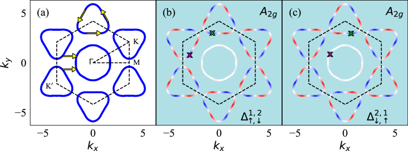
Figure 19: (a) Fermi surface in absence of Ising SOC. Yellow arrows represent the nesting vectors. (b,c) Leading solution of the linearized gap equation ($\Delta^{1,2}_{\uparrow,\downarrow}(\mathbf{k}_{F})$ , $\Delta_{2,1}^{\downarrow,\uparrow}(\mathbf{k}_{F})$) plotted on the Fermi surface in absence of Ising SOC. Additional parameters: $U=1.0$, $J=U/4$. Cross represent nesting vectors connecting gap on Fermi surface.

The observed dominance of the nodal pairing structure can be attributed to the nesting properties of the Fermi surface. As shown in Figure 2(c) of the main text, a pronounced peak in susceptibility is observed around 0.4$\Gamma$M. This momentum vector aligns closely with the intra-pocket nesting vectors depicted by the yellow arrows in Fig 19(a). While inter-pocket nesting vectors connecting the $K$ and $\Gamma$ pockets exist, their relative scarcity suggests a negligible contribution. These dominant intra-pocket nesting vectors favor a strong pairing interaction within the $K$ pocket, leading to the observed nodal pairing structure, while the $\Gamma$-centered pocket exhibits a weaker pairing strength.

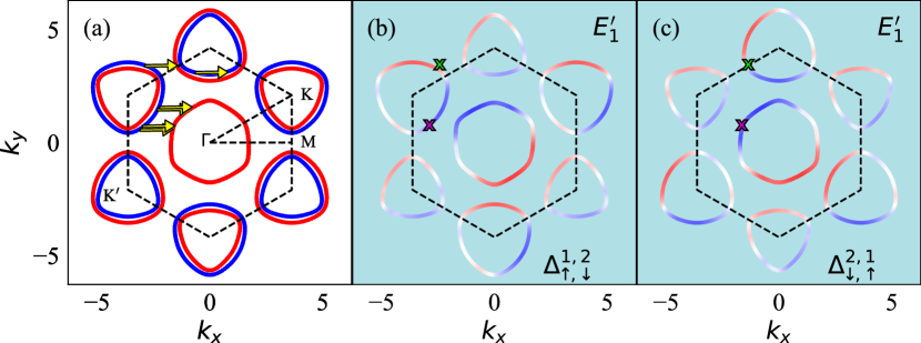
Figure 20: (a) Spin split Fermi surface in presence of Ising SOC. For clarity, the $\Gamma$-centered pocket associated with up spin (blue) is not shown here.. Yellow arrows represent the nesting vectors. (b,c) Leading solution of the linearized gap equation ($\Delta^{1,2}_{\uparrow,\downarrow}(\mathbf{k}_{F})$ , $\Delta_{2,1}^{\downarrow,\uparrow}(\mathbf{k}_{F})$) plotted on the Fermi surface in presence of Ising SOC. Additional parameters: $U=1.0$, $J=U/4$. Cross represent nesting vectors connecting gap on Fermi surface.

Like before a pronounced peak in susceptibility is observed around 0.4$\Gamma$M, as shown in Figure 2(d) of the main text. However, due to the spin-splitting of the Fermi surface induced by Ising SOC, the $K$ and $\Gamma$ pockets exhibit a more pronounced curvature. This enhanced curvature facilitates the emergence of additional inter-pocket nesting vectors connecting these pockets. Consequently, in contrast to the scenario without Ising SOC, a significant pairing interaction now develops within the $\Gamma$-centered pocket.

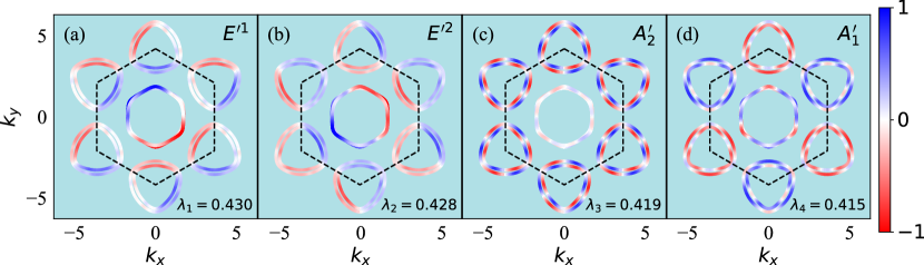
Figure 21: Solutions of the linearized gap equation, $\Delta(\mathbf{k}_{F})$, plotted on the spin-split Fermi surface(D_3h symmetry) for the four leading superconducting pairing gaps with corresponding eigenvalue $\lambda$. The non-interacting Hamiltonian used here neglects the Ising SOC and assumes D_6h symmetry. Additional parameters: $U=1.0$, $J=U/4$.

Figure 21 presents the solutions of the linearized gap equation for a enforced spin-split Fermi surface with D_3h symmetry and a pairing interaction calculated from a non-interacting Hamiltonian that neglects Ising SOC, thereby preserving its inherent D_6h symmetry. These results demonstrate that the spin-splitting of the Fermi points induced by Ising SOC is sufficient to drive the system towards a dominant spin-triplet pairing instability.

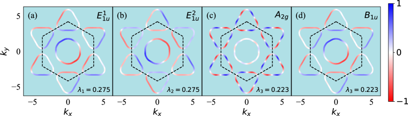
Figure 22: Solutions of the linearized gap equation, $\Delta(\mathbf{k}_{F})$, plotted on the Fermi surface (D_6h symmetry) for the four leading superconducting pairing gaps with corresponding eigenvalues ($\lambda$). Notably, the non-interacting Hamiltonian employed here incorporates the Ising SOC. Additional parameters used are $U=1.0$ and $J=U/4$.

Unlike before in Figure 21 we present the solutions of the linearized gap equation for a Fermi surface with D_6h symmetry and a pairing interaction calculated from a non-interacting Hamiltonian that takes into account of Ising SOC, thereby reducing its symmetry to D_3h symmetry. Here also the system gets driven towards a dominant spin-triplet pairing instability.

Our main work incorporated the effects of Ising SOC within both the non-interacting Hamiltonian and the Fermi surface. This comprehensive treatment led to results that differ at the subdominant level of the order parameter. In the main work, the leading subdominant order parameter was identified as a (s+f) singlet-triplet mixture, whereas here, we get an (i+f) singlet-triplet mixture.