Large gap probabilities of complex and symplectic
spherical ensembles with point charges

Abstract.

We consider $n$ eigenvalues of complex and symplectic induced spherical ensembles, which can be realised as two-dimensional determinantal and Pfaffian Coulomb gases on the Riemann sphere under the insertion of point charges. For both cases, we show that the probability that there are no eigenvalues in a spherical cap around the poles has an asymptotic behaviour as $n\to\infty$ of the form

$$\exp\Big{(}c_{1}n^{2}+c_{2}n\log n+c_{3}n+c_{4}\sqrt{n}+c_{5}\log n+c_{6}+\mathcal{O}(n^{-\frac{1}{12}})\Big{)}$$

and determine the coefficients explicitly. Our results provide the second example of precise (up to and including the constant term) large gap asymptotic behaviours for two-dimensional point processes, following a recent breakthrough by Charlier.

1. Introduction and main results

1.1. Spherical ensembles

We consider two-dimensional Coulomb gases [63] (also known as one-component plasmas) $\boldsymbol{x}=\{x_{j}\}_{j=1}^{n}$ on the Riemann sphere $\mathbb{S}=\{x\in\mathbb{R}^{3}:\|x\|=1\}$, under the insertion of point charges at the south and north poles, ${\rm{S}}=(0,0,-1)$ and ${\rm{N}}=(0,0,1)$ respectively. Here, $\|\cdot\|$ is the Euclidean metric in $\mathbb{R}^{3}$. In addition to the point charge insertions, we consider both determinantal and Pfaffian Coulomb gases. Consequently, for given fixed non-negative integers $\alpha$ and $c$ determining point charges at the poles, the joint probability distributions of the models are given by

(1.1) $$d\boldsymbol{\mathcal{P}}_{n}^{\mathbb{C}}(\boldsymbol{x}) =\frac{1}{\mathcal{Z}_{n}^{\mathbb{C}}}\prod_{j>k=1}^{n}\|x_{j}-x_{k}\|^{2}\prod_{j=1}^{n}\|x_{j}-{\rm{N}}\|^{2\alpha}\,\|x_{j}-{\rm{S}}\|^{2c}\,dA_{\mathbb{S}}(x_{j}),$$

(1.2) $$d\boldsymbol{\mathcal{P}}_{n}^{\mathbb{H}}(\boldsymbol{x}) =\frac{1}{\mathcal{Z}_{n}^{\mathbb{H}}}\prod_{j>k=1}^{n}\|x_{j}-x_{k}\|^{2}\|x_{j}-\overline{x}_{k}\|^{2}\prod_{j=1}^{n}\|x_{j}-\overline{x}_{j}\|^{2}\|x_{j}-{\rm{N}}\|^{4\alpha}\,\|x_{j}-{\rm{S}}\|^{4c}\,dA_{\mathbb{S}}(x_{j}),$$

where $dA_{\mathbb{S}}$ is the area measure on $\mathbb{S}$, and we use the convention $\overline{x}=(x_{1},-x_{2},x_{3})$ for $x=(x_{1},x_{2},x_{3})$. Here, $\mathcal{Z}_{n}^{\mathbb{C}}$ and $\mathcal{Z}_{n}^{\mathbb{H}}$ are partition functions that make $\boldsymbol{\mathcal{P}}_{n}^{\mathbb{C}}$ and $\boldsymbol{\mathcal{P}}_{n}^{\mathbb{H}}$ probability measures. The superscripts $\mathbb{C}$ and $\mathbb{H}$ denoting determinantal and Pfaffian Coulomb gases, respectively, will become clear below.

For readers who are inclined towards the statistical physics perspective, it suffices to regard (1.1) and (1.2) as the primary subjects of our investigations. On the other hand, for readers from the random matrix theory community, let us stress that these models have realisations of eigenvalues of random matrix models called complex [61, 64, 77] and symplectic [28, 65, 87, 88] spherical induced ensembles. We refer to [26, Section 2.5] and [27, Section 6.3] for comprehensive reviews, see also a recent work [91] and references therein. A simple way to define these random matrix models is as $n\times n$ complex or quaternion matrices, denoted by G, whose matrix probability distribution function is proportional to

(1.3) $$\frac{\det(\textbf{G}\textbf{G}^{*})^{c\beta/2}}{\det(\mathbbm{1}_{n}+\textbf{G}\textbf{G}^{*})^{(2n+c+\alpha)\beta/2}},\qquad\beta=\begin{cases}2&\textup{for the complex case},\vskip 3.0pt plus 1.0pt minus 1.0pt\\ 4&\textup{for the quaternionic case}.\end{cases}$$

For the special case when $c=\alpha=0$ (i.e. without point charges), these models are called the complex and symplectic spherical ensembles. In this case, an element-wise realisation of random matrices distributed as (1.3) is due to Krishnapur [77]. To be more concrete, the matrix distribution (1.3) follows from $\textbf{G}_{1}\textbf{G}_{2}^{-1}$, where $\textbf{G}_{1}$ and $\textbf{G}_{2}$ are independent complex or symplectic Ginibre matrices whose elements are given by i.i.d. complex or quaternionic Gaussian random variables. It is evident from the construction that the spherical ensembles are closely related to generalised eigenvalue problems [65, 54], which find applications in random plane geometry. Beyond the spherical cases, the presence of point charges can also be realised at the level of matrix models via a so-called inducing procedure, see e.g. [61, 88, 60]. This construction requires the use of rectangular Ginibre matrices as well as Haar-distributed matrices within the symmetry classes under consideration. In this inducing procedure, one needs to assume that $\alpha$ and $c$ are non-negative integer values since they are related to the rectangular parameters.

It follows from (1.3) that the joint distributions of eigenvalues $\boldsymbol{z}=\{z_{j}\}_{j=1}^{n}$ are given by

(1.4) $$d\mathbf{P}_{n}^{\mathbb{C}}(\boldsymbol{z}) =\frac{1}{Z_{n}^{\mathbb{C}}}\prod_{j>k=1}^{n}|z_{j}-z_{k}|^{2}\prod_{j=1}^{n}e^{-nQ_{n}(z_{j})}\,dA(z_{j}),$$

(1.5) $$d\mathbf{P}_{n}^{\mathbb{H}}(\boldsymbol{z}) =\frac{1}{Z_{n}^{\mathbb{H}}}\prod_{j>k=1}^{n}|z_{j}-z_{k}|^{2}|z_{j}-\overline{z}_{k}|^{2}\prod_{j=1}^{n}|z_{j}-\overline{z}_{j}|^{2}e^{-2nQ_{n}(z_{j})}\,dA(z_{j}),$$

where $dA(z)=d^{2}z/\pi$ and the external potential $Q_{n}$ is given by

(1.6) $$Q_{n}(z):=\frac{n+\alpha+c+1}{n}\log(1+|z|^{2})-\frac{2c}{n}\log|z|.$$

The models (1.4) and (1.5) are again two-dimensional Coulomb gas ensembles in the complex plane, with an $n$-dependent potential. Due to their special integrable structures, they are determinantal and Pfaffian Coulomb gas ensembles, respectively. We mention that the partition functions $Z_{n}^{\mathbb{C}}$ and $Z_{n}^{\mathbb{H}}$ can be expressed in terms of the gamma functions as

(1.7) $$Z_{n}^{\mathbb{C}}=n!\prod_{k=0}^{n-1}\frac{\Gamma(k+c+1)\Gamma(n+\alpha-k)}{\Gamma(n+\alpha+c+1)},\qquad Z_{n}^{\mathbb{H}}=n!\,2^{n}\,\prod_{k=0}^{n-1}\frac{\Gamma(2k+2c+2)\Gamma(2n+2\alpha-2k)}{\Gamma(2n+2\alpha+2c+2)}.$$

To observe the equivalence between (1.1) and (1.4), as well as (1.2) and (1.5), recall that the stereographic projection $\phi:\mathbb{S}^{2}\to\mathbb{C}\cup\{\infty\}$ is given by

(1.8) $$\phi(x)=\begin{cases}\dfrac{x_{1}+ix_{2}}{1-x_{3}},&\textup{if }x\in\mathbb{S}^{2}\setminus{\rm{N}},\vskip 3.0pt plus 1.0pt minus 1.0pt\\ \infty,&\textup{if }x={\rm{N}},\end{cases}\qquad\phi^{-1}(z)=\Big{(}\frac{2\operatorname{Re}z}{1+|z|^{2}},\frac{2\operatorname{Im}z}{1+|z|^{2}},\frac{|z|^{2}-1}{1+|z|^{2}}\Big{)},$$

where $x=(x_{1},x_{2},x_{3}).$ Using these, one can easily check that the measures (1.1) and (1.2) are a pull-back of (1.4) and (1.5), whence the name spherical for the random matrix G was first coined [77, 64]. Furthermore, the partition functions $\mathcal{Z}_{n}^{\mathbb{C}}$ and $\mathcal{Z}_{n}^{\mathbb{H}}$ in (1.1) and (1.2) are also given by (1.7), up to explicit constants. From this viewpoint, the potential (1.6) in the complex plane can also be realised as point charge insertions at the origin and infinity, cf. [93].

The potential $Q_{n}$ in (1.6) is indeed a prominent example of weakly confining potential, see e.g. [25] and references therein. Contrary to Coulomb gas ensembles with a confining potential that makes the particles lie in a compact set in the large-$n$ limit, the ensembles (1.4) and (1.5) tend to be distributed in the whole complex plane. To be more precise, due to the Laplacian growth property of the two-dimensional Coulomb gas ensemble, for given fixed $\alpha$ and $c$, the ensembles (1.4) and (1.5) tend to occupy the whole complex plane with the limiting density

(1.9) $$\rho^{\rm sp}(z)=\frac{1}{(1+|z|^{2})^{2}}.$$

As a consequence, using the inverse stereographic projection, we infer that as $n\to\infty$, the ensembles (1.1) and (1.2) tend to be uniformly distributed on the whole Riemann sphere $\mathbb{S}$, see Figure 1. We also mention that the equilibrium measure problems associated with spherical Coulomb gases with point charges have been recently studied in [83, 43].

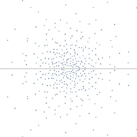
(a) $\{z_{j}\}_{j=1}^{n}$, $z_{j}\in\mathbb{C}$

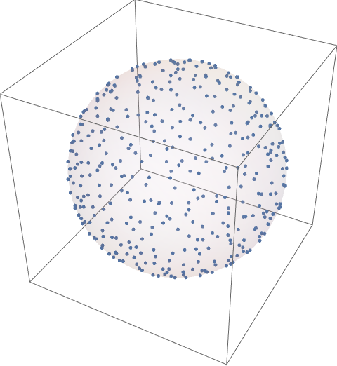
(b) $\{x_{j}\}_{j=1}^{n}$, $x_{j}\in\mathbb{S}$

Figure 1. The plot (A) displays eigenvalues of the spherical symplectic ensembles, where $n=200$. The plot (B) shows its projection to the sphere.

1.2. Main results: large gap probabilities

In this work, we study the asymptotic behaviour of the large gap probabilities as $n\to\infty$ of the ensembles (1.4) and (1.5):

(1.10) $$\begin{split}\mathcal{P}_{n}(R;\alpha,c)&:=\mathbb{P}\Big{[}\textup{there is no eigenvalues in }\mathbb{D}(0,R)\Big{]}.\end{split}$$

This problem was already considered a decade ago in the work [3], where the leading term for the complex case with $\alpha=c=0$ was obtained (i.e. the constant $A_{1}$ in Theorem 1.1).

More generally, obtaining large gap asymptotics is a classical and challenging problem in random matrix theory with a long history, which has attracted considerable attention over the years. The literature pertaining to this topic will be reviewed in Subsection 1.3 below. Note that $\mathcal{P}_{n}$ can also be written as

(1.11) $$\mathcal{P}_{n}(R;\alpha,c)=\mathbb{P}\Big{[}\min\{|z_{1}|,\ldots,|z_{n}|\}\geq R\,\Big{]}.$$

Hence $\mathcal{P}_{n}$ can be viewed as a heavy-tail distribution for the distribution of the smallest moduli. Analogous extreme distributions have been widely studied for various one-dimensional log-correlated point processes (such as the Tracy-Widom distribution for the Airy point process); this will be discussed in Subsection 1.3.4. In our case, the moduli $\{|z_{j}|\}_{j=1}^{n}$ forms a permanantal point process (see e.g. [7]), and the quantity $\mathcal{P}_{n}$ can also be interpreted as the large deviation probability of this process. Furthermore, $\mathcal{P}_{n}$ is intimately connected to an energy minimisation (electrostatics) problem, which is a fundamental aspect of potential theory, see Subsection 1.3.2. Additionally, it is equivalent to the free energy of a one-component plasma confined by hard walls, see Subsection 1.3.3 for further details.

For the models (1.1) and (1.2) on the sphere, the probability (1.10) coincides with the probability that there are no particles in a spherical cap (whose center is the south pole) of area

(1.12) $$4\pi\frac{R^{2}}{1+R^{2}},$$

see Figure 3 for some illustrations. Note that instead of (1.10), one may also consider

(1.13) $$\begin{split}\widetilde{\mathcal{P}}_{n}(R;\alpha,c)&:=\mathbb{P}\Big{[}\textup{there is no eigenvalues in }\mathbb{D}(0,R)^{c}\Big{]}=\mathbb{P}\Big{[}\max\{|z_{1}|,\ldots,|z_{n}|\}\leq R\,\Big{]}.\end{split}$$

Due to the sphere geometry, there is a duality relation between $\mathcal{P}_{n}$ and $\widetilde{\mathcal{P}}_{n}$:

(1.14) $$\mathcal{P}_{n}(R;\alpha,c)=\widetilde{\mathcal{P}}_{n}(1/R;c,\alpha).$$

Alternatively, (1.14) can also be directly obtained using Lemma 2.1 below.

In the sequel, we add the superscripts and write $\mathcal{P}_{n}^{\mathbb{C}}$ and $\mathcal{P}_{n}^{\mathbb{H}}$ to distinguish (1.4) and (1.5). To state our main results, we need some elementary special functions. Recall that the complementary error function is defined by [92, Chapter 7]

(1.15) $$\operatorname{erfc}(z):=\frac{2}{\sqrt{\pi}}\int_{z}^{\infty}e^{-t^{2}}\,dt$$

and that the Barnes $G$-function is defined recursively by [92, Section 5.17]

(1.16) $$G(z+1)=\Gamma(z)G(z),\qquad G(1)=1,$$

where $\Gamma$ is the standard gamma function. We write

(1.17) $$\mathcal{I}_{1} =\sqrt{2}\int_{-\infty}^{0}\log\Big{(}\tfrac{1}{2}\operatorname{erfc}(t)\Big{)}\,dt+\sqrt{2}\int_{0}^{\infty}\bigg{[}\log\Big{(}\tfrac{1}{2}\operatorname{erfc}(t)\Big{)}+t^{2}+\log t+\log(2\sqrt{\pi})\bigg{]}\,dt\approx-2.301,$$

(1.18) $$\mathcal{I}_{2} =\int_{-\infty}^{\infty}\bigg{[}\frac{(1+t^{2})e^{-t^{2}}}{\sqrt{\pi}\operatorname{erfc}(t)}-\Big{(}t^{3}+\frac{3}{2}t\Big{)}\mathbbm{1}_{(0,\infty)}(t)\bigg{]}\,dt\approx 0.928.$$

We are now ready to state the asymptotics as $n\to\infty$ of the large gap probabilities of the complex induced spherical ensemble (1.4).

Theorem 1.1 (Large gap probabilities of the complex ensemble).

Let $\alpha,c\in\mathbb{Z}_{\geq 0}$ and $R>0$ be fixed. Then as $n\to\infty$, we have

(1.19) $$\log\mathcal{P}_{n}^{\mathbb{C}}(R;\alpha,c)=A_{1}n^{2}+A_{2}n\log n+A_{3}n+A_{4}\sqrt{n}+A_{5}\log n+A_{6}+\mathcal{O}(n^{-\frac{1}{12}}),$$

where

(1.20) $$A_{1} =\frac{1}{2}\Big{(}\frac{R^{2}}{1+R^{2}}-\log(1+R^{2})\Big{)},$$

(1.21) $$A_{2} =-\frac{1}{2}\frac{R^{2}}{1+R^{2}},$$

(1.22) $$A_{3} =\frac{R^{2}}{1+R^{2}}\Big{(}1+\alpha+c-\frac{1}{2}\log(2\pi)-\log R\Big{)}-\alpha\log(1+R^{2}),$$

(1.23) $$A_{4} =\frac{R}{1+R^{2}}\,\mathcal{I}_{1},$$

(1.24) $$A_{5} =\frac{1+\alpha+c}{2(1+R^{2})}-\frac{1}{6}-\frac{\alpha+c^{2}}{2},$$

(1.25) $$\begin{split}A_{6}&=\Big{(}\frac{1+\alpha+c}{1+R^{2}}-\frac{1}{3}-\alpha-c^{2}\Big{)}\log R-\frac{\alpha^{2}-c^{2}}{2}\log(1+R^{2})\\ &\quad+\Big{(}\frac{1}{2}-(1+\alpha+c)\frac{R^{2}}{1+R^{2}}\Big{)}\frac{\log(2\pi)}{2}+\frac{(\alpha+c)(1+\alpha+c)}{2}\frac{R^{2}}{1+R^{2}}\\ &\quad-\frac{2}{3}\frac{1-R^{2}}{1+R^{2}}\,\mathcal{I}_{2}+\frac{1}{12}\Big{(}1+\frac{11}{1+R^{2}}\Big{)}-\zeta^{\prime}(-1)+\log G(c+1).\end{split}$$

Here, $\zeta$ is the Riemann zeta function, $G$ is the Barnes $G$-function, and the constants $\mathcal{I}_{1}$ and $\mathcal{I}_{2}$ are given by (1.17) and (1.18).

Remark 1.2 (Conjecture for the terms proportional to $n\log n$ and $\sqrt{n}$).

In view of Theorem 1.1 and [34, Theorem 1.7], we formulate the following conjecture for $A_{2}$ and $A_{4}$, valid for a general radially symmetric potential $V$ such that $\{z\in\mathbb{C}:|z|<R\}$ is contained in the droplet:

(1.26) $$A_{2}=-\frac{1}{2}\int_{|z|<R}\,d\sigma_{V}(z)\qquad\mbox{and}\qquad A_{4}=R\sqrt{\rho(R)}\,\mathcal{I}_{1},$$

where $d\sigma_{V}=\Delta V\,dA=\rho\,dA$ is the equilibrium measure (1.39) associated with the potential $V$, see also Subsection 1.3.2. This conjecture is consistent with Theorem 1.1, and also with the result [34, Theorem 1.7] on the Mittag-Leffler ensemble. In our case, $\rho$ is given by (1.9), whereas for the Mittag-Leffler ensemble, $\rho$ is given by (1.36).

As previously mentioned, when $\alpha=c=0$, $A_{1}$ was already obtained in [3, Proposition 3.1]. However, a more precise expansion has not been discovered; indeed even the second term $A_{2}$ is new to our knowledge.

The symplectic counterpart of Theorem 1.1 is as follows.

Theorem 1.3 (Large gap probabilities of the symplectic ensemble).

Let $\alpha,c\in\mathbb{Z}_{\geq 0}$ and $R>0$ be fixed. Then as $n\to\infty$, we have

(1.27) $$\log\mathcal{P}_{n}^{\mathbb{H}}(R;\alpha,c)=\widehat{A}_{1}n^{2}+\widehat{A}_{2}n\log n+\widehat{A}_{3}n+\widehat{A}_{4}\sqrt{n}+\widehat{A}_{5}\log n+\widehat{A}_{6}+\mathcal{O}(n^{-\frac{1}{12}}),$$

where

(1.28) $$\widehat{A}_{1} =\frac{R^{2}}{1+R^{2}}-\log(1+R^{2}),$$

(1.29) $$\widehat{A}_{2} =-\frac{1}{2}\frac{R^{2}}{1+R^{2}},$$

(1.30) $$\widehat{A}_{3} =\frac{R^{2}}{1+R^{2}}\Big{(}2+2\alpha+2c-\frac{1}{2}\log(4\pi)-\log R\Big{)}-\Big{(}2\alpha+\frac{1}{2}\Big{)}\log(1+R^{2}),$$

(1.31) $$\widehat{A}_{4} =\frac{1}{\sqrt{2}}\frac{R}{1+R^{2}}\,\mathcal{I}_{1},$$

(1.32) $$\widehat{A}_{5} =\frac{1+\alpha+c}{2(1+R^{2})}-\frac{5}{24}-\frac{\alpha+c}{2}-c^{2},$$

(1.33) $$\begin{split}\widehat{A}_{6}&=\Big{(}\frac{1+\alpha+c}{1+R^{2}}-\frac{5}{12}-\alpha-c-2c^{2}\Big{)}\log R-(\alpha-c)\Big{(}\frac{1}{2}+\alpha+c\Big{)}\log(1+R^{2})\\ &\quad-\Big{(}c+(1+\alpha+c)\frac{R^{2}}{1+R^{2}}\Big{)}\frac{\log(4\pi)}{2}+\Big{(}c+\frac{1}{4}\Big{)}\log 2+\Big{(}\frac{1}{2}+\alpha+c\Big{)}(1+\alpha+c)\frac{R^{2}}{1+R^{2}}\\ &\quad-\frac{1}{3}\frac{1-R^{2}}{1+R^{2}}\mathcal{I}_{2}+\frac{1}{24}\Big{(}1+\frac{11}{1+R^{2}}\Big{)}-2\zeta^{\prime}(-1)+\log\Big{(}G(c+1)G(c+\tfrac{3}{2})\Big{)}.\end{split}$$

Here, the constants $\mathcal{I}_{1}$ and $\mathcal{I}_{2}$ are given by (1.17) and (1.18).

The numerical verifications of Theorems 1.1 and 1.3 are provided in Figure 2. Here, we present the plots for the case where $\alpha=c=0$, and similar figures can be observed for other values of $\alpha$ and $c$.

In general, for Pfaffian point processes, the large gap problems have been much less developed, even in dimension one, see Subsection 1.3.4. Indeed, Theorem 1.3 provides one of the very few results on precise large gap asymptotics for Pfaffian point processes.

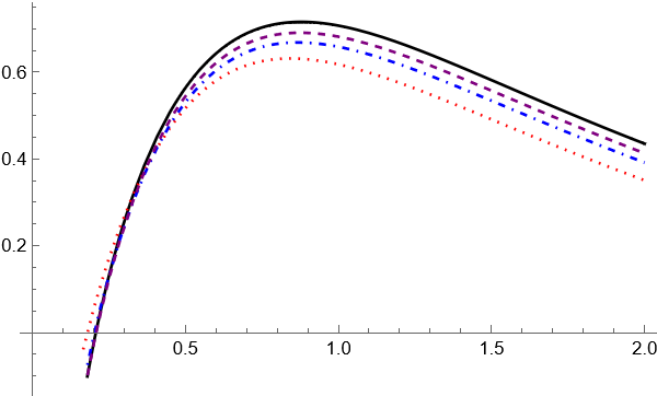
(a) Complex

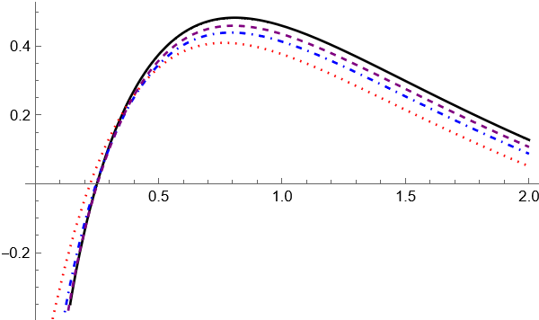
(b) Symplectic

Figure 2. The plot (A) shows $R\mapsto A_{6}$ (black full line) and its comparison $R\mapsto\log\mathcal{P}_{n}^{\mathbb{C}}(R;\alpha,c)-(A_{1}n^{2}+A_{2}n\log n+A_{3}n+A_{4}\sqrt{n}+A_{5}\log n),$ where $\alpha=c=0$. Here, $n=10$ (red, dotted line), $n=40$ (blue, dot-dashed line) and $n=160$ (purple, dashed line), cf. Lemma 2.1. The plot (B) shows the same figure for the symplectic case.

By comparing Theorems 1.1 and 1.3, one can observe

(1.34) $$2\,A_{1}=\widehat{A}_{1},\qquad A_{2}=\widehat{A}_{2}.$$

The agreement of the first two terms (up to a factor of 2 for the first term) turns out to be a universal feature of free energy expansions of determinantal and Pfaffian Coulomb gases. We refer the reader to [29], where such the same phenomenon was established for partition functions with soft edges.

1.3. Related works and further results

In this subsection, we shall discuss the progress made regarding large gap probabilities and related topics, providing further motivations for our study and elucidating our contributions to this direction. In addition, we present further consequences arising from our main results.

1.3.1. Large gap probabilities for the Ginibre ensemble

As previously mentioned, Ginibre matrices are non-Hermitian random matrices with i.i.d. Gaussian entries, see [26, 27] for recent reviews. The joint probability distributions of their eigenvalues are of the form (1.4) and (1.5), where the external potential is instead given by $|z|^{2}$. Its two-parameter extension, the Mittag-Leffler ensemble, has a potential of the form

(1.35) $$Q^{\rm ML}(z)=|z|^{2b}-\frac{2c}{n}\log|z|,\qquad(b>0,\,c>-1).$$

The associated limiting spectrum is a centred disc of radius $b^{-\frac{1}{2b}}$ and the density is given by

(1.36) $$\rho^{\rm ML}(z)=b^{2}|z|^{2b-2}.$$

In particular, if $b=1$, this gives rise to the well-known circular law.

An early study on the expansion of large gap probabilities of the complex Ginibre ensemble was due to Forrester [62], where he derived the first four terms in the expansion, i.e. $C_{j}$ ($j=1,2,3,4$) in (1.37) below. (See also [70, 71] for the first two terms). Subsequently, using the theory of skew-orthogonal polynomials, the symplectic counterpart was addressed in [8], where the authors obtained the first two terms, and partially conjectured the third one. (See also [9] for the extension to the product of Ginibre matrices.)

For a considerable period, obtaining a more precise expansion has been a longstanding open problem. It is only now that the specialised methods of asymptotic analysis required for this task have been mastered in the work [34] of Charlier. Consequently, it has been established that the large gap probabilities of the Mittag-Leffler ensemble take the form:

(1.37) $$\exp\Big{(}C_{1}n^{2}+C_{2}n\log n+C_{3}n+C_{4}\sqrt{n}+C_{5}\log n+C_{6}+\mathcal{O}(n^{-\frac{1}{12}})\Big{)}.$$

We mention that even though the large gap probabilities were stated in [34] only for the complex ensembles, the symplectic counterparts also follow by combining the results in [34] with [27, Proposition 5.10].

The key ingredient for the analysis of Charlier is a uniform asymptotic expansion of the incomplete gamma function due to Temme, see [98, Section 11.2.4] and [92, Section 8.12]. The basic concept of this method involves dividing the required summation based on different asymptotic regimes of the incomplete gamma function. Each division is meticulously chosen to minimise error bounds during asymptotic analysis, ensuring the smallest possible cumulative errors. Even though some of these ideas trace back to Forrester’s work [62] more than 30 years ago, their implementation demands technical mastery and a very systematic approach, particularly to achieve precision up to the constants $C_{5}$ and $C_{6}$ [34]. This method was also recently used in e.g. [33, 11] to obtain precise results on counting statistics.

Contrary to [34, 33, 11], the gap probability $\mathcal{P}_{n}$ is not expressed in terms of the incomplete gamma function but in terms of the incomplete beta function (cf. Lemma 2.1). This difference with [34, 33, 11] has far-reaching consequences in the proofs of Theorems 1.1 and  1.3. Indeed, our analysis requires very detailed asymptotics of the incomplete beta functions for various regimes of the parameters, and in particular we rely on some results in [98, Section 11.3.3]. We illustrate our proofs’ strategy in Figures 4 and  5 below. Interestingly, after a very detailed and intricate analysis, the resulting error bounds in Theorems 1.1 and  1.3 are $\mathcal{O}(n^{-\frac{1}{12}})$, i.e. of the same order as the bounds for the Mittag-Leffler ensemble (1.37). As a side note, one of the additional technical (or practical) difficulties in our work stems from a typo present in Temme’s original book [98, Section 11.3.3]. This typo is also present in NIST [92, Eq.(8.18.9)], and we are not aware of a literature where these typos have been reported, see Lemma 2.2 for the corrected version.

1.3.2. Leading order asymptotics and balayage measure

The leading order asymptotic behaviour of the large gap probabilities can alternatively be derived using a potential theoretic method [94] by investigating the associated balayage measure. For this purpose, let us recall that for a given probability measure $\mu$ on $\mathbb{C}$, the weighted logarithmic energy $I_{V}[\mu]$ associated with the external potential $V$ is given by

(1.38) $$I_{V}[\mu]:=\int_{\mathbb{C}^{2}}\log\frac{1}{|z-w|}\,d\mu(z)\,d\mu(w)+\int_{\mathbb{C}}V\,d\mu.$$

Assuming that $V$ is lower semi-continuous and finite on some set of positive capacity, $I_{V}[\mu]$ has a unique minimiser $\sigma_{V}$ with a support $S$ called the droplet. Furthermore, if $V$ is $C^{2}$-smooth in a neighbourhood of $S$, then $\sigma_{V}$ is absolutely continuous with respect to $dA$, and takes the form

(1.39) $$d\sigma_{V}(z)=\Delta V(z)\,\mathbbm{1}_{S_{V}}(z)\,dA(z),\qquad\Delta=\partial\bar{\partial}.$$

This property is often called the Laplacian growth, especially in the context of the Hele-Shaw flow. We now consider a gap $\Omega\subset\mathbb{C}$ and redefine the potential by

(1.40) $$V_{\Omega}(z)=\begin{cases}V(z)&\textup{if }z\not\in\Omega,\vskip 3.0pt plus 1.0pt minus 1.0pt\\ +\infty&\textup{if }z\in\Omega.\end{cases}$$

If $S\cap\Omega\neq\emptyset$, then the equilibrium measure associated with $V_{\Omega}$ is no longer absolutely continuous with respect to $dA$, but rather takes the form

(1.41) $$d\sigma_{V_{\Omega}}(z)=\Delta V(z)\,\mathbbm{1}_{S_{V}\setminus\Omega}(z)\,dA(z)+\nu(z)\,\mathbbm{1}_{\partial\Omega}(z)|dz|.$$

As the term balayage means sweeping in French, from an electrostatic perspective, the constraint that there are no particles in $\Omega$ pushes them to the boundary of $\Omega$ with a non-trivial distribution $\nu(z)$, cf. Figure 3. The balayage measure can be used to derive the leading order of the large gap probabilities. In particular, the leading order of the (logarithm of the) large gap probabilities is proportional to

(1.42) $$I_{V}[\sigma_{V}]-I_{V_{\Omega}}[\sigma_{V_{\Omega}}],$$

see e.g. [1, 44]. From a probabilistic point of view, the leading term (1.42) is a large deviation rate function, see e.g. [95]. An advantage of this approach is that it can be applied not only to the $\beta=2$ Coulomb gas ensembles but also to general $\beta>0$. However, for a general shape of domain, it is far from obvious to explicitly compute the balayage measure, and some non-trivial examples have been recently obtained in [2, 35]. On one hand, this approach usually has its limitations in deriving only the leading order asymptotic expansion.

In our present case, one can consider the balayage measure associated with the potential

(1.43) $$Q^{R}_{n}(z):=\begin{cases}+\infty&\textup{if }|z|\leq R,\vskip 3.0pt plus 1.0pt minus 1.0pt\\ Q_{n}(z)&\textup{if }|z|>R,\end{cases}$$

where $Q_{n}$ is given by (1.6). In this case, due to the rotational symmetry, the balayage measure becomes uniform distribution on $|z|=R$, see Figure 3. Then the leading order of our results also follows from computing the associated energy, see [35, Eq.(2.9)].

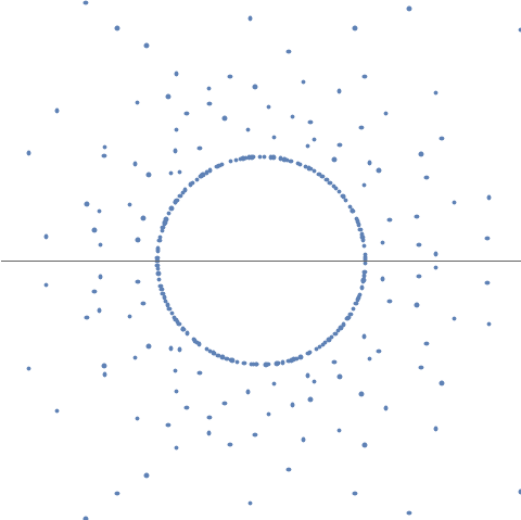
(a) $\{z_{j}\}_{j=1}^{n}$, $z_{j}\in\mathbb{C}$

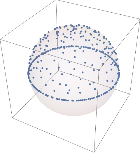
(b) $\{x_{j}\}_{j=1}^{n}$, $x_{j}\in\mathbb{S}$

Figure 3. The plot (A) displays eigenvalues of the spherical symplectic ensembles conditioned to have a gap $\{z\in\mathbb{C}:|z|<1\}$, where $n=200$. The plot (B) shows its projection to the sphere.

Let us also mention that beyond the two-dimensional Coulomb gases, the zeros of Gaussian analytic functions have been studied in the literature, see e.g. [68] and references therein. A characteristic feature when conditioning on a hole event for this model is that it produces a macroscopic region outside the hole region [69]. Such a forbidden region has been further investigated in recent literature [90].

1.3.3. Partition functions for two-dimensional point processes

For a given external potential $V$, the partition functions of determinantal and Pfaffian Coulomb gases are given by

(1.44) $$Z_{n,V}^{\mathbb{C}} :=\int_{\mathbb{C}^{n}}\prod_{j>k=1}^{n}|z_{j}-z_{k}|^{2}\prod_{j=1}^{n}e^{-n\,V(z_{j})}\,dA(z_{j}),$$

(1.45) $$Z_{n,V}^{\mathbb{H}} :=\int_{\mathbb{C}^{n}}\prod_{j>k=1}^{n}|z_{j}-z_{k}|^{2}|z_{j}-\overline{z}_{k}|^{2}\prod_{j=1}^{n}|z_{j}-\overline{z}_{j}|^{2}e^{-2nV(z_{j})}\,dA(z_{j}),$$

respectively. The asymptotic expansion of the partition function stands as one of the cornerstones in Coulomb gas theory. For a regular potential $V$, substantial progress has been made in this direction [17, 31, 107, 79]. Furthermore, for comprehensive literature and the latest advancements, we refer the reader to [10, 29, 30, 95].

For the partition functions $Z_{n}^{\mathbb{C}}$ and $Z_{n}^{\mathbb{H}}$ of induced spherical ensembles, their asymptotic expansions can be derived from well-known formulas involving the Barnes $G$-function.

Proposition 1.4 (Free energy expansions of the induced spherical ensembles).

As $n\to\infty$, the following asymptotic expansion holds.

• (Complex ensemble) We have

  (1.46) $$\log Z_{n}^{\mathbb{C}}=\mathcal{A}_{1}n^{2}+\mathcal{A}_{2}n\log n+\mathcal{A}_{3}n+\mathcal{A}_{4}\sqrt{n}+\mathcal{A}_{5}\log n+\mathcal{A}_{6}+\mathcal{O}(n^{-1}),$$

  where

  $$\mathcal{A}_{1}=-\frac{1}{2},\qquad\mathcal{A}_{2}=\frac{1}{2},\qquad\mathcal{A}_{3}=\frac{\log(2\pi)}{2}-1-\alpha-c,\qquad\mathcal{A}_{4}=0,\qquad\mathcal{A}_{5}=\frac{\alpha^{2}+c^{2}}{2}+\frac{1}{3},$$

  $$\mathcal{A}_{6}=\frac{\log(2\pi)}{2}-\frac{1}{12}+2\zeta^{\prime}(-1)-\frac{1}{2}(\alpha+c)(\alpha+c+1-\log(2\pi))-\log\Big{(}G(\alpha+1)G(c+1)\Big{)}.$$

• (Symplectic ensemble) We have

  (1.47) $$\log Z_{n}^{\mathbb{H}}=\widehat{\mathcal{A}}_{1}n^{2}+\widehat{\mathcal{A}}_{2}n\log n+\widehat{\mathcal{A}}_{3}n+\widehat{\mathcal{A}}_{4}\sqrt{n}+\widehat{\mathcal{A}}_{5}\log n+\widehat{\mathcal{A}}_{6}+\mathcal{O}(n^{-1}),$$

  where

  $$\widehat{\mathcal{A}}_{1}=-1,\qquad\widehat{\mathcal{A}}_{2}=\frac{1}{2},\qquad\widehat{\mathcal{A}}_{3}=\frac{\log(4\pi)}{2}-2-2\alpha-2c,\qquad\widehat{\mathcal{A}}_{4}=0,\qquad\widehat{\mathcal{A}}_{5}=\alpha^{2}+\frac{\alpha}{2}+c^{2}+\frac{c}{2}+\frac{5}{12},$$

  $$\begin{split}\widehat{\mathcal{A}}_{6}&=\log(2\pi)-\frac{13}{24}+4\zeta^{\prime}(-1)-(\alpha+c)(\alpha+c+\tfrac{3}{2}-\log(2\pi))-\log\Big{(}G(\alpha+1)G(\alpha+\tfrac{3}{2})G(c+1)G(c+\tfrac{3}{2})\Big{)}.\end{split}$$

For the complex case, we also refer to [61, 74]. See also [18] and references therein for the asymptotic behaviours of the logarithmic energy of the configurations.

Let us stress here that $\mathcal{A}_{4}=\widehat{\mathcal{A}}_{4}=0$. Such an absence of the $\mathcal{O}(\sqrt{n})$-term is a general feature of the free energy expansion for $\beta=2$ ensembles, see [29, 10] for the rotationally symmetric case and [30] for a non-rotationally symmetric example. Furthermore, note that for $\alpha=c=0$, we have

(1.48) $$\mathcal{A}_{5}\Big{|}_{\alpha=c=0}=\frac{1}{2}-\frac{\chi}{12},\qquad\widehat{\mathcal{A}}_{5}\Big{|}_{\alpha=c=0}=\frac{1}{2}-\frac{\chi}{24},$$

where $\chi=2$ is the Euler index of the droplet, in our case, the Riemann sphere. This form of the coefficient of the $\log n$ term was introduced in the work of Jancovici et al. [72, 97] and is expected to hold for more general droplets [29, 10, 30]. Note further that for $\alpha=c=0$, we have

(1.49) $$\mathcal{A}_{6}\Big{|}_{\alpha=c=0}=\frac{\log(2\pi)}{2}-\frac{1}{12}+\chi\,\zeta^{\prime}(-1),\qquad\widehat{\mathcal{A}}_{6}\Big{|}_{\alpha=c=0}=\frac{\log(2\pi)}{2}-\frac{13}{24}+\frac{\chi}{2}\Big{(}\frac{5\log 2}{12}+\zeta^{\prime}(-1)\Big{)}.$$

Here, again the $\chi$-dependent terms are expected to be universal, see [29]. Other than these $\chi$-dependent terms, the other parts of the $\mathcal{O}(1)$-term are related to the conformal geometric properties of the equilibrium measure, see e.g. the introduction of [30]. For the ensembles on the sphere with general radially symmetric potentials, the associated free energy expansions will be addressed in a forthcoming work.

Contrary to the regular case, when $V$ contains certain singularities, there has been less understanding of the asymptotic expansions. Among the various types of singularities one may consider, the following types are particularly noteworthy due to various motivations and have been extensively investigated in the literature.

• (Jump type singularity) This is the case where the weight function has a discontinuity. This type of singularity naturally arises in the context of the moment generating function of the disc counting function, see [33, 11, 12, 5, 38, 4] and references therein for recent progress. In particular, for the spherical ensembles, this has been addressed in a recent work [89].

• (Root type singularity) The pointwise root type singularity is equivalent to the point charge insertions. This type of singularities also finds application in the context of moments of characteristic polynomials [52, 102, 30]. We also refer to [15, 78, 80, 81, 82, 20, 21, 16] for extensive studies on the associated orthogonal polynomials. On the other hand, the circular (or non-isolated in general) root type singularity naturally arises in the context of the truncations of Haar unitary matrices [108, 13] or finite-rank perturbation [67].

• (Hard wall type singularity) This is the type we are exploring in our present work, namely the potential takes the form (1.40). While one might consider it as another jump type singularity, unlike the one seen in counting statistics, in the context of gap probabilities, the potential reveals an extreme discontinuity as it takes the value $+\infty$ in a certain region. As far as we are aware, the only instance prior to our current work where the partition function expansion, up to the constant term, was achieved for two-dimensional point processes, is the work [34] of Charlier.

In the context we have discussed, our main results can then be stated as free energy expansions of the partition functions (1.44) and (1.45), associated with the potential (1.6), which exhibits both root and hard wall type singularities.

Corollary 1.5 (Free energy expansions with singularities).

Let

(1.50) $$\mathsf{A}_{j}=A_{j}+\mathcal{A}_{j},\qquad\widehat{\mathsf{A}}_{j}=\widehat{A}_{j}+\widehat{\mathcal{A}}_{j},\qquad(j=1,2,\dots,6),$$

where $A_{j}$ and $\widehat{A}_{j}$ are given in Theorems 1.1 and  1.3 respectively, and $\mathcal{A}_{j}$ and $\widehat{\mathcal{A}}_{j}$ are given in Proposition 1.4. Let $V=Q^{R}$, where $Q^{R}$ is given by (1.43). Then as $n\to\infty$, we have

(1.51) $$\log Z_{n,V}^{\mathbb{C}} =\mathsf{A}_{1}n^{2}+\mathsf{A}_{2}n\log n+\mathsf{A}_{3}n+\mathsf{A}_{4}\sqrt{n}+\mathsf{A}_{5}\log n+\mathsf{A}_{6}+\mathcal{O}(n^{-\frac{1}{12}}),$$

(1.52) $$\log Z_{n,V}^{\mathbb{H}} =\widehat{\mathsf{A}}_{1}n^{2}+\widehat{\mathsf{A}}_{2}n\log n+\widehat{\mathsf{A}}_{3}n+\widehat{\mathsf{A}}_{4}\sqrt{n}+\widehat{\mathsf{A}}_{5}\log n+\widehat{\mathsf{A}}_{6}+\mathcal{O}(n^{-\frac{1}{12}}).$$

Proof.

Note that by the definition of $Q^{R}$ in (1.43), we have

(1.53) $$\mathcal{P}_{n}^{\mathbb{C}}(R;\alpha,c)=\frac{Z_{n,V}^{\mathbb{C}}}{Z_{n}^{\mathbb{C}}},\qquad\mathcal{P}_{n}^{\mathbb{H}}(R;\alpha,c)=\frac{Z_{n,V}^{\mathbb{H}}}{Z_{n}^{\mathbb{H}}}.$$

Then the corollary immediately follows from Theorems 1.1,  1.3 and Proposition 1.4. ∎

Contrary to the regular case stated in Proposition 1.4 or in e.g. [29, 30, 10], in Corollary 1.5, a non-trivial coefficient of the $\mathcal{O}(\sqrt{n})$-term does arise when considering the hard wall constraints of the potential. This is due to the hard wall constraints of the potential.

1.3.4. Large gap probabilities for one-dimensional point processes

Comparing with two-dimensional point processes, there have been far more investigations into the gap probabilities for one-dimensional point processes. For the reader’s convenience, let us list some of the literature.

Some early works where the leading order term of large gap probabilities for the eigenvalues of classical Hermitian random matrices include [19, 46, 47, 73, 84, 85, 101, 66]. Some of these works also find interesting connections with spin glass model as well as free fermionic systems. As in the two-dimensional cases, the leading order can be obtained using potential-theoretic computations, sometimes referred to as the Coulomb gas method.

For determinantal point processes, large gap problems can be interpreted as asymptotic expansions for structured determinants. For one-dimensional point processes, the Riemann-Hilbert approach has been particularly successful in obtaining precise asymptotic behaviours. (On the other hand, in dimension two, developing a Riemann-Hilbert approach to large gap problems breaking the radial symmetry is still an outstanding open problem.) However, multiplicative constants of large gap problems are in general very difficult to obtain and are still open in some cases (see below).

• (Hankel determinants) The form of the asymptotic expansion depends on the external potential of the Hermitian random unitary matrices, particularly on their edge behaviours of the associated equilibrium measure. For the generalised Gaussian unitary ensembles, a general result can be found in [51, 36], and for the Laguerre and Jacobi types, these can be found in [37]. Furthermore, the large gap asymptotics of the Muttalib-Borodin model with constant potential involve a generalisation of Hankel determinants and were established in [32].

• (Toeplitz determinants) For the circular unitary ensemble, the probability of an arc being empty of eigenvalues, up to a multiplicative constant, was obtained in [103]. This was later extended in [57, Proposition 1.1.3] to situations where the gap region consists of multiple arcs of the same length symmetrically located on the unit circle, and higher order correction terms were obtained in [86].

• (Fredholm determinants) In this case, the asymptotic expansions have been investigated for different limiting point processes.

  • (Sine point process) After the asymptotics of gap probabilities on a single interval were conjectured in [53], they were proved simultaneously and independently in [55, 75]. The case of several interval gaps was investigated in [104], where later the results were made more explicit in [48]. In particular, the oscillations were expressed in terms of Jacobi theta functions in [48] for the first time. Nonetheless, the multiplicative constant was still missing in [48]. For the two-interval case, this constant was recently obtained in [58].

  • (Airy point process) The conjecture on the large gap asymptotics made in [99] was shown in [49, 14] up to and including the multiplicative constant. For the case of two intervals, this was obtained in [22] without a multiplicative constant, which was later obtained in [76]. The gap probabilities in the bulk were also obtained in [23].

  • (Bessel point process) The large gap asymptotics on a single interval were obtained in [100] up to, but not including, the multiplicative constant. The multiplicative constant conjectured in [100] was later established in [56, 50] using different approaches. Recently, the case of several intervals has also been addressed in [24] with the multiplicative constants left undetermined.

  Beyond the standard limiting point processes, there have been further developments on other types of point processes. These include the Wright’s generalised Bessel and Meijer-$G$ point processes [41, 39, 40]; the Pearcey point process [45]; the hard edge Pearcey point process [105]; the tacnode point process [106]; and the Freud point process [42].

Organisation of the paper

The rest of this paper is organised as follows. In Section 2, we provide an outline of proofs together with necessary preliminaries. Section 3 is devoted to the analysis of the complex case, where we prove Theorem 1.1. Section 4 is for the symplectic counterpart, where we provide the proof of Theorem 1.3. Additionally, this article contains an appendix where we compile some tail asymptotic behaviours of the binomial distributions.

2. Outline of proofs

In this section, we provide the preliminaries and outline of proofs of our main results.

The key ingredients for the proofs are given as follows.

• We first obtain the expression of gap probabilities in terms of products of incomplete beta functions (Lemma 2.1). This follows from the determinantal/Pfaffian structures of the underlying models and recent development [6] on the planar skew-orthogonal polynomials.

• We make use of the uniform asymptotic behaviours of the incomplete beta function (Lemma 2.2). Although this formula is provided in Temme’s book [98, Section 11.3.3.2], it turns out that there is a typo that can be corrected. We note that the same typo appears in [92, Eq.(8.18.9)].

• The remainder of the proof entails the asymptotic analysis of the finite-$n$ expression utilising the uniform asymptotic behaviours of the incomplete beta function, see Figures 4 and  5. This constitutes the main aspect of our proofs, and we apply the method developed by Charlier [34, 33] to our model.

Figure 4. Illustration of the divisions of the summations in (2.19) and (3.22), together with lemmas on the asymptotic expansions in each sub-summation.

Figure 5. The analogue of Figure 4 for the symplectic counterpart, i.e. illustration of the summations in (2.21) and (4.13).

Before introducing the strategy in more detail, let us first provide the proof of Proposition 1.4.

Proof of Proposition 1.4.

By using the definition of the Barnes $G$-function, one can rewrite (1.7) as

(2.1) $$Z_{n}^{\mathbb{C}} =\frac{n!}{\Gamma(n+\alpha+c+1)^{n}}\frac{G(n+c+1)}{G(c+1)}\frac{G(n+\alpha+1)}{G(\alpha+1)},$$

(2.2) $$Z_{n}^{\mathbb{H}} =n!\Big{(}\frac{2^{2n+2\alpha+2c+1}}{\pi\Gamma(2n+2\alpha+2c+2)}\Big{)}^{n}\frac{G(n+c+1)}{G(c+1)}\frac{G(n+c+3/2)}{G(c+3/2)}\frac{G(n+\alpha+1)}{G(\alpha+1)}\frac{G(n+\alpha+3/2)}{G(\alpha+3/2)}.$$

Then the desired asymptotic expansion follows from the well-known asymptotic behaviours of the gamma function [92, Eq.(5.11.1)]

(2.3) $$\log N!=N\log N-N+\frac{1}{2}\log N+\frac{1}{2}\log(2\pi)+\frac{1}{12N}+\mathcal{O}\Big{(}\frac{1}{N^{3}}\Big{)},\qquad(N\to\infty)$$

and of the Barnes $G$-function [92, Eq.(5.17.5)]

(2.4) $$\begin{split}\log G(z+1)=\frac{z^{2}\log z}{2}-\frac{3}{4}z^{2}+\frac{\log(2\pi)z}{2}-\frac{\log z}{12}+\zeta^{\prime}(-1)-\frac{1}{240z^{2}}+\mathcal{O}\Big{(}\frac{1}{z^{4}}\Big{)},\qquad(z\to\infty).\end{split}$$

∎

Recall that the regularised incomplete beta function $I_{x}$ is given by

(2.5) $$I_{x}(a,b):=\frac{B_{x}(a,b)}{B(a,b)},\qquad B_{x}(a,b):=\int_{0}^{x}t^{a-1}(1-t)^{b-1}\,dt$$

where

(2.6) $$B(a,b)=B_{1}(a,b):=\frac{\Gamma(a)\Gamma(b)}{\Gamma(a+b)}$$

is the beta function, see [92, Chapter 8]. Note that by definition, we have

(2.7) $$I_{x}(a,b)=1-I_{1-x}(b,a).$$

We also note that for integer values $n\geq m$, we have

(2.8) $$I_{x}(m,n-m+1)=\sum_{j=m}^{n}\binom{n}{j}x^{j}(1-x)^{n-j}.$$

This in turn implies that the regularised incomplete beta function is the cumulative distribution function of the binomial distribution, i.e. for $X\sim B(n,p)$,

(2.9) $$\mathbb{P}(X\leq k)=I_{1-p}(n-k,k+1)=1-I_{p}(k+1,n-k).$$

In the following lemma, we express the gap probabilities in terms of the incomplete beta functions.

Lemma 2.1 (Evaluation of the gap probabilities at finite-$n$).

Let

(2.10) $$x=\frac{1}{1+R^{2}}.$$

Then we have

(2.11) $$\mathcal{P}_{n}^{\mathbb{C}}(R;\alpha,c) =\prod_{k=0}^{n-1}I_{x}(k+\alpha+1,n+c-k)=\prod_{k=0}^{n-1}I_{x}(n+\alpha-k,k+c+1),$$

(2.12) $$\mathcal{P}_{n}^{\mathbb{H}}(R;\alpha,c) =\prod_{k=0}^{n-1}I_{x}(2k+2\alpha+2,2n+2c-2k)=\prod_{k=0}^{n-1}I_{x}(2n+2\alpha-2k,2k+2c+2).$$

Proof.

Recall that $Q_{n}^{R}$ is given by (1.43). Let

(2.13) $$h_{k,m}:=\int_{\mathbb{C}}|z|^{2k}\,e^{-mQ_{n}(z)}\,dA(z),\qquad h_{k,m}(R):=\int_{\mathbb{D}(0,R)^{c}}|z|^{2k}\,e^{-mQ_{n}(z)}\,dA(z).$$

It follows from the general theory of determinantal and Pfaffian point processes that the associated partition functions (1.44) and (1.45) can be expressed in terms of (skew)-norms of the associated (skew)-orthogonal polynomials. Combining this with (1.53), we have

(2.14) $$\mathcal{P}^{\mathbb{C}}_{n}(R)=\prod_{k=0}^{n-1}\frac{h_{k,n}(R)}{h_{k,n}},\qquad\mathcal{P}^{\mathbb{H}}_{n}(R)=\prod_{k=0}^{n-1}\frac{h_{2k+1,2n}(R)}{h_{2k+1,2n}},$$

see e.g. [29, Eq.(1.37)]. In particular, we have used the construction of the skew-orthogonal polynomials [6, Corollary 3.3]. On the other hand, by using the Euler beta integrals, we have

$$h_{k,m}(R) =2\int_{R}^{\infty}\frac{r^{2k+1+2c\frac{m}{n}}}{(1+r^{2})^{(n+\alpha+c+1)\frac{m}{n}}}\,dr=\int_{R}^{\infty}\Big{(}\frac{r^{2}}{1+r^{2}}\Big{)}^{k+c\,\frac{m}{n}}\Big{(}\frac{1}{1+r^{2}}\Big{)}^{(n+\alpha+1)\,\frac{m}{n}-k-2}\frac{2r}{(1+r^{2})^{2}}\,dr$$

$$=\int_{0}^{x}t^{(n+\alpha+1)\,\frac{m}{n}-k-2}(1-t)^{k+c\,\frac{m}{n}}\,dt=B_{x}((n+\alpha+1)\,\tfrac{m}{n}-k-1,k+c\,\tfrac{m}{n}+1),$$

which gives

$$\frac{h_{k,n}(R)}{h_{k,n}}=I_{x}(n+\alpha-k,k+c+1),\qquad\frac{h_{2k+1,2n}(R)}{h_{2k+1,2n}}=I_{x}(2n+2\alpha-2k,2k+2c+2).$$

This completes the proof. ∎

To analyse the expressions in Lemma 2.1, it is convenient to introduce the notation

(2.15) $$N=\begin{cases}n+\alpha+c&\textup{ for the complex case,}\vskip 3.0pt plus 1.0pt minus 1.0pt\\ n+\alpha+c+\frac{1}{2}&\textup{ for the symplectic case.}\end{cases}$$

We further define

(2.16) $$k_{-}=\lfloor\delta N\rfloor-\alpha-1,\qquad k_{+}=\lceil(1-\delta)N\rceil-\alpha-1,$$

and

(2.17) $$k_{M}=\begin{cases}N-\lceil M\rceil-\alpha-1&\textup{ for the complex case,}\vskip 3.0pt plus 1.0pt minus 1.0pt\\ N-\lceil M\rceil-\alpha-\frac{3}{2}&\textup{ for the symplectic case.}\end{cases}$$

Here, we set

(2.18) $$M=N^{\frac{1}{3}}$$

and choose $\delta\in(0,\min\{x,1-x\})$ small enough so that $0<k_{-}<k_{+}<k_{M}<N$ holds for large $N$.

By using (2.16) and (2.17), we divide the sum in (2.11) by the following four parts:

(2.19) $$\log\mathcal{P}_{n}^{\mathbb{C}}(R;\alpha,c)=S_{0}+S_{1}+S_{2}+S_{3},$$

where

(2.20) $$S_{0} =\sum_{k=0}^{k_{-}}\log I_{x}(k+\alpha+1,n+c-k),\qquad S_{1}=\sum_{k=k_{-}+1}^{k_{+}-1}\log I_{x}(k+\alpha+1,n+c-k),$$

$$S_{2} =\sum_{k=k_{+}}^{k_{M}}\log I_{x}(k+\alpha+1,n+c-k),\qquad S_{3}=\sum_{k=k_{M}+1}^{n-1}\log I_{x}(k+\alpha+1,n+c-k).$$

Similarly, we divide the sum in (2.12) by

(2.21) $$\log\mathcal{P}_{n}^{\mathbb{H}}(R;\alpha,c)=\widehat{S}_{0}+\widehat{S}_{1}+\widehat{S}_{2}+\widehat{S}_{3},$$

where

(2.22) $$\widehat{S}_{0} =\sum_{k=0}^{k_{-}}\log I_{x}(2k+2\alpha+2,2n+2c-2k),\quad \widehat{S}_{1}=\sum_{k=k_{-}+1}^{k_{+}-1}\log I_{x}(2k+2\alpha+2,2n+2c-2k),$$

$$\widehat{S}_{2} =\sum_{k=k_{+}}^{k_{M}}\log I_{x}(2k+2\alpha+2,2n+2c-2k),\quad \widehat{S}_{3}=\sum_{k=k_{M}+1}^{n-1}\log I_{x}(2k+2\alpha+2,2n+2c-2k).$$

See Figures 4 and  5. As previously mentioned, the divisions in (2.20) and (2.22) are chosen in a way to minimise cumulative errors. For the asymptotic behaviours of $S_{0}$, $S_{2}$, and $S_{3}$, as well as $\widehat{S}_{0}$, $\widehat{S}_{2}$, and $\widehat{S}_{3}$, we can apply various tail behaviours of the binomial distribution (see Appendix A) together with a version of the Euler-Maclaurin formula (Lemma 3.3). The most technical part involves $S_{1}$ and $\widehat{S}_{1}$, which, from the viewpoint of the asymptotic behaviour of the incomplete beta function, are referred to as the symmetric regime. In this case, it is necessary to further divide the summations as in (3.22) and (4.13). For this regime, the following uniform asymptotics of the incomplete beta function play a key role.

Lemma 2.2 (Uniform asymptotics of the incomplete beta function).

Let $x_{0}=a/N$. Then as $N\to\infty$, we have

(2.23) $$I_{x}(a,N-a)=\frac{1}{2}\operatorname{erfc}\Big{(}-\eta\sqrt{\frac{N}{2}}\Big{)}+R_{a}(\eta),$$

where

(2.24) $$R_{a}(\eta)=e^{-\frac{1}{2}\eta^{2}N}\frac{1}{2\pi i}\int_{-\infty}^{\infty}e^{-\frac{1}{2}Nu^{2}}g(u)\,du.$$

Here, $\eta$ is given by

(2.25) $$-\frac{1}{2}\eta^{2}=x_{0}\log\Big{(}\frac{x}{x_{0}}\Big{)}+(1-x_{0})\log\Big{(}\frac{1-x}{1-x_{0}}\Big{)},\qquad\frac{\eta}{x-x_{0}}>0,$$

and $g$ is given by

(2.26) $$g(u)=\frac{dt}{du}\frac{1}{t-x}-\frac{1}{u+i\eta},$$

where the variables $t$ and $u$ are correlated by the bijection

(2.27) $$\frac{1}{2}u^{2}=x_{0}\log\Big{(}\frac{t}{x_{0}}\Big{)}+(1-x_{0})\log\Big{(}\frac{1-t}{1-x_{0}}\Big{)},\qquad\frac{\operatorname{Im}t}{u}>0,\qquad t\in\mathcal{L},$$

on

(2.28) $$\mathcal{L}=\Big{\{}t=\frac{\sin(\rho\sigma)}{\sin[(1+\rho)\sigma]}e^{i\sigma}:|\sigma|<\frac{\pi}{1+\rho}\Big{\}}\mapsto u\in\mathbb{R},\qquad\Big{(}\rho=\frac{x_{0}}{1-x_{0}}\Big{)}.$$

Furthermore, we have

(2.29) $$R_{a}(\eta)\sim\frac{1}{\sqrt{2\pi N}}e^{-\frac{1}{2}\eta^{2}N}\sum_{k=0}^{\infty}\frac{(-1)^{k}c_{k}(\eta)}{N^{k}}$$

uniformly for $x\in(0,1)$ and $x_{0}\in[\delta,1-\delta]$, where $0<\delta<\frac{1}{2}$ is an arbitrarily fixed small constant. Here, the coefficients $c_{n}(\eta)$ is given by

(2.30) $$c_{n}(\eta)=-i(2n-1)!!g_{2n},\qquad g_{n}=\frac{1}{n!}\frac{d^{n}}{du^{n}}g(u)\Big{|}_{u=0}.$$

In particular, the first two coefficients $c_{0}$ and $c_{1}$ are given by

(2.31) $$c_{0}(\eta) =\frac{1}{\eta}-\frac{\sqrt{x_{0}(1-x_{0})}}{x-x_{0}},$$

(2.32) $$c_{1}(\eta) =-\frac{1}{\eta^{3}}+\frac{1-13x_{0}+13x_{0}^{2}}{12\sqrt{x_{0}(1-x_{0})}}\frac{1}{x-x_{0}}+\frac{(1-2x_{0})\sqrt{x_{0}(1-x_{0})}}{(x-x_{0})^{2}}+\frac{(x_{0}(1-x_{0}))^{3/2}}{(x-x_{0})^{3}}.$$

All of the $c_{k}(\eta)$ are analytic at $\eta=0$.

Remark 2.3.

In [98, Section 11.3.3.2], the leading term of the right-hand side of (2.23) is incorrectly written as $\frac{1}{2}\operatorname{erfc}(-\eta\sqrt{\frac{N-a}{2}})$. The corrected version follows from the integral

$$e^{-\frac{1}{2}\eta^{2}N}\frac{1}{2\pi i}\int_{-\infty}^{\infty}e^{-\frac{1}{2}Nu^{2}}\frac{1}{u+i\eta}\,du=\frac{1}{2}\operatorname{erfc}\Big{(}-\eta\sqrt{\frac{N}{2}}\Big{)}.$$

This typo still appears in [92, Eq.(8.18.8)], where the first term of the right-hand side there should be corrected as

(2.33) $$I_{x}(a,b)\sim\frac{1}{2}\operatorname{erfc}\Big{(}-\eta\sqrt{\frac{a+b}{2}}\Big{)}.$$

The subleading terms in [98, 92] are correct. We note that the corrected version (2.23) can also be easily verified numerically.

3. Gap probabilities of the complex ensemble

In this section, we prove Theorem 1.1. As previously mentioned, we shall use the splitting (2.19). In Subsection 3.1, we perform the analysis of $S_{0}$, $S_{2}$ and $S_{3}$. Subsection 3.2 is devoted to the analysis of a more complicated part $S_{1}$, where we further need the division (3.22).

3.1. Analysis of $S_{0}$, $S_{2}$ and $S_{3}$

We provide the asymptotic formulas of the $S_{j}\,(j=0,2,3)$ in increasing order of difficulty: $S_{0}$ (Lemma 3.1), $S_{3}$ (Lemma 3.2), and then $S_{2}$ (Lemma 3.4).

To simplify the notations, let us write

(3.1) $$m_{k}:=k+\alpha+1$$

so that the summand of (2.20) can be rewritten as

$$I_{x}(k+\alpha+1,n+c-k)=I_{x}(m_{k},N+1-m_{k}).$$

Recall that $S_{0}$ is given by (2.20).

Lemma 3.1 (Asymptotic behaviour of $S_{0}$).

There exists $C>0$ such that

(3.2) $$S_{0}=\mathcal{O}(e^{-CN}),\qquad\text{as }N\to\infty.$$

Proof.

Recall that $k_{-}$ is given by (2.16). Thus for $0\leq k\leq k_{-}$, we have $\alpha+1\leq m_{k}\leq\lfloor\delta N\rfloor$. Let $X\sim B(N,x)$, where $B$ is the binomial distribution. Here $N$ and $x$ are given by (2.15) and (2.10). Note that by (2.9), we have

(3.3) $$\log I_{x}(m_{k},N+1-m_{k})=\log\Big{(}1-\mathbb{P}(X\leq m_{k}-1)\Big{)}=\log\Big{(}1-\mathbb{P}(X<m_{k})\Big{)}.$$

For every $\alpha+1\leq m\leq\lfloor\delta N\rfloor$, by using Lemma A.1, we have

$$\mathbb{P}(X<m)\leq\mathbb{P}(X<\delta N)\leq\frac{1}{2}\operatorname{erfc}\Big{(}\frac{x-\delta}{\sqrt{2x}}\sqrt{N}\Big{)}\leq\frac{1}{2}e^{-\frac{(x-\delta)^{2}}{2x}N}=\mathcal{O}(e^{-CN}),$$

where $C$ is independent of $m$. Hence, the summands of $S_{0}$ in (2.20) are of order $\mathcal{O}(e^{-CN})$ uniformly, which completes the proof. ∎

Next, we analyse the sum $S_{3}$ in (2.20). For this purpose, let us write

(3.4) $$\theta_{M}:=\lceil M\rceil-M,\qquad\theta_{\delta}:=\delta N-\lfloor\delta N\rfloor,$$

where $M$ is given by (2.18).

Lemma 3.2 (Asymptotic behaviour of $S_{3}$).

As $N\to\infty$, we have

(3.5) $$S_{3}=D_{3}N+D_{5}\log N+D_{6}-\frac{1}{6}\frac{M^{3}}{N}+\mathcal{O}\Big{(}\frac{1}{M}+\frac{M^{2}}{N}+\frac{M^{4}}{N^{2}}\Big{)},$$

where

$$D_{3} =(M+\theta_{M}-c)\log x,\qquad D_{5}=\frac{1}{2}(M^{2}+(2\theta_{M}-1)M+\theta_{M}^{2}-\theta_{M}-c^{2}+c),$$

$$D_{6} =\frac{1}{2}\bigg{(}M^{2}+(2\theta_{M}-1)M+\theta_{M}^{2}-\theta_{M}-c^{2}+c\bigg{)}\log\Big{(}\frac{1-x}{x}\Big{)}-\Big{(}\frac{1}{2}M^{2}+M\theta_{M}+\frac{1}{2}\theta_{M}^{2}-\frac{1}{12}\Big{)}\log M$$

$$\quad+\frac{3}{4}M^{2}+\Big{(}\theta_{M}-\frac{1}{2}\log 2\pi\Big{)}M-\Big{(}\frac{1}{2}\log 2\pi\Big{)}\theta_{M}-\zeta^{\prime}(-1)+\log G(c+1).$$

Here, $\theta_{M}$ is given by (3.4), $\zeta$ is the Riemann zeta function and $G$ is the Barnes $G$-function.

Proof.

By the definitions (3.1), (2.17), and (2.15), as well as (2.9), one can write

(3.6) $$S_{3}=\sum_{\ell=c}^{\lceil M\rceil-1}\log\mathbb{P}(Y\leq\ell),\qquad Y\sim B(N,1-x).$$

Observe that

(3.7) $$\begin{split}&\quad\log\mathbb{P}(Y\leq\ell)=(N-\ell)\log x+\log\bigg{[}\sum_{j=0}^{\ell}\binom{N}{j}(1-x)^{j}x^{\ell-j}\bigg{]}\\ &=(N-\ell)\log x+\log\bigg{[}\binom{N}{\ell}(1-x)^{\ell}\bigg{]}+\log\bigg{(}1+\sum_{j=0}^{\ell-1}\Big{(}\frac{x}{1-x}\Big{)}^{\ell-j}\frac{(j+1)\cdots\ell}{(N-\ell+1)\cdots(N-j)}\bigg{)}.\end{split}$$

Notice here that the last term in the second line is of order $\mathcal{O}(\frac{\ell}{N})$. Note also that

(3.8) $$\log\binom{N}{\ell}=\ell\log N+\sum_{j=0}^{\ell-1}\log\Big{(}1-\frac{j}{N}\Big{)}-\log\ell!=\ell\log N-\frac{1}{N}\frac{\ell(\ell-1)}{2}-\log\ell!+\mathcal{O}\Big{(}\frac{\ell^{3}}{N^{2}}\Big{)}.$$

Then, by combining (3.7) and (3.8), we obtain

(3.9) $$\log\mathbb{P}(Y\leq\ell)=N\log x+\ell\log N+\ell\log\Big{(}\frac{1-x}{x}\Big{)}-\log\ell!-\frac{1}{N}\frac{\ell^{2}}{2}+\mathcal{O}\Big{(}\frac{\ell}{N}+\frac{\ell^{3}}{N^{2}}\Big{)}.$$

By taking the sum of (3.9) over $c\leq\ell\leq\lceil M\rceil-1$, it follows that

(3.10) $$\begin{split}S_{3}&=N(\lceil M\rceil-c)\log x+\Big{(}\frac{\lceil M\rceil^{2}-\lceil M\rceil}{2}-\frac{c^{2}-c}{2}\Big{)}\log\Big{(}\frac{1-x}{x}N\Big{)}\\ &\quad-\log G(\lceil M\rceil+1)+\log G(c+1)-\frac{1}{N}\frac{\lceil M\rceil^{3}}{6}+\mathcal{O}\Big{(}\frac{M^{2}}{N}+\frac{M^{4}}{N^{2}}\Big{)}.\end{split}$$

Then the desired asymptotic formula (3.5) follows from (2.4) and $\lceil M\rceil=M+\theta_{M}$. ∎

Next, we analyse $S_{2}$. For this, we need the following version of the Euler-Maclaurin formula taken from [34, Lemma 3.4].

Lemma 3.3 (cf. Lemma 3.4 in [34]).

Let $A$, $a_{0}$, $B$ and $b_{0}$ be bounded functions of $n\in\mathbb{Z}^{+}$ such that

$$a_{n}:=An+a_{0},\qquad b_{n}:=Bn+b_{0}$$

are integer-valued. Furthermore, assume that $B-A$ is positive and bounded away from 0. Let $f$ be a function independent of $n$, and which is $C^{3}([\min\{\frac{a_{n}}{n},A\},\max\{\frac{b_{n}}{n},B\}])$ for all $n\in\mathbb{Z}^{+}$. Then as $n\to\infty$, we have

(3.11) $$\begin{split}\sum_{j=a_{n}}^{b_{n}}f\Big{(}\frac{j}{n}\Big{)}&=n\int_{A}^{B}f(x)\,dx+\frac{(1-2a_{0})f(A)+(1+2b_{0})f(B)}{2}\\ &\quad+\frac{(-1+6a_{0}-6a_{0}^{2})f^{\prime}(A)+(1+6b_{0}+6b_{0}^{2})f^{\prime}(B)}{12n}\\ &\quad+\mathcal{O}\bigg{(}\frac{\mathfrak{m}_{A,n}(f^{\prime\prime})+\mathfrak{m}_{B,n}(f^{\prime\prime})}{n^{2}}+\sum_{j=a_{n}}^{b_{n}-1}\frac{\mathfrak{m}_{j,n}(f^{\prime\prime\prime})}{n^{3}}\bigg{)}.\end{split}$$

Here, for any continuous function $g$ on $[\min\{\frac{a_{n}}{n},A\},\max\{\frac{b_{n}}{n},B\}]$,

$$\mathfrak{m}_{A,n}(g):=\max_{x\in[\min\{\frac{a_{n}}{n},A\},\max\{\frac{a_{n}}{n},A\}]}|g(x)|,\qquad\mathfrak{m}_{B,n}(g):=\max_{x\in[\min\{\frac{b_{n}}{n},B\},\max\{\frac{b_{n}}{n},B\}]}|g(x)|.$$

We now derive the asymptotic behaviour of $S_{2}$. Compared to $S_{0}$ and $S_{3}$, the asymptotics of $S_{2}$ contribute to the leading order of the total summation (2.19).

Lemma 3.4 (Asymptotic behaviour of $S_{2}$).

As $N\to\infty$, we have

(3.12) $$S_{2}=C_{1}N^{2}+C_{2}N\log N+C_{3}N+C_{5}\log N+C_{6}+\mathcal{O}\Big{(}\frac{1}{M}+\frac{M}{N}\Big{)},$$

where

$$C_{1} =-\int_{M/N}^{\delta}f_{1}(t)\,dt,\qquad C_{2}=-\frac{\delta}{2},\qquad C_{3}=\Big{(}\theta_{M}-\frac{1}{2}\Big{)}f_{1}\Big{(}\frac{M}{N}\Big{)}+\Big{(}\theta_{\delta}-\frac{1}{2}\Big{)}f_{1}(\delta)-\int_{M/N}^{\delta}f_{2}(t)\,dt,$$

$$C_{5} =\frac{1}{2}(M+\theta_{\delta}+\theta_{M}-1)-\frac{1}{12},$$

$$C_{6} =\frac{1-6\theta_{M}+6\theta_{M}^{2}}{12}f_{1}^{\prime}\Big{(}\frac{M}{N}\Big{)}-\frac{1-6\theta_{\delta}+6\theta_{\delta}^{2}}{12}f_{1}^{\prime}(\delta)+\Big{(}\theta_{M}-\frac{1}{2}\Big{)}f_{2}\Big{(}\frac{M}{N}\Big{)}+\Big{(}\theta_{\delta}-\frac{1}{2}\Big{)}f_{2}(\delta)$$

$$\quad+\frac{1}{12}\log M+\Big{[}\frac{1}{12}\Big{(}\delta-\log\Big{(}\frac{\delta}{1-\delta}\Big{)}\Big{)}-\frac{\delta x}{1-x-\delta}-x\log\Big{(}\frac{1-x-\delta}{1-x}\Big{)}\Big{]},$$

where $\theta_{M}$ and $\theta_{\delta}$ are given by (3.4), and the functions $f_{1}$, $f_{2}$ are defined as

(3.13) $$f_{1}(t):=t\log\Big{(}\frac{t}{1-x}\Big{)}+(1-t)\log\Big{(}\frac{1-t}{x}\Big{)},\qquad f_{2}(t):=\log\Big{(}\frac{1-x-t}{(1-x)(1-t)}\Big{)}+\frac{1}{2}\log\Big{(}2\pi t(1-t)\Big{)},$$

for $0<t<1-x$.

Proof.

Let $X\sim B(N,x)$. Then by (2.16) and (2.17), we have

(3.14) $$S_{2}=\sum_{k=k_{+}}^{k_{M}}\log\mathbb{P}(X\geq k+\alpha+1)=\sum_{j=\lceil M\rceil}^{\lfloor\delta N\rfloor}\log\mathbb{P}(X\geq N-j).$$

Let $t=j/N$. By applying Lemma A.2, we have

$$\log\mathbb{P}(X\geq tN)=-Nf_{1}(t)-\frac{1}{2}\log N-f_{2}(t)+\frac{1}{N}f_{3}(t)+\mathcal{O}\Big{(}\frac{1}{t^{3}N^{3}}+\frac{1}{N^{2}}\Big{)},$$

where

(3.15) $$f_{3}(t)=\frac{1}{12}-\frac{tx}{(1-x-t)^{2}}-\frac{1}{12t(1-t)}.$$

Note that

$$\sum_{j=\lceil M\rceil}^{\lfloor\delta N\rfloor}\mathcal{O}\Big{(}\frac{1}{j^{3}}+\frac{1}{N^{2}}\Big{)}=\mathcal{O}\Big{(}\frac{1}{M^{2}}+\frac{1}{N}\Big{)}.$$

By using Lemma 3.3 with $A(N)=M/N$, $a_{0}(N)=\theta_{M}$, $B(N)=\delta$ and $b_{0}(N)=-\theta_{\delta}$, we obtain

$$-N\sum_{j=\lceil M\rceil}^{\lfloor\delta N\rfloor}f_{1}\Big{(}\frac{j}{N}\Big{)} =-N^{2}\int_{M/N}^{\delta}f_{1}(t)\,dt+\Big{[}\Big{(}\theta_{M}-\frac{1}{2}\Big{)}f_{1}\Big{(}\frac{M}{N}\Big{)}+\Big{(}\theta_{\delta}-\frac{1}{2}\Big{)}f_{1}(\delta)\Big{]}N$$

$$\quad+\frac{1-6\theta_{M}+6\theta_{M}^{2}}{12}f_{1}^{\prime}\Big{(}\frac{M}{N}\Big{)}-\frac{1-6\theta_{\delta}+6\theta_{\delta}^{2}}{12}f_{1}^{\prime}(\delta)+\mathcal{O}\Big{(}\frac{1}{M}\Big{)},$$

$$-\sum_{j=\lceil M\rceil}^{\lfloor\delta N\rfloor}f_{2}\Big{(}\frac{j}{N}\Big{)} =-N\int_{M/N}^{\delta}f_{2}(t)\,dt+\Big{(}\theta_{M}-\frac{1}{2}\Big{)}f_{2}\Big{(}\frac{M}{N}\Big{)}+\Big{(}\theta_{\delta}-\frac{1}{2}\Big{)}f_{2}(\delta)+\mathcal{O}\Big{(}\frac{1}{M}+\frac{1}{N}\Big{)},$$

$$\frac{1}{N}\sum_{j=\lceil M\rceil}^{\lfloor\delta N\rfloor}f_{3}\Big{(}\frac{j}{N}\Big{)} =\int_{M/N}^{\delta}f_{3}(t)\,dt+\mathcal{O}\Big{(}\frac{1}{M}\Big{)}$$

$$=\frac{1}{12}\Big{(}\delta-\log\Big{(}\frac{\delta}{1-\delta}\Big{)}\Big{)}-\frac{\delta x}{1-x-\delta}-x\log\Big{(}\frac{1-x-\delta}{1-x}\Big{)}+\frac{1}{12}\log\Big{(}\frac{M}{N}\Big{)}+\mathcal{O}\Big{(}\frac{1}{M}+\frac{M}{N}\Big{)}.$$

Combining all of the above, the proof is complete. ∎

We conclude this subsection by presenting the asymptotics of $S_{0}+S_{2}+S_{3}$, derived from the previous lemmas.

Lemma 3.5 (Asymptotic behaviour of $S_{0}+S_{2}+S_{3}$).

As $N\to\infty$, we have

(3.16) $$S_{0}+S_{2}+S_{3}=E_{1}N^{2}+E_{2}N\log N+E_{3}N+E_{5}\log N+E_{6}+\mathcal{O}\Big{(}\frac{1}{M}+\frac{M^{2}}{N}+\frac{M^{4}}{N^{2}}\Big{)},$$

where

$$E_{1} =\frac{1}{2}\log x-\frac{1}{2}\delta^{2}\log\Big{(}\frac{\delta}{1-x}\Big{)}+\frac{1}{2}(1-\delta)^{2}\log\Big{(}\frac{1-\delta}{x}\Big{)}+\frac{\delta}{2},\qquad E_{2}=-\frac{\delta}{2},$$

$$E_{3} =\Big{(}\frac{1}{2}-c\Big{)}\log x+(1-x-\delta)\log\Big{(}\frac{1-x-\delta}{1-x}\Big{)}+\delta-\frac{1}{2}\delta\log(2\pi\delta)-\frac{1}{2}(1-\delta)\log(1-\delta)-\Big{(}\frac{1}{2}-\theta_{\delta}\Big{)}f_{1}(\delta),$$

$$E_{5} =\frac{1}{2}\Big{(}\theta_{\delta}+c-c^{2}\Big{)}-\frac{5}{12},$$

$$E_{6} =\Big{(}\frac{1}{12}-\frac{c-c^{2}}{2}\Big{)}\log\Big{(}\frac{x}{1-x}\Big{)}-\frac{1}{4}\log(2\pi)-\zeta^{\prime}(-1)+\log G(c+1)$$

$$\quad-\frac{1-6\theta_{\delta}+6\theta_{\delta}^{2}}{12}f_{1}^{\prime}(\delta)-\Big{(}\frac{1}{2}-\theta_{\delta}\Big{)}f_{2}(\delta)+\frac{1}{12}\delta-\frac{\delta x}{1-x-\delta}-x\log\Big{(}\frac{1-x-\delta}{1-x}\Big{)}-\frac{1}{12}\log\Big{(}\frac{\delta}{1-\delta}\Big{)}.$$

Here, $f_{1}$ and $f_{2}$ are defined as (3.13).

Proof.

First, note that since $S_{0}$ is exponentially small due to Lemma 3.1, it suffices to compute $S_{2}+S_{3}.$ Note that by definition (3.13), we have

(3.17) $$\int f_{1}(t)\,dt=\frac{1}{2}t^{2}\log\Big{(}\frac{t}{1-x}\Big{)}-\frac{1}{2}(1-t)^{2}\log\Big{(}\frac{1-t}{x}\Big{)}-\frac{t}{2},\qquad f_{1}^{\prime}(t)=\log\Big{(}\frac{tx}{(1-t)(1-x)}\Big{)},$$

and

(3.18) $$\begin{split}\int f_{2}(t)\,dt=-(1-x-t)\log(1-x-t)+t\Big{(}\log\Big{(}\frac{\sqrt{2\pi}}{1-x}\Big{)}-1\Big{)}+\frac{1}{2}\Big{(}t\log t+(1-t)\log(1-t)\Big{)},\end{split}$$

up to integration constants. Combining these formulas with Lemma 3.4, we have

$$C_{1}N^{2} =\bigg{[}-\frac{1}{2}\delta^{2}\log\Big{(}\frac{\delta}{1-x}\Big{)}+\frac{1}{2}(1-\delta)^{2}\log\Big{(}\frac{1-\delta}{x}\Big{)}+\frac{\delta}{2}+\frac{1}{2}\log x\bigg{]}N^{2}-(M\log x)N-\frac{1}{2}M^{2}\log N$$

$$\quad+\bigg{[}\frac{1}{2}M^{2}\log M+\frac{1}{2}M^{2}\log\Big{(}\frac{x}{1-x}\Big{)}-\frac{3}{4}M^{2}\bigg{]}+\frac{M^{3}}{6N}+\mathcal{O}\Big{(}\frac{M^{4}}{N^{2}}\Big{)},$$

$$C_{3}N =\bigg{[}(1-x-\delta)\log(1-x-\delta)-\delta\log\Big{(}\frac{\sqrt{2\pi}}{1-x}\Big{)}+\delta-\frac{1}{2}\delta\log\delta-\frac{1}{2}(1-\delta)\log(1-\delta)-\Big{(}\frac{1}{2}-\theta_{\delta}\Big{)}f_{1}(\delta)\bigg{]}N$$

$$\quad+\bigg{[}\Big{(}\frac{1}{2}-\theta_{M}\Big{)}\log x-(1-x)\log(1-x)\bigg{]}N-M\theta_{M}\log N+M\theta_{M}\log M$$

$$\quad+\bigg{[}\frac{1}{2}\log(2\pi)-\theta_{M}+\Big{(}\frac{1}{2}-\theta_{M}\Big{)}\log\Big{(}\frac{1-x}{x}\Big{)}\bigg{]}M+\mathcal{O}\Big{(}\frac{M^{2}}{N}\Big{)},$$

$$C_{6} =\Big{(}\frac{1}{6}-\frac{1}{2}\theta_{M}^{2}\Big{)}\log N+\Big{(}\frac{1}{2}\theta_{M}^{2}-\frac{1}{12}\Big{)}\log M+\Big{(}\frac{1}{2}\theta_{M}-\frac{1}{4}\Big{)}\log(2\pi)+\frac{1-6\theta_{M}+6\theta_{M}^{2}}{12}\log\Big{(}\frac{x}{1-x}\Big{)}+\frac{1}{12}\delta$$

$$\quad-\frac{1}{12}\log\Big{(}\frac{\delta}{1-\delta}\Big{)}-\frac{1-6\theta_{\delta}+6\theta_{\delta}^{2}}{12}f_{1}^{\prime}(\delta)-\Big{(}\frac{1}{2}-\theta_{\delta}\Big{)}f_{2}(\delta)-\frac{\delta x}{1-x-\delta}-x\log\Big{(}\frac{1-x-\delta}{1-x}\Big{)}+\mathcal{O}\Big{(}\frac{M}{N}\Big{)}.$$

Then after lengthy but straightforward computations, one can observe that all terms depending on $M$ in $D_{j}$ and $C_{j}$ from Lemmas 3.2 and 3.4 cancel each other out, up to an error term $\mathcal{O}(M^{-1}+M^{2}N^{-1}+M^{4}N^{-2})$. The only terms remaining are those stated in the desired asymptotic formula (3.16). ∎

3.2. Analysis of $S_{1}$

By Lemma 3.5 in the previous subsection, it remains to derive the asymptotic behaviour of $S_{1}$. The aim of this subsection is to perform this remaining task and demonstrate Lemma 3.11 below. This requires to further divide the summation $S_{1}$. First, recall that

(3.19) $$S_{1}=\sum_{k=k_{-}+1}^{k_{+}-1}\log I_{x}(k+\alpha+1,n+c-k)=\sum_{m=\lfloor\delta N\rfloor+1}^{\lceil(1-\delta)N\rceil-1}\log I_{x}(m,N+1-m).$$

We denote

(3.20) $$N_{1}=N+1,\qquad M_{1}=N_{1}^{\frac{1}{12}},\qquad x_{k}=\frac{m_{k}}{N_{1}},$$

where $N$ and $m_{k}$ are given by (2.15) and (3.1), respectively. Define

(3.21) $$g_{-}=\lceil N_{1}x-M_{1}\sqrt{N_{1}}-\alpha-1\rceil,\qquad g_{+}=\lfloor N_{1}x+M_{1}\sqrt{N_{1}}-\alpha-1\rfloor.$$

We split $S_{1}$ into the following three parts:

(3.22) $$S_{1}=S_{1}^{(1)}+S_{1}^{(2)}+S_{1}^{(3)},$$

where

(3.23) $$\begin{split}S_{1}^{(1)}&=\sum_{k=k_{-}+1}^{g_{-}-1}\log I_{x}(m_{k},N_{1}-m_{k}),\\ S_{1}^{(2)}&=\sum_{k=g_{-}}^{g_{+}}\log I_{x}(m_{k},N_{1}-m_{k}),\\ S_{1}^{(3)}&=\sum_{k=g_{+}+1}^{k_{+}-1}\log I_{x}(m_{k},N_{1}-m_{k}).\end{split}$$

Note that the sizes of $x_{k}$ in $S_{1}^{(1)}$, $S_{1}^{(2)}$ and $S_{1}^{(3)}$ are roughly $[\delta,x-\frac{M_{1}}{\sqrt{N_{1}}})$, $[x-\frac{M_{1}}{\sqrt{N_{1}}},x+\frac{M_{1}}{\sqrt{N_{1}}}]$ and $(x+\frac{M_{1}}{\sqrt{N_{1}}},1-\delta]$, respectively. On the other hand, since $k_{\pm}$ is defined using $\lfloor\delta N\rfloor$, not $\lfloor\delta N_{1}\rfloor$, one cannot guarantee $\delta\leq x_{k}\leq 1-\delta$ on the boundary of $S_{1}$. Nevertheless, this distinction is not important, as the approximate size of $x_{k}$ determines the asymptotic behaviour.

We denote the $\eta$ in (2.25) corresponding to $x_{0}=x_{k}$ by $\eta_{k}$, i.e.

(3.24) $$-\frac{1}{2}\eta_{k}^{2}=x_{k}\log\Big{(}\frac{x}{x_{k}}\Big{)}+(1-x_{k})\log\Big{(}\frac{1-x}{1-x_{k}}\Big{)},\qquad\frac{\eta_{k}}{x-x_{k}}>0.$$

Note that $\eta_{k}>0$ for $x_{k}<x$, whereas $\eta_{k}<0$ for $x_{k}>x$. Then by Lemma 2.2, we have

(3.25) $$I_{x}(m_{k},N_{1}-m_{k})=\frac{1}{2}\operatorname{erfc}\Big{(}-\eta_{k}\sqrt{\frac{N_{1}}{2}}\Big{)}+\frac{1}{\sqrt{2\pi N_{1}}}e^{-\frac{1}{2}\eta_{k}^{2}N_{1}}\Big{(}c_{0}(\eta_{k})+\frac{1}{N}c_{1}(\eta_{k})+\mathcal{O}\Big{(}\frac{1}{N_{1}^{2}}\Big{)}\Big{)}.$$

We first compute the asymptotic behaviour of $S_{1}^{(1)}$.

Lemma 3.6.

There exists a constant $C>0$ such that

(3.26) $$S_{1}^{(1)}=\mathcal{O}(e^{-CM_{1}^{2}}),\qquad\text{ as }N\to\infty.$$

Proof.

By the Taylor expansion of $\eta_{k}^{2}$ at $x_{k}=x$, we have

$$-\frac{1}{2}\eta_{k}^{2}=-\frac{(x_{k}-x)^{2}}{2x(1-x)}+\mathcal{O}((x_{k}-x)^{3}),\qquad\text{ as }x_{k}\to x.$$

This in turn implies that

$$-\frac{1}{2}\eta_{k}^{2}N_{1}=-\frac{1}{2x(1-x)}M_{1}^{2}+o(1),\qquad\text{ as }x_{k}\to x-\frac{M_{1}}{\sqrt{N_{1}}}.$$

Therefore, it follows that $-\frac{1}{2}\eta_{k}^{2}N_{1}\to-\infty$ for all $k\in[k_{-}+1,g_{-}-1]$.

Recall that by [92, Eq.(7.12.1)], as $x\to\infty$,

(3.27) $$\operatorname{erfc}x\sim\frac{e^{-x^{2}}}{\sqrt{\pi}x}\sum_{m=0}^{\infty}(-1)^{m}\frac{(2m-1)!!}{(2x^{2})^{m}},\qquad\operatorname{erfc}(-x)\sim 2-\frac{e^{-x^{2}}}{\sqrt{\pi}x}\sum_{m=0}^{\infty}(-1)^{m}\frac{(2m-1)!!}{(2x^{2})^{m}}.$$

Using this, (3.25) can be rewritten as

$$I_{x}(m_{k},N_{1}-m_{k})=1-\frac{1}{\sqrt{2\pi N_{1}}\eta_{k}}e^{-\frac{1}{2}\eta_{k}^{2}N_{1}}\mathcal{O}(1)+\frac{1}{\sqrt{2\pi N_{1}}}e^{-\frac{1}{2}\eta_{k}^{2}N_{1}}\mathcal{O}(1)=1+\mathcal{O}(e^{-cM^{2}}),$$

which completes the proof. ∎

We denote

(3.28) $$M_{k}:=\sqrt{N_{1}}(x_{k}-x),$$

where $x_{k}$ is given by (3.20). We acknowledge that this is a slight abuse of notation, as we already use $M_{1}$ in (3.20). However, since $M_{k}$ with $k=1$ will not be used further in the sequel, we allow this abuse of notation.

To analyse $S_{1}^{(2)}$, let us introduce the following lemma.

Lemma 3.7.

Let $h\in C^{2}(\mathbb{R})$. Then as $N\to\infty$,

(3.29) $$\sum_{k=g_{-}}^{g_{+}}h(M_{k})=\sqrt{N_{1}}\int_{-M_{1}}^{M_{1}}h(t)\,dt+\Big{(}\frac{1}{2}-\theta_{-}\Big{)}h(-M_{1})+\Big{(}\frac{1}{2}-\theta_{+}\Big{)}h(M_{1})+\mathcal{O}\Big{(}\frac{\mathfrak{m}(h^{\prime})}{\sqrt{N_{1}}}+\frac{M_{1}\mathfrak{m}(h^{\prime\prime})}{\sqrt{N_{1}}}\Big{)},$$

where

(3.30) $$\theta_{-}=g_{-}-(N_{1}x-M_{1}\sqrt{N_{1}}-\alpha-1),\qquad\theta_{+}=(N_{1}x+M_{1}\sqrt{N_{1}}-\alpha-1)-g_{+},$$

and

(3.31) $$\mathfrak{m}(f):=\max\{f(t):M_{g_{-}}\leq t\leq M_{g_{+}}\}.$$

Proof.

Note that by (3.28), we have $M_{k+1}-M_{k}=\frac{1}{\sqrt{N_{1}}}$. Therefore, it follows that

$$\int_{M_{g_{-}}}^{M_{g_{+}}}h(t)\,dt =\sum_{k=g_{-}}^{g_{+}-1}\int_{M_{k}}^{M_{k+1}}h(t)\,dt$$

$$=\sum_{k=g_{-}}^{g_{+}-1}\Big{[}h(M_{k})(M_{k+1}-M_{k})+h^{\prime}(M_{k})\frac{(M_{k+1}-M_{k})^{2}}{2}\Big{]}+\mathcal{O}\Big{(}\sum_{k=M_{g_{-}}}^{M_{g_{+}}}(M_{k+1}-M_{k})^{3}\mathfrak{m}(h^{\prime\prime})\Big{)}$$

$$=\frac{1}{\sqrt{N_{1}}}\sum_{k=g_{-}}^{g_{+}-1}h(M_{k})+\frac{1}{2N_{1}}\sum_{k=g_{-}}^{g_{+}-1}h^{\prime}(M_{k})+\mathcal{O}\Big{(}\frac{M_{1}}{N_{1}}\mathfrak{m}(h^{\prime\prime})\Big{)},$$

which leads to

$$\sum_{k=g_{-}}^{g_{+}-1}h(M_{k})=\sqrt{N_{1}}\int_{M_{g_{-}}}^{M_{g_{+}}}h(t)\,dt-\frac{1}{2\sqrt{N_{1}}}\sum_{k=g_{-}}^{g_{+}-1}h^{\prime}(M_{k})+\mathcal{O}\Big{(}\frac{M_{1}}{\sqrt{N_{1}}}\mathfrak{m}(h^{\prime\prime})\Big{)}.$$

By replacing $h(t)$ above by $h^{\prime}(t)$, we obtain

$$\sum_{k=g_{-}}^{g_{+}-1}h^{\prime}(M_{k})=\sqrt{N_{1}}\Big{(}h(M_{g_{+}})-h(M_{g_{-}})\Big{)}+\mathcal{O}\Big{(}M_{1}\mathfrak{m}(h^{\prime\prime})\Big{)}.$$

Combining these two equations, it follows that

$$\sum_{k=g_{-}}^{g_{+}}h(M_{k})=\sqrt{N_{1}}\int_{M_{g_{-}}}^{M_{g_{+}}}h(t)\,dt+\frac{1}{2}\Big{(}h(M_{g_{+}})+h(M_{g_{-}})\Big{)}+\mathcal{O}\Big{(}\frac{M_{1}}{\sqrt{N_{1}}}\mathfrak{m}(h^{\prime\prime})\Big{)}.$$

Note here that by (3.21) and (3.28), we have

$$M_{g_{+}}=M_{1}-\frac{\theta_{+}}{\sqrt{N_{1}}},\qquad M_{g_{-}}=-M_{1}+\frac{\theta_{-}}{\sqrt{N_{1}}}.$$

By using this, we obtain

$$\int_{M_{g_{-}}}^{M_{g_{+}}}h(t)\,dt=\int_{-M_{1}}^{M_{1}}h(t)\,dt-h(-{M_{1}})\frac{\theta_{-}}{\sqrt{N_{1}}}-h(M_{1})\frac{\theta_{+}}{\sqrt{N}_{1}}+\mathcal{O}\Big{(}\frac{\mathfrak{m}(h^{\prime})}{N_{1}}\Big{)}$$

and

$$\frac{1}{2}(h(M_{g_{+}})+h(M_{g_{-}}))=\frac{1}{2}(h(M_{1})+h(-M_{1}))+\mathcal{O}\Big{(}\frac{\mathfrak{m}(h^{\prime})}{\sqrt{N_{1}}}\Big{)}.$$

Combining all of the above, the lemma follows. ∎

We now compute the asymptotic behaviour of $S_{1}^{(2)}$. For this, it is convenient to introduce the notation

(3.32) $$\sigma:=\sqrt{x(1-x)}.$$

Let us also define

(3.33) $$g(t)=\frac{1-2x}{3\sigma^{3}\sqrt{2\pi}\operatorname{erfc}(\frac{t}{\sqrt{2}\sigma})}(t^{2}+2\sigma^{2})e^{-\frac{t^{2}}{2\sigma^{2}}}.$$

Lemma 3.8.

As $N\to\infty$, we have

(3.34) $$S_{1}^{(2)}=B_{4}^{(2)}\sqrt{N_{1}}+B_{6}^{(2)}+\mathcal{O}\Big{(}\frac{M_{1}^{5}}{\sqrt{N_{1}}}+\frac{M_{1}^{10}}{N_{1}}\Big{)},$$

where

$$B_{4}^{(2)}=\int_{-M_{1}}^{M_{1}}\log\Big{[}\frac{1}{2}\operatorname{erfc}\Big{(}\frac{t}{\sqrt{2}\sigma}\Big{)}\Big{]}\,dt,\qquad B_{6}^{(2)}=\int_{-M_{1}}^{M_{1}}g(t)\,dt+\Big{(}\frac{1}{2}-\theta_{+}\Big{)}\log\Big{[}\frac{1}{2}\operatorname{erfc}\Big{(}\frac{M_{1}}{\sqrt{2}\sigma}\Big{)}\Big{]}.$$

Here $g$ is given by (3.33).

Proof.

Note that $|x_{k}-x|<{M_{1}}/\sqrt{N_{1}}\to 0$ as $N_{1}\to\infty$. By (3.24), as $N_{1}\to\infty$, we have

(3.35) $$\begin{split}-\frac{1}{2}\eta_{k}^{2}&=-\frac{1}{2\sigma^{2}}\frac{M_{k}^{2}}{N_{1}}\Big{(}1-\frac{1-2x}{3\sigma^{2}}\frac{M_{k}}{\sqrt{N_{1}}}+\frac{1-3\sigma^{2}}{6\sigma^{4}}\frac{M_{k}^{2}}{N_{1}}+\mathcal{O}\Big{(}\frac{M_{k}^{3}}{N_{1}\sqrt{N_{1}}}\Big{)}\Big{)},\\ \eta_{k}&=-\frac{M_{k}}{\sigma\sqrt{N_{1}}}\Big{(}1-\frac{1-2x}{6\sigma^{2}}\frac{M_{k}}{\sqrt{N_{1}}}+\frac{5-14\sigma^{2}}{72\sigma^{4}}\frac{M_{k}^{2}}{N_{1}}+\mathcal{O}\Big{(}\frac{M_{k}^{3}}{N_{1}\sqrt{N_{1}}}\Big{)}\Big{)},\\ -\eta_{k}\sqrt{\frac{N_{1}}{2}}&=\frac{M_{k}}{\sqrt{2}\sigma}\Big{(}1-\frac{1-2x}{6\sigma^{2}}\frac{M_{k}}{\sqrt{N_{1}}}+\frac{5-14\sigma^{2}}{72\sigma^{4}}\frac{M_{k}^{2}}{N_{1}}+\mathcal{O}\Big{(}\frac{M_{k}^{3}}{N_{1}\sqrt{N_{1}}}\Big{)}\Big{)}.\end{split}$$

Define

$$\Delta_{k}:=-\eta_{k}\sqrt{\frac{N_{1}}{2}}-\frac{M_{k}}{\sqrt{2}\sigma}=-\frac{1-2x}{6\sqrt{2}\sigma^{3}}\frac{M_{k}^{2}}{\sqrt{N_{1}}}+\frac{5-14\sigma^{2}}{72\sqrt{2}\sigma^{5}}\frac{M_{k}^{3}}{N_{1}}+\mathcal{O}\Big{(}\frac{M_{k}^{4}}{N_{1}\sqrt{N_{1}}}\Big{)}.$$

Note that by using the Taylor expansion

$$\operatorname{erfc}(a+x)=\operatorname{erfc}a-\frac{2}{\sqrt{\pi}}e^{-a^{2}}\Big{(}x-ax^{2}+\frac{2a^{2}-1}{3}x^{3}+\mathcal{O}(a^{3}x^{4})\Big{)},$$

as $x\to 0$, we obtain

$$\quad\operatorname{erfc}\Big{(}-\eta_{k}\sqrt{\frac{N}{2}}\Big{)}=\operatorname{erfc}\Big{(}\frac{M_{k}}{\sqrt{2}\sigma}\Big{)}-\frac{2}{\sqrt{\pi}}e^{-\frac{M_{k}^{2}}{2\sigma^{2}}}\Big{[}\Delta_{k}-\frac{M_{k}}{\sqrt{2}\sigma}\Delta_{k}^{2}+\mathcal{O}((1+M_{k}^{2})\Delta_{k}^{3})\Big{]}$$

$$=\operatorname{erfc}\Big{(}\frac{M_{k}}{\sqrt{2}\sigma}\Big{)}-\sqrt{\frac{2}{\pi}}e^{-\frac{M_{k}^{2}}{2\sigma^{2}}}\bigg{[}-\frac{1-2x}{6\sigma^{3}}\frac{M_{k}^{2}}{\sqrt{N_{1}}}+\frac{5-14\sigma^{2}}{72\sigma^{5}}\frac{M_{k}^{3}}{N_{1}}-\frac{1-4\sigma^{2}}{72\sigma^{7}}\frac{M_{k}^{5}}{N_{1}}+\mathcal{O}\Big{(}\frac{M_{k}^{4}+M_{k}^{8}}{N_{1}\sqrt{N_{1}}}\Big{)}\bigg{]}.$$

On the other hand, by (2.31), we have

$$c_{0}(\eta_{k})=\frac{1}{\eta_{k}}-\frac{\sqrt{x_{k}(1-x_{k})}}{x-x_{k}}=\frac{1-2x}{3\sigma}-\frac{1+\sigma^{2}}{12\sigma^{3}}\frac{M_{k}}{\sqrt{N_{1}}}+\mathcal{O}\Big{(}\frac{M_{k}^{2}}{N_{1}}\Big{)}.$$

Note also that

$$e^{-\frac{1}{2}\eta_{k}^{2}N_{1}}=e^{-\frac{M_{k}^{2}}{2\sigma^{2}}}\Big{[}1+\frac{1-2x}{6\sigma^{4}}\frac{M_{k}^{3}}{\sqrt{N_{1}}}+\mathcal{O}\Big{(}\frac{M_{k}^{4}+M_{k}^{6}}{N_{1}}\Big{)}\Big{]}.$$

Then by Lemma 2.2, it follows that

$$I_{x}(m_{k},N_{1}-m_{k}) =\frac{1}{2}\operatorname{erfc}\Big{(}-\eta_{k}\sqrt{\frac{N_{1}}{2}}\Big{)}+\frac{1}{\sqrt{2\pi{N_{1}}}}e^{-\frac{1}{2}\eta_{k}^{2}{N_{1}}}\Big{(}c_{0}(\eta_{k})+\mathcal{O}\Big{(}\frac{1}{N_{1}}\Big{)}\Big{)}$$

$$=u_{1}(M_{k})+\frac{1}{\sqrt{N_{1}}}u_{2}(M_{k})+\frac{1}{N_{1}}u_{3}(M_{k})+\mathcal{O}\Big{(}\frac{1+M_{k}^{8}}{N_{1}\sqrt{N_{1}}}e^{-\frac{M_{k}^{2}}{2\sigma^{2}}}\Big{)},$$

where

$$u_{1}(t) =\frac{1}{2}\operatorname{erfc}\Big{(}\frac{t}{\sqrt{2}\sigma}\Big{)},\qquad u_{2}(t)=\frac{1-2x}{\sqrt{2\pi}}e^{-\frac{t^{2}}{2\sigma^{2}}}\Big{[}\frac{1}{6\sigma^{3}}t^{2}+\frac{1}{3\sigma}\Big{]},$$

$$u_{3}(t) =\frac{1}{\sqrt{2\pi}}e^{-\frac{t^{2}}{2\sigma^{2}}}\Big{[}\frac{1-4\sigma^{2}}{72\sigma^{7}}t^{5}-\frac{1+2\sigma^{2}}{72\sigma^{5}}t^{3}-\frac{1+\sigma^{2}}{12\sigma^{3}}t\Big{]}.$$

Therefore we obtain

$$\log I_{x}(m_{k},N_{1}-m_{k}) =\log u_{1}(M_{k})+\frac{1}{\sqrt{N_{1}}}g(M_{k})+\frac{1}{N_{1}}g_{1}(M_{k})$$

$$\quad+\mathcal{O}\bigg{(}\frac{1}{N_{1}\sqrt{N}_{1}}\Big{(}\frac{u_{2}(M_{k})^{3}}{u_{1}(M_{k})^{3}}+\frac{u_{2}(M_{k})u_{3}(M_{k})}{u_{1}(M_{k})^{2}}+\frac{1+M_{k}^{8}}{u_{1}(M_{k})}e^{-\frac{M_{k}^{2}}{2\sigma^{2}}}\Big{)}\bigg{)},$$

where

$$g(t)=\frac{u_{2}(t)}{u_{1}(t)},\qquad g_{1}(t)=-\frac{u_{2}(t)^{2}}{2u_{1}(t)^{2}}+\frac{u_{3}(t)}{u_{1}(t)}.$$

Recall that $S_{1}^{(2)}$ is given by (3.23). Notice here that as $t\to\infty,$ we have

$$u_{1}(t)=\mathcal{O}(t^{-1}e^{-\frac{1}{2}xt^{2}}),\qquad u_{2}(t)=\mathcal{O}(t^{2}e^{-\frac{1}{2}xt^{2}}),\qquad u_{3}(t)=\mathcal{O}(t^{5}e^{-\frac{1}{2}xt^{2}}).$$

Then by applying Lemma 3.7 with $h(t)=t^{9}$, we have

$$\sum_{k=g_{-}}^{g_{+}}\mathcal{O}\bigg{(}\frac{1}{N\sqrt{N}}\Big{(}\frac{u_{2}(M_{k})^{3}}{u_{1}(M_{k})^{3}}+\frac{u_{2}(M_{k})u_{3}(M_{k})}{u_{1}(M_{k})^{2}}+\frac{1+M_{k}^{8}}{u_{1}(M_{k})}e^{-\frac{M_{k}^{2}}{2\sigma^{2}}}\Big{)}\bigg{)}=\mathcal{O}\Big{(}\frac{1+M_{1}^{10}}{N_{1}}\Big{)}.$$

Furthermore, by using Lemma 3.7 again with $h(t)=\log u_{1}(t)$, $h(t)=g(t)$ and $h(t)=g_{1}(t)$, the desired lemma follows. Here, we have used $g_{1}(t)=\mathcal{O}(t^{4})$ as $t\to\infty$. ∎

Finally, we compute $S_{1}^{(3)}$ in (3.23), where $g_{+}$ and $k_{+}$ are given as (3.21) and (2.16). For the analysis of $S_{1}^{(3)}$, we shall apply the following lemma.

Lemma 3.9.

Let $h\in C^{3}((x,1-\delta))$. Then as $N\to\infty$,

(3.36) $$\begin{split}\sum_{k=g_{+}+1}^{k_{+}-1}h(x_{k})&=N_{1}\int_{x+\frac{M_{1}}{\sqrt{N_{1}}}}^{1-\delta}h(t)\,dt+\Big{(}\theta_{+}-\frac{1}{2}\Big{)}h\Big{(}x+\frac{M_{1}}{\sqrt{N_{1}}}\Big{)}+\Big{(}\theta_{\delta}^{\prime}-\frac{1}{2}\Big{)}h(1-\delta)\\ &\quad-\frac{1-6\theta_{+}+6\theta_{+}^{2}}{12N_{1}}h^{\prime}\Big{(}x+\frac{M_{1}}{\sqrt{N_{1}}}\Big{)}+\frac{1-6\theta_{\delta}^{\prime}+6\theta_{\delta}^{\prime 2}}{12N_{1}}h^{\prime}(1-\delta)+\mathcal{O}\Big{(}\frac{\mathfrak{m}(h^{\prime\prime\prime})+\mathfrak{m}(h^{\prime\prime})}{N_{1}^{2}}\Big{)},\end{split}$$

where $\theta_{\delta}^{\prime}:=\theta_{\delta}-(1-\delta)$ and

(3.37) $$\mathfrak{m}(f):=\max\Big{\{}f(t):x+\frac{M_{1}}{\sqrt{N_{1}}}\leq t\leq 1-\delta\Big{\}}.$$

Here, $\theta_{+}$ and $\theta_{\delta}$ are given by (3.30) and (3.4).

Proof.

Let $A=x+\frac{M_{1}}{\sqrt{N_{1}}}$, $a_{0}=1-\theta_{+}$, $B=1-\delta$ and $b_{0}=\theta_{\delta}^{\prime}-1$. Then we have

$$a_{n} =AN_{1}+a_{0}=\Big{(}x+\frac{M_{1}}{\sqrt{N_{1}}}\Big{)}N_{1}+1-\theta_{+}=g_{+}+\alpha+2,$$

$$b_{n} =BN_{1}+b_{0}=(1-\delta)N_{1}+\theta_{\delta}^{\prime}-1=(1-\delta)N+\theta_{\delta}-1=k_{+}+\alpha.$$

Then the lemma follows from Lemma 3.3. ∎

Define

(3.38) $$T(t)=2\bigg{(}t\log\Big{(}\frac{t}{x}\Big{)}+(1-t)\log\Big{(}\frac{1-t}{1-x}\Big{)}\bigg{)}.$$

Note that $T(x_{k})=\eta_{k}^{2}$, where $\eta_{k}$ is given by (3.24).

Lemma 3.10.

As $N\to\infty$, we have

(3.39) $$\begin{split}S_{1}^{(3)}&=B_{1}^{(3)}N_{1}^{2}+B_{2}^{(3)}N_{1}\log N_{1}+B_{3}^{(3)}N_{1}+B_{4}^{(3)}\sqrt{N_{1}}+B_{5}^{(3)}\log N_{1}+B_{6}^{(3)}\\ &\quad+B_{7}^{(3)}\frac{1}{N_{1}}+B_{8}^{(3)}\frac{1}{N_{1}^{2}}+\mathcal{O}\Big{(}\frac{M_{1}}{\sqrt{N_{1}}}+\frac{1}{M_{1}^{2}}+\frac{\sqrt{N_{1}}}{M_{1}^{7}}\Big{)},\end{split}$$

where

$$B_{1}^{(3)} =-\frac{1}{2}\int_{x+\frac{M_{1}}{\sqrt{N_{1}}}}^{1-\delta}T(t)\,dt,\qquad B_{2}^{(3)}=-\frac{1}{2}(1-\delta-x),$$

$$B_{3}^{(3)} =\frac{1}{2}\int_{x+\frac{M_{1}}{\sqrt{N_{1}}}}^{1-\delta}h_{1}(t)\,dt-\frac{1}{2}(1-\delta-x)\log(2\pi)+\frac{1}{2}\Big{[}\Big{(}\frac{1}{2}-\theta_{+}\Big{)}T_{M_{1}}+\Big{(}\frac{1}{2}-\theta_{\delta}^{\prime}\Big{)}T_{1-\delta}\Big{]},$$

$$B_{4}^{(3)} =\frac{1}{2}M_{1}\log(2\pi N_{1}),\qquad B_{5}^{(3)}=\frac{1}{2}(1-\theta_{+}-\theta_{\delta}^{\prime}),$$

$$B_{6}^{(3)} =\frac{1}{2}(1-\theta_{+}-\theta_{\delta}^{\prime})\log(2\pi)+\frac{1-6\theta_{+}+6\theta_{+}^{2}}{24}T_{M_{1}}^{\prime}-\frac{1-6\theta_{\delta}^{\prime}+6\theta_{\delta}^{\prime 2}}{24}T_{1-\delta}^{\prime}$$

$$\quad+\frac{1}{2}\Big{(}\theta_{+}-\frac{1}{2}\Big{)}h_{1}\Big{(}x+\frac{M_{1}}{\sqrt{N_{1}}}\Big{)}+\frac{1}{2}\Big{(}\theta_{\delta}^{\prime}-\frac{1}{2}\Big{)}h_{1}(1-\delta)-\int_{x+\frac{M_{1}}{\sqrt{N_{1}}}}^{1-\delta}h_{2}(t)\,dt,$$

$$B_{7}^{(3)} =\frac{5}{2}\int_{x+\frac{M_{1}}{\sqrt{N_{1}}}}^{1-\delta}\frac{1}{T(t)^{2}}\,dt,\qquad B_{8}^{(3)}=-\frac{37}{3}\int_{x+\frac{M_{1}}{\sqrt{N_{1}}}}^{1-\delta}\frac{1}{T(t)^{3}}\,dt.$$

Here $T$ is given by (3.38) and

(3.40) $$T_{M_{1}}=T(x+\tfrac{M_{1}}{\sqrt{N_{1}}}),\qquad T_{1-\delta}=T(1-\delta),\qquad T_{M_{1}}^{\prime}=T^{\prime}(x+\tfrac{M_{1}}{\sqrt{N_{1}}}),\qquad T_{1-\delta}^{\prime}=T^{\prime}(1-\delta)$$

and

(3.41) $$h_{1}(t)=\log\Big{(}\frac{t(1-t)}{(t-x)^{2}}\Big{)},\qquad h_{2}(t)=\frac{1-13t+13t^{2}}{12t(1-t)}-\frac{1-2t}{t-x}+\frac{t(1-t)}{(t-x)^{2}}.$$

Proof.

By Lemma 2.2, we have

(3.42) $$I_{x}(m_{k},N_{1}-m_{k})=\frac{1}{2}\operatorname{erfc}\Big{(}-\eta_{k}\sqrt{\frac{N_{1}}{2}}\Big{)}+\frac{1}{\sqrt{2\pi N_{1}}}e^{-\frac{1}{2}\eta_{k}^{2}N_{1}}\Big{(}c_{0}(\eta_{k})+\mathcal{O}\Big{(}\frac{1}{N_{1}}\Big{)}\Big{)}.$$

Let us write $x_{k}=x+d$ with $d\ll 1$. Note that

$$-\eta_{k}\sqrt{\frac{N_{1}}{2}}=\sqrt{\frac{N_{1}}{2}}\frac{d}{\sigma}\Big{(}1-\frac{1-2x}{6\sigma^{2}}d+\mathcal{O}(d^{2})\Big{)}\to\infty.$$

Then by (3.27), we obtain

(3.43) $$I_{x}(m_{k},N_{1}-m_{k})=-\frac{1}{\eta_{k}}\,\frac{1}{\sqrt{2\pi N_{1}}}e^{-\frac{1}{2}\eta_{k}^{2}N_{1}}\Big{[}\alpha_{k}-\beta_{k}\frac{1}{N_{1}}+\frac{3}{\eta_{k}^{4}N_{1}^{2}}-\frac{15}{\eta_{k}^{6}N_{1}^{3}}+\mathcal{O}\Big{(}\frac{1}{\eta_{k}^{8}N_{1}^{4}}+\frac{\eta_{k}}{N_{1}^{2}}\Big{)}\Big{]},$$

where

(3.44) $$\alpha_{k}:=1-\eta_{k}c_{0}(\eta_{k})=-\eta_{k}\frac{\sqrt{x_{k}(1-x_{k})}}{x_{k}-x},\qquad\beta_{k}:=\frac{1}{\eta_{k}^{2}}+\eta_{k}c_{1}(\eta_{k}).$$

Here $c_{0}$ and $c_{1}$ are given by (2.31) and (2.32).

Note that as $x_{k}\to x$,

$$\alpha_{k}=1+\mathcal{O}(x_{k}-x),\qquad\beta_{k}=\frac{\sigma^{2}}{(x_{k}-x)^{2}}+\frac{1-2x}{3}\frac{1}{x_{k}-x}-\frac{1-\sigma^{2}}{18\sigma^{2}}+\mathcal{O}(x_{k}-x).$$

Notice also that $\alpha_{k}$ is bounded away from 0 in $x_{k}\in[x,1-\delta]$. Therefore, we have

(3.45) $$\begin{split}\log I_{x}(m_{k},N_{1}-m_{k})&=-\frac{1}{2}\eta_{k}^{2}N_{1}-\frac{1}{2}\log N_{1}-\frac{1}{2}\log\eta_{k}^{2}-\frac{1}{2}\log(2\pi)+\log\alpha_{k}-\frac{\beta_{k}}{\alpha_{k}N_{1}}\\ &\quad+\frac{5}{2\eta_{k}^{4}N_{1}^{2}}-\frac{37}{3\eta_{k}^{6}N_{1}^{3}}+\mathcal{O}\Big{(}\frac{1}{\eta_{k}^{8}N_{1}^{4}}+\frac{1}{\eta_{k}^{2}N_{1}^{2}(x_{k}-x)}+\frac{x_{k}-x}{\eta_{k}^{4}N_{1}^{2}}+\frac{x_{k}-x}{\eta_{k}^{6}N_{1}^{3}}\Big{)}.\end{split}$$

We compute the summation of each term of (3.45) using Lemma 3.9. For this purpose, let us write

$$\mathcal{S}_{0} =-\frac{1}{2}\sum_{k=g_{+}+1}^{k_{+}-1}\Big{(}\log N_{1}+\log(2\pi)\Big{)},\qquad\mathcal{S}_{1}=-\frac{N_{1}}{2}\sum_{k=g_{+}+1}^{k_{+}-1}\eta_{k}^{2},\qquad\mathcal{S}_{2}=\sum_{k=g_{+}+1}^{k_{+}-1}\Big{(}-\frac{1}{2}\log\eta_{k}^{2}+\log\alpha_{k}\Big{)},$$

$$\mathcal{S}_{3} =-\frac{1}{N_{1}}\sum_{k=g_{+}+1}^{k_{+}-1}\frac{\beta_{k}}{\alpha_{k}},\qquad\mathcal{S}_{4}=\frac{5}{2N_{1}^{2}}\sum_{k=g_{+}+1}^{k_{+}-1}\frac{1}{\eta_{k}^{4}},\qquad\mathcal{S}_{5}=-\frac{37}{3N_{1}^{3}}\sum_{k=g_{+}+1}^{k_{+}-1}\frac{1}{\eta_{k}^{6}}.$$

First, observe that since

$$\sum_{k=g_{+}+1}^{k_{+}-1}1=k_{+}-g_{+}-1=(1-\delta-x)N_{1}-M_{1}\sqrt{N_{1}}+\theta_{+}+\theta_{\delta}^{\prime}-1,$$

we have

(3.46) $$\begin{split}\mathcal{S}_{0}&=-\frac{1}{2}(1-\delta-x)N_{1}\log N_{1}-\frac{1}{2}(1-\delta-x)\log(2\pi)N_{1}+\frac{1}{2}M_{1}\sqrt{N_{1}}\log N_{1}\\ &\quad+\frac{1}{2}\log(2\pi)M_{1}\sqrt{N_{1}}+\frac{1}{2}(1-\theta_{+}-\theta_{\delta}^{\prime})\log N_{1}+\frac{1}{2}(1-\theta_{+}-\theta_{\delta}^{\prime})\log(2\pi).\end{split}$$

We take account of the following variation of Lemma 3.9 which can be obtained by putting $h\circ T$ instead of $h$:

$$\sum_{k=g_{+}+1}^{k_{+}-1}h(\eta_{k}^{2}) =N_{1}\int_{x+\frac{M_{1}}{\sqrt{N_{1}}}}^{1-\delta}h(T(t))\,dt+\Big{(}\theta_{+}-\frac{1}{2}\Big{)}h(T_{M_{1}})+\Big{(}\theta_{\delta}^{\prime}-\frac{1}{2}\Big{)}h(T_{1-\delta})$$

$$\quad-\frac{1-6\theta_{+}+6\theta_{+}^{2}}{12N_{1}}h^{\prime}(T_{M_{1}})T_{M_{1}}^{\prime}+\frac{1-6\theta_{\delta}^{\prime}+6\theta_{\delta}^{\prime 2}}{12N_{1}}h^{\prime}(T_{1-\delta})T_{1-\delta}^{\prime}+\mathcal{O}\Big{(}\frac{\mathfrak{m}((h\circ T)^{\prime\prime})+\mathfrak{m}((h\circ T)^{\prime\prime\prime})}{N_{1}^{2}}\Big{)}.$$

By using this formula, we obtain

(3.47) $$\begin{split}\mathcal{S}_{1}&=-\frac{N_{1}^{2}}{2}\int_{x+\frac{M_{1}}{\sqrt{N_{1}}}}^{1-\delta}T(t)\,dt+\frac{N_{1}}{2}\Big{[}\Big{(}\frac{1}{2}-\theta_{+}\Big{)}T_{M_{1}}+\Big{(}\frac{1}{2}-\theta_{\delta}^{\prime}\Big{)}T_{1-\delta}\Big{]}\\ &\quad+\frac{1-6\theta_{+}+6\theta_{+}^{2}}{24}T_{M_{1}}^{\prime}-\frac{1-6\theta_{\delta}^{\prime}+6\theta_{\delta}^{\prime 2}}{24}T_{1-\delta}^{\prime}+\mathcal{O}\Big{(}\frac{1}{N_{1}}\Big{)},\\ \mathcal{S}_{4}&=\frac{5}{2N_{1}}\int_{x+\frac{M_{1}}{\sqrt{N_{1}}}}^{1-\delta}\frac{1}{T(t)^{2}}\,dt+\mathcal{O}\Big{(}\frac{1}{M_{1}^{4}}\Big{)},\qquad\mathcal{S}_{5}=-\frac{37}{3N_{1}^{2}}\int_{x+\frac{M_{1}}{\sqrt{N_{1}}}}^{1-\delta}\frac{1}{T(t)^{3}}\,dt+\mathcal{O}\Big{(}\frac{1}{M_{1}^{6}}\Big{)}.\end{split}$$

In order to analyse $\mathcal{S}_{2}$, note that

$$\frac{\alpha_{k}}{\eta_{k}}=\frac{1-\eta_{k}c_{0}(\eta_{k})}{\eta_{k}}=-\frac{\sqrt{x_{k}(1-x_{k})}}{x_{k}-x}.$$

Then by using Lemma 3.9 with $h_{1}$ in (3.41), we have

(3.48) $$\mathcal{S}_{2}=\frac{N_{1}}{2}\int_{x+\frac{M_{1}}{\sqrt{N_{1}}}}^{1-\delta}h_{1}(t)\,dt+\frac{1}{2}\Big{(}\theta_{+}-\frac{1}{2}\Big{)}h_{1}\Big{(}x+\frac{M_{1}}{\sqrt{N_{1}}}\Big{)}+\frac{1}{2}\Big{(}\theta_{\delta}^{\prime}-\frac{1}{2}\Big{)}h_{1}(1-\delta)+\mathcal{O}\Big{(}\frac{M_{1}}{\sqrt{N_{1}}}\Big{)}.$$

Finally, note that by (2.32), we have

$$\frac{\beta_{k}}{\alpha_{k}}=\frac{x_{k}(1-x_{k})}{(x_{k}-x)^{2}}-\frac{1-2x_{k}}{x_{k}-x}+\frac{1-13x_{k}+13x_{k}^{2}}{12x_{k}(1-x_{k})}=h_{2}(x_{k}).$$

Then it follows from Lemma 3.9 that

(3.49) $$\mathcal{S}_{3}=-\int_{x+\frac{M_{1}}{\sqrt{N_{1}}}}^{1-\delta}h_{2}(t)\,dt+\mathcal{O}\Big{(}\frac{1}{M_{1}^{2}}\Big{)}.$$

Note also that Lemma 3.9 shows

$$\sum_{k=g_{+}+1}^{k_{+}-1}\mathcal{O}\Big{(}\frac{1}{\eta_{k}^{8}N_{1}^{4}}+\frac{1}{\eta_{k}^{2}N_{1}^{2}(x_{k}-x)}+\frac{x_{k}-x}{\eta_{k}^{4}N_{1}^{2}}+\frac{x_{k}-x}{\eta_{k}^{6}N_{1}^{3}}\Big{)}=\mathcal{O}\Big{(}\frac{\sqrt{N_{1}}}{M_{1}^{7}}+\frac{1}{M_{1}^{2}}\Big{)}.$$

Combining (3.46), (3.47), (3.48) and (3.49), the lemma follows. ∎

To state the asymptotic behaviour of $S_{1}$, we define

(3.50) $$\mathcal{J}_{1}^{(\delta)}=\int_{x}^{1-\delta}\Big{[}h_{1}(t)-2\log\Big{(}\frac{\sigma}{t-x}\Big{)}\Big{]}\,dt,\qquad\mathcal{J}_{2}^{(\delta)}=\int_{x}^{1-\delta}\Big{[}h_{2}(t)-\frac{\sigma^{2}}{(t-x)^{2}}\Big{]}\,dt,$$

where $h_{1}$ and $h_{2}$ are defined by (3.41).

Lemma 3.11 (Asymptotic behaviour of $S_{1}$).

As $N\to\infty$, we have

(3.51) $$S_{1}=B_{1}N_{1}^{2}+B_{2}N_{1}\log N_{1}+B_{3}N_{1}+B_{4}\sqrt{N_{1}}+B_{5}\log N_{1}+B_{6}+\mathcal{O}\bigg{(}\frac{M_{1}^{5}}{\sqrt{N_{1}}}+\frac{1}{M_{1}^{2}}+\frac{\sqrt{N_{1}}}{M_{1}^{7}}\bigg{)},$$

where

$$B_{1} =-\frac{1}{2}\int_{x}^{1-\delta}T(t)\,dt,\qquad B_{2}=-\frac{1}{2}(1-x-\delta),$$

$$B_{3} =\frac{1}{2}\mathcal{J}_{1}^{(\delta)}-\frac{1}{2}\Big{(}\theta_{\delta}^{\prime}-\frac{1}{2}\Big{)}T_{1-\delta}+(1-x-\delta)\Big{[}1+\log\Big{(}\frac{\sigma}{\sqrt{2\pi}(1-x-\delta)}\Big{)}\Big{]},$$

$$B_{4} =\sigma\,\mathcal{I}_{1},\qquad B_{5}=\frac{1}{4}-\frac{1}{2}\theta_{\delta}^{\prime},$$

$$B_{6} =\frac{2(1-2x)}{3}\mathcal{I}_{2}-\mathcal{J}_{2}^{(\delta)}+\Big{(}\frac{1}{2}-\theta_{\delta}^{\prime}\Big{)}\log\sqrt{2\pi}-\frac{1-6\theta_{\delta}^{\prime}+6\theta_{\delta}^{\prime 2}}{24}T_{1-\delta}^{\prime}+\frac{1}{2}\Big{(}\theta_{\delta}^{\prime}-\frac{1}{2}\Big{)}h_{1}(1-\delta)+\frac{\sigma^{2}}{1-x-\delta}.$$

Here, $T$ and $h_{1}$ are given by (3.38) and (3.41); $T_{1-\delta}$, $T_{1-\delta}^{\prime}$ are given by (3.40); and $\mathcal{I}_{1},\mathcal{I}_{2},\mathcal{J}_{1}^{(\delta)}$ and $\mathcal{J}_{2}^{(\delta)}$ are given by (1.17), (1.18) and (3.50).

Proof.

By combining Lemmas 3.6, 3.8 and 3.10, we obtain

(3.52) $$\begin{split}S_{1}&=B_{1}^{(3)}N_{1}^{2}+B_{2}^{(3)}N_{1}\log N_{1}+B_{3}^{(3)}N_{1}+B^{\prime}_{4}\sqrt{N_{1}}+B_{5}^{(3)}\log N_{1}+B^{\prime}_{6}\\ &\quad+B_{7}^{(3)}\frac{1}{N_{1}}+B_{8}^{(3)}\frac{1}{N_{1}^{2}}+\mathcal{O}\bigg{(}\frac{\sqrt{N_{1}}}{M_{1}^{7}}+\frac{1}{M_{1}^{2}}+\frac{M_{1}^{5}}{\sqrt{N_{1}}}+\frac{M_{1}^{10}}{N_{1}}\bigg{)},\end{split}$$

where

(3.53) $$B^{\prime}_{4}=B_{4}^{(2)}+B_{4}^{(3)},\qquad B^{\prime}_{6}=B_{6}^{(2)}+B_{6}^{(3)}.$$

We claim that every $M_{1}$-dependent terms cancel out.

Let us begin with the leading order term. Note that as $t\to x$, we have

$$T(t)=\frac{1}{\sigma^{2}}(t-x)^{2}-\frac{1-2x}{3\sigma^{4}}(t-x)^{3}+\frac{1-3\sigma^{2}}{6\sigma^{6}}(t-x)^{4}+\mathcal{O}((t-x)^{5}).$$

Then we obtain

(3.54) $$\begin{split}B_{1}^{(3)}N_{1}^{2}&=-\frac{1}{2}N_{1}^{2}\int_{x+\frac{M_{1}}{\sqrt{N_{1}}}}^{1-\delta}T(t)\,dt=-\frac{1}{2}N_{1}^{2}\int_{x}^{1-\delta}T(t)\,dt+\frac{1}{2}N_{1}^{2}\int_{x}^{x+\frac{M_{1}}{\sqrt{N_{1}}}}T(t)\,dt\\ &=-\frac{1}{2}N_{1}^{2}\int_{x}^{1-\delta}T(t)\,dt+\frac{1}{6\sigma^{2}}M_{1}^{3}\sqrt{N_{1}}-\frac{1-2x}{24\sigma^{4}}M_{1}^{4}+\mathcal{O}\bigg{(}\frac{M_{1}^{5}}{\sqrt{N_{1}}}\bigg{)}.\end{split}$$

Note that by Lemma 3.10,

(3.55) $$B_{2}^{(3)}N_{1}\log N_{1} =-\frac{1}{2}(1-\delta-x)N_{1}\log N_{1},$$

(3.56) $$B_{5}^{(3)}\log N_{1} =\frac{1}{2}(1-\theta_{+}-\theta_{\delta}^{\prime})\log N_{1}.$$

For the term $B_{3}^{(3)}N_{1}$, note that

$$h_{1}(t)=2\log\Big{(}\frac{\sigma}{t-x}\Big{)}+\frac{1-2x}{\sigma^{2}}(t-x)+\mathcal{O}((t-x)^{2}),\qquad\text{as }t\to x.$$

This gives rise to

$$\quad\frac{1}{2}\int_{x+\frac{M_{1}}{\sqrt{N_{1}}}}^{1-\delta}h_{1}(t)\,dt=\frac{1}{2}\int_{x+\frac{M_{1}}{\sqrt{N_{1}}}}^{1-\delta}\Big{(}h_{1}(t)-2\log\Big{(}\frac{\sigma}{t-x}\Big{)}\Big{)}\,dt+\int_{x+\frac{M_{1}}{\sqrt{N_{1}}}}^{1-\delta}\log\Big{(}\frac{\sigma}{t-x}\Big{)}\,dt$$

$$=\frac{\mathcal{J}_{1}^{(\delta)}}{2}-\frac{1}{2}\int_{x}^{x+\frac{M_{1}}{\sqrt{N_{1}}}}\Big{[}\frac{1-2x}{\sigma^{2}}(t-x)+\mathcal{O}((t-x)^{2})\Big{]}\,dt+\int_{x+\frac{M_{1}}{\sqrt{N_{1}}}}^{1-\delta}\log\Big{(}\frac{\sigma}{t-x}\Big{)}\,dt$$

$$=\frac{\mathcal{J}_{1}^{(\delta)}}{2}+(1-\delta-x)\Big{[}1+\log\Big{(}\frac{\sigma}{1-\delta-x}\Big{)}\Big{]}+\frac{M_{1}}{\sqrt{N_{1}}}\log\Big{(}\frac{M_{1}}{\sqrt{N_{1}}}\Big{)}-\frac{M_{1}(1+\log\sigma)}{\sqrt{N_{1}}}-\frac{1-2x}{4\sigma^{2}}\frac{M_{1}^{2}}{N_{1}}+\mathcal{O}\Big{(}\frac{M_{1}^{3}}{N_{1}\sqrt{N_{1}}}\Big{)}.$$

Using this and $T_{M_{1}}=\frac{M_{1}^{2}}{\sigma^{2}N_{1}}+\mathcal{O}(M_{1}^{3}N_{1}^{-3/2})$, we obtain

(3.57) $$\begin{split}B_{3}^{(3)}N_{1}&=N_{1}\bigg{[}\frac{1}{2}\mathcal{J}_{1}^{(\delta)}-\frac{1}{2}\Big{(}\theta_{\delta}^{\prime}-\frac{1}{2}\Big{)}T_{1-\delta}+(1-\delta-x)\Big{[}1+\log\Big{(}\frac{\sigma}{\sqrt{2\pi}(1-\delta-x)}\Big{)}\Big{]}\bigg{]}\\ &\quad+\sqrt{N_{1}}\bigg{[}M_{1}\log M_{1}-\frac{1}{2}M_{1}\log N_{1}-M_{1}(1+\log\sigma)\bigg{]}-\frac{\theta_{+}-x}{2\sigma^{2}}M_{1}^{2}+\mathcal{O}\Big{(}\frac{M_{1}^{3}}{\sqrt{N_{1}}}\Big{)}.\end{split}$$

Recall that by Lemmas 3.8 and 3.10,

$$B^{\prime}_{4}=-\int_{-M_{1}}^{M_{1}}\log\Big{[}\frac{1}{2}\operatorname{erfc}\Big{(}\frac{t}{\sqrt{2}\sigma}\Big{)}\Big{]}\,dt+\frac{1}{2}M_{1}\log(2\pi N_{1}).$$

Here, we have

$$\log\Big{[}\frac{1}{2}\operatorname{erfc}\Big{(}\frac{t}{\sqrt{2}\sigma}\Big{)}\Big{]}=-\frac{t^{2}}{2\sigma^{2}}-\frac{1}{2}\log\Big{(}1+\frac{t^{2}}{2\sigma^{2}}\Big{)}-\frac{1}{2}\log(4\pi)+\frac{3\sigma^{4}}{2(1+t^{4})}-\frac{11\sigma^{6}}{1+t^{6}}+\mathcal{O}\Big{(}\frac{1}{t^{8}}\Big{)}\qquad\text{ as }t\to+\infty,$$

and

$$\log\Big{[}\frac{1}{2}\operatorname{erfc}\Big{(}\frac{t}{\sqrt{2}\sigma}\Big{)}\Big{]}=\mathcal{O}\Big{(}\frac{1}{|t|}e^{-\frac{t^{2}}{2\sigma^{2}}}\Big{)},\qquad\text{ as }t\to-\infty.$$

Define

$$w(t)=\log\Big{[}\frac{1}{2}\operatorname{erfc}\Big{(}\frac{t}{\sqrt{2}\sigma}\Big{)}\Big{]}+\Big{[}\frac{t^{2}}{2\sigma^{2}}+\frac{1}{2}\log\Big{(}1+\frac{t^{2}}{2\sigma^{2}}\Big{)}+\frac{1}{2}\log(4\pi)\Big{]}\mathbbm{1}_{(0,\infty)}(t).$$

We also write

(3.58) $$\widetilde{\mathcal{I}}_{1}=\int_{-\infty}^{\infty}\bigg{[}\log\Big{(}\tfrac{1}{2}\operatorname{erfc}(t)\Big{)}+\Big{(}t^{2}+\frac{1}{2}\log(1+t^{2})+\frac{1}{2}\log(4\pi)\Big{)}\mathbbm{1}_{(0,\infty)}(t)\bigg{]}\,dt.$$

Note that $\widetilde{\mathcal{I}}_{1}$ is related to (1.17) as

(3.59) $$\mathcal{I}_{1}=\sqrt{2}\Big{(}\widetilde{\mathcal{I}}_{1}-\frac{\pi}{2}\Big{)}.$$

Then we have

$$\quad\int_{-M_{1}}^{M_{1}}\log\Big{[}\frac{1}{2}\operatorname{erfc}\Big{(}\frac{t}{\sqrt{2}\sigma}\Big{)}\Big{]}\,dt=\int_{-M_{1}}^{M_{1}}w(t)\,dt-\int_{0}^{M_{1}}\Big{(}\frac{t^{2}}{2\sigma^{2}}+\frac{1}{2}\log\Big{(}1+\frac{t^{2}}{2\sigma^{2}}\Big{)}+\frac{1}{2}\log(4\pi)\Big{)}\,dt$$

$$=\sqrt{2}\sigma\widetilde{\mathcal{I}}_{1}-\int_{M_{1}}^{\infty}\Big{(}\frac{3\sigma^{4}}{2(1+t^{4})}-\frac{11\sigma^{6}}{1+t^{6}}\Big{)}\,dt-\int_{0}^{M_{1}}\Big{(}\frac{t^{2}}{2\sigma^{2}}+\frac{1}{2}\log\Big{(}1+\frac{t^{2}}{2\sigma^{2}}\Big{)}+\log\sqrt{4\pi}\Big{)}\,dt+\mathcal{O}\Big{(}\frac{1}{M_{1}^{7}}+\frac{e^{-M_{1}^{2}}}{M_{1}}\Big{)}.$$

Then by direct computations, it follows that

(3.60) $$\begin{split}B^{\prime}_{4}\sqrt{N_{1}}&=-\frac{M_{1}^{3}\sqrt{N_{1}}}{6\sigma^{2}}+\frac{1}{2}M_{1}\sqrt{N_{1}}\log N_{1}-M_{1}\log M_{1}\sqrt{N_{1}}+(1+\log\sigma)M_{1}\sqrt{N_{1}}\\ &\quad+\sigma\,\mathcal{I}_{1}\sqrt{N_{1}}+\sigma^{2}\frac{\sqrt{N_{1}}}{M_{1}}-\frac{5\sigma^{4}}{6}\frac{\sqrt{N_{1}}}{M_{1}^{3}}+\frac{37\sigma^{6}}{15}\frac{\sqrt{N_{1}}}{M_{1}^{5}}+\mathcal{O}\Big{(}\frac{\sqrt{N_{1}}}{M_{1}^{7}}\Big{)}.\end{split}$$

By employing similar computations as above, one can obtain

(3.61) $$B_{6}^{(2)} =\frac{1-2x}{24\sigma^{4}}M_{1}^{4}+\frac{\theta_{+}-x}{2\sigma^{2}}M_{1}^{2}+\Big{(}\theta_{+}-\frac{1}{2}\Big{)}\log\Big{(}\frac{\sqrt{2\pi}M_{1}}{\sigma}\Big{)}+\frac{2(1-2x)}{3}\mathcal{I}_{2}+\mathcal{O}\Big{(}\frac{1}{M_{1}^{2}}\Big{)},$$

(3.62) $$\begin{split}B_{6}^{(3)}&=-\frac{\sigma^{2}}{M_{1}}\sqrt{N_{1}}+\frac{1}{2}\Big{(}\theta_{+}-\frac{1}{2}\Big{)}\log N_{1}-\Big{(}\theta_{+}-\frac{1}{2}\Big{)}\log\Big{(}\frac{\sqrt{2\pi}M_{1}}{\sigma}\Big{)}+\Big{(}\frac{1}{2}-\theta_{\delta}^{\prime}\Big{)}\log\sqrt{2\pi}\\ &\quad-\frac{1-6\theta_{\delta}^{\prime}+6\theta_{\delta}^{\prime 2}}{24}T_{1-\delta}^{\prime}+\frac{1}{2}\Big{(}\theta_{\delta}^{\prime}-\frac{1}{2}\Big{)}h_{1}(1-\delta)+\frac{\sigma^{2}}{1-\delta-x}-\mathcal{J}_{2}^{(\delta)}+\mathcal{O}\Big{(}\frac{M_{1}}{\sqrt{N_{1}}}\Big{)},\end{split}$$

(3.63) $$\frac{1}{N_{1}}B_{7}^{(3)} =\frac{5}{6}\sigma^{4}\frac{\sqrt{N_{1}}}{M_{1}^{3}}+\mathcal{O}\Big{(}\frac{1}{M_{1}^{2}}+\frac{1}{N_{1}}+\frac{M_{1}}{N_{1}\sqrt{N_{1}}}\Big{)},$$

(3.64) $$\frac{1}{N_{1}^{2}}B_{8}^{(3)} =-\frac{37}{15}\sigma^{6}\frac{\sqrt{N_{1}}}{M_{1}^{5}}+\mathcal{O}\Big{(}\frac{1}{M_{1}^{4}}+\frac{1}{N_{1}^{2}}+\frac{M_{1}}{N_{1}^{2}\sqrt{N_{1}}}\Big{)}.$$

Here, we have used the asymptotic behaviour

$$g(t)=\frac{1-2x}{6\sigma^{4}}\Big{[}t^{3}+3\sigma^{2}t+\mathcal{O}\Big{(}\frac{1}{t^{3}}\Big{)}\Big{]}$$

as $t\to+\infty$, as well as the behaviours

$$h_{2}(t)=\frac{\sigma^{2}}{(t-x)^{2}}+\mathcal{O}(1),\qquad\frac{1}{T(t)^{2}}=\frac{\sigma^{4}}{(t-x)^{4}}+\mathcal{O}((t-x)^{-3}),\qquad\frac{1}{T(t)^{3}}=\frac{\sigma^{6}}{(t-x)^{6}}+\mathcal{O}((t-x)^{-5})$$

as $t\to x$. Combining all of the above, after straightforward simplifications, one can observe that all the terms depending on $M_{1}$ cancel out, leading to the desired asymptotic behaviour. ∎

3.3. Proof of Theorem 1.1

This subsection culminates the proof of Theorem 1.1. The remaining task is to combine Lemmas 3.5 and  3.11, and then collect all the coefficients.

Proof of Theorem 1.1.

Recall that $N_{1}=N+1$. Thus we have

$$S_{1} =B_{1}N^{2}+B_{2}N\log N+(2B_{1}+B_{3})N+B_{4}\sqrt{N}$$

$$\quad+(B_{2}+B_{5})\log N+B_{1}+B_{2}+B_{3}+B_{6}+\mathcal{O}\Big{(}\frac{1}{\sqrt{N}}\Big{)}.$$

By combining (2.19) with Lemmas 3.5 and 3.11, we have

$$\log\mathcal{P}_{n}^{\mathbb{C}}(R;\alpha,c) =A_{1}^{\prime}N^{2}+A_{2}^{\prime}N\log N+A_{3}^{\prime}N+A_{4}^{\prime}\sqrt{N}+A_{5}^{\prime}\log N+A_{6}^{\prime}$$

$$\quad+\mathcal{O}\Big{(}\frac{1}{M}+\frac{M^{2}}{N}+\frac{M^{4}}{N^{2}}+\frac{\sqrt{N_{1}}}{M_{1}^{7}}+\frac{1}{M_{1}^{2}}+\frac{M_{1}^{5}}{\sqrt{N_{1}}}+\frac{M_{1}^{10}}{N_{1}}\Big{)}$$

as $N\to\infty$, where

$$A_{1}^{\prime} =B_{1}+E_{1},\qquad A_{2}^{\prime}=B_{2}+E_{2},\qquad A_{3}^{\prime}=2B_{1}+B_{3}+E_{3},$$

$$A_{4}^{\prime} =B_{4},\qquad A_{5}^{\prime}=B_{2}+B_{5}+E_{5},\qquad A_{6}^{\prime}=B_{1}+B_{2}+B_{3}+B_{6}+E_{6}.$$

Note that since

$$B_{1}=-\frac{1}{2}\int_{x}^{1-\delta}T(t)\,dt=\frac{1}{2}\delta^{2}\log\Big{(}\frac{\delta}{1-x}\Big{)}-\frac{1}{2}(1-\delta)^{2}\log\Big{(}\frac{1-\delta}{x}\Big{)}+\frac{1}{2}(1-x-\delta),$$

we have

(3.65) $$A_{1}^{\prime}=\frac{1}{2}(1-x+\log x),\qquad A_{2}^{\prime}=-\frac{1}{2}(1-x).$$

For $A_{3}^{\prime}$, recall the definitions of $f_{1}$, $T_{1-\delta}$ from (3.13), Lemma 3.10 and $\theta_{\delta}^{\prime}:=\theta_{\delta}-(1-\delta)$. Note also that $\mathcal{J}_{1}^{(\delta)}$ in (3.50) is computed as

(3.66) $$\begin{split}\mathcal{J}_{1}^{(\delta)}&:=\int_{x}^{1-\delta}\Big{(}h_{1}(t)-2\log\Big{(}\frac{\sigma}{t-x}\Big{)}\Big{)}\,dt=\int_{x}^{1-\delta}\log\Big{(}\frac{t(1-t)}{\sigma^{2}}\Big{)}\,dt\\ &\,=-\delta\log\delta+(1-\delta)\log(1-\delta)-2(1-x-\delta)+\log(1-x)-2(1-\delta)\log\sigma.\end{split}$$

Then after straightforward computations, we obtain

(3.67) $$A_{3}^{\prime}=(1-x)\Big{[}1-\frac{1}{2}\log(2\pi)+\frac{1}{2}\log\Big{(}\frac{x}{1-x}\Big{)}\Big{]}-c\log x.$$

The $\mathcal{O}(\sqrt{N})$ term immediately follows from $B_{4}$, and $A_{5}^{\prime}$ is readily obtained from $B_{2}$, $B_{5}$, $E_{5}$ with the fact that $\theta_{\delta}^{\prime}=\theta_{\delta}-(1-\delta)$. Consequently, we have

(3.68) $$A_{4}^{\prime}=B_{4}=\sqrt{x(1-x)}\,\mathcal{I}_{1},\qquad A_{5}^{\prime}=\frac{1}{2}x-\frac{1-3c+3c^{2}}{6}.$$

For the $\mathcal{O}(1)$ term, notice that

$$\mathcal{J}_{2}^{(\delta)} :=\int_{x}^{1-\delta}\Big{(}h_{2}(t)-\frac{\sigma^{2}}{(t-x)^{2}}\Big{)}\,dt=\frac{1}{12}\int_{x}^{1-\delta}\Big{(}\frac{1}{t(1-t)}-1\Big{)}\,dt$$

$$=\frac{1}{12}\log\Big{(}\frac{(1-\delta)(1-x)}{\delta x}\Big{)}-\frac{1}{12}(1-x-\delta).$$

Then by using

$$f_{1}(t)=\frac{1}{2}T(1-t),\qquad T^{\prime}(t)=2\log\Big{(}\frac{(1-x)t}{x(1-t)}\Big{)},$$

after some computations, one can show that

(3.69) $$A_{6}^{\prime}=\Big{(}\frac{1-3c+3c^{2}}{6}-\frac{x}{2}\Big{)}\log\Big{(}\frac{x}{1-x}\Big{)}+\Big{(}\frac{x}{2}-\frac{1}{4}\Big{)}\log(2\pi)+\frac{2(1-2x)}{3}\mathcal{I}_{2}+\frac{1+11x}{12}-\zeta^{\prime}(-1)+\log G(c+1).$$

Finally, the facts that $N=n+\alpha+c$, $M=N^{\frac{1}{3}}$ and $M_{1}=N_{1}^{\frac{1}{12}}$ infer that

(3.70) $$\begin{split}\log\mathcal{P}_{n}^{\mathbb{C}}(R;\alpha,c)&=A_{1}^{\prime}n^{2}+A_{2}^{\prime}n\log n+(2(\alpha+c)A_{1}^{\prime}+A_{3}^{\prime})n+A_{4}^{\prime}\sqrt{n}\\ &\quad+((\alpha+c)A_{2}^{\prime}+A_{5}^{\prime})\log n+(\alpha+c)^{2}A_{1}^{\prime}+(\alpha+c)(A_{2}^{\prime}+A_{3}^{\prime})+A_{6}^{\prime}+\mathcal{O}(n^{-\frac{1}{12}}).\end{split}$$

Using (3.65), (3.67), (3.68), (3.69), together with $x=1/(1+R^{2})$, one can observe that the coefficients in (3.70) are expressed as in Theorem 1.1. This completes the proof. ∎

4. Gap probabilities of the symplectic ensemble

This section is organised in parallel with the previous section, and we provide the proof of Theorem 1.3. As before, we shall use the division (2.21) of $\log\mathcal{P}_{n}^{\mathbb{H}}$, as shown in Figure 5. Subsection 4.1 is devoted to the analysis of $\widehat{S}_{0}$, $\widehat{S}_{2}$, and $\widehat{S}_{3}$, while Subsection 4.2 focuses on $\widehat{S}_{1}$. During the proof, it is convenient to redefine some of the notations in Section 3, such as $N$, $M$, $N_{1}$, $M_{1}$, $\theta_{M}$, $\theta_{\delta}$, and $\theta_{\delta}^{\prime}$, which allows us to reuse certain computations.

4.1. Analysis of $\widehat{S}_{0}$, $\widehat{S}_{2}$ and $\widehat{S}_{3}$

In this subsection, we provide the asymptotic behaviours of $\widehat{S}_{0}$, $\widehat{S}_{2}$ and $\widehat{S}_{3}$.

Lemma 4.1 (Asymptotic behaviour of $\widehat{S}_{0}$).

There exists $C>0$ such that

(4.1) $$\widehat{S}_{0}=\mathcal{O}(e^{-CN}),\qquad\text{as }N\to\infty.$$

Proof.

Recall that $m_{k}$ is given by (3.1). Note that the sum $\widehat{S}_{0}$ in (2.21) corresponds to $\alpha+1\leq m_{k}\leq\lfloor\delta N\rfloor$. Let $X\sim B(2N,x)$, where $N$ is given by (2.15) and $x=1/(1+R^{2})$ as in Lemma 2.1. Then since

$$\log I_{x}(2k+2\alpha+2,2n+2c-2k)=\log I_{x}(2m_{k},2N+1-2m_{k})=\log(1-\mathbb{P}(X<2m_{k})),$$

it follows from Lemma A.1 that

$$\mathbb{P}(X<2m_{k})\leq\mathbb{P}(X<2\delta N)=\frac{1}{2}\operatorname{erfc}\Big{(}\frac{x-\delta}{\sqrt{2x}}\sqrt{2N}\Big{)}\leq\frac{1}{2}e^{-\frac{(x-\delta)^{2}}{x}N}\leq e^{-CN}.$$

This completes the proof. ∎

We write

(4.2) $$\theta_{M}:=\lceil M\rceil-M,\qquad\theta_{\delta}:=\delta N-\lfloor\delta N-\tfrac{1}{2}\rfloor.$$

Then we have the following.

Lemma 4.2 (Asymptotic behaviour of $\widehat{S}_{3}$).

As $N\to\infty$, we have

(4.3) $$\widehat{S}_{3}=\widehat{D}_{3}N+\widehat{D}_{5}\log N+\widehat{D}_{6}-\frac{1}{3}\frac{M^{3}}{N}+\mathcal{O}\Big{(}\frac{1}{M}+\frac{M^{2}}{N}+\frac{M^{4}}{N^{2}}\Big{)},$$

where

$$\widehat{D}_{3} =2(M+\theta_{M}-c)\log x,\quad\widehat{D}_{5}=M^{2}+2\theta_{M}M+\theta_{M}^{2}-c^{2},$$

$$\widehat{D}_{6} =-M^{2}\log M+\Big{(}\frac{3}{2}+\log\Big{(}\frac{1-x}{x}\Big{)}\Big{)}M^{2}-\Big{(}2\theta_{M}+\frac{1}{2}\Big{)}M\log M$$

$$\quad+\Big{[}\frac{1}{2}-\frac{1}{2}\log(4\pi)+\Big{(}2+2\log\Big{(}\frac{1-x}{x}\Big{)}\Big{)}\theta_{M}\Big{]}M-\Big{(}\theta_{M}^{2}+\frac{1}{2}\theta_{M}-\frac{1}{24}\Big{)}\log M-\Big{(}\frac{1}{4}+\theta_{M}\Big{)}\log 2$$

$$\quad+(\theta_{M}^{2}-c^{2})\log\Big{(}\frac{1-x}{x}\Big{)}-\frac{1+2c+2\theta_{M}}{4}\log\pi-2\zeta^{\prime}(-1)+\log\Big{(}G(c+1)G(c+\tfrac{3}{2})\Big{)}.$$

Proof.

By letting $X\sim B(2N,x)$ and $Y\sim B(2N,1-x)$, the summand of $S_{3}$ is expressed as

$$\log I_{x}(2m_{k},2N+1-2m_{k})=\mathbb{P}(X\geq 2m_{k})=\mathbb{P}(Y\leq 2N-2m_{k}).$$

Note that by (3.1), the indices of the summation of $S_{3}$ correspond to

$$2c+1\leq 2N-2m_{k}\leq 2\lceil M\rceil-1.$$

By the argument used to derive (3.7), (3.8) and (3.9), we obtain

(4.4) $$\log\mathbb{P}(Y\leq 2\ell+1)=2N\log x+(2\ell+1)\log(2N)+(2\ell+1)\log\Big{(}\frac{1-x}{x}\Big{)}-\log[(2\ell+1)!]-\frac{\ell^{2}}{N}+\mathcal{O}\Big{(}\frac{\ell}{N}+\frac{\ell^{3}}{N^{2}}\Big{)},$$

which leads to

(4.5) $$\begin{split}&\quad\widehat{S}_{3}=\sum_{\ell=c}^{\lceil M\rceil-1}\log\mathbb{P}(Y\leq 2\ell+1)\\ &=[2(\lceil M\rceil-c)\log x]N+(\lceil M\rceil^{2}-c^{2})\log\Big{(}2N\frac{1-x}{x}\Big{)}-\sum_{\ell=c}^{\lceil M\rceil-1}\log[(2\ell+1)!]-\frac{M^{3}}{3N}+\mathcal{O}\Big{(}\frac{M^{2}}{N}+\frac{M^{4}}{N^{2}}\Big{)}.\end{split}$$

Here, by using the well-known duplication formula for the gamma function and the definition of the Barnes $G$-function (1.16),

$$\prod_{\ell=0}^{n-1}(2\ell+1)!=\prod_{\ell=1}^{n}\Gamma(2\ell)=\prod_{\ell=1}^{n}\frac{2^{2\ell-1}}{\sqrt{\pi}}\Gamma(\ell)\Gamma(\ell+\tfrac{1}{2})=\frac{2^{n^{2}}}{\pi^{n/2}}\frac{G(n+1)G(n+\frac{3}{2})}{G(\frac{3}{2})},$$

which implies

$$\sum_{\ell=c}^{\lceil M\rceil-1}\log[(2\ell+1)!] =(\lceil M\rceil^{2}-c^{2})\log 2-\frac{\lceil M\rceil-c}{2}\log\pi+\log\bigg{(}\frac{G(\lceil M\rceil+1)G(\lceil M\rceil+\frac{3}{2})}{G(c+1)G(c+\frac{3}{2})}\bigg{)}.$$

Then by using the asymptotic formula (2.4), we obtain

(4.6) $$\begin{split}\sum_{\ell=c}^{\lceil M\rceil-1}&\log[(2\ell+1)!]=\lceil M\rceil^{2}\log\lceil M\rceil+\Big{(}\log 2-\frac{3}{2}\Big{)}\lceil M\rceil^{2}+\frac{1}{2}\lceil M\rceil\log\lceil M\rceil+\frac{\log(4\pi)-1}{2}\lceil M\rceil\\ &\quad-\frac{1}{24}\log\lceil M\rceil+\Big{(}\frac{1}{4}-c^{2}\Big{)}\log 2+\frac{1+2c}{4}\log\pi+2\zeta^{\prime}(-1)-\log\Big{(}G(c+1)G(c+\tfrac{3}{2})\Big{)}+\mathcal{O}\Big{(}\frac{1}{M}\Big{)}.\end{split}$$

Now putting (4.6) and $\lceil M\rceil=M+\theta_{M}$ to (4.5) yields the lemma. ∎

Next, we analyse the summation $\widehat{S}_{2}$. For this, we shall use a slightly modified version of Lemma 3.3.

Lemma 4.3.

Let $A,B,a_{0},b_{0},a_{n},b_{n},\mathfrak{m}_{A,n},\mathfrak{m}_{B,n}$ and $\mathfrak{m}_{j,n}$ be as in Lemma 3.3. Then as $n\to\infty$, we have

(4.7) $$\begin{split}\sum_{j=a_{n}}^{b_{n}}f\Big{(}\frac{2j+1}{2n}\Big{)}&=n\int_{A}^{B}f(x)\,dx-a_{0}f(A)+(1+b_{0})f(B)+\frac{(1-12a_{0}^{2})f^{\prime}(A)-(1-12(1+b_{0})^{2})f^{\prime}(B)}{24n}\\ &\quad+\mathcal{O}\bigg{(}\frac{\mathfrak{m}_{A,n}(f^{\prime\prime})+\mathfrak{m}_{B,n}(f^{\prime\prime})}{n^{2}}+\sum_{j=a_{n}}^{b_{n}}\frac{\mathfrak{m}_{j,n}(f^{\prime\prime\prime})}{n^{3}}\bigg{)}.\end{split}$$

Proof.

This immediately follows from Lemma 3.3 with $\widetilde{f}(t):=f(t+\frac{1}{2n})$ and simplifications. ∎

Lemma 4.4 (Asymptotic behaviour of $\widehat{S}_{2}$).

As $N\to\infty$, we have

(4.8) $$\widehat{S}_{2}=\widehat{C}_{1}N^{2}+\widehat{C}_{2}N\log N+\widehat{C}_{3}N+\widehat{C}_{5}\log N+\widehat{C}_{6}+\mathcal{O}\Big{(}\frac{1}{M}+\frac{M}{N}\Big{)},$$

where

$$\widehat{C}_{1} =-2\int_{M/N}^{\delta}f_{1}(t)\,dt,\quad\widehat{C}_{2}=-\frac{\delta}{2},\quad\widehat{C}_{3}=2\theta_{M}f_{1}\Big{(}\frac{M}{N}\Big{)}-2(1-\theta_{\delta})f_{1}(\delta)-\frac{\delta}{2}\log 2-\int_{M/N}^{\delta}f_{2}(t)\,dt$$

$$\widehat{C}_{5} =\frac{1}{2}(M+\theta_{\delta}+\theta_{M}-1)-\frac{1}{24},$$

$$\widehat{C}_{6} =\Big{(}\theta_{M}^{2}-\frac{1}{12}\Big{)}f_{1}^{\prime}\Big{(}\frac{M}{N}\Big{)}+\Big{(}\frac{1}{12}-(1-\theta_{\delta})^{2}\Big{)}f_{1}^{\prime}(\delta)+\theta_{M}f_{2}\Big{(}\frac{M}{N}\Big{)}-(1-\theta_{\delta})f_{2}(\delta)$$

$$\quad+\frac{1}{24}\log M+\frac{1}{24}\Big{(}\delta-\log\Big{(}\frac{\delta}{1-\delta}\Big{)}\Big{)}-\frac{\delta x}{2(1-x-\delta)}-\frac{x}{2}\log\Big{(}\frac{1-x-\delta}{1-x}\Big{)}+\frac{\log 2}{2}(M+\theta_{\delta}+\theta_{M}-1).$$

Here, $\theta_{M}$ and $\theta_{\delta}$ are given by (4.2) and the functions $f_{1}$ and $f_{2}$ are given by (3.13).

Proof.

Let $X\sim B(2N,x)$. Then as in (3.14), we have

(4.9) $$\widehat{S}_{2}=\sum_{k=k_{+}}^{k_{M}}\log I_{x}(2m_{k},2N+1-2m_{k})=\sum_{k=k_{+}}^{k_{M}}\log\mathbb{P}(X\geq 2m_{k})=\sum_{j=\lceil M\rceil}^{\lfloor\delta N-\frac{1}{2}\rfloor}\log\mathbb{P}(X\geq 2N-2j-1).$$

Then by using Lemma A.2, we have

$$\log\mathbb{P}(X\geq 2N(1-t))=-2Nf_{1}(t)-\frac{1}{2}\log(2N)-f_{2}(t)+\frac{1}{2N}f_{3}(t)+\mathcal{O}\Big{(}\frac{1}{t^{3}N^{3}}+\frac{1}{N^{2}}\Big{)},$$

where $f_{3}$ is given by (3.15). By employing Lemma 4.3 with $A(N)=M/N$, $a_{0}(N)=\theta_{M}$, $B(N)=\delta$ and $b_{0}(N)=-\theta_{\delta}$, we obtain

$$-2N\sum_{j=\lceil M\rceil}^{\lfloor\delta N-\frac{1}{2}\rfloor}f_{1}\Big{(}\frac{2j+1}{2N}\Big{)} =-2N^{2}\int_{M/N}^{\delta}f_{1}(t)\,dt+\Big{[}2\theta_{M}f_{1}\Big{(}\frac{M}{N}\Big{)}-2(1-\theta_{\delta})f_{1}(\delta)\Big{]}N$$

$$\quad+\Big{(}\theta_{M}^{2}-\frac{1}{12}\Big{)}f_{1}^{\prime}\Big{(}\frac{M}{N}\Big{)}+\Big{(}\frac{1}{12}-(1-\theta_{\delta})^{2}\Big{)}f_{1}^{\prime}(\delta)+\mathcal{O}\Big{(}\frac{1}{M}\Big{)},$$

$$-\sum_{j=\lceil M\rceil}^{\lfloor\delta N-\frac{1}{2}\rfloor}f_{2}\Big{(}\frac{2j+1}{2N}\Big{)} =-N\int_{M/N}^{\delta}f_{2}(t)\,dt+\theta_{M}f_{2}\Big{(}\frac{M}{N}\Big{)}-(1-\theta_{\delta})f_{2}(\delta)+\mathcal{O}\Big{(}\frac{1}{M}+\frac{1}{N}\Big{)},$$

$$\frac{1}{2N}\sum_{j=\lceil M\rceil}^{\lfloor\delta N-\frac{1}{2}\rfloor}f_{3}\Big{(}\frac{2j+1}{2N}\Big{)} =\frac{1}{24}\bigg{(}\delta-\log\Big{(}\frac{\delta}{1-\delta}\Big{)}\bigg{)}-\frac{\delta x}{2(1-x-\delta)}-\frac{x}{2}\log\Big{(}\frac{1-x-\delta}{1-x}\Big{)}$$

$$\quad+\frac{1}{24}\log\Big{(}\frac{M}{N}\Big{)}+\mathcal{O}\Big{(}\frac{1}{M}+\frac{M}{N}\Big{)}.$$

Combining all of the above, we obtain the desired asympototic formula. ∎

As a counterpart of Lemma 3.5, we have the following.

Lemma 4.5 (Asymptotic behaviour of $\widehat{S}_{0}+\widehat{S}_{2}+\widehat{S}_{3}$).

As $N\to\infty$, we have

(4.10) $$\widehat{S}_{0}+\widehat{S}_{2}+\widehat{S}_{3}=\widehat{E}_{1}N^{2}+\widehat{E}_{2}N\log N+\widehat{E}_{3}N+\widehat{E}_{5}\log N+\widehat{E}_{6}+\mathcal{O}\Big{(}\frac{1}{M}+\frac{M^{2}}{N}+\frac{M^{4}}{N^{2}}\Big{)},$$

where

$$\widehat{E}_{1} =\log x-\delta^{2}\log\Big{(}\frac{\delta}{1-x}\Big{)}+(1-\delta)^{2}\log\Big{(}\frac{1-\delta}{x}\Big{)}+\delta,\qquad\widehat{E}_{2}=-\frac{\delta}{2},$$

$$\widehat{E}_{3} =-2c\log x+(1-x-\delta)\log\Big{(}\frac{1-x-\delta}{1-x}\Big{)}+\delta-\frac{1}{2}\delta\log(4\pi\delta)-\frac{1}{2}(1-\delta)\log(1-\delta)-2(1-\theta_{\delta})f_{1}(\delta),$$

$$\widehat{E}_{5} =\frac{1}{2}\theta_{\delta}-c^{2}-\frac{11}{24},$$

$$\widehat{E}_{6} =\Big{(}c^{2}-\frac{1}{12}\Big{)}\log\Big{(}\frac{x}{1-x}\Big{)}-\frac{1}{4}\log(2\pi)-\frac{c}{2}\log\pi-2\zeta^{\prime}(-1)+\log\Big{(}G(c+1)G(c+\tfrac{3}{2})\Big{)}$$

$$\quad+\Big{(}\frac{1}{12}-(1-\theta_{\delta})^{2}\Big{)}f_{1}^{\prime}(\delta)-(1-\theta_{\delta})f_{2}(\delta)+\frac{1}{24}\Big{(}\delta-\log\Big{(}\frac{\delta}{1-\delta}\Big{)}\Big{)}$$

$$\quad-\frac{\delta x}{2(1-x-\delta)}-\frac{x}{2}\log\Big{(}\frac{1-x-\delta}{1-x}\Big{)}-\frac{1-\theta_{\delta}}{2}\log 2.$$

Here, $f_{1}$ and $f_{2}$ are given by (3.13).

Proof.

Note that by Lemma 4.1, one can ignore the exponentially small $\widehat{S}_{0}$. Using (3.17) and (3.18) again, the terms in Lemma 4.4 can be rewritten as

$$\widehat{C}_{1}N^{2} =\Big{[}-\delta^{2}\log\Big{(}\frac{\delta}{1-x}\Big{)}+(1-\delta)^{2}\log\Big{(}\frac{1-\delta}{x}\Big{)}+\delta+\log x\Big{]}N^{2}-(2M\log x)N-M^{2}\log N$$

$$\quad+\Big{[}M^{2}\log M+M^{2}\log\Big{(}\frac{x}{1-x}\Big{)}-\frac{3}{2}M^{2}\Big{]}+\frac{M^{3}}{3N}+\mathcal{O}\Big{(}\frac{M^{4}}{N^{2}}\Big{)},$$

$$\widehat{C}_{3}N =\Big{[}(1-x-\delta)\log(1-x-\delta)-\delta\log\Big{(}\frac{\sqrt{4\pi}}{1-x}\Big{)}+\delta-\frac{1}{2}\delta\log\delta-\frac{1}{2}(1-\delta)\log(1-\delta)-2(1-\theta_{\delta})f_{1}(\delta)\Big{]}N$$

$$\quad-(2\theta_{M}\log x+(1-x)\log(1-x))N-\Big{(}2\theta_{M}+\frac{1}{2}\Big{)}M\log N+\Big{(}2\theta_{M}+\frac{1}{2}\Big{)}M\log M$$

$$\quad+\Big{[}\frac{1}{2}\log(2\pi)-2\theta_{M}+2\theta_{M}\log\Big{(}\frac{x}{1-x}\Big{)}-\frac{1}{2}\Big{]}M+\mathcal{O}\Big{(}\frac{M^{2}}{N}\Big{)},$$

$$\widehat{C}_{6} =\Big{(}\frac{1}{12}-\frac{1}{2}\theta_{M}-\theta_{M}^{2}\Big{)}\log N+\frac{\log 2}{2}M+\Big{(}-\frac{1}{24}+\frac{1}{2}\theta_{M}+\theta_{M}^{2}\Big{)}\log M+\frac{1}{2}\theta_{M}\log(4\pi)$$

$$\quad+\Big{(}\theta_{M}^{2}-\frac{1}{12}\Big{)}\log\Big{(}\frac{x}{1-x}\Big{)}-\Big{(}\frac{1}{12}-(1-\theta_{\delta})^{2}\Big{)}f_{1}^{\prime}(\delta)-(1-\theta_{\delta})f_{2}(\delta)$$

$$\quad+\frac{1}{24}\Big{(}\delta-\log\Big{(}\frac{\delta}{1-\delta}\Big{)}\Big{)}-\frac{\delta x}{2(1-x-\delta)}-\frac{x}{2}\log\Big{(}\frac{1-x-\delta}{1-x}\Big{)}-\frac{1-\theta_{\delta}}{2}\log 2+\mathcal{O}\Big{(}\frac{M}{N}\Big{)}.$$

Then these terms cancel out with the terms of Lemma 4.2 up to the error $\mathcal{O}(M^{-1}+M^{2}N^{-1}+M^{4}N^{-2})$. After simplifications, only the coefficients depending on $\delta$ remain, and the lemma follows. ∎

4.2. Analysis of $\widehat{S}_{1}$

In this subsection, we derive the asymptotic behaviour of $\widehat{S}_{1}$, which corresponds to the symmetric regime of the symplectic ensemble. We shall follow the strategy used in Subsection 3.2. Recall that $N$ is given by (2.15). We denote

(4.11) $$N_{1}=N+\frac{1}{2},\qquad M_{1}=N_{1}^{\frac{1}{12}},\qquad x_{k}=\frac{m_{k}}{N_{1}}.$$

Notice here that $N_{1}$ is an integer. It is convenient to redefine

(4.12) $$g_{-}=\Big{\lceil}N_{1}\Big{(}x+\frac{M_{1}}{\sqrt{N_{1}}}\Big{)}-\alpha-1\Big{\rceil},\qquad g_{+}=\Big{\lfloor}N_{1}\Big{(}x+\frac{M_{1}}{\sqrt{N_{1}}}\Big{)}-\alpha-1\Big{\rfloor}.$$

As an analogue of (3.22), we divide $\widehat{S}_{1}$ by

(4.13) $$\widehat{S}_{1}=\widehat{S}_{1}^{(1)}+\widehat{S}_{1}^{(2)}+\widehat{S}_{1}^{(3)},$$

where

(4.14) $$\begin{split}\widehat{S}_{1}^{(1)}&=\sum_{k=k_{-}+1}^{g_{-}-1}\log I_{x}(2m_{k},2N_{1}-2m_{k}),\\ \widehat{S}_{1}^{(2)}&=\sum_{k=g_{-}}^{g_{+}}\log I_{x}(2m_{k},2N_{1}-2m_{k}),\\ \widehat{S}_{1}^{(3)}&=\sum_{k=g_{+}+1}^{k_{+}-1}\log I_{x}(2m_{k},2N_{1}-2m_{k}).\end{split}$$

With our new notations, we can efficiently reuse most of the calculations from the complex case. In particular, by setting $\eta_{k}$ as defined in (3.24), Lemma 2.2 yields

(4.15) $$I_{x}(2m_{k},2N_{1}-2m_{k})=\frac{1}{2}\operatorname{erfc}(-\eta_{k}\sqrt{N_{1}})+\frac{1}{\sqrt{4\pi N_{1}}}e^{-\eta_{k}^{2}N_{1}}\Big{(}c_{0}(\eta_{k})+\frac{1}{2N_{1}}c_{1}(\eta_{k})+\mathcal{O}\Big{(}\frac{1}{N_{1}^{2}}\Big{)}\Big{)}.$$

This also follows by putting $2N_{1}$ to $N_{1}$ in (3.25).

Lemma 4.6.

There exists a constant $C>0$ such that

(4.16) $$\widehat{S}_{1}^{(1)}=\mathcal{O}(e^{-CM_{1}^{2}}),\qquad\text{ as }N\to\infty.$$

Proof.

An argument similar to Lemma 3.6 shows

$$I_{x}(2m_{k},2N_{1}-2m_{k})=1-\frac{1}{\sqrt{4\pi N_{1}}\eta_{k}}e^{-\eta_{k}^{2}N_{1}}\mathcal{O}(1)+\frac{1}{\sqrt{4\pi N_{1}}}e^{-\eta_{k}^{2}N_{1}}\mathcal{O}(1)=1+\mathcal{O}(e^{-cM_{1}^{2}}),$$

which verifies the lemma. ∎

We write

(4.17) $$\theta_{-}=g_{-}-\Big{(}N_{1}\Big{(}x-\frac{M_{1}}{\sqrt{N_{1}}}\Big{)}-\alpha-1\Big{)},\qquad\theta_{+}=\Big{(}N_{1}\Big{(}x+\frac{M_{1}}{\sqrt{N_{1}}}\Big{)}-\alpha-1\Big{)}-g_{+}.$$

Define $M_{k}=\sqrt{N_{1}}(x_{k}-x)$. Note that Lemma 3.7 is still valid for the new $N_{1}$ and $M_{1}$ since $M_{k},\theta_{-}$ and $\theta_{+}$ are defined in the same way as in the complex case, and its proof did not use any relations between $N_{1},M_{1}$, and $n$.

Lemma 4.7.

As $N\to\infty$,

(4.18) $$\widehat{S}_{1}^{(2)}=\widehat{B}_{4}^{(2)}\sqrt{N_{1}}+\widehat{B}_{6}^{(2)}+\mathcal{O}\Big{(}\frac{M_{1}^{5}}{\sqrt{N_{1}}}+\frac{M_{1}^{10}}{N_{1}}\Big{)},$$

where

$$\widehat{B}_{4}^{(2)}=\int_{-M_{1}}^{M_{1}}\log\Big{[}\frac{1}{2}\operatorname{erfc}\Big{(}\frac{t}{\sigma}\Big{)}\Big{]}\,dt,\qquad\widehat{B}_{6}^{(2)}=\int_{-M_{1}}^{M_{1}}\widehat{g}(t)\,dt+\Big{(}\frac{1}{2}-\theta_{+}\Big{)}\log\Big{[}\frac{1}{2}\operatorname{erfc}\Big{(}\frac{M_{1}}{\sigma}\Big{)}\Big{]}.$$

Here, $\widehat{g}$ is a rescaled version of $g$ defined as (3.33):

$$\widehat{g}(t)=\frac{1}{\sqrt{2}}g(\sqrt{2}t)=\frac{1-2x}{3\sigma^{3}\sqrt{\pi}\operatorname{erfc}(t/\sigma)}(t^{2}+\sigma^{2})e^{-\frac{t^{2}}{\sigma^{2}}}.$$

Proof.

By using (3.35), we have

$$\Delta_{k}:=-\eta_{k}\sqrt{N_{1}}-\frac{M_{k}}{\sigma}=-\frac{1-2x}{6\sigma^{3}}\frac{M_{k}^{2}}{\sqrt{N_{1}}}+\frac{5-14\sigma^{2}}{72\sigma^{5}}\frac{M_{k}^{3}}{N_{1}}+\mathcal{O}\Big{(}\frac{M_{k}^{4}}{N_{1}\sqrt{N_{1}}}\Big{)}.$$

This in turn implies that

$$\quad\operatorname{erfc}(-\eta_{k}\sqrt{N_{1}})=\operatorname{erfc}\Big{(}\frac{M_{k}}{\sigma}\Big{)}-\frac{2}{\sqrt{\pi}}e^{-\frac{M_{k}^{2}}{\sigma^{2}}}\Big{[}\Delta_{k}-\frac{M_{k}}{\sigma}\Delta_{k}^{2}+\mathcal{O}((1+M_{k}^{2})\Delta_{k}^{3})\Big{]}$$

$$=\operatorname{erfc}\Big{(}\frac{M_{k}}{\sigma}\Big{)}-\frac{2}{\sqrt{\pi}}e^{-\frac{M_{k}^{2}}{\sigma^{2}}}\Big{[}-\frac{1-2x}{6\sigma^{3}}\frac{M_{k}^{2}}{\sqrt{N_{1}}}+\frac{5-14\sigma^{2}}{72\sigma^{5}}\frac{M_{k}^{3}}{N_{1}}-\frac{1-4\sigma^{2}}{36\sigma^{7}}\frac{M_{k}^{5}}{N_{1}}+\mathcal{O}\Big{(}\frac{M_{k}^{4}+M_{k}^{8}}{N_{1}\sqrt{N_{1}}}\Big{)}\Big{]}.$$

Following the argument in Lemma 3.8, we can then obtain

$$I_{x}(2m_{k},2N-2m_{k}) =\frac{1}{2}\operatorname{erfc}(-\eta_{k}\sqrt{N_{1}})+\frac{1}{2\sqrt{\pi{N_{1}}}}e^{-\eta_{k}^{2}{N_{1}}}\Big{(}c_{0}(\eta_{k})+\mathcal{O}\Big{(}\frac{1}{N_{1}}\Big{)}\Big{)}$$

$$=\widehat{u}_{1}(M_{k})+\frac{1}{\sqrt{N_{1}}}\widehat{u}_{2}(M_{k})+\frac{1}{N_{1}}\widehat{u}_{3}(M_{k})+\mathcal{O}\Big{(}\frac{1+M_{k}^{8}}{N_{1}\sqrt{N_{1}}}e^{-\frac{M_{k}^{2}}{\sigma^{2}}}\Big{)},$$

where

$$\widehat{u}_{1}(t) =\frac{1}{2}\operatorname{erfc}\Big{(}\frac{t}{\sigma}\Big{)},\qquad\widehat{u}_{2}(t)=\frac{1-2x}{6\sigma\sqrt{\pi}}e^{-\frac{t^{2}}{\sigma^{2}}}\bigg{(}\frac{t^{2}}{\sigma^{2}}+1\bigg{)},$$

$$\widehat{u}_{3}(t) =\frac{1}{2\sqrt{\pi}}e^{-\frac{t^{2}}{\sigma^{2}}}\bigg{(}\frac{1-4\sigma^{2}}{18\sigma^{7}}t^{5}-\frac{1-2\sigma^{2}}{36\sigma^{5}}t^{3}+\frac{1+\sigma^{2}}{12\sigma^{3}}t\bigg{)}.$$

Therefore, it follows that

$$\log I_{x}(2m_{k},2N_{1}-2m_{k}) =\log\widehat{u}_{1}(M_{k})+\frac{1}{\sqrt{N_{1}}}\widehat{g}(M_{k})+\frac{1}{N_{1}}\widehat{g}_{1}(M_{k})$$

$$\quad+\mathcal{O}\bigg{(}\frac{1}{N_{1}\sqrt{N}_{1}}\bigg{(}\frac{\widehat{u}_{2}(M_{k})^{3}}{\widehat{u}_{1}(M_{k})^{3}}+\frac{\widehat{u}_{2}(M_{k})\widehat{u}_{3}(M_{k})}{\widehat{u}_{1}(M_{k})^{2}}+\frac{1+M_{k}^{8}}{\widehat{u}_{1}(M_{k})}e^{-\frac{M_{k}^{2}}{\sigma^{2}}}\bigg{)}\bigg{)},$$

where

$$\widehat{g}(t)=\frac{\widehat{u}_{2}(t)}{\widehat{u}_{1}(t)},\qquad\widehat{g}_{1}(t)=-\frac{\widehat{u}_{2}(t)^{2}}{2\widehat{u}_{1}(t)^{2}}+\frac{\widehat{u}_{3}(t)}{\widehat{u}_{1}(t)}.$$

Note that $\widehat{g}_{1}(t)=\mathcal{O}(t^{4})$ as $t\to+\infty$. Then by applying Lemma 3.7 to $\log\widehat{u}_{1}(t)$, $\widehat{g}(t)$, $\widehat{g}_{1}(t)$ and the error term, the lemma follows. ∎

It now suffices to analyse $\widehat{S}_{1}^{(3)}$. We need a modified version of Lemma 3.9 since the definition of $\theta_{\delta}$ is different from the complex case.

Lemma 4.8.

Let $h\in C^{3}((x,1-\delta))$. Then as $N\to\infty$,

$$\sum_{k=g_{+}+1}^{k_{+}-1}h(x_{k}) =N_{1}\int_{x+\frac{M_{1}}{\sqrt{N_{1}}}}^{1-\delta}h(t)\,dt+\Big{(}\theta_{+}-\frac{1}{2}\Big{)}h\Big{(}x+\frac{M_{1}}{\sqrt{N_{1}}}\Big{)}+\Big{(}\theta_{\delta}^{\prime}-\frac{1}{2}\Big{)}h(1-\delta)$$

$$\quad-\frac{1-6\theta_{+}+6\theta_{+}^{2}}{12N_{1}}h^{\prime}\Big{(}x+\frac{M_{1}}{\sqrt{N_{1}}}\Big{)}+\frac{1-6\theta_{\delta}^{\prime}+6\theta_{\delta}^{\prime 2}}{12N_{1}}h^{\prime}(1-\delta)+\mathcal{O}\Big{(}\frac{\mathfrak{m}(h^{\prime\prime\prime})+\mathfrak{m}(h^{\prime\prime})}{N_{1}^{2}}\Big{)},$$

where $\theta_{\delta}^{\prime}:=\theta_{\delta}-(1-\frac{\delta}{2})$ and $\mathfrak{m}$ is given by (3.37). Here, $\theta_{+}$ and $\theta_{\delta}$ are given by (4.17) and (4.2).

Proof.

Let $A=x+\frac{M_{1}}{\sqrt{N_{1}}}$, $a_{0}=1-\theta_{+}$, $B=1-\delta$ and $b_{0}=\theta_{\delta}^{\prime}-1$. Then we have

$$a_{n} =AN_{1}+a_{0}=\Big{(}x+\frac{M_{1}}{\sqrt{N_{1}}}\Big{)}N_{1}+1-\theta_{+}=g_{+}+\alpha+2,$$

$$b_{n} =BN_{1}+b_{0}=(1-\delta)N_{1}+\theta_{\delta}^{\prime}-1=(1-\delta)N+\theta_{\delta}-\frac{3}{2}=k_{+}+\alpha.$$

Now Lemma 3.3 completes the proof. ∎

Lemma 4.9.

As $N\to\infty$, we have

(4.19) $$\begin{split}\widehat{S}_{1}^{(3)}&=\widehat{B}_{1}^{(3)}N_{1}^{2}+\widehat{B}_{2}^{(3)}N_{1}\log N_{1}+\widehat{B}_{3}^{(3)}N_{1}+\widehat{B}_{4}^{(3)}\sqrt{N_{1}}+\widehat{B}_{5}^{(3)}\log N_{1}+\widehat{B}_{6}^{(3)}\\ &\quad+\widehat{B}_{7}^{(3)}\frac{1}{N_{1}}+\widehat{B}_{8}^{(3)}\frac{1}{N_{1}^{2}}+\mathcal{O}\Big{(}\frac{M_{1}}{\sqrt{N_{1}}}+\frac{1}{M_{1}^{2}}+\frac{\sqrt{N_{1}}}{M_{1}^{7}}\Big{)},\end{split}$$

where

$$\widehat{B}_{1}^{(3)} =-\int_{x+\frac{M_{1}}{\sqrt{N_{1}}}}^{1-\delta}T(t)\,dt,\qquad\widehat{B}_{2}^{(3)}=-\frac{1}{2}(1-\delta-x),$$

$$\widehat{B}_{3}^{(3)} =\frac{1}{2}\int_{x+\frac{M_{1}}{\sqrt{N_{1}}}}^{1-\delta}h_{1}(t)\,dt-\frac{1}{2}(1-\delta-x)\log(4\pi)+\Big{(}\frac{1}{2}-\theta_{+}\Big{)}T_{M_{1}}+\Big{(}\frac{1}{2}-\theta_{\delta}^{\prime}\Big{)}T_{1-\delta},$$

$$\widehat{B}_{4}^{(3)} =\frac{1}{2}M_{1}\log(4\pi N_{1}),\qquad\widehat{B}_{5}^{(3)}=\frac{1}{2}(1-\theta_{+}-\theta_{\delta}^{\prime}),$$

$$\widehat{B}_{6}^{(3)} =\frac{1}{2}(1-\theta_{+}-\theta_{\delta}^{\prime})\log(4\pi)+\frac{1-6\theta_{+}+6\theta_{+}^{2}}{12}T_{M_{1}}^{\prime}-\frac{1-6\theta_{\delta}^{\prime}+6\theta_{\delta}^{\prime 2}}{12}T_{1-\delta}^{\prime}$$

$$\quad+\frac{1}{2}\Big{(}\theta_{+}-\frac{1}{2}\Big{)}h_{1}\Big{(}x+\frac{M_{1}}{\sqrt{N_{1}}}\Big{)}+\frac{1}{2}\Big{(}\theta_{\delta}^{\prime}-\frac{1}{2}\Big{)}h_{1}(1-\delta)-\frac{1}{2}\int_{x+\frac{M_{1}}{\sqrt{N_{1}}}}^{1-\delta}h_{2}(t)\,dt,$$

$$\widehat{B}_{7}^{(3)} =\frac{5}{8}\int_{x+\frac{M_{1}}{\sqrt{N_{1}}}}^{1-\delta}\frac{1}{T(t)^{2}}\,dt,\qquad\widehat{B}_{8}^{(3)}=-\frac{37}{24}\int_{x+\frac{M_{1}}{\sqrt{N_{1}}}}^{1-\delta}\frac{1}{T(t)^{3}}\,dt.$$

Here $T$ is given by (3.38),

(4.20) $$T_{M_{1}}=T(x+\tfrac{M_{1}}{\sqrt{N_{1}}}),\qquad T_{1-\delta}=T(1-\delta),\qquad T_{M_{1}}^{\prime}=T^{\prime}(x+\tfrac{M_{1}}{\sqrt{N_{1}}}),\qquad T_{1-\delta}^{\prime}=T^{\prime}(1-\delta).$$

Also, $h_{1}$ and $h_{2}$ are given by (3.41), $\theta_{+}$ is given by (4.17), and $\theta_{\delta}^{\prime}$ is given by Lemma 4.8.

Proof.

By putting $2N_{1}$ to $N_{1}$ in (3.45), we have

(4.21) $$\begin{split}I_{x}(2m_{k},2N_{1}-2m_{k})&=-\eta_{k}^{2}N_{1}-\frac{1}{2}\log N_{1}-\frac{1}{2}\log\eta_{k}^{2}-\frac{1}{2}\log(4\pi)+\log\alpha_{k}-\frac{\beta_{k}}{2\alpha_{k}N_{1}}\\ &\quad+\frac{5}{8\eta_{k}^{4}N_{1}^{2}}-\frac{37}{24\eta_{k}^{6}N_{1}^{3}}+\mathcal{O}\Big{(}\frac{1}{\eta_{k}^{8}N_{1}^{4}}+\frac{1}{\eta_{k}^{2}N_{1}^{2}(x_{k}-x)}+\frac{x_{k}-x}{\eta_{k}^{4}N_{1}^{2}}+\frac{x_{k}-x}{\eta_{k}^{6}N_{1}^{3}}\Big{)},\end{split}$$

where $\alpha_{k}$ and $\beta_{k}$ are defined by (3.44). Let us write

$$\widehat{\mathcal{S}}_{0} =-\frac{1}{2}\sum_{k=g_{+}+1}^{k_{+}-1}\Big{(}\log N_{1}+\log(4\pi)\Big{)},\qquad\widehat{\mathcal{S}}_{1}=-N_{1}\sum_{k=g_{+}+1}^{k_{+}-1}\eta_{k}^{2},\qquad\widehat{\mathcal{S}}_{2}=\sum_{k=g_{+}+1}^{k_{+}-1}\Big{(}-\frac{1}{2}\log\eta_{k}^{2}+\log\alpha_{k}\Big{)},$$

$$\widehat{\mathcal{S}}_{3} =-\frac{1}{2N_{1}}\sum_{k=g_{+}+1}^{k_{+}-1}\frac{\beta_{k}}{\alpha_{k}},\qquad\widehat{\mathcal{S}}_{4}=\frac{5}{8N_{1}^{2}}\sum_{k=g_{+}+1}^{k_{+}-1}\frac{1}{\eta_{k}^{4}},\qquad\widehat{\mathcal{S}}_{5}=-\frac{37}{24N_{1}^{3}}\sum_{k=g_{+}+1}^{k_{+}-1}\frac{1}{\eta_{k}^{6}}.$$

Here, each sum can then be computed using Lemma 4.8 and expressed with formulas similar to those in Lemma 3.10. We leave the details to the interested reader. Then the desired asymptotic formula follows. ∎

We are now ready to state the asymptotic behaviour of $\widehat{S}_{1}.$

Lemma 4.10 (Asymptotic behaviour of $\widehat{S}_{1}$).

As $N\to\infty$, we have

(4.22) $$\widehat{S}_{1}=\widehat{B}_{1}N_{1}^{2}+\widehat{B}_{2}N_{1}\log N_{1}+\widehat{B}_{3}N_{1}+\widehat{B}_{4}\sqrt{N_{1}}+\widehat{B}_{5}\log N_{1}+\widehat{B}_{6}+\mathcal{O}\Big{(}\frac{M_{1}^{5}}{\sqrt{N_{1}}}+\frac{1}{M_{1}^{2}}+\frac{\sqrt{N_{1}}}{M_{1}^{7}}\Big{)},$$

where

$$\widehat{B}_{1} =-\int_{x}^{1-\delta}T(t)\,dt,\qquad\widehat{B}_{2}=-\frac{1}{2}(1-x-\delta),$$

$$\widehat{B}_{3} =\frac{1}{2}\mathcal{J}_{1}^{(\delta)}-\Big{(}\theta_{\delta}^{\prime}-\frac{1}{2}\Big{)}T_{1-\delta}+(1-\delta-x)\Big{(}1+\log\Big{(}\frac{\sigma}{\sqrt{4\pi}(1-\delta-x)}\Big{)}\Big{)},$$

$$\widehat{B}_{4} =\frac{\sigma}{\sqrt{2}}\,\mathcal{I}_{1},\qquad\widehat{B}_{5}=\frac{1}{4}-\frac{1}{2}\theta_{\delta}^{\prime},$$

$$\widehat{B}_{6} =\frac{1-2x}{3}\mathcal{I}_{2}-\frac{1}{2}\mathcal{J}_{2}^{(\delta)}+\Big{(}\frac{1}{4}-\frac{1}{2}\theta_{\delta}^{\prime}\Big{)}\log(4\pi)-\frac{1-6\theta_{\delta}^{\prime}+6\theta_{\delta}^{\prime 2}}{12}T_{1-\delta}^{\prime}+\Big{(}\frac{1}{2}\theta_{\delta}^{\prime}-\frac{1}{4}\Big{)}h_{1}(1-\delta)+\frac{\sigma^{2}}{2(1-\delta-x)}.$$

Here $T$, $h_{1}$, $T_{1-\delta}$ and $T_{1-\delta}^{\prime}$ are given by (3.38), (3.41) and (4.20), whereas $\mathcal{I}_{1},\mathcal{I}_{2},\mathcal{J}_{1}^{(\delta)}$ and $\mathcal{J}_{2}^{(\delta)}$ are given by (1.17), (1.18) and (3.50).

Proof.

Combining Lemmas 4.6, 4.7 and 4.9, we have

(4.23) $$\begin{split}\widehat{S}_{1}&=\widehat{B}_{1}^{(3)}N_{1}^{2}+\widehat{B}_{2}^{(3)}N_{1}\log N_{1}+\widehat{B}_{3}^{(3)}N_{1}+\widehat{B}_{4}^{\prime}\sqrt{N_{1}}+\widehat{B}_{5}^{(3)}\log N_{1}+\widehat{B}_{6}^{\prime}\\ &\quad+\widehat{B}_{7}^{(3)}\frac{1}{N_{1}}+\widehat{B}_{8}^{(3)}\frac{1}{N_{1}^{2}}+\mathcal{O}\Big{(}\frac{\sqrt{N_{1}}}{M_{1}^{7}}+\frac{1}{M_{1}^{2}}+\frac{M_{1}^{5}}{\sqrt{N_{1}}}+\frac{M_{1}^{10}}{N_{1}}\Big{)},\end{split}$$

where

$$\widehat{B}_{4}^{\prime}=\widehat{B}_{4}^{(2)}+\widehat{B}_{4}^{(3)},\qquad\widehat{B}_{6}^{\prime}=\widehat{B}_{6}^{(2)}+\widehat{B}_{6}^{(3)}.$$

Through long but straightforward computations similar to those in Lemma 3.11, we obtain

$$\widehat{B}_{1}^{(3)}N_{1}^{2} =-N_{1}^{2}\int_{x}^{1-\delta}T(t)\,dt+\frac{1}{3\sigma^{2}}M_{1}^{3}\sqrt{N_{1}}-\frac{1-2x}{12\sigma^{4}}M_{1}^{4}+\mathcal{O}\Big{(}\frac{M_{1}^{5}}{\sqrt{N_{1}}}\Big{)},$$

$$\widehat{B}_{2}^{(3)}N_{1}\log N_{1} =-\frac{1}{2}(1-\delta-x)N_{1}\log N_{1},$$

$$\widehat{B}_{3}^{(3)}N_{1} =\Big{[}\frac{1}{2}\mathcal{J}_{1}^{(\delta)}-\Big{(}\theta_{\delta}^{\prime}-\frac{1}{2}\Big{)}T_{1-\delta}+(1-x-\delta)\Big{(}1+\log\Big{(}\frac{\sigma}{\sqrt{4\pi}(1-x-\delta)}\Big{)}\Big{)}\Big{]}N_{1}$$

$$\quad+\Big{(}M_{1}\log M_{1}-\frac{1}{2}M_{1}\log N_{1}-M_{1}(1+\log\sigma)\Big{)}\sqrt{N_{1}}+\frac{1+2x-4\theta_{+}}{4\sigma^{2}}M_{1}^{2}+\mathcal{O}\Big{(}\frac{M_{1}^{3}}{\sqrt{N_{1}}}\Big{)},$$

$$\widehat{B}_{4}^{\prime}\sqrt{N_{1}} =-\frac{M_{1}^{3}\sqrt{N_{1}}}{3\sigma^{2}}+\frac{1}{2}M_{1}\sqrt{N_{1}}\log N_{1}-M_{1}\log M_{1}\sqrt{N_{1}}+(1+\log\sigma)M_{1}\sqrt{N_{1}}$$

$$\quad+\frac{1}{\sqrt{2}}\sigma\,\mathcal{I}_{1}\sqrt{N_{1}}+\frac{\sigma^{2}}{2}\frac{\sqrt{N_{1}}}{M_{1}}-\frac{5\sigma^{4}}{24}\frac{\sqrt{N_{1}}}{M_{1}^{3}}+\frac{37\sigma^{6}}{120}\frac{\sqrt{N_{1}}}{M_{1}^{5}}+\mathcal{O}\Big{(}\frac{\sqrt{N_{1}}}{M_{1}^{7}}\Big{)},$$

$$\widehat{B}_{5}^{(3)}\log N_{1} =\frac{1}{2}(1-\theta_{+}-\theta_{\delta}^{\prime})\log N_{1},$$

$$\widehat{B}_{6}^{(2)} =\frac{1-2x}{12\sigma^{4}}M_{1}^{4}-\frac{1+2x-4\theta_{+}}{4\sigma^{2}}M_{1}^{2}+\Big{(}\theta_{+}-\frac{1}{2}\Big{)}\log\Big{(}\frac{\sqrt{4\pi}M_{1}}{\sigma}\Big{)}+\frac{1-2x}{3}\mathcal{I}_{2}+\mathcal{O}\Big{(}\frac{1}{M_{1}^{2}}\Big{)},$$

$$\widehat{B}_{6}^{(3)} =-\frac{\sigma^{2}}{2}\frac{\sqrt{N_{1}}}{M_{1}}+\Big{(}\frac{\theta_{+}}{2}-\frac{1}{4}\Big{)}\log N_{1}-\Big{(}\theta_{+}-\frac{1}{2}\Big{)}\log\Big{(}\frac{\sqrt{4\pi}M_{1}}{\sigma}\Big{)}+\Big{(}\frac{1}{4}-\frac{1}{2}\theta_{\delta}^{\prime}\Big{)}\log(4\pi)$$

$$\quad-\frac{1-6\theta_{\delta}^{\prime}+6\theta_{\delta}^{\prime 2}}{12}T_{1-\delta}^{\prime}+\Big{(}\frac{1}{2}\theta_{\delta}^{\prime}-\frac{1}{4}\Big{)}h_{1}(1-\delta)+\frac{\sigma^{2}}{2(1-\delta-x)}-\frac{1}{2}\mathcal{J}_{2}^{(\delta)}+\mathcal{O}\Big{(}\frac{M_{1}}{\sqrt{N_{1}}}\Big{)},$$

$$\frac{1}{N_{1}}\widehat{B}_{7}^{(3)} =\frac{5\sigma^{4}}{24}\frac{\sqrt{N_{1}}}{M_{1}^{3}}+\mathcal{O}\Big{(}\frac{1}{M_{1}^{4}}+\frac{1}{N_{1}^{2}}+\frac{M_{1}}{N_{1}^{2}\sqrt{N_{1}}}\Big{)},$$

$$\frac{1}{N_{1}^{2}}\widehat{B}_{8}^{(3)} =-\frac{37\sigma^{6}}{120}\frac{\sqrt{N_{1}}}{M_{1}^{5}}+\mathcal{O}\Big{(}\frac{1}{M_{1}^{4}}+\frac{1}{N_{1}^{2}}+\frac{M_{1}}{N_{1}^{2}\sqrt{N_{1}}}\Big{)}.$$

Combining these equations, the lemma follows. ∎

4.3. Proof of Theorem 1.3

We now complete the proof of Theorem 1.3.

Proof of Theorem 1.3.

Since $N_{1}=N+\frac{1}{2}$, Lemma 4.10 gives rise to

$$\widehat{S}_{1} =\widehat{B}_{1}N^{2}+\widehat{B}_{2}N\log N+(\widehat{B}_{1}+\widehat{B}_{3})N+\widehat{B}_{4}\sqrt{N}$$

$$\quad+\Big{(}\frac{1}{2}\widehat{B}_{2}+\widehat{B}_{5}\Big{)}\log N+\frac{1}{4}\widehat{B}_{1}+\frac{1}{2}\widehat{B}_{2}+\frac{1}{2}\widehat{B}_{3}+\widehat{B}_{6}+\mathcal{O}\Big{(}\frac{1}{\sqrt{N}}\Big{)}.$$

Combining this with Lemma 4.5, we have

$$\log\mathcal{P}_{n}^{\mathbb{H}}(R;\alpha,c) =\widehat{A}_{1}^{\prime}N^{2}+\widehat{A}_{2}^{\prime}N\log N+\widehat{A}_{3}^{\prime}N+\widehat{A}_{4}^{\prime}\sqrt{N}+\widehat{A}_{5}^{\prime}\log N+\widehat{A}_{6}^{\prime}$$

$$\quad+\mathcal{O}\Big{(}\frac{1}{M}+\frac{M^{2}}{N}+\frac{M^{4}}{N^{2}}+\frac{\sqrt{N_{1}}}{M_{1}^{7}}+\frac{1}{M_{1}^{2}}+\frac{M_{1}^{5}}{\sqrt{N_{1}}}+\frac{M_{1}^{10}}{N_{1}}\Big{)}$$

as $N\to\infty$, where

$$\widehat{A}_{1}^{\prime} =\widehat{B}_{1}+\widehat{E}_{1},\qquad\widehat{A}_{2}^{\prime}=\widehat{B}_{2}+\widehat{E}_{2},\qquad\widehat{A}_{3}^{\prime}=\widehat{B}_{1}+\widehat{B}_{3}+\widehat{E}_{3},$$

$$\widehat{A}_{4}^{\prime} =\widehat{B}_{4},\qquad\widehat{A}_{5}^{\prime}=\frac{1}{2}\widehat{B}_{2}+\widehat{B}_{5}+\widehat{E}_{5},\qquad\widehat{A}_{6}^{\prime}=\frac{1}{4}\widehat{B}_{1}+\frac{1}{2}\widehat{B}_{2}+\frac{1}{2}\widehat{B}_{3}+\widehat{B}_{6}+\widehat{E}_{6}.$$

After straightforward simplifications, reusing some computations from the proof of Theorem 1.1, we obtain

(4.24) $$\begin{split}\widehat{A}_{1}^{\prime}&=1-x+\log x,\qquad\widehat{A}_{2}^{\prime}=-\frac{1}{2}(1-x),\\ \widehat{A}_{3}^{\prime}&=(1-x)\Big{[}1-\frac{1}{2}\log(4\pi)+\frac{1}{2}\log\Big{(}\frac{x}{1-x}\Big{)}\Big{]}-\Big{(}2c+\frac{1}{2}\Big{)}\log x,\\ \widehat{A}_{4}^{\prime}&=\sqrt{\frac{x(1-x)}{2}}\,\mathcal{I}_{1},\qquad\widehat{A}_{5}^{\prime}=-c^{2}+\frac{1}{4}x+\frac{1}{24},\\ \widehat{A}_{6}^{\prime}&=\Big{(}c^{2}-\frac{1}{4}x-\frac{1}{24}\Big{)}\log\Big{(}\frac{x}{1-x}\Big{)}-\Big{(}c+\frac{1-x}{2}\Big{)}\frac{\log(4\pi)}{2}+\Big{(}c+\frac{1}{4}\Big{)}\log 2\\ &\quad+\frac{1-2x}{3}\mathcal{I}_{2}+\frac{1}{24}(1+11x)-2\zeta^{\prime}(-1)+\log\Big{(}G(c+1)G(c+\tfrac{3}{2})\Big{)}.\end{split}$$

Finally, using the relation $N=n+\alpha+c+\frac{1}{2}$, we can recover the large $n$ asymptotics of the gap probability:

(4.25) $$\begin{split}\log\mathcal{P}_{n}^{\mathbb{H}}(R;\alpha,c)&=\widehat{A}_{1}^{\prime}n^{2}+\widehat{A}_{2}^{\prime}n\log n+((2\alpha+2c+1)\widehat{A}_{1}^{\prime}+\widehat{A}_{3}^{\prime})n+\widehat{A}_{4}^{\prime}\sqrt{n}\\ &\quad+\Big{(}(\alpha+c+\tfrac{1}{2})\widehat{A}_{2}^{\prime}+\widehat{A}_{5}^{\prime}\Big{)}\log n\\ &\quad+(\alpha+c+\tfrac{1}{2})^{2}\widehat{A}_{1}^{\prime}+(\alpha+c+\tfrac{1}{2})(\widehat{A}_{2}^{\prime}+\widehat{A}_{3}^{\prime})+\widehat{A}_{6}^{\prime}+\mathcal{O}(n^{-\frac{1}{12}}).\end{split}$$

By putting (4.24) to (4.25), the proof of Theorem 1.3 is complete. ∎

Appendix A Tail Probabilities of the Binomial Distribution

In this appendix, we compile some tail probabilities of the binomial distribution.

The following lemma provides an upper bound for the lower tail probability, which can be found in [96, p.405].

Lemma A.1.

Let $X\sim B(n,p)$. Then for any integer $k\leq\frac{n^{2}p}{n+1}-1$, we have

(A.1) $$\mathbb{P}(X\geq k)\geq e^{-np}\sum_{j=k}^{\infty}\frac{(np)^{j}}{j!}\geq 1-\frac{1}{2}\operatorname{erfc}\Big{(}\frac{np-k}{\sqrt{2np}}\Big{)}.$$

Let us also introduce a slightly improved version of the asymptotic behaviour in [59] adapted to our purpose.

Lemma A.2.

Let $X\sim B(N,x)$ where $0<x<1$. Let $\delta\in(0,\min\{\frac{1}{4},1-x\})$ be a constant. Suppose that $\phi$ is an increasing function such that $0<\phi(N)<\delta N$ and $\phi(N)\to\infty$ as $N\to\infty$. Then as $N\to\infty$,

(A.2) $$\begin{split}\log\mathbb{P}[X\geq(1-t)N]&=-\frac{1}{2}\Big{(}t\log\Big{(}\frac{t}{1-x}\Big{)}+(1-t)\log\Big{(}\frac{1-t}{x}\Big{)}\Big{)}N-\frac{1}{2}\log N-\log\Big{(}\frac{1-x-t}{(1-x)(1-t)}\Big{)}\\ &\quad-\frac{1}{2}\log(2\pi t(1-t))+\frac{1}{N}\bigg{(}\frac{1}{12}-\frac{1}{12}\frac{1}{t(1-t)}-\frac{xt}{(1-x-t)^{2}}\bigg{)}+\mathcal{O}\Big{(}\frac{1}{t^{3}N^{3}}+\frac{1}{N^{2}}\Big{)}\end{split}$$

uniformly for $t$ such that $tN$ is an integer with $\phi(N)<tN<\delta N$.

Proof.

Write

(A.3) $$s=1-t,\qquad r=\frac{tx}{(1-t)(1-x)}.$$

Then by definition, we have

(A.4) $$\mathbb{P}[X\geq(1-t)N]=\sum_{k=0}^{tN}\binom{N}{tN-k}x^{(1-t)N+k}(1-x)^{tN-k}=\binom{N}{tN}(x^{1-t}(1-x)^{t})^{N}\sum_{k=0}^{tN}r^{k}\prod_{j=1}^{k}\frac{1-\frac{j-1}{tN}}{1+\frac{j}{sN}}.$$

By using (2.3), we have

(A.5) $$\begin{split}\log\binom{N}{tN}&=-\Big{(}t\log t+(1-t)\log(1-t)\Big{)}N-\frac{1}{2}\log N\\ &\quad-\frac{1}{2}\log(2\pi t(1-t))+1+\frac{1}{12N}\Big{(}1-\frac{1}{t(1-t)}\Big{)}+\mathcal{O}\Big{(}\frac{1}{t^{3}N^{3}}\Big{)}.\end{split}$$

Next, we estimate the summation in (A.4). We will compute explicit bounds for this sum. For this purpose, let

(A.6) $$\begin{split}L(k;N,t)&=1-\frac{k^{2}+(2t-1)k}{2stN},\\ U(k;N,t)&=1-\frac{k^{2}+(2t-1)k}{2stN}+\frac{3k^{4}+(20t-10)k^{3}+(9-24st)k^{2}+(4t-2)k}{24s^{2}t^{2}N^{2}}.\end{split}$$

We claim that for any $0\leq k\leq tN$,

(A.7) $$L(k;N,t)\leq\prod_{j=1}^{k}\frac{1-\frac{j-1}{tN}}{1+\frac{j}{sN}}\leq U(k;N,t).$$

Fix $N,t$ and let us write $L(k):=L(k;N,t)$, $U(k):=U(k;N,t)$. First we show the left inequality of (A.7). Since the inequality is trivial if $L(k)\leq 0$, we may assume $L(k)>0$. Note that it suffices to show

$$\frac{L(j)}{L(j-1)}\leq\frac{1-\frac{j-1}{tN}}{1+\frac{j}{sN}}$$

for every $j=1,\ldots,k$. Through straightforward computations, we have

$$L(j)\Big{(}1+\frac{j}{sN}\Big{)} =1-\frac{j^{2}-j}{2stN}-\frac{j^{3}+(2t-1)j^{2}}{2s^{2}tN^{2}},$$

$$L(j-1)\Big{(}1-\frac{j-1}{tN}\Big{)} =1-\frac{j^{2}-j}{2stN}+\frac{(j-1)^{2}(j+2t-2)}{2st^{2}N^{2}}.$$

It is clear that the numerators of the last terms are non-negative for any positive integer $j$, thereby proving the lower bound part of (A.7).

Next, let us verify the right inequality of (A.7). Let $0\leq\alpha\leq 1$. Note that if $tN$ is large enough, we have

$$8s^{2}U(\alpha tN) =t^{2}N^{2}\alpha^{4}+\frac{20t-10}{3}tN\alpha^{3}+(3-8st-4stN)\alpha^{2}+\frac{(2t-1)(2-12stN)}{3tN}\alpha+8s^{2}$$

$$=\Big{(}tN\alpha^{2}+\frac{10t-5}{3}\alpha-2s\Big{)}^{2}+\Big{(}\frac{2}{9}+\frac{28}{9}st\Big{)}\alpha^{2}+\Big{(}\frac{4t-2}{3tN}+\frac{16}{3}st-\frac{8}{3}s\Big{)}\alpha+4s^{2}$$

$$\geq-\frac{2}{3tN}-\frac{8}{3}s+4s^{2}\geq\frac{1}{4}-\frac{2}{3tN}\geq 0.$$

Therefore, it follows that

(A.8) $$U(k)\geq 0$$

for all integer $k=0,1,\dots,tN$. Thus it is enough to show again

$$\frac{1-\frac{j-1}{tN}}{1+\frac{j}{sN}}\leq\frac{U(j)}{U(j-1)}$$

for all $j=1,\dots,tN$. For this, note that

$$U(j-1)\Big{(}1-\frac{j-1}{tN}\Big{)} =1-\frac{j^{2}-j}{2stN}+\frac{3j^{4}+(20t-10)j^{3}+(9-24st)j^{2}+(4t-2)j}{24s^{2}t^{2}N^{2}}-\frac{E_{1}(j)}{24s^{2}t^{3}N^{3}},$$

$$U(j)\Big{(}1+\frac{j}{sN}\Big{)} =1-\frac{j^{2}-j}{2stN}+\frac{3j^{4}+(20t-10)j^{3}+(9-24st)j^{2}+(4t-2)j}{24s^{2}t^{2}N^{2}}+\frac{E_{2}(j)}{24s^{3}t^{2}N^{3}},$$

where

$$E_{1}(j) =(j-1)^{2}\big{[}(j-2)(j-3)(3j-4)+4t(5(j-1)^{2}-6s(j-1)+1)\big{]},$$

$$E_{2}(j) =j^{2}[(j-1)(j-2)(3j-1)+4t(5j^{2}-6sj+1)].$$

Since the quadratic function $f(u)=5u^{2}-6su+1$ attains its minimum at $u=\frac{3s}{5}\in(0,1)$ and both $f(0)$ and $f(1)$ are positive, we can deduce that $f(j)>0$ for all integers $j$. Consequently, we can conclude that $E_{1}(j)$ and $E_{2}(j)$ are positive for all $j$, which leads to the upper bound part of (A.7).

Next, we assert that

(A.9) $$\sum_{k=0}^{tN}r^{k}\prod_{j=1}^{k}\frac{1-\frac{j-1}{tN}}{1+\frac{j}{sN}}=\frac{1}{1-r}\Big{(}1-\frac{1}{N}\frac{tx}{(1-x-t)^{2}}+\mathcal{O}\Big{(}\frac{1}{N^{2}}\Big{)}\Big{)}.$$

For this, note that for large enough $tN$ and $k>tN$,

(A.10) $$\begin{split}L(k;N,t)&=1-\frac{k^{2}+(2t-1)k}{2stN}\leq 1-\frac{(tN)^{2}+(2t-1)tN}{2stN}<0,\\ U(k;N,t)&=1-\frac{k^{2}+(2t-1)k}{2stN}+\frac{3k^{4}+(20t-10)k^{3}+(9-24st)k^{2}+(4t-2)k}{24s^{2}t^{2}N^{2}}>1\end{split}$$

since $3k^{4}/(24s^{2}t^{2}N^{2})$ term dominates the size of $U(k;N,t)$. Let $N$ be large enough so that $tN>\phi(N)$ satisfies (A.8) and (A.10). Then one can observe that

$$\sum_{k=0}^{\infty}r^{k}L(k;N,t)\leq\sum_{k=0}^{tN}r^{k}L(k;N,t)\leq\sum_{k=0}^{tN}r^{k}\prod_{i=1}^{k}\frac{1-\frac{i-1}{tN}}{1+\frac{i}{sN}}\leq\sum_{k=0}^{\infty}r^{k}U(k;N,t)\leq\sum_{k=0}^{\infty}r^{k}U(k;N,t).$$

Here, we have assumed $t<\delta<1-x$ so that $r<1$. Then we obtain

$$\sum_{k=0}^{\infty}r^{k}L(t;N,t) =\frac{1}{1-r}\Big{(}1-\frac{1}{N}\frac{tx}{(1-x-t)^{2}}\Big{)},$$

$$\sum_{k=0}^{\infty}r^{k}U(k;N,t) =\frac{1}{1-r}\Big{(}1-\frac{1}{N}\frac{tx}{(1-x-t)^{2}}+\frac{1}{N^{2}}\frac{tx(1-x^{2}-t(1-2x))}{(1-x-t)^{4}}\Big{)},$$

which gives rise to (A.9). Then we conclude the proof by putting the asymptotics (A.5) and (A.9) to (A.4). ∎

References

- [1] K. Adhikari, Hole probabilities for -ensembles and determinantal point processes in the complex plane, Electron. J. Probab. 23 (2018), 1–21.
- [2] K. Adhikari and N. K. Reddy, Hole probabilities for finite and infinite Ginibre ensembles, Int. Math. Res. Not. 2017 (2017), 6694–6730.
- [3] K. Alishahi and M. Zamani, The spherical ensemble and uniform distribution of points on the sphere, Electron. J. Probab. 20 (2015), no. 23, 27 pp.
- [4] G. Akemann, S.-S. Byun and M. Ebke, Universality of the number variance in rotational invariant two-dimensional Coulomb gases, J. Stat. Phys. 190 (2023), 1–34.
- [5] G. Akemann, S.-S. Byun, M. Ebke and G. Schehr, Universality in the number variance and counting statistics of the real and symplectic Ginibre ensemble, J. Phys. A 56 (2023), 495202.
- [6] G. Akemann, M. Ebke and I. Parra, Skew-orthogonal polynomials in the complex plane and their Bergman-like kernels, Comm. Math. Phys. 389 (2022), 621–659.
- [7] G. Akemann, J. R. Ipsen and E. Strahov, Permanental processes from products of complex and quaternionic induced Ginibre ensembles, Random Matrices Theory Appl. 54 (2014), 1450014.
- [8] G. Akemann, M. Phillips and L. Shifrin, Gap probabilities in non-Hermitian random matrix theory, J. Math. Phys. 50 (2009), 063504.
- [9] G. Akemann and E. Strahov, Hole probabilities and overcrowding estimates for products of complex Gaussian matrices, J. Stat. Phys. 151 (2013), 987–1003.
- [10] Y. Ameur, C. Charlier and J. Cronvall, Free energy and fluctuations in the random normal matrix model with spectral gaps, arXiv:2312.13904.
- [11] Y. Ameur, C. Charlier, J. Cronvall and J. Lenells, Disk counting statistics near hard edges of random normal matrices: the multi-component regime, Adv. Math. 441 (2024), 109549.
- [12] Y. Ameur, C. Charlier, J. Cronvall and J. Lenells, Exponential moments for disk counting statistics at the hard edge of random normal matrices, J. Spectr. Theory 13 (2023), 841–902.
- [13] Y. Ameur, C. Charlier and P. Moreillon, Eigenvalues of truncated unitary matrices: disk counting statistics, Monatsh Math (2023). https://doi.org/10.1007/s00605-023-01920-4, arXiv:2305.08976.
- [14] J. Baik, R. Buckingham and F. DiFranco, Asymptotics of Tracy-Widom distributions and the total integral of a Painlevé II function, Comm. Math. Phys. 280 (2008), 463–497.
- [15] F. Balogh, M. Bertola, S.-Y. Lee and K. D. T.-R. McLaughlin, Strong asymptotics of the orthogonal polynomials with respect to a measure supported on the plane, Comm. Pure Appl. Math. 68 (2015), 112–172.
- [16] F. Balogh, T. Grava and D. Merzi, Orthogonal polynomials for a class of measures with discrete rotational symmetries in the complex plane, Constr. Approx. 46 (2017), 109–169.
- [17] R. Bauerschmidt, P. Bourgade, M. Nikula and H.-T. Yau, The two-dimensional Coulomb plasma: quasi-free approximation and central limit theorem, Adv. Theor. Math. Phys. 23 (2019), 841–1002.
- [18] C. Beltrán and A. Hardy, Energy of the Coulomb gas on the sphere at low temperature, Arch. Ration. Mech. Anal. 231 (2019), 2007–2017.
- [19] G. Ben Arous, A. Dembo and A. Guionnet, Aging of spherical spin glasses, Probab. Theory Related Fields 120 (2001), 1–67.
- [20] S. Berezin, A. B. J. Kuijlaars and I. Parra, Planar orthogonal polynomials as type I multiple orthogonal polynomials, SIGMA Symmetry Integrability Geom. Methods Appl. 19 (2023), Paper No. 020, 18 pp.
- [21] M. Bertola, J. G. Elias Rebelo and T. Grava, Painlevé IV critical asymptotics for orthogonal polynomials in the complex plane, SIGMA Symmetry Integrability Geom. Methods Appl. 14 (2018), Paper No. 091, 34pp.
- [22] E. Blackstone, C. Charlier and J. Lenells, Oscillatory asymptotics for the airy kernel determinant on two intervals, Int. Math. Res. Not. 2022 (2022), 2636–2687.
- [23] E. Blackstone, C. Charlier and J. Lenells, Gap probabilities in the bulk of the Airy process, Random Matrices Theory Appl. 11 (2022), no.2, Paper No. 2250022, 30 pp.
- [24] E. Blackstone, C. Charlier and J. Lenells, The Bessel kernel determinant on large intervals and Birkhoff’s ergodic theorem, Comm. Pure Appl. Math. 76 (2023), 3300–3345.
- [25] R. Butez, D. García-Zelada, A. Nishry and A. Wennman, Universality for outliers in weakly confined Coulomb-type systems, arXiv:2104.03959.
- [26] S.-S. Byun and P. J. Forrester, Progress on the study of the Ginibre ensembles I: GinUE, arXiv:2211.16223.
- [27] S.-S. Byun and P. J. Forrester, Progress on the study of the Ginibre ensembles II: GinOE and GinSE, arXiv:2301.05022.
- [28] S.-S. Byun and P. J. Forrester, Spherical induced ensembles with symplectic symmetry, SIGMA Symmetry Integrability Geom. Methods Appl. 19 (2023), Paper No. 033, 28 pp.
- [29] S.-S. Byun, N.-G. Kang and S.-M. Seo, Partition functions of determinantal and Pfaffian Coulomb gases with radially symmetric potentials, Comm. Math. Phys. 401 (2023), 1627–1663.
- [30] S.-S. Byun, S.-M. Seo and M. Yang, Free energy expansions of a conditional GinUE and large deviations of the smallest eigenvalue of the LUE, arXiv:2402.18983.
- [31] T. Can, P. J. Forrester, G. Téllez and P. Wiegmann, Exact and asymptotic features of the edge density profile for the one component plasma in two dimensions, J. Stat. Phys. 158 (2015), 1147–1180.
- [32] C. Charlier, Asymptotics of Muttalib-Borodin determinants with Fisher-Hartwig singularities, Selecta Math. 28 (2022), no.3, Paper No. 50, 60 pp.
- [33] C. Charlier, Asymptotics of determinants with a rotation-invariant weight and discontinuities along circles, Adv. Math. 408 (2022), 108600.
- [34] C. Charlier, Large gap asymptotics on annuli in the random normal matrix model, Math. Ann. 388 (2024), 3529–3587.
- [35] C. Charlier, Hole probabilities and balayage of measures for planar Coulomb gases, arXiv:2311.15285.
- [36] C. Charlier and A. Deaño, Asymptotics for Hankel determinants associated to a Hermite weight with a varying discontinuity, SIGMA Symmetry Integrability Geom. Methods Appl. 14 (2018), Paper No. 018, 43 pp.
- [37] C. Charlier and R. Gharakhloo, Asymptotics of Hankel determinants with a Laguerre-type or Jacobi-type potential and Fisher–Hartwig singularities Adv. Math. 383 (2021), 107672.
- [38] C. Charlier and J. Lenells, Exponential moments for disk counting statistics of random normal matrices in the critical regime, Nonlinearity 36 (2023), 1593.
- [39] C. Charlier, J. Lenells and J. Mauersberger, Higher order large gap asymptotics at the hard edge for Muttalib-Borodin ensembles, Comm. Math. Phys. 384 (2021), 829–907.
- [40] C. Charlier, J. Lenells and J. Mauersberger, The multiplicative constant for the Meijer-G kernel determinant, Nonlinearity 34 (2021), 2837–2877.
- [41] T. Claeys, M. Girotti and D. Stivigny, Large gap asymptotics at the hard edge for product random matrices and Muttalib-Borodin ensembles, Int. Math. Res. Not. 2019 (2019), 2800–2847.
- [42] T. Claeys, I. Krasovsky and O. Minakov, Weak and strong confinement in the Freud random matrix ensemble and gap probabilities, Comm. Math. Phys. 402 (2023), 833–894.
- [43] J. G. Criado del Rey and A. B. J. Kuijlaars, A vector equilibrium problem for symmetrically located point charges on a sphere, Constr. Approx. 55 (2022), 775–827.
- [44] F. D. Cunden, F. Mezzadri and P. Vivo, Large deviations of radial statistics in the two-dimensional one-component plasma, J. Stat. Phys. 164 (2016), 1062–1081.
- [45] D. Dai, S.-X. Xu and L. Zhang, Asymptotics of Fredholm determinant associated with the Pearcey kernel, Comm. Math. Phys. 382 (2021), 1769–1809.
- [46] D. S. Dean and S. N. Majumdar, Large deviations of extreme eigenvalues of random matrices, Phys. Rev. Lett. 97 (2006), 160201.
- [47] D. S. Dean and S. N. Majumdar, Extreme value statistics of eigenvalues of Gaussian random matrices, Phys. Rev. E 77 (2008), 041108.
- [48] P. Deift, A. Its and X. Zhou, A Riemann-Hilbert approach to asymptotic problems arising in the theory of random matrix models, and also in the theory of integrable statistical mechanics, Ann. of Math. 146 (1997), 149–235.
- [49] P. Deift, A. Its and I. Krasovsky, Asymptotics of the Airy-Kernel Determinant, Comm. Math. Phys. 278 (2008), 643–678.
- [50] P. Deift, I. Krasovsky and J. Vasilevska, Asymptotics for a determinant with a confluent hypergeometric kernel, Int. Math. Res. Not. 2011 (2011), 2117–2160.
- [51] A. Deaño and N. Simm, On the probability of positive-definiteness in the gGUE via semi-classical Laguerre polynomials, J. Approx. Theory 220 (2017), 44–59.
- [52] A. Deaño and N. Simm, Characteristic polynomials of complex random matrices and Painlevé transcendents, Int. Math. Res. Not. 2022 (2022), 210–264.
- [53] F. Dyson, Fredholm determinants and inverse scattering problems, Comm. Math. Phys. 47 (1976), 171–183.
- [54] A. Edelman, E. Kostlan and M. Shub, How many eigenvalues of a random matrix are real? J. Amer. Math. Soc. 7 (1994), 247–267.
- [55] T. Ehrhardt, Dyson’s constant in the asymptotics of the Fredholm determinant of the sine kernel, Comm. Math. Phys. 262 (2006), 317–341.
- [56] T. Ehrhardt, The asymptotics of a Bessel-kernel determinant which arises in random matrix theory, Adv. Math. 225 (2010), 3088–3133.
- [57] B. Fahs, Double scaling limits of Toeplitz, Hankel and Fredholm determinants, PhD thesis, Université Catholique de Louvain, 2017.
- [58] B. Fahs and I. Krasovsky, Sine-kernel determinant on two large intervals, Comm. Pure Appl. Math. 77 (2024), 1958–2029.
- [59] G. C. Ferrante, Bounds on binomial tails with applications, IEEE Trans. Inform. Theory 67 (2021), 8273–8279.
- [60] J. Fischmann, W. Bruzda, B.A. Khoruzhenko, H.-J. Sommers and K. Zyczkowski, Induced Ginibre ensemble of random matrices and quantum operations, J. Phys. A 45 (2012), 075203.
- [61] J. Fischmann and P. J. Forrester, One-component plasma on a spherical annulus and a random matrix ensemble, J. Stat. Mech. Theory Exp. 2011 (2011), P10003.
- [62] P. J. Forrester, Some statistical properties of the eigenvalues of complex random matrices, Phys. Lett. A 169 (1992), 21–24.
- [63] P. J. Forrester, Log-gases and random matrices, Princeton University Press, Princeton, NJ, 2010.
- [64] P. J. Forrester and M. Krishnapur, Derivation of an eigenvalue probability density function relating to the Poincaré disk, J. Phys. A, 42 (2009), 385204.
- [65] P. J. Forrester and A. Mays, Pfaffian point process for the Gaussian real generalised eigenvalue problem, Probab. Theory Relat. Fields 154 (2012), 1–47.
- [66] P. J. Forrester and N. S. Witte, Asymptotic forms for hard and soft edge general conditional gap probabilities, Nuclear Phys. B 859, (2012), 321–340.
- [67] Y. V. Fyodorov and B. A. Khoruzhenko, Systematic analytical approach to correlation functions of resonances in quantum chaotic scattering, Phys. Rev. Lett. 83 (1999), 65–68.
- [68] S. Ghosh and A. Nishry, Point processes, hole events, and large deviations: random complex zeros and Coulomb gases, Constr. Approx. 48 (2018), 101–136.
- [69] S. Ghosh and A. Nishry, Gaussian complex zeros on the hole event: the emergence of a forbidden region, Comm. Pure Appl. Math. 72 (2019), 3–62.
- [70] R. Grobe, F. Haake and H.-J. Sommers, Quantum distinction of regular and chaotic dissipative motion, Phys. Rev. Lett. 61 (1998), 1899–1902.
- [71] B. Jancovici, J. Lebowitz and G. Manificat, Large charge fluctuations in classical Coulomb systems, J. Stat. Phys. 72 (1993), 773–787.
- [72] B. Jancovici, G. Manificat and C. Pisani, Coulomb systems seen as critical systems: finite-size effects in two dimensions, J. Stat. Phys. 76 (2019), 307–329.
- [73] E. Katzav and I. P. Castillo, Large deviations of the smallest eigenvalue of the Wishart–Laguerre ensemble, Phys. Rev. E 82 (2010), 040104.
- [74] S. Klevtsov, Random normal matrices, Bergman kernel and projective embeddings, J. High Energy Phys. 133 (2014), no. 1, 18 pp.
- [75] I. Krasovsky, Gap probability in the spectrum of random matrices and asymptotics of polynomials orthogonal on an arc of the unit circle, Int. Math. Res. Not. 2004 (2004), 1249–1272.
- [76] I. Krasovsky and T.-H. Maroudas, Airy-kernel determinant on two large intervals, Adv. Math. 440 (2024), Paper No. 109505, 79 pp.
- [77] M. Krishnapur, From random matrices to random analytic functions, Ann. Probab. 37 (2009), 314–346.
- [78] T. Krüger, S.-Y. Lee and M. Yang, Local statistics in normal matrix models with merging singularity, arXiv:2306.12263.
- [79] T. Leblé and S. Serfaty, Large deviation principle for empirical fields of log and Riesz gases, Invent. Math. 210 (2017), 645–757.
- [80] S.-Y. Lee and M. Yang, Discontinuity in the asymptotic behavior of planar orthogonal polynomials under a perturbation of the Gaussian weight, Comm. Math. Phys. 355 (2017), 303–338.
- [81] S.-Y. Lee and M. Yang, Planar orthogonal polynomials as Type II multiple orthogonal polynomials, J. Phys. A 52 (2019), 275202.
- [82] S.-Y. Lee and M. Yang, Strong asymptotics of planar orthogonal polynomials: Gaussian weight perturbed by finite number of point charges, Comm. Pure Appl. Math. 76 (2023), 2888–2956.
- [83] A. Legg and P. Dragnev, Logarithmic equilibrium on the sphere in the presence of multiple point charges, Constr. Approx. 54 (2021), 237–257.
- [84] S. N. Majumdar and G. Schehr, Top eigenvalue of a random matrix: Large deviations and third order phase transition, J. Stat. Mech. 2014 (2014), P01012.
- [85] S. N. Majumdar and M. Vergassola, Large deviations of the maximum eigenvalue for Wishart and Gaussian random matrices, Phys. Rev. Lett. 102 (2009), 060601.
- [86] O. Marchal, Asymptotic expansion of Toeplitz determinants of an indicator function with discrete rotational symmetry and powers of random unitary matrices, Lett. Math. Phys. 113 (2023), 78.
- [87] A. Mays, A real quaternion spherical ensemble of random matrices, J. Stat. Phys. 153 (2013), 48–69.
- [88] A. Mays and A. Ponsaing, An induced real quaternion spherical ensemble of random matrices, Random Matrices Theory Appl. 6 (2017), 1750001.
- [89] P. Moreillon, in preparation.
- [90] A. Nishry and A, Wennman, The forbidden region for random zeros: appearance of quadrature domains, Comm. Pure Appl. Math. 77 (2024), 1766–1849.
- [91] K. Noda, Determinantal structure of the overlaps for induced spherical unitary ensemble, arXiv:2312.12690.
- [92] F. W. J. Olver, D. W. Lozier, R. F. Boisvert and C. W. Clark., eds. NIST Handbook of Mathematical Functions, Cambridge: Cambridge University Press, 2010.
- [93] L. Samaj, Finite-size effects in non-neutral two-dimensional Coulomb fluids, J. Stat. Phys. 168 (2017), 434–446.
- [94] E. B. Saff and V. Totik, Logarithmic Potentials with External Fields, Grundlehren der Mathematischen Wissenschaften, Springer-Verlag, Berlin, 1997.
- [95] S. Serfaty, Lectures on Coulomb and Riesz Gases, 2024.
- [96] E. V. Slud, Distribution inequalities for the binomial law, Ann. Probab. 5 (1997), 404–412.
- [97] G. Téllez and P. J. Forrester, Exact finite-size study of the 2D OCP at and , J. Stat. Phys. 97 (1999), 489–521.
- [98] N. M. Temme, Special functions: An introduction to the classical functions of mathematical physics, John Wiley & Sons (1996).
- [99] C. Tracy and H. Widom, Level-spacing distributions and the Airy kernel, Comm. Math. Phys. 159 (1994), 151–174.
- [100] C. Tracy and H. Widom, Level spacing distributions and the Bessel kernel, Comm. Math. Phys. 161 (1994), 289–309.
- [101] P. Vivo, S. N. Majumdar and O. Bohigas, Large deviations of the maximum eigenvalue in Wishart random matrices, J. Phys. A 40 (2007), 4317–4337.
- [102] C. Webb and M. D. Wong, On the moments of the characteristic polynomial of a Ginibre random matrix, Proc. Lond. Math. Soc. 118 (2019), 1017–1056.
- [103] H. Widom, The strong Szegö limit theorem for circular arcs, Indiana Univ. Math. J. 21 (1971), 277–283.
- [104] H. Widom, Asymptotics for the Fredholm determinant of the sine kernel on a union of intervals, Comm. Math. Phys. 171 (1995), 159–180.
- [105] L. Yao and L. Zhang, Asymptotics of the hard edge Pearcey determinant, SIAM J. Math. Anal. 56 (2024), 137–172.
- [106] L. Yao and L. Zhang, On the gap probability of the tacnode process, Adv. Math. 438 (2024), Paper No. 109474, 85 pp.
- [107] A. Zabrodin and P. Wiegmann, Large- expansion for the 2D Dyson gas, J. Phys. A 39 (2006), 8933–8964.
- [108] K. Zyczkowski and H.-J. Sommers, Truncations of random unitary matrices, J. Phys. A 33 (2000), 2045–2057.