Variational Bayesian Methods for a Tree-Structured Stick-Breaking Process Mixture of Gaussians

Abstract

The Bayes coding algorithm for context tree source is a successful example of Bayesian tree estimation in text compression in information theory. This algorithm provides an efficient parametric representation of the posterior tree distribution and exact updating of its parameters. We apply this algorithm to a clustering task in machine learning. More specifically, we apply it to Bayesian estimation of the tree-structured stick-breaking process (TS-SBP) mixture models. For TS-SBP mixture models, only Markov chain Monte Carlo methods have been proposed so far, but any variational Bayesian methods have not been proposed yet. In this paper, we propose a variational Bayesian method that has a subroutine similar to the Bayes coding algorithm for context tree sources. We confirm its behavior by a numerical experiment on a toy example.

I Introduction

Methods for estimating trees behind data are used in a variety of fields. One successful example in text compression in information theory is the Bayes coding algorithm for context tree sources[1]. The context tree source is a probabilistic model for discrete random sequences, which is represented by an unobservable tree. In the Bayes coding algorithm, we assume a prior distribution on this tree and calculate its posterior distribution given a sequence from the context tree source. Then, the posterior distribution is used for lossless compression of that sequence. This algorithm provides an efficient parametric representation of the posterior tree distribution and exact updating of its parameters. Moreover, the mathematical aspects of this algorithm are summarized in [2].

Another application of tree estimation is clustering tasks in machine learning. Using tree structures, we can represent a hierarchical structure of clusters. For example, Ward’s method[3] is a typical tree-based clustering method based on descriptive statistics. However, in Ward’s method, the depth of the tree is not automatically determined and we have to decide it under some rule. Therefore, some models assuming prior distribution on the trees and their Bayesian estimation method are proposed[4, 5]. In particular, the tree-structured stick-breaking process (TS-SBP) mixture models are proposed in [4]. Assuming TS-SBP mixture models, if we can estimate the tree structure in a Bayesian manner, then we can obtain the hierarchical structure of clusters as well as its depth.

However, there is room for research in estimation methods for TS-SBP mixture models. In Bayesian statistics, there are two types of major estimation methods: Markov chain Monte Carlo (MCMC) methods and variational Bayesian (VB) methods (see, e.g., [6]). Generally speaking, the MCMC methods are more flexible than the VB methods, but the VB methods are usually faster than the MCMC methods. For TS-SBP mixture models, only MCMC methods have been proposed in [4] and any VB methods have not been proposed yet, to the best of our knowledge. A possible reason is that we have a problem in deriving an efficient parametric representation of approximated posterior tree distribution and updating methods of its parameters as a subroutine of the VB method.

Therefore, we solve this problem by applying the Bayes coding algorithm for context tree sources and derive a VB method for the TS-SBP mixture models. For simplicity, we assume the mixture components of TS-SBP mixture models are Gaussian distributions with unknown means and covariance matrices. To derive the parametric representation of the approximate posterior tree distribution, we first re-define the TS-SBP mixture models in a way different from [4]. In our definition, we use a probability distribution on trees summarized in [2]. A main limitation of this assumption is a restriction of the maximum width and depth of the tree. However, this enables us to use an algorithm similar to the Bayes coding algorithm for the context tree models as a subroutine of the VB method. We also confirm the behavior of the derived method by a numerical experiment on a toy example.

Lastly, we describe the difference between this paper and [5]. [5] is also a study on a VB method for tree-structured Bayesian clustering. However, the stochastic model is different. In [5], a single tree is first generated, and all the data points are generated from that tree. In this paper, a tree is generated per data point, and each data point is generated from a different tree.

II Stochastic models

In this section, we define the TS-SBP mixture of Gaussians in a manner different from [4]. In our definition, the $i$th data point $\bm{x}_{i}$ is independently generated according to the following steps (see also Fig. 1).

• Step 1: latent node generation.

  • Step 1-1: latent path generation.

  • Step 1-2: latent subtree generation.

• Step 2: data point generation.

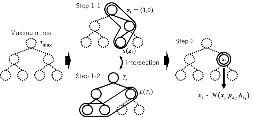
Figure 1: An overview of the data generation process.

Let $K\in\mathbb{N}$ and $D\in\mathbb{N}$ be given constants. In Step 1, a node on a $K$-ary perfect tree with depth $D$ is randomly selected. Let $T_{\mathrm{max}}$ denote the $K$-ary perfect tree. Step 1 consists of independent 2 substeps: Step 1-1 and Step 1-2. We describe each step in order.

In Step 1-1, a path from the root node to a leaf node of $T_{\mathrm{max}}$ is randomly selected in the following manner. First, we define some notations. Let $\mathcal{S}_{\mathrm{max}}$, $\mathcal{I}_{\mathrm{max}}$, and $\mathcal{L}_{\mathrm{max}}$ denote the set of all nodes, inner nodes, and leaf nodes of $T_{\mathrm{max}}$, respectively. Let $s_{\lambda}$ denote the root node of $T_{\mathrm{max}}$. The depth of any node $s\in\mathcal{S}_{\mathrm{max}}$ is denoted by $d_{s}$, e.g., $s_{\lambda}=0$. We define $\mathrm{Ch}(s)$ as a set of child node of $s$ on $T_{\mathrm{max}}$.

We assume each inner node $s\in\mathcal{I}_{\mathrm{max}}$ has a routing parameter $\bm{\pi}_{s}\coloneqq(\pi_{s,s_{\mathrm{ch}}})_{s_{\mathrm{ch}}\in\mathrm{Ch}(s)}\in\mathbb{R}^{K}$ that satisfies $\sum_{s_{\mathrm{ch}}\in\mathrm{Ch}(s)}\pi_{s,s_{\mathrm{ch}}}=1$, and we define its tuple $\bm{\pi}\coloneqq(\bm{\pi}_{s})_{s\in\mathcal{I}_{\mathrm{max}}}$. According to the routing parameter $\bm{\pi}$, a path from the root node $s_{\lambda}$ to a leaf node $s(\bm{z}_{i})$ is randomly generated in the following manner. The path is determined by a latent variable $\bm{z}\coloneqq(z_{i,1},z_{i,2},\dots,z_{i,D})^{\top}\in\{0,1,\dots,K-1\}^{D}$. First, $z_{i,1}$ is generated according to $\bm{\pi}_{s_{\lambda}}$, i.e., $z_{i,1}=k$ holds with probability $\pi_{s_{\lambda},s_{k}}$, where $s_{k}$ denotes the $k$th child node of $s_{\lambda}$. Then, $z_{i,2}$ is generated according to $\bm{\pi}_{s_{k}}$ in a similar manner. This procedure is repeated until we reach one of the leaf nodes of $T_{\mathrm{max}}$. Let $s(\bm{z}_{i})$ denote the leaf node determined by this procedure. Thus, the probability distribution of $\bm{z}_{i}$ is represented as follows.

Definition 1.

We define the probability distribution of $\bm{z}_{i}$ given $\bm{\pi}$ as follows:

$$p(\bm{z}_{i}|\bm{\pi})\coloneqq\prod_{s\in\mathcal{I}_{\mathrm{max}}}\prod_{s_{\mathrm{ch}}\in\mathrm{Ch}(s)}\pi_{s,s_{\mathrm{ch}}}^{I\{s_{\mathrm{ch}}\preceq s(\bm{z}_{i})\}},$$ (1)

where $I\{\cdot\}$ denotes the indicator function and $s_{\mathrm{ch}}\preceq s(\bm{z}_{i})$ represents $s_{\mathrm{ch}}$ is an ancestor node of $s(\bm{z}_{i})$ or equal to $s(\bm{z}_{i})$.

In Step 1-2, a latent subtree $T_{i}$ for the $i$th data point is generated according to the following procedure. Let $T_{i}$ denote a full (also called proper) subtree of $T_{\mathrm{max}}$, where $T_{i}$’s root node is $s_{\lambda}$. Each inner node of $T_{i}$ havs exactly $K$ children. Let $\mathcal{T}$ denote the set of all such subtrees of $T_{\mathrm{max}}$. The set of all nodes, inner nodes, and leaf nodes of $T_{i}$ are denoted by $\mathcal{S}(T_{i})$, $\mathcal{I}(T_{i})$, and $\mathcal{L}(T_{i})$, respectively. Then, $T_{i}$ is generated according to the following probability distribution, which is used in text compression (e.g., [1]) and mathematically summarized in [2].

Definition 2 ([2]).

$$p(T_{i}|\bm{g})\coloneqq\prod_{s\in\mathcal{I}(T_{i})}g_{s}\prod_{s^{\prime}\in\mathcal{L}(T_{i})}(1-g_{s^{\prime}}),$$ (2)

where $g_{s}\in[0,1]$ is a parameter representing an edge spreading probability of a node $s\in\mathcal{S}_{\mathrm{max}}$ and $\bm{g}$ denotes $(g_{s})_{s\in\mathcal{S}_{\mathrm{max}}}$. For $s\in\mathcal{L}_{\mathrm{max}}$, we assume $g_{s}=0$.

Remark 1.

Eq. (2) satisfies the condition of the probability distribution over $\mathcal{T}$, i.e., $\sum_{T_{i}\in\mathcal{T}}p(T_{i}|\bm{g})=1$ holds. The meaning of (2) is detailed in Fig. 2 in [2]. Other properties have also been discussed in [2].

At the end of Step 1, we take the intersection of $\mathcal{L}(T_{i})$ and the nodes on the path from $s_{\lambda}$ to $s(\bm{z}_{i})$. Then, one of the nodes in $\mathcal{S}_{\mathrm{max}}$, i.e., a node $s$ that satisfies $(s\in\mathcal{L}(T_{i}))\land(s\preceq s(\bm{z}_{i}))$, is uniquely determined. Let $s_{i}$ denote it.

In Step 2, a data point is generated and observed in the following manner. Let the dimension of the observed data be $p\in\mathbb{N}$. Let $\bm{x}_{i}=(x_{i,1},x_{i,2},\dots,x_{i,p})^{\top}\in\mathbb{R}^{p}$ denote the $i$th data point. We assume each node $s\in\mathcal{S}_{\mathrm{max}}$ has a mean vector $\bm{\mu}_{s}\in\mathbb{R}^{p}$ and a precision matrix $\bm{\Lambda}_{s}\in\mathbb{R}^{p\times p}$, which is assumed to be positive definite. We define the following tuples: $\bm{\mu}\coloneqq(\bm{\mu}_{s})_{s\in\mathcal{S}_{\mathrm{max}}}$ and $\bm{\Lambda}\coloneqq(\bm{\Lambda}_{s})_{s\in\mathcal{S}_{\mathrm{max}}}$. Given $T_{i}$, $\bm{\mu}$, $\bm{\Lambda}$, and $\bm{z}_{i}$, we assume the $i$th data point $\bm{x}_{i}$ is i.i.d. generated according to the following distribution.

Definition 3.

We define the probability density function of $\bm{x}_{i}$ given $\bm{z}_{i}$, $T_{i}$, $\bm{\mu}$, and $\bm{\Lambda}$ as follows:

$$p(\bm{x}_{i}|\bm{z}_{i},T_{i},\bm{\mu},\bm{\Lambda})\coloneqq\prod_{s\in\mathcal{L}(T_{i})}\mathcal{N}(\bm{x}_{i}|\bm{\mu}_{s},\bm{\Lambda}_{s}^{-1})^{I\{s\preceq s(\bm{z}_{i})\}},$$ (3)

where $\mathcal{N}(\cdot)$ represents the probability density function of the Gaussian distribution.

Note that this data generation process is equivalent to a truncated version of the TS-SBP in [4]. Let $s_{i}$ denote the node determined by $T_{i}$ and $\bm{z}_{i}$, i.e., $(s_{i}\in\mathcal{L}(T_{i}))\land(s_{i}\preceq s(\bm{z}_{i}))$ holds, and $S_{i}$ denote the corresponding random variable on $\mathcal{S}_{\mathrm{max}}$. Then, the following theorem holds.

Theorem 1.

The probability distribution of $S_{i}$ over $\mathcal{S}_{\mathrm{max}}$ is represented as follows.

$$\mathrm{Pr}\{S_{i}=s_{i}\}=(1-g_{s_{i}})\pi_{(s_{i})_{\mathrm{pa}},s_{i}}\prod_{s^{\prime}\prec{s_{i}}}\pi_{s^{\prime}_{\mathrm{pa}},s^{\prime}}g_{s^{\prime}},$$ (4)

where $s_{\mathrm{pa}}$ denotes the parent node of $s$ and we assume $\pi_{s_{\mathrm{pa}},s}=1$ for $s=s_{\lambda}$. The above distribution is equivalent to a truncated version of the TS-SBP, where tree width and depth are $K$ and $D$, respectively.

Proof.

:

$$\mathrm{Pr}\{S_{i}=s_{i}\}=\left(\sum_{T_{i}\in\mathcal{T}}I\{s_{i}\in\mathcal{L}(T_{i})\}p(T_{i}|\bm{g})\right)$$

$$\qquad\times\left(\sum_{\bm{z}_{i}\in\{0,1,\dots K-1\}^{D}}I\{s_{i}\preceq s(\bm{z}_{i})\}p(\bm{z}_{i}|\bm{\pi})\right)$$ (5)

$$=\left((1-g_{s_{i}})\prod_{s^{\prime}\prec{s_{i}}}g_{s^{\prime}}\right)\left(\pi_{(s_{i})_{\mathrm{pa}},s_{i}}\prod_{s^{\prime}\prec{s_{i}}}\pi_{s^{\prime}_{\mathrm{pa}},s^{\prime}}\right)$$ (6)

$$=(1-g_{s_{i}})\pi_{(s_{i})_{\mathrm{pa}},s_{i}}\prod_{s^{\prime}\prec{s_{i}}}\pi_{s^{\prime}_{\mathrm{pa}},s^{\prime}}g_{s^{\prime}}.$$ (7)

In the second equation, we used Theorem 2 of [2]. Eq. (7) is equivalent to Eq. (2) in [4] except that the tree width and depth are limited. It is because $\mathrm{Pr}\{S_{i}=s_{i}\}$, $g_{s_{i}}$, $1-g_{s_{i}}$, and $\pi_{(s_{i})_{\mathrm{pa}},s_{i}}$ correspond to $\pi_{\bm{\epsilon}}$, $1-\nu_{\bm{\epsilon}}$, $\nu_{\bm{\epsilon}}$, and $\varphi_{\bm{\epsilon}}$ in [4], respectively. $\Box$

III Variational Bayesian methods

We assume $\{\bm{x}_{i}\}_{i=1}^{n}$ is generated and observed according to the model described in the previous section. Let $\bm{x}$ denote $\{\bm{x}_{i}\}_{i=1}^{n}$. We assume a prior distribution for $\bm{\pi}$, $\bm{g}$, $\bm{\mu}$, and $\bm{\Lambda}$ and estimate the posterior distribution for $\{\bm{z}_{i}\}_{i=0}^{n}$, $\{T_{i}\}_{i=0}^{n}$, $\bm{\pi}$, $\bm{g}$, $\bm{\mu}$, $\bm{\Lambda}$ from $\bm{x}$. Hereafter, let $\bm{z}$ denote $\{\bm{z}_{i}\}_{i=0}^{n}$ and $\bm{T}$ denote $\{T_{i}\}_{i=0}^{n}$. Unfortunately, we do not have a closed form expression of the posterior distribution $p(\bm{z},\bm{T},\bm{\pi},\bm{g},\bm{\mu},\bm{\Lambda}|\bm{x})$. To approximate it, only MCMC methods have been proposed in [4], but any VB mehtods have not been proposed yet. Therefore, we propose a VB method here. To reduce the computational complexity, we impose the following assumptions on the prior distribution.

III-A Prior distributions

Assumption 1.

Given $\bm{\alpha}_{s}\in\mathbb{R}_{>0}^{K}$ for all $s\in\mathcal{I}_{\mathrm{max}}$, we assume the following probability distribution for $\bm{\pi}$, which is also known as Dirichlet tree distributions [7].

$$p(\bm{\pi})\coloneqq\prod_{s\in\mathcal{I}_{\mathrm{max}}}\mathrm{Dir}(\bm{\pi}_{s}|\bm{\alpha}_{s}),$$ (8)

where $\mathrm{Dir}(\cdot)$ denotes a probability density function of the Dirichlet distribution.

Assumption 2.

Given $a_{s}\in\mathbb{R}_{>0}$ and $b_{s}\in\mathbb{R}_{>0}$ for all $s\in\mathcal{I}_{\mathrm{max}}$, we assume the following probability distribution for $\bm{g}$, which is known as a conjugate prior of $p(T_{i}|\bm{g})$ [2].

$$p(\bm{g})\coloneqq\prod_{s\in\mathcal{I}_{\mathrm{max}}}\mathrm{Beta}(g_{s}|a_{s},b_{s}),$$ (9)

where $\mathrm{Beta}(\cdot)$ denotes a probability density function of the beta distribution. Note that $g_{s}$ for $s\in\mathcal{L}_{\mathrm{max}}$ is not a random variable but a constant equal to $0$.

Assumption 3.

Given a real number $\nu_{s}>p-1$ and a positive definite matrix $\bm{W}_{s}\in\mathbb{R}^{p\times p}$ for all $s\in\mathcal{S}_{\mathrm{max}}$, we assume the following probability distribution for $\bm{\Lambda}$.

$$p(\bm{\Lambda}) \coloneqq\prod_{s\in\mathcal{S}_{\mathrm{max}}}\mathcal{W}(\bm{\Lambda}_{s}|\nu_{s},\bm{W}_{s}),$$ (10)

where $\mathcal{W}(\cdot)$ denotes a probability density function of the Wishart distribution.

Assumption 4.

Given a real number $u>p-1$ and a positive definite matrix $\bm{V}\in\mathbb{R}^{p\times p}$, we assume the following probability distribution for $\bm{\mu}$ with an additional parameter $\bm{L}\in\mathbb{R}^{p\times p}$.

$$p(\bm{L}) \coloneqq\mathcal{W}(\bm{L}|u,\bm{V}),$$ (11)

$$p(\bm{\mu}|\bm{L}) \coloneqq\prod_{s\in\mathcal{S}_{\mathrm{max}}}\mathcal{N}(\bm{\mu}_{s}|\bm{\mu}_{s_{\mathrm{pa}}},\bm{L}^{-1}),$$ (12)

where $s_{\mathrm{pa}}$ denotes the parent node of $s$. For the root node $s_{\lambda}$, we assume $\bm{\mu}_{(s_{\lambda})_{\mathrm{pa}}}\coloneqq\bm{m}_{s_{\lambda}}$ is given as a hyperparameter.

By Assumption 4, mixture components whose means are close to each other tend to be descendant nodes of a common node.

III-B Overview of variational Bayesian methods

In the VB method, the posterior distribution $p(\bm{z},\bm{T},\bm{\pi},$ $\bm{g},\bm{\mu},\bm{\Lambda},\bm{L}|\bm{x})$ is approximated by a distribution $q(\bm{z},\bm{T},\bm{\pi},$ $\bm{g},\bm{\mu},\bm{\Lambda},\bm{L})$ called variational distribution (see, e.g., [6]). We assume our variational distribution fulfills the following factorization property.

Assumption 5.

We assume the following factorization.

$$q(\bm{z},\bm{T},\bm{\pi},\bm{g},\bm{\mu},\bm{\Lambda},\bm{L})=q(\bm{g})q(\bm{L})\prod_{i=1}^{n}q(\bm{z}_{i})\prod_{i=1}^{n}q(T_{i})$$

$$\qquad\times\prod_{s\in\mathcal{I}_{\mathrm{max}}}q(\bm{\pi}_{s})\prod_{s\in\mathcal{S}_{\mathrm{max}}}q(\bm{\mu}_{s})\prod_{s\in\mathcal{S}_{\mathrm{max}}}q(\bm{\Lambda}_{s}).$$ (13)

It is known (see, e.g., [6]) that minimizing the Kullback-Leibler divergence $\mathrm{KL}(q(\bm{z},\bm{T},\bm{\pi},\bm{g},\bm{\mu},\bm{\Lambda},\bm{L})||p(\bm{z},\bm{T},\bm{\pi},\bm{g},$ $\bm{\mu},\bm{\Lambda},\bm{L}|\bm{x}))$ is equivalent to maximizing the variational lower bound. Further, it is also known (see, e.g., [6]) that the optimal variational distribution that maximizes the variational lower bound fulfills

$$\ln q^{*}(\bm{z}_{i})\!=\!\mathbb{E}_{\backslash\bm{z}_{i}}\left[\ln p(\bm{x},\bm{z},\bm{T},\bm{\pi},\bm{g},\bm{\mu},\bm{\Lambda},\bm{L})\right]\!+\!\mathrm{const.},$$ (14)

$$\ln q^{*}(T_{i})\!=\!\mathbb{E}_{\backslash T_{i}}\left[\ln p(\bm{x},\bm{z},\bm{T},\bm{\pi},\bm{g},\bm{\mu},\bm{\Lambda},\bm{L})\right]\!+\!\mathrm{const.},$$ (15)

$$\ln q^{*}(\bm{\pi}_{s})\!=\!\mathbb{E}_{\backslash\bm{\pi}_{s}}\left[\ln p(\bm{x},\bm{z},\bm{T},\bm{\pi},\bm{g},\bm{\mu},\bm{\Lambda},\bm{L})\right]\!+\!\mathrm{const.},$$ (16)

$$\ln q^{*}(\bm{g})\!=\!\mathbb{E}_{\backslash\bm{g}}\left[\ln p(\bm{x},\bm{z},\bm{T},\bm{\pi},\bm{g},\bm{\mu},\bm{\Lambda},\bm{L})\right]\!+\!\mathrm{const.},$$ (17)

$$\ln q^{*}(\bm{\mu}_{s})\!=\!\mathbb{E}_{\backslash\bm{\mu}_{s}}\!\left[\ln p(\bm{x},\bm{z},\bm{T},\bm{\pi},\bm{g},\bm{\mu},\bm{\Lambda},\bm{L})\right]\!+\!\mathrm{const.},$$ (18)

$$\ln q^{*}(\bm{\Lambda}_{s})\!=\!\mathbb{E}_{\backslash\bm{\Lambda}_{s}}\!\left[\ln p(\bm{x},\bm{z},\bm{T},\bm{\pi},\bm{g},\bm{\mu},\bm{\Lambda},\bm{L})\right]\!+\!\mathrm{const.},\!$$ (19)

$$\ln q^{*}(\bm{L})\!=\!\mathbb{E}_{\backslash\bm{L}}\left[\ln p(\bm{x},\bm{z},\bm{T},\bm{\pi},\bm{g},\bm{\mu},\bm{\Lambda},\bm{L})\right]\!+\!\mathrm{const.}$$ (20)

where $\mathbb{E}_{\backslash(\star)}$ means the expectation for all the latent variables except $(\star)$.

However, $q^{*}(\bm{z}_{i})$, $q^{*}(T_{i})$, $q^{*}(\bm{\pi}_{s})$, $q^{*}(\bm{g})$, $q^{*}(\bm{\mu}_{s})$, $q^{*}(\bm{\Lambda}_{s})$ and $q^{*}(\bm{L})$ depend on each other. Therefore, we update them in turn from an initial value until the convergence by using Eqs. (14) to (20) as updating formulas.

III-C Update of $q(\bm{\pi}_{s})$, $q(\bm{\mu}_{s})$, $q(\bm{\Lambda}_{s})$, $q(\bm{L})$, $q(\bm{g})$, and $q(\bm{z}_{i})$

For $\bm{\pi}_{s}$, $\bm{\mu}_{s}$, $\bm{\Lambda}_{s}$, $\bm{L}$, $\bm{g}$, and $\bm{z}_{i}$, we assumed locally conjugate prior distributions. Therefore, $q(\bm{\pi}_{s})$, $q(\bm{\mu}_{s})$, $q(\bm{\Lambda}_{s})$, $q(\bm{L})$, $q(\bm{g})$, and $q(\bm{z}_{i})$ have the same form as the prior distributions.

Proposition 1.

There exist parameters $\hat{\bm{\alpha}}_{s}\in\mathbb{R}_{>0}^{K}$, $\hat{\bm{m}}_{s}\in\mathbb{R}^{p}$, $\hat{\bm{L}}_{s}\in\mathbb{R}^{p\times p}$, $\hat{\nu}_{s}\in\mathbb{R}$, $\hat{\bm{W}}_{s}\in\mathbb{R}^{p\times p}$, $\hat{u}\in\mathbb{R}$, $\hat{\bm{V}}\in\mathbb{R}^{p\times p}$, $\hat{a}_{s}\in\mathbb{R}_{>0}$, $\hat{b}_{s}\in\mathbb{R}_{>0}$, and $\hat{\pi}_{i,s,s_{\mathrm{ch}}}\in\mathbb{R}_{>0}$ such that $q(\bm{\pi}_{s})$, $q(\bm{\mu}_{s})$, $q(\bm{\Lambda}_{s})$, $q(\bm{L})$, $q(\bm{g})$, and $q(\bm{z}_{i})$ have the following representation.

$$q(\bm{\pi}_{s}) =\mathrm{Dir}(\bm{\pi}_{s}|\hat{\bm{\alpha}}_{s}),$$ (21)

$$q(\bm{\mu}_{s}) =\mathcal{N}(\bm{\mu}_{s}|\hat{\bm{m}}_{s},\hat{\bm{L}}_{s}^{-1}),$$ (22)

$$q(\bm{\Lambda}_{s}) =\mathcal{W}(\bm{\Lambda}_{s}|\hat{\nu}_{s},\hat{\bm{W}}_{s}),$$ (23)

$$q(\bm{L}) =\mathcal{W}(\bm{L}|\hat{u},\hat{\bm{V}}),$$ (24)

$$q(\bm{g}) =\prod_{s\in\mathcal{I}_{\mathrm{max}}}\mathrm{Beta}(g_{s}|\hat{a}_{s},\hat{b}_{s}),$$ (25)

$$q(\bm{z}_{i}) =\prod_{s\in\mathcal{I}_{\mathrm{max}}}\prod_{s_{\mathrm{ch}}\in\mathrm{Ch}(s)}\hat{\pi}_{i,s,s_{\mathrm{ch}}}^{I\{s_{\mathrm{ch}}\preceq s(\bm{z}_{i})\}}.$$ (26)

This proposition is almost straightforwardly proved by using basic theorems in Bayesian statistics and theorems in [2]. The proof and specific updating formulas of the parameters are detailed in Appendix A.

Based on Proposition 1, we define some quantities in advance. First, for any $s$, let $q(s\preceq s(\bm{z}_{i}))$ denote the probability that the event $\{\bm{z}_{i}\mid s\preceq s(\bm{z}_{i})\}$ occurs under $q(\bm{z}_{i})$, i.e.,

$$q(s\preceq s(\bm{z}_{i}))\coloneqq \mathbb{E}_{q(\bm{z}_{i})}[I\{s\preceq s(\bm{z}_{i})\}]$$ (27)

$$= \prod_{s^{\prime}\preceq s}\hat{\pi}_{i,s^{\prime}_{\mathrm{pa}},s^{\prime}}.$$ (28)

In addition, we define the following quantities.

$$\ln\phi_{i,s} \coloneqq q(s\preceq s(\bm{z}_{i}))\mathbb{E}_{q(\bm{\mu}_{s},\bm{\Lambda}_{s})}[\ln\mathcal{N}(\bm{x}_{i}|\bm{\mu}_{s},\bm{\Lambda}_{s}^{-1})],$$ (29)

$$\ln\tilde{g}_{s} \coloneqq\mathbb{E}_{q(g_{s})}[\ln g_{s}],$$ (30)

$$\ln\tilde{g}_{s}^{c} \coloneqq\mathbb{E}_{q(g_{s})}[\ln(1-g_{s})].$$ (31)

III-D Update of $q(T_{i})$

First, we briefly review the difficulty in calculating the variational distribution for $T_{i}$. Generally speaking, even if the prior distribution $p(T_{i})$ had a parametric form, variational distribution $q(T_{i})$ does not necessarily have the same form. Trivially, we can represent $q(T_{i})$ by memorizing all the probabilities of the trees in $\mathcal{T}$. However, this representation requires $|\mathcal{T}|$ number of parameters, which is doubly exponential to the depth of trees, and computationally expensive.

To solve this difficulty, we derive the same parametric representation of $q(T_{i})$ as the prior distribution $p(T_{i})$ by applying the Bayes coding algorithm for context tree sources[1]. This representation requires only $|\mathcal{S}_{\mathrm{max}}|$ number of parameters. Moreover, the updating formula of these parameters is locally optimal when we fix the variational distributions other than $q(T_{i})$, i.e., we can calculate the expectation in (15) without any approximation.

Theorem 2.

The updating formula for $q(T_{i})$ is given as follows:

$$q(T_{i})=\prod_{s\in\mathcal{I}(T_{i})}\hat{g}_{i,s}\prod_{s^{\prime}\in\mathcal{L}(T_{i})}(1-\hat{g}_{i,s^{\prime}}),$$ (32)

where $\hat{g}_{i,s}\in[0,1]$ is obtained as follows:

$$\hat{g}_{i,s}\coloneqq\begin{cases}\frac{\tilde{g}_{s}\prod_{s_{\mathrm{ch}}\in\mathrm{Ch}(s)}\rho_{i,s_{\mathrm{ch}}}}{\rho_{i,s}},&s\in\mathcal{I}_{\mathrm{max}},\\ 0,&s\in\mathcal{L}_{\mathrm{max}}.\end{cases}$$ (33)

Here, $\rho_{i,s}$ is recursively defined in the following manner.

$$\rho_{i,s}\!\coloneqq\!\begin{cases}\tilde{g}_{s}^{c}\phi_{i,s}+\tilde{g}_{s}\prod_{s_{\mathrm{ch}}\in\mathrm{Ch}(s)}\rho_{i,s_{\mathrm{ch}}},\!&s\in\mathcal{I}_{\mathrm{max}},\\ \phi_{i,s},&s\in\mathcal{L}_{\mathrm{max}}.\end{cases}$$ (34)

The proof of this theorem is in Appendix B. It should be noted that Eqs. (33) and (34) correspond to the Bayes coding algorithm for context tree sources, e.g., Eqs. (12) and (9) in [1], respectively.

III-E Initialization

In this paper, we use the following initialization of the variational distribution. We initialize the parameters of $q(\bm{T},\bm{\pi},\bm{g},\bm{\mu},\bm{\Lambda},\bm{L})$ and start updating from $q(\bm{z})$. First, we deterministically initialize the parameters other than $\hat{\bm{m}}_{s}$ for any node $s$ and its child node $s_{\mathrm{ch}}$ as follows: $\hat{u}=u$, $\hat{\bm{V}}=\bm{V}$ $\hat{a}_{s}=a_{s}$, $\hat{b}_{s}=b_{s}$, $\hat{g}_{s}=\frac{a_{s}}{a_{s}+b_{s}}$, $\hat{\alpha}_{s,s_{\mathrm{ch}}}=\alpha_{s,s_{\mathrm{ch}}}$, $\hat{\bm{L}}_{s}=u\bm{V}$, $\hat{\nu}_{s}=\nu_{s}$, and $\hat{\bm{W}}_{s}=\bm{W}_{s}$. Next, $\hat{\bm{m}}_{s}$ is randomly and recursively assigned from the root node as follows:

$$\hat{\bm{m}}_{s_{\lambda}} =\frac{1}{n}\sum_{i=1}^{n}\bm{x}_{i},$$ (35)

$$\hat{\bm{m}}_{s} \sim\mathcal{N}(\hat{\bm{m}}_{s}|\hat{\bm{m}}_{s_{\mathrm{pa}}},(u\bm{V})^{-1}).$$ (36)

Therefore, the mean $\hat{\bm{m}}_{s}$ of each node $s$ is centered on the parent’s mean $\hat{\bm{m}}_{s_{\mathrm{pa}}}$.

IV Experiments

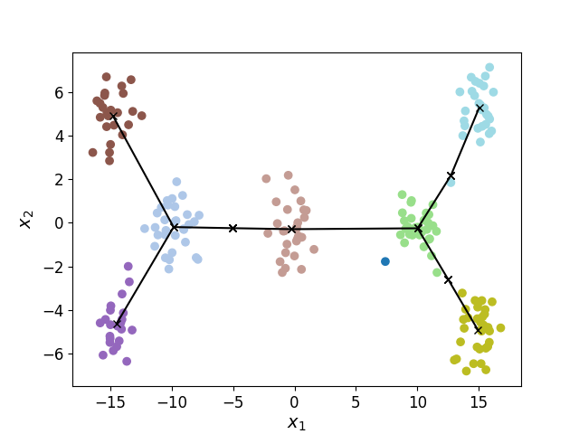
Figure 2: The input data and the estimated tree structure of the means of the mixture components.

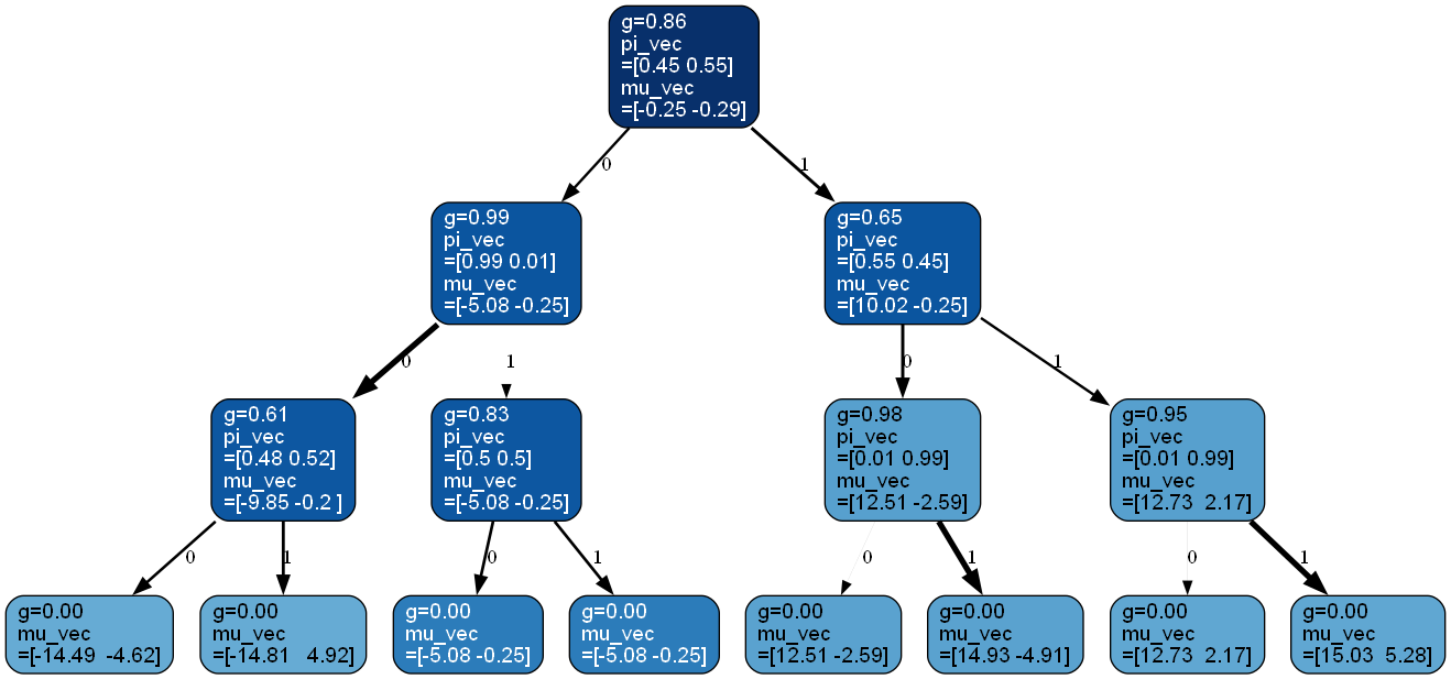
Figure 3: The TS-SBP mixture of Gaussians estimated from the data shown in Fig. 2.

In this section, we show an experimental result on synthetic data. The data are generated from a Gaussian mixture model. The means of mixture components are $[-15,-5]^{\top}$, $[-15,5]^{\top}$, $[-10,0]^{\top}$, $[0,0]^{\top}$, $[10,0]^{\top}$, $[15,-5]^{\top}$, and $[15,5]^{\top}$, and the covariance matrices are all the identity matrix $\bm{I}$. The mixing probability is uniform. Figure 2 shows the scatter plots of the generated data. The sample size is 200.

The constants of the TS-SBP mixture of Gaussians are assumed to be $p=2$, $K=2$, and $D=3$. Therefore, we have at most $15$ mixture components. We set the hyperparemeters as follows: $a_{s}=3$, $b_{s}=1$, $\alpha_{s,s_{\mathrm{ch}}}=1/2$, $\bm{m}_{s_{\lambda}}=[0,0]^{\top}$, $u=5$, $\bm{V}=\bm{I}/10$, $\nu_{s}=2$, and $\bm{W}_{s}=\bm{I}/5$ for any $s$ and $s_{\mathrm{ch}}$. The maximum number of iterations is assumed to be 400. Initial values of variational distributions are randomly generated 100 times by the procedure in the previous section. The variational distribution that shows the largest variational lower bound is used for parameter estimation.

Figures 2 and 3 show the estimated model. In Fig. 2, the dot by ’$\times$’ represents $\hat{\bm{m}}_{s}$ for each node $s$. The plot color means the MAP node for each data point. All the parameters are estimated by the expectations of the variational distributions. As shown in Fig. 2, mixture components close to each other tend to be children of a common inner node as expected.

V Conclusion

In this paper, we first re-defined the TS-SBP mixture of Gaussians by using a tree distribution summarized in [2]. Then, applying the Bayes coding algorithm for context sources[1], we derived a VB method for the TS-SBP mixture of Gaussians, while any VB methods for the TS-SBP mixture models had not been proposed previously. The derived VB method had a subroutine similar to the Bayes coding algorithm for context tree sources. We also confirmed its behavior by a numerical experiment on a toy example. As a result, our method successfully captured the hierarchical structure of the synthetic data, i.e., mixture components close to each other tend to be children of a common inner node.

Appendix A Proof of Proposition 1

In tho following, we divide Proposition 1 into six propositions for each of $q(\bm{\pi}_{s})$, $q(\bm{\mu}_{s})$, $q(\bm{\Lambda}_{s})$, $q(\bm{L})$, $q(\bm{g})$, and $q(\bm{z}_{i})$ and prove them in order.

A-1 Update of $q(\bm{\pi}_{s})$

First, we define the following notation.

$$N_{s}\coloneqq\sum_{i=1}^{n}q(s\preceq s(\bm{z}_{i})),$$ (37)

where $q(s\preceq s(\bm{z}_{i}))$ is defined in (27). Then, the following proposition holds.

Proposition 2.

The updating formula for $q(\bm{\pi}_{s})$ is given as $q(\bm{\pi}_{s})=\mathrm{Dir}(\bm{\pi}_{s}|\hat{\bm{\alpha}}_{s})$, where each element of $\hat{\bm{\alpha}}_{s}\in\mathbb{R}_{>0}^{K}$ is obtained as follows:

$$\hat{\alpha}_{s,s_{\mathrm{ch}}}\coloneqq\alpha_{s,s_{\mathrm{ch}}}+N_{s_{\mathrm{ch}}}.$$ (38)

Proof.

Calculating (16), we obtain the following equation.

$$\ln q(\bm{\pi}_{s}) =\sum_{s_{\mathrm{ch}}\in\mathrm{Ch}(s)}\left(\sum_{i=1}^{n}q(s_{\mathrm{ch}}\preceq s(\bm{z}_{i}))\right)\ln\pi_{s,s_{\mathrm{ch}}}$$

$$\quad+\ln\mathrm{Dir}(\bm{\pi}_{s}|\bm{\alpha}_{s})+\mathrm{const.},$$ (39)

Therefore, Proposition 2 holds. $\Box$

A-A Update of $q(\bm{\mu}_{s})$

First, for any $s$, let $q(s\in\mathcal{L}(T_{i}))$ denote the probability that the event $\{T_{i}\mid s\in\mathcal{L}(T_{i})\}$ occurs under $q(T_{i})$, i.e.,

$$q(s\in\mathcal{L}(T_{i}))\coloneqq\mathbb{E}_{q(T_{i})}[I\{s\in\mathcal{L}(T_{i})\}].$$ (40)

Next, we define the following notations.

$$\tilde{N}_{s} \coloneqq\sum_{i=1}^{n}q(s\in\mathcal{L}(T_{i}))q(s\preceq s(\bm{z}_{i})),$$ (41)

$$\bar{\bm{x}}_{s} \coloneqq\frac{1}{\tilde{N}_{s}}\sum_{i=1}^{n}q(s\in\mathcal{L}(T_{i}))q(s\preceq s(\bm{z}_{i}))\bm{x}_{i}.$$ (42)

Then, the following proposition holds.

Proposition 3.

The updating formula for $q(\bm{\mu}_{s})$ is given as $q(\bm{\mu}_{s})=\mathcal{N}(\bm{\mu}_{s}|\hat{\bm{m}}_{s},\hat{\bm{L}}_{s}^{-1})$, where $\hat{\bm{m}}_{s}\in\mathbb{R}^{p}$ and $\hat{\bm{L}}_{s}\in\mathbb{R}^{p\times p}$ are obtained as follows:

$$\hat{\bm{L}}_{s}\coloneqq \begin{cases}\tilde{N}_{s}\mathbb{E}_{q(\bm{\Lambda}_{s})}[\bm{\Lambda}_{s}]+(K+1)\mathbb{E}_{q(\bm{L})}[\bm{L}],&s\in\mathcal{I}_{\mathrm{max}},\\ \tilde{N}_{s}\mathbb{E}_{q(\bm{\Lambda}_{s})}[\bm{\Lambda}_{s}]+\mathbb{E}_{q(\bm{L})}[\bm{L}],&s\in\mathcal{L}_{\mathrm{max}},\end{cases}$$ (43)

$$\hat{\bm{m}}_{s}\coloneqq \begin{cases}\hat{\bm{L}}_{s}^{-1}\bigl{\{}\tilde{N}_{s}\mathbb{E}_{q(\bm{\Lambda}_{s})}[\bm{\Lambda}_{s}]\bar{\bm{x}}_{s}+\mathbb{E}_{q(\bm{L})}[\bm{L}]\\ \qquad\quad\times(\hat{\bm{m}}_{s_{\mathrm{pa}}}+\sum_{s_{\mathrm{ch\in\mathrm{Ch}(s)}}}\hat{\bm{m}}_{s_{\mathrm{ch}}})\bigr{\}},&s\in\mathcal{I}_{\mathrm{max}},\\ \hat{\bm{L}}_{s}^{-1}\bigl{\{}\tilde{N}_{s}\mathbb{E}_{q(\bm{\Lambda}_{s})}[\bm{\Lambda}_{s}]\bar{\bm{x}}_{s}\\ \qquad\quad+\mathbb{E}_{q(\bm{L})}[\bm{L}]\hat{\bm{m}}_{s_{\mathrm{pa}}}\bigr{\}},&s\in\mathcal{L}_{\mathrm{max}}.\end{cases}$$ (44)

Proof.

We prove Proposition 3 only for $s\in\mathcal{I}_{\mathrm{max}}$ because those for $s\in\mathcal{L}_{\mathrm{max}}$ will be proved similarly. Calculating (18), we obtain the following equation.

$$\ln q(\bm{\mu}_{s})$$

$$=\sum_{i=1}^{n}\mathbb{E}_{q(T_{i})}\Biggl{[}\sum_{s\in\mathcal{L}(T_{i})}q(s\preceq s(\bm{z}_{i}))$$

$$\qquad\qquad\qquad\qquad\quad\times\mathbb{E}_{q(\bm{\Lambda}_{s})}[\ln\mathcal{N}(\bm{x}_{i}|\bm{\mu}_{s},\bm{\Lambda}_{s}^{-1})]\Biggr{]}$$

$$\quad+\mathbb{E}_{q(\bm{\mu}_{s_{\mathrm{pa}}},\bm{L})}[\ln\mathcal{N}(\bm{\mu}_{s}|\bm{\mu}_{s_{\mathrm{pa}}},\bm{L}^{-1})]$$

$$\quad+\sum_{s_{\mathrm{ch}}\in\mathrm{Ch}(s)}\mathbb{E}_{q(\bm{\mu}_{s_{\mathrm{ch}}},\bm{L})}[\ln\mathcal{N}(\bm{\mu}_{s_{\mathrm{ch}}}|\bm{\mu}_{s},\bm{L}^{-1})]+\mathrm{const.}$$ (45)

Here, we can calculate the expectation for $q(T_{i})$ as follows:

$$\mathbb{E}_{q(T_{i})}\left[\sum_{s\in\mathcal{L}(T_{i})}q(s\preceq s(\bm{z}_{i}))\mathbb{E}_{q(\bm{\Lambda}_{s})}[\ln\mathcal{N}(\bm{x}_{i}|\bm{\mu}_{s},\bm{\Lambda}_{s}^{-1})]\right]$$

$$=\mathbb{E}_{q(T_{i})}\Biggl{[}\sum_{s\in\mathcal{S}_{\mathrm{max}}}I\{s\in\mathcal{L}(T_{i})\}q(s\preceq s(\bm{z}_{i}))$$

$$\qquad\qquad\qquad\qquad\quad\times\mathbb{E}_{q(\bm{\Lambda}_{s})}[\ln\mathcal{N}(\bm{x}_{i}|\bm{\mu}_{s},\bm{\Lambda}_{s}^{-1})]\Biggr{]}$$ (46)

$$=\sum_{s\in\mathcal{S}_{\mathrm{max}}}\mathbb{E}_{q(T_{i})}[I\{s\in\mathcal{L}(T_{i})\}]q(s\preceq s(\bm{z}_{i}))$$

$$\qquad\qquad\qquad\qquad\quad\times\mathbb{E}_{q(\bm{\Lambda}_{s})}[\ln\mathcal{N}(\bm{x}_{i}|\bm{\mu}_{s},\bm{\Lambda}_{s}^{-1})].$$ (47)

This technique is often used in the proof of Proposition 1. Note that $q(s\in\mathcal{L}(T_{i}))$ was defined by $\mathbb{E}_{q(T_{i})}[I\{s\in\mathcal{L}(T_{i})\}]$.

After this, we can prove Proposition 3 in a similar manner to the proof of the conjugate property of Gaussian distributions for Gaussian likelihoods with given covariance matrices. $\Box$

A-B Update of $q(\bm{\Lambda}_{s})$

First, we define the following notation.

$$\bm{S}_{s}\coloneqq\frac{1}{\tilde{N}_{s}}\sum_{i=1}^{n}q(s\in\mathcal{L}(T_{i}))q(s\preceq s(\bm{z}_{i}))$$

$$\qquad\qquad\qquad\quad\times(\bm{x}_{i}-\hat{\bm{m}}_{s})(\bm{x}_{i}-\hat{\bm{m}}_{s})^{\top}.$$ (48)

Then, the following proposition holds.

Proposition 4.

The updating formula for $q(\bm{\Lambda}_{s})$ is given as $q(\bm{\Lambda}_{s})=\mathcal{W}(\bm{\Lambda}_{s}|\hat{\nu}_{s},\hat{\bm{W}}_{s})$, where $\hat{\nu}_{s}\in\mathbb{R}$ and $\hat{\bm{W}}_{s}\in\mathbb{R}^{p\times p}$ are obtained as follows:

$$\hat{\nu}_{s} \coloneqq\nu_{s}+\tilde{N}_{s},$$ (49)

$$\hat{\bm{W}}_{s}^{-1} \coloneqq\bm{W}_{s}^{-1}+\tilde{N}_{s}(\bm{S}_{s}+\hat{\bm{L}}_{s}^{-1}).$$ (50)

Proof.

In a similar manner to (46) and (47), we transform (19) as follows.

$$\ln q(\bm{\Lambda}_{s})= \sum_{i=1}^{n}\mathbb{E}_{q(T_{i})}[I\{s\in\mathcal{L}(T_{i})\}]q(s\preceq s(\bm{z}_{i}))$$

$$\qquad\times\mathbb{E}_{q(\bm{\mu}_{s})}[\ln\mathcal{N}(\bm{x}_{i}|\bm{\mu}_{s},\bm{\Lambda}_{s}^{-1})]$$

$$+\ln\mathcal{W}(\bm{\Lambda}_{s}|\nu_{s},\bm{W}_{s})+\mathrm{const.}$$ (51)

Then, in a similar manner to the proof of the conjugate property of Wishart distributions for Gaussian likelihoods with given means, Proposition 4 holds. $\Box$

A-C Update of $q(\bm{L})$

Proposition 5.

The updating formula for $q(\bm{L})$ is given as $q(\bm{L})=\mathcal{W}(\bm{L}|\hat{u},\hat{\bm{V}})$, where $\hat{u}\in\mathbb{R}$ and $\hat{\bm{V}}\in\mathbb{R}^{p\times p}$ are obtained as follows:

$$\hat{u} \coloneqq u+|\mathcal{S}_{\mathrm{max}}|,$$ (52)

$$\hat{\bm{V}}^{-1} \coloneqq\bm{V}^{-1}+\hat{\bm{L}}_{s_{\lambda}}^{-1}+(\hat{\bm{m}}_{s_{\lambda}}-\bm{m}_{s_{\lambda}})(\hat{\bm{m}}_{s_{\lambda}}-\bm{m}_{s_{\lambda}})^{\top},$$

$$\qquad+\sum_{s\in\mathcal{S}_{\mathrm{max}}\backslash\{s_{\lambda}\}}\Bigl{(}\hat{\bm{L}}_{s}^{-1}+\hat{\bm{L}}_{s_{\mathrm{pa}}}^{-1}$$

$$\qquad\qquad\quad+(\hat{\bm{m}}_{s_{\lambda}}-\hat{\bm{m}}_{s_{\mathrm{pa}}})(\hat{\bm{m}}_{s_{\lambda}}-\hat{\bm{m}}_{s_{\mathrm{pa}}})^{\top}\Bigr{)},$$ (53)

where $|\cdot|$ represents the number of elements in a set, i.e., $|\mathcal{S}_{\mathrm{max}}|$ means the total number of the nodes in $T_{\mathrm{max}}$.

Proof.

Calculating (20), we obtain the following equation.

$$\ln q(\bm{L}) =\mathbb{E}_{q(\bm{\mu}_{s_{\lambda}})}[\ln\mathcal{N}(\bm{\mu}_{s_{\lambda}}|\bm{m}_{s_{\lambda}},\bm{L}^{-1})]$$

$$\quad+\sum_{s\in\mathcal{S}_{\mathrm{max}}\setminus\{s_{\lambda}\}}\mathbb{E}_{q(\bm{\mu}_{s},\bm{\mu}_{s_{\mathrm{pa}}})}[\ln\mathcal{N}(\bm{\mu}_{s}|\bm{\mu}_{s_{\mathrm{pa}}},\bm{L}^{-1})]$$

$$\quad+\ln\mathcal{W}(\bm{L}|u,\bm{V})+\mathrm{const}.$$ (54)

Then, in a similar manner to the proof of the conjugate property of Wishart distributions for Gaussian likelihoods with given means, Proposition 5 holds. $\Box$

A-D Update of $q(\bm{g})$

First, for any $s$, let $q(s\in\mathcal{I}(T_{i}))$ denote the probability that the event $\{T_{i}\mid s\in\mathcal{I}(T_{i})\}$ occurs under $q(T_{i})$ in a similar manner to $q(s\in\mathcal{L}(T_{i}))$, i.e.,

$$q(s\in\mathcal{I}(T_{i}))\coloneqq\mathbb{E}_{q(T_{i})}[I\{s\in\mathcal{I}(T_{i})\}].$$ (55)

Then, the following proposition holds.

Proposition 6.

The updating formula for $q(\bm{g})$ is given as $q(\bm{g})=\prod_{s\in\mathcal{I}_{\mathrm{max}}}\mathrm{Beta}(g_{s}|\hat{a}_{s},\hat{b}_{s})$, where $\hat{a}_{s}\in\mathbb{R}_{>0}$ and $\hat{b}_{s}\in\mathbb{R}_{>0}$ are obtained as follows:

$$\hat{a}_{s} \coloneqq a_{s}+\sum_{i=1}^{n}q(s\in\mathcal{I}(T_{i})),$$ (56)

$$\hat{b}_{s} \coloneqq b_{s}+\sum_{i=1}^{n}q(s\in\mathcal{L}(T_{i})).$$ (57)

Proof.

Calculating (17), we obtain the following equation.

$$\ln q(\bm{g})$$

$$=\sum_{i=1}^{n}\mathbb{E}_{q(T_{i})}\left[\sum_{s\in\mathcal{I}(T_{i})}\ln g_{s}+\sum_{s\in\mathcal{L}(T_{i})\setminus\mathcal{L}_{\mathrm{max}}}\ln(1-g_{s})\right]$$

$$\qquad+\sum_{s\in\mathcal{I}_{\mathrm{max}}}\ln\mathrm{Beta}(g_{s}|a_{s},b_{s})+\mathrm{const.}$$ (58)

$$=\sum_{s\in\mathcal{I}_{\mathrm{max}}}\Biggl{\{}\left(\sum_{i=1}^{n}\mathbb{E}_{q(T_{i})}[I\{s\in\mathcal{I}(T_{i})]\right)\ln g_{s}$$

$$\qquad\qquad\quad+\left(\sum_{i=1}^{n}\mathbb{E}_{q(T_{i})}[I\{s\in\mathcal{L}(T_{i})]\right)\ln(1-g_{s})$$

$$\qquad\qquad\quad+\ln\mathrm{Beta}(g_{s}|a_{s},b_{s})\Biggr{\}}+\mathrm{const.}$$ (59)

Here, we used a technique similar to that used in (46) and (47). Note that $q(s\in\mathcal{I}(T_{i}))$ and $q(s\in\mathcal{L}(T_{i}))$ were defined by $\mathbb{E}_{q(T_{i})}[I\{s\in\mathcal{I}(T_{i})\}]$ and $\mathbb{E}_{q(T_{i})}[I\{s\in\mathcal{L}(T_{i})\}]$, respectively. Then, in a similar manner to the conjugate property of beta distributions for likelihoods of Bernoulli distributions, Proposition 6 holds. $\Box$

A-E Update of $q(\bm{z}_{i})$

Proposition 7.

The updating formula for $q(\bm{z}_{i})$ is as follows:

$$q(\bm{z}_{i})=\prod_{s\in\mathcal{I}_{\mathrm{max}}}\prod_{s_{\mathrm{ch}}\in\mathrm{Ch}(s)}\hat{\pi}_{i,s,s_{\mathrm{ch}}}^{I\{s_{\mathrm{ch}}\preceq s(\bm{z}_{i})\}},$$ (60)

where $\hat{\pi}_{i,s,s_{\mathrm{ch}}}\in\mathbb{R}_{>0}$ is defined as

$$\hat{\pi}_{i,s,s_{\mathrm{ch}}}\coloneqq\frac{\xi_{i,s,s_{\mathrm{ch}}}}{\sum_{s_{\mathrm{ch}}\in\mathrm{Ch}(s)}\xi_{i,s,s_{\mathrm{ch}}}},$$ (61)

and $\xi_{i,s,s_{\mathrm{ch}}}\in\mathbb{R}_{>0}$ is recursively defined as follows:

$$\ln\xi_{i,s,s_{\mathrm{ch}}}\coloneqq\begin{cases}\mathbb{E}_{q(\bm{\pi}_{s})}[\ln\pi_{s,s_{\mathrm{ch}}}]+\ln\zeta_{i,s_{\mathrm{ch}}}\\ \quad+\ln\sum_{s^{\prime}\in\mathrm{Ch}(s_{\mathrm{ch}})}\xi_{i,s_{\mathrm{ch}},s^{\prime}},&s_{\mathrm{ch}}\in\mathcal{I}_{\mathrm{max}},\\ \mathbb{E}_{q(\bm{\pi}_{s})}[\ln\pi_{s,s_{\mathrm{ch}}}]+\ln\zeta_{i,s_{\mathrm{ch}}},&s_{\mathrm{ch}}\in\mathcal{L}_{\mathrm{max}}.\end{cases}$$ (62)

Here, $\zeta_{i,s}$ is defined as follows:

$$\ln\zeta_{i,s}\coloneqq q(s\in\mathcal{L}(T_{i}))\mathbb{E}_{q(\bm{\mu}_{s},\bm{\Lambda}_{s})}[\ln\mathcal{N}(\bm{x}_{i}|\bm{\mu}_{s},\bm{\Lambda}_{s}^{-1})]$$ (63)

Proof.

In a similar manner to (46) and (47), we transform (14) as follows.

$$\ln q(\bm{z}_{i})$$

$$=\sum_{s\in\mathcal{S}_{\mathrm{max}}}\mathbb{E}_{q(T_{i})}[I\{s\in\mathcal{L}(T_{i})\}]I\{s\preceq s(\bm{z}_{i})\}$$

$$\qquad\qquad\quad\times\mathbb{E}_{q(\bm{\mu}_{s},\bm{\Lambda}_{s})}[\ln\mathcal{N}(\bm{x}_{i}|\bm{\mu}_{s},\bm{\Lambda}_{s}^{-1})]$$

$$\quad\!+\!\sum_{s\in\mathcal{I}_{\mathrm{max}}}\sum_{s_{\mathrm{ch}}\in\mathrm{Ch}(s)}\!I\{s_{\mathrm{ch}}\preceq s(\bm{z}_{i})\}\mathbb{E}_{q(\bm{\pi}_{s})}[\ln\pi_{s,s_{\mathrm{ch}}}]+\mathrm{const.}$$ (64)

$$=\ln\zeta_{i,s_{\lambda}}+\sum_{s\in\mathcal{I}_{\mathrm{max}}}\sum_{s_{\mathrm{ch}}\in\mathrm{Ch}(s)}I\{s_{\mathrm{ch}}\preceq s(\bm{z}_{i})\}$$

$$\qquad\qquad\qquad\quad\times(\mathbb{E}_{q(\bm{\pi}_{s})}[\ln\pi_{s,s_{\mathrm{ch}}}]+\ln\zeta_{i,s_{\mathrm{ch}}})+\mathrm{const.},$$ (65)

where $\ln\zeta_{i,s}$ is defined in (63). Note that the first term of (65) is independent of $\bm{z}_{i}$.

Next, we substitute the definitions of $\hat{\pi}_{i,s,s_{\mathrm{ch}}}$ and $\xi_{i,s,s_{\mathrm{ch}}}$ into the logarithm of (60) and bring it back to (65). First, we show another representation of the logarithm of the right-hand side of (60) with the notation $s_{\mathrm{pa}}$ that represents the parent node of $s$.

$$\sum_{s\in\mathcal{I}_{\mathrm{max}}}\sum_{s_{\mathrm{ch}}\in\mathrm{Ch}(s)}I\{s_{\mathrm{ch}}\preceq s(\bm{z}_{i})\}\ln\hat{\pi}_{i,s,s_{\mathrm{ch}}}$$

$$=\sum_{s\in\mathcal{I}_{\mathrm{max}}\setminus\{s_{\lambda}\}}I\{s\preceq s(\bm{z}_{i})\}\ln\hat{\pi}_{i,s_{\mathrm{pa}},s}$$

$$\qquad+\sum_{s\in\mathcal{L}_{\mathrm{max}}}I\{s\preceq s(\bm{z}_{i})\}\ln\hat{\pi}_{i,s_{\mathrm{pa}},s}$$ (66)

Next, we substitute the definitions of $\hat{\pi}_{i,s,s_{\mathrm{ch}}}$ and $\xi_{i,s,s_{\mathrm{ch}}}$.

$$\sum_{s\in\mathcal{I}_{\mathrm{max}}\setminus\{s_{\lambda}\}}I\{s\preceq s(\bm{z}_{i})\}\Biggl{(}\mathbb{E}_{q(\bm{\pi}_{s_{\mathrm{pa}}})}[\ln\pi_{s_{\mathrm{pa}},s}]+\ln\zeta_{i,s}$$

$$\qquad\qquad+\ln\sum_{s_{\mathrm{ch}}\in\mathrm{Ch}(s)}\xi_{i,s,s_{\mathrm{ch}}}-\ln\sum_{s^{\prime}\in\mathrm{Ch}(s_{\mathrm{pa}})}\xi_{i,s_{\mathrm{pa}},s^{\prime}}\Biggr{)}$$

$$\quad+\sum_{s\in\mathcal{L}_{\mathrm{max}}}I\{s\preceq s(\bm{z}_{i})\}\Biggl{(}\mathbb{E}_{q(\bm{\pi}_{s_{\mathrm{pa}}})}[\ln\pi_{s_{\mathrm{pa}},s}]$$

$$\qquad\qquad\qquad\qquad+\ln\zeta_{i,s}-\ln\sum_{s\in\mathrm{Ch}(s_{\mathrm{pa}})}\xi_{i,s_{\mathrm{pa}},s}\Biggr{)}.$$ (67)

Here, $\ln\sum_{s_{\mathrm{ch}}\in\mathrm{Ch}(s)}\xi_{i,s,s_{\mathrm{ch}}}$ for most $s$ is canceled like a telescoping sum, and only $\ln\sum_{s^{\prime}\in\mathrm{Ch}(s_{\lambda})}\xi_{i,s_{\lambda},s^{\prime}}$ will remained. Further, we represent the sum in the original form. Then, we obtain the following formula.

$$\sum_{s\in\mathcal{I}_{\mathrm{max}}}\sum_{s_{\mathrm{ch}}\in\mathrm{Ch}(s)}I\{s_{\mathrm{ch}}\preceq s(\bm{z}_{i})\}(\mathbb{E}_{q(\bm{\pi}_{s})}[\ln\pi_{s,s_{\mathrm{ch}}}]+\ln\zeta_{i,s_{\mathrm{ch}}})$$

$$\quad-\ln{\sum_{s^{\prime}\in\mathrm{Ch}(s_{\lambda})}\xi_{i,s_{\lambda},s^{\prime}}}.$$ (68)

Since the last term is independent of $\bm{z}_{i}$, this formula is equivalent to (65). Consequently, Proposition 7 is proved.

Appendix B Proof of Theorem 2

Calculating (15), we obtain the following equation.

$$\ln q(T_{i}) =\sum_{s\in\mathcal{L}(T_{i})}\ln\phi_{i,s}+\sum_{s\in\mathcal{I}(T_{i})}\ln\tilde{g}_{s}$$

$$\textstyle\quad+\sum_{s\in\mathcal{L}(T_{i})}\ln\tilde{g}_{s}^{c}+\mathrm{const.},$$ (69)

where $\ln\phi_{i,s}$, $\ln\tilde{g}_{s}$, and $\ln\tilde{g}_{s}^{c}$ are defined in (29), (30), and (31), respectively.

Therefore, the following holds.

$$q(T_{i})=\frac{1}{Z}\prod_{s\in\mathcal{I}(T_{i})}\tilde{g}_{s}\prod_{s^{\prime}\in\mathcal{L}(T_{i})}\tilde{g}_{s^{\prime}}^{c}\phi_{i,s^{\prime}},$$ (70)

where $Z$ is a normalization term defined as follows.

$$Z=\sum_{T_{i}\in\mathcal{T}}\prod_{s\in\mathcal{I}(T_{i})}\tilde{g}_{s}\prod_{s^{\prime}\in\mathcal{L}(T_{i})}\tilde{g}_{s^{\prime}}^{c}\phi_{i,s^{\prime}}.$$ (71)

Therefore, we can regard $\prod_{s\in\mathcal{L}(T_{i})}\phi_{i,s}$ as a kind of likelihood and $\prod_{s\in\mathcal{I}(T_{i})}\tilde{g}_{s}\prod_{s^{\prime}\in\mathcal{L}(T_{i})}\tilde{g}_{s^{\prime}}^{c}$ as a prior distribution without a normalization term.

Next, we prove that (70) is equivalent to (32). In other words, we reparametrize (70) with $\hat{g}_{i,s}$, which is defined in (33) and (34). The proof is similar to that of Theorem 7 in [2]. First, $Z=\rho_{i,s_{\lambda}}$ is straightforwardly proved by Theorem 1 in [2], where $\rho_{i,s}$ is defined in (34).

Next, we substitute the definitions of $\hat{g}_{i,s}$ and $\rho_{i,s}$ into (32) and bring it back to (70).

$$\prod_{s\in\mathcal{I}(T_{i})}\hat{g}_{i,s}\prod_{s^{\prime}\in\mathcal{L}(T_{i})}(1-\hat{g}_{i,s^{\prime}})$$

$$=\prod_{s\in\mathcal{I}(T_{i})}\hat{g}_{i,s}\prod_{s\in\mathcal{L}(T_{i})\setminus\mathcal{L}_{\mathrm{max}}}(1-\hat{g}_{i,s})\prod_{s\in\mathcal{L}(T_{i})\cap\mathcal{L}_{\mathrm{max}}}1$$ (72)

$$\overset{(a)}{=}\prod_{s\in\mathcal{I}(T_{i})}\frac{\tilde{g}_{s}\prod_{s^{\prime}\in\mathrm{Ch}(s)}\rho_{i,s^{\prime}}}{\rho_{i,s}}$$

$$\qquad\times\prod_{s\in\mathcal{L}(T_{i})\setminus\mathcal{L}_{\mathrm{max}}}\left(1-\frac{\tilde{g}_{s}\prod_{s^{\prime}\in\mathrm{Ch}(s)}\rho_{i,s^{\prime}}}{\rho_{i,s}}\right)$$

$$\qquad\times\prod_{s\in\mathcal{L}(T_{i})\cap\mathcal{L}_{\mathrm{max}}}\frac{\tilde{g}_{s}^{c}\rho_{i,s}}{\rho_{i,s}}$$ (73)

$$=\prod_{s\in\mathcal{I}(T_{i})}\frac{\tilde{g}_{s}\prod_{s^{\prime}\in\mathrm{Ch}(s)}\rho_{i,s^{\prime}}}{\rho_{i,s}}$$

$$\qquad\times\prod_{s\in\mathcal{L}(T_{i})\setminus\mathcal{L}_{\mathrm{max}}}\frac{\rho_{i,s}-\tilde{g}_{s}\prod_{s^{\prime}\in\mathrm{Ch}(s)}\rho_{i,s^{\prime}}}{\rho_{i,s}}$$

$$\qquad\times\prod_{s\in\mathcal{L}(T_{i})\cap\mathcal{L}_{\mathrm{max}}}\frac{\tilde{g}_{s}^{c}\phi_{i,s}}{\rho_{i,s}}$$ (74)

$$=\prod_{s\in\mathcal{I}(T_{i})}\frac{\tilde{g}_{s}\prod_{s^{\prime}\in\mathrm{Ch}(s)}\rho_{i,s^{\prime}}}{\rho_{i,s}}$$

$$\qquad\times\prod_{s\in\mathcal{L}(T_{i})\setminus\mathcal{L}_{\mathrm{max}}}\frac{\tilde{g}_{s}^{c}\phi_{i,s}}{\rho_{i,s}}\prod_{s\in\mathcal{L}(T_{i})\cap\mathcal{L}_{\mathrm{max}}}\frac{\tilde{g}_{s}^{c}\phi_{i,s}}{\rho_{i,s}}$$ (75)

$$=\prod_{s\in\mathcal{I}(T_{i})}\frac{\tilde{g}_{s}\prod_{s^{\prime}\in\mathrm{Ch}(s)}\rho_{i,s^{\prime}}}{\rho_{i,s}}\prod_{s\in\mathcal{L}(T_{i})}\frac{\tilde{g}_{s}^{c}\phi_{i,s}}{\rho_{i,s}}$$ (76)

$$=\frac{1}{\rho_{i,s_{\lambda}}}\prod_{s\in\mathcal{I}(T_{i})}\tilde{g}_{s}\prod_{s^{\prime}\in\mathcal{L}(T_{i})}\tilde{g}_{s^{\prime}}^{c}\phi_{i,s^{\prime}}=\eqref{q_T_before_reparametrization},$$ (77)

where $(a)$ is due to $\tilde{g}_{s}^{c}=1$ for $s\in\mathcal{L}_{\mathrm{max}}$. Here, (76) is a telescoping product, i.e., $\rho_{i,s}$ appears at once in each of the denominator and the numerator. Therefore, we can cancel them except for $\rho_{i,s_{\lambda}}$. Consequently, (70) is equivalent to (32). It should be noted that we did not make any approximations to derive (32) from (15). $\Box$