Discrete Time Crystal Phase as a Resource for Quantum Enhanced Sensing

Abstract

Discrete time crystals are a special phase of matter in which time translational symmetry is broken through a periodic driving pulse. Here, we first propose and characterize an effective mechanism to generate a stable discrete time crystal phase in a disorder-free many-body system with indefinite persistent oscillations even in finite-size systems. Then we explore the sensing capability of this system to measure the spin exchange coupling. The results show strong quantum-enhanced sensitivity throughout the time crystal phase. As the spin exchange coupling varies, the system goes through a sharp phase transition and enters a non-time crystal phase in which the performance of the probe considerably decreases. We characterize this phase transition as a second-order type and determine its critical properties through a comprehensive finite-size scaling analysis. The performance of our probe is independent of the initial states and may even benefit from imperfections in the driving pulse.

Introduction.– Symmetry breaking is a fundamental process that shapes our universe, from its early evolution and the formation of elementary particles to various forms of phase transitions in our daily lives. Breaking continuous spatial translation symmetry into a discrete one results in ordinary crystals, where atoms sit in a regular order. In a seminal work by Wilczek Wilczek (2012), the idea of breaking continuous time translation symmetry and the formation of time crystals was proposed. While this proposal proved impossible in equilibrium states of time-independent systems with two-body interactions Bruno (2013); Watanabe and Oshikawa (2015); Kozin and Kyriienko (2019), the spontaneous emergence of a new periodic motion turned out to be possible in periodically driven systems Sacha (2015); Khemani et al. (2016); Else et al. (2016). Breaking discrete time translational symmetry (DTTS) in such systems and forming so-called discrete time crystals (DTC) has become the subject of intensive theoretical Sacha (2015); Khemani et al. (2016); Else et al. (2016); Yao et al. (2017); Russomanno et al. (2017); Ho et al. (2017); Huang et al. (2018); Matus and Sacha (2019); Kshetrimayum et al. (2020); Estarellas et al. (2020); Maskara et al. (2021); Wang et al. (2021); Pizzi et al. (2021); Collura et al. (2022); Huang et al. (2022); Bull et al. (2022); Deng and Yang (2023); Liu et al. (2023); Huang (2023); Giergiel et al. (2023) and experimental Zhang et al. (2017); Choi et al. (2017); Pal et al. (2018); Rovny et al. (2018); Smits et al. (2018); Randall et al. (2021); Keßler et al. (2021); Xu et al. (2021); Kyprianidis et al. (2021); Taheri et al. (2022); Mi et al. (2022); Frey and Rachel (2022); Bao et al. (2024); Shinjo et al. (2024); Liu et al. (2024a, b) research (for reviews see Sacha and Zakrzewski (2017); Else et al. (2020); Khemani et al. (2019); Sacha (2020); Hannaford and Sacha (2022); Zaletel et al. (2023)). In periodically driven systems with a period $T$, DTCs do not correspond to equilibrium states but reveal temporal order where: (i) physical observables evolve with period $gT$ with integer $g{>}1$; (ii) the dynamics are robust against small imperfections in the driving pulse; and (iii) the oscillating behavior persists indefinitely in the thermodynamic limit. The existence of the DTC relies on mechanisms that prohibit the system from absorbing energy from the driving pulse, such as self-trapping, the presence of disorder, gradient magnetic fields, all-to-all or long-range interactions, domain-wall confinement, and quantum scars Sacha and Zakrzewski (2017); Else et al. (2020); Khemani et al. (2019); Sacha (2020); Zaletel et al. (2023); Liu et al. (2023); Kshetrimayum et al. (2020); Russomanno et al. (2017); Pizzi et al. (2021); Collura et al. (2022); Maskara et al. (2021); Deng and Yang (2023); Bull et al. (2022); Huang et al. (2022); Huang (2023). While major proposals focus on the formation and detection of DTCs, the potential application of this phase of matter is yet to be explored. So far, time crystals have been used for simulating complex systems Estarellas et al. (2020), topologically protected quantum computation Bomantara and Gong (2018), designing quantum engines Carollo et al. (2020), metrology in fully-connected graphs Lyu et al. (2020), measuring AC fields Iemini et al. (2023), and system-environment coupling Montenegro et al. (2023).

Strongly correlated many-body systems have been identified as excellent quantum sensors. In particular, various forms of quantum criticality have been used for achieving quantum-enhanced sensitivity beyond the capacity of classical sensors. This includes first-order Raghunandan et al. (2018); Heugel et al. (2019); Yang and Jacob (2019), second-order Zanardi and Paunković (2006); Zanardi et al. (2007); Gu et al. (2008); Zanardi et al. (2008); Invernizzi et al. (2008); Gu (2010); Gammelmark and Mølmer (2011); Skotiniotis et al. (2015); Rams et al. (2018); Wei (2019); Chu et al. (2021); Liu et al. (2021); Montenegro et al. (2021); Mirkhalaf et al. (2021); Di Candia et al. (2021); Salvia et al. (2023), dissipative Fernández-Lorenzo and Porras (2017); Baumann et al. (2010); Baden et al. (2014); Klinder et al. (2015); Rodriguez et al. (2017); Fitzpatrick et al. (2017); Fink et al. (2017); Ilias et al. (2022, 2024); Alipour et al. (2014), topological Budich and Bergholtz (2020); Sarkar et al. (2022); Koch and Budich (2022); Yu et al. (2024), Floquet Mishra and Bayat (2021, 2022), and Stark He et al. (2023); Yousefjani et al. (2023a, 2024) phase transitions. However, the benefits of using criticality-based probes are limited by three major factors: (i) the region over which quantum-enhanced precision is achievable is very narrow; (ii) state preparation, e.g. ground state, near the critical point may require a complex time-consuming procedure; and (iii) the presence of imperfection deteriorates the performance of the sensor. Therefore, any sensing protocol that operates optimally over a reasonably wide region without requiring complex state preparation and being stable against unwanted imperfections is highly desired.

Here, by exploiting the state-of-the-art numerical simulations, we put forward a mechanism for establishing a stable DTC with period-doubling oscillations that persist indefinitely even in finite size systems. While the DTC shows strong robustness to a certain value of imperfection in the pulse, it goes through a sharp second-order phase transition as the spin exchange coupling varies. Relying on this transition, we devise a DTC quantum sensor that benefits from multiple features. First, the probe shows extreme sensitivity to the exchange coupling across the whole DTC phase, achieving quantum-enhanced sensitivity. Second, the probe performance is independent of the initial state. Third, the precision enhances by increasing imperfection in the pulse to the certain value. In addition, we also characterize the non-DTC phase observing features of ergodic phase in the thermodynamic limit.

Quantum parameter estimation.– We begin by recapitulating the theory of quantum parameter estimation that aims to infer an unknown parameter $\omega$ in a Hamiltonian of a probe by observing the evolution of the probe’s state $\rho(\omega)$. The uncertainty in estimating $\omega$, quantified through the standard deviation $\delta\omega$, is lower bounded by quantum Cramér-Rao inequality $\delta\omega{\geq}1/\sqrt{\mathcal{F}_{Q}(\omega)}$ wherein $\mathcal{F}_{Q}(\omega)$ is the quantum Fisher information (QFI). For pure states $\rho(\omega){=}|\psi(\omega)\rangle\langle\psi(\omega)|$ the QFI is given by $\mathcal{F}_{Q}(\omega){=}4\big{(}\langle\partial_{\omega}\psi(\omega)|\partial_{\omega}\psi(\omega)\rangle{-}|\langle\partial_{\omega}\psi(\omega)|\psi(\omega)\rangle|^{2}\big{)}$ Fisher (1922). In classical sensors Fisher information, at best, scales linearly with system size $L$. Exploiting quantum features in sensing the coupling of a $k$-body interacting system allows precision enhancement to $\mathcal{F}_{Q}{\sim}L^{2k}$, known as ultimate precision Boixo et al. (2007).

The model.– We consider a one-dimensional chain that contains $L$ spin-$1/2$ with Ising-type interaction, governed by the following Hamiltonian

$$H(t)=JH_{I}+\sum_{n}\delta(t-nT)H_{P},$$ (1)

$$H_{I}=\sum_{j=1}^{L-1}j\sigma^{z}_{j}\sigma^{z}_{j+1},\quad H_{P}=\Phi\sum_{j=1}^{L}\sigma^{x}_{j}.$$ (2)

Here $J$ is the spin exchange coupling, and $\sigma^{x,y,z}_{j}$ are the Pauli operators. The gradient $zz$ interaction in $H_{I}$ causes off-resonant energy splitting at each site and, therefore, leads the particle’s wave function to localize, reminiscent of the localization which is usually induced by applying a gradient magnetic field Schulz et al. (2019); Morong et al. (2021); He et al. (2023); Yousefjani et al. (2023a, 2024). This localization, characterized by the existence of an extensive number of conserved quantities Alet and Laflorencie (2018); Luitz et al. (2015); Yousefjani and Bayat (2023), is essential to prevent our system from absorbing the energy of the periodic drives Lenarčič et al. (2020); Yousefjani et al. (2023b). In the absence of the localization, any local physical observable becomes featureless, and the system thermalizes D’Alessio and Rigol (2014); Lazarides et al. (2014).

Since $H_{P}$ acts in period $T$, the evolution of the system is described by the Floquet theorem. The Floquet unitary operator for one period evolution is

$$U_{F}(\Omega,\varepsilon)=e^{-iH_{P}}e^{-i\Omega H_{I}},$$ (3)

here $\Omega{=}JT$, and $\Phi$ is tuned to be $\Phi{=}(1{-}\varepsilon)\frac{\pi}{2}$, with $\varepsilon$ as deviation from a $\pi/2$ $x$-rotation. In the following, we show how two main parameters, namely $\Omega$ and $\varepsilon$ play roles in establishing a stable DTC. First, we analytically show that setting $\Omega{=}\pi/2$ results in a stable period doubling DTC that is robust against arbitrary imperfection $\varepsilon$ in the rotating pulse. Then, through comprehensive numerical simulations, we show that as $\Omega$ varies from $\pi/2$, the system goes through a sharp phase transition from a stable DTC to a regime in which DTC order is lost. We explore the possibility of this phase transition to act as resource for quantum sensing.

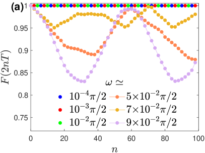
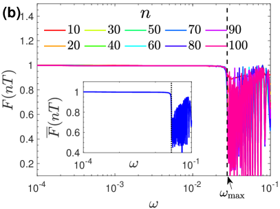
Figure 1: (a) Stroboscopic dynamics of the revival fidelity $F(2nT)$ over a hundred of period cycles $n$ when system of size $L{=}12$ is in the DTC phase, happens for $\omega{\leq}10^{-2}\pi/2$, and non-DTC, happens for $\omega{\geq}0.05\pi/2$. (b) Dynamical behavior of the revival fidelity at stroboscopic times $n{\in}\{10,\cdots,100\}$ as a function of $\omega$ obtained for a chain of size $L{=}30$ and $\varepsilon{=}0.01$. The inset is the average fidelity $\overline{F}(nT)$. The black dashed line determines the onset of the phase transition.

Discrete Time Crystal.– We begin by highlighting some key features of $H_{I}$. First, $H_{I}$ is diagonalized in the computational basis, namely $H_{I}{=}\sum_{\mathbf{z}=1}^{2^{L}}E_{\mathbf{z}}|\mathbf{z}\rangle\langle\mathbf{z}|$ in which $\{|\mathbf{z}\rangle\}$ represents the $2^{L}$ elements of the computational basis. Any state of the computational basis can be written as $|\mathbf{z}\rangle{=}(\sigma_{1}^{x})^{j_{1}}(\sigma_{2}^{x})^{j_{2}}\cdots(\sigma_{L}^{x})^{j_{L}}|{\uparrow,\uparrow,\cdots,\uparrow}\rangle$ with $\mathbf{z}{=}(j_{1},j_{2},\cdots,j_{L})_{2}$ being the binary representation of the integer $\mathbf{z}$. Second, $[H_{I},\Pi_{j}\sigma_{j}^{x}]{=}0$ which implies that $E_{\mathbf{z}}{=}E_{2^{L}-1-\mathbf{z}}$. Third, for an even number of spins which is considered here, all the eigenvalues $E_{\mathbf{z}}$ are integer numbers that are even (odd) if $L{/2}$ is an even (odd) number. Since $[H_{I},\Pi_{j}\sigma_{j}^{x}]{=}0$, for $\varepsilon{=}0$ which results in $e^{-iH_{P}}{=}\Pi_{j}\sigma_{j}^{x}$, one has a trivial period doubling DTC as $U_{F}^{2}(\Omega{=}\pi/2,\varepsilon{=}0){=}e^{-2iH_{P}}e^{-2i\Omega H_{I}}{=}(-1)^{H_{I}}{=}{\pm}\mathbb{I}$. Consequently, one observes persistent oscillations in typical observables with spontaneously breaking DTTS. For $\varepsilon{\neq}0$, one gets $[H_{I},e^{-iH_{P}}]{\neq}0$. In this case, the reduction of $U_{F}^{2}(\Omega{=}\pi/2,\varepsilon{\neq}0)$ to the identity is not obvious. To study this nontrivial DTC, we focus on the evolution of computational basis over $n$ period cycles and its revival fidelity $F(nT){=}|\langle\mathbf{z}|U_{F}^{n}(\Omega{=}\pi/2,\varepsilon{\neq}0)|\mathbf{z}\rangle|^{2}$ in the system with even number of spins. For a typical computational basis state $|\mathbf{z}\rangle$ with $u_{\mathbf{z}}$ spins down, the free evolution of the system governed by $H_{I}$ imposes a dynamical phase as $e^{-i\Omega H_{I}}|\mathbf{z}\rangle{=}(-i)^{L/2}(-1)^{u_{\mathbf{z}}}|\mathbf{z}\rangle$. Then the first rotating pulse evolves $|\mathbf{z}\rangle$ to a superposition of all the $2^{L}$ elements, each with coefficient $(-i\sin\Phi)^{f}(\cos\Phi)^{L-f}$ wherein $f$ is the number of the flipped spins. After the second period of the evolution, one can show that $\langle\mathbf{z}|U_{F}^{2}(\Omega{=}\pi/2,\varepsilon{\neq}0)|\mathbf{z}\rangle$ is equal with the summation of $2^{L}$ choices of flipping $L$ spins with coefficient $(i)^{L}(-i\sin\Phi)^{2f}(\cos\Phi)^{2(L-f)}$. A straightforward simplification results in $\langle\mathbf{z}|U_{F}^{2}(\Omega{=}\pi/2,\varepsilon{\neq}0)|\mathbf{z}\rangle{=}(-i)^{L}$ and, hence, $F(2T){=}1$, see Supplementary Materials (SM). This calculation shows that regardless of the imperfections in the driving pulse, as long as $\Omega{=}\pi/2$ any initial state returns to itself after time $2T$, therefore, period-doubling oscillations of $F(nT)$ persists indefinitely even in finite size systems.

However, establishing a stable DTC must be independent of fine-tuned Hamiltonian parameters. This obliges us to analyze the effect of a deviation as $\omega{=}|\pi/2{-}\Omega|$. Surprisingly, our comprehensive numerical simulations show that as $\omega$ increases, our system goes through a sharp phase transition from a stable DTC to a region with no spontaneous breaking of DTTS in Eq.(1). Before presenting the main results, some general points related to methodologies need to be clarified. Throughout this Letter, we used the exact diagonalization (ED) computational method for the system of size $L{=}12$ and time-dependent variational principle (TDVP) techniques for finite matrix product state (MPS), using PYTHON package TeNPy Hauschild and Pollmann (2018), for systems of size $L{>}12$. The results are presented for the initial state $|\psi_{0}\rangle{=}|\mathbf{0}\rangle{=}|{\uparrow,\cdots,\uparrow\rangle}$, although, the results are generic and remain valid for other computational basis states too (see SM). In Fig. 1(a), we plot stroboscopic dynamics of the revival fidelity $F(2nT)$ as a function of $n$ for different values of $\omega$ in the system of size $L{=}12$ under a driving pulse with an imperfection of magnitude $\varepsilon{=}0.01$. In the stable DTC phase, happening in the range $\omega{\leq}10^{-2}\pi/2$, one observes $F(2nT){=}1$. For larger values of the deviation, such as $\omega{\geq}0.05\pi/2$, revival fidelity shows nontrivial oscillations, signaling the entrance to a non-DTC region. We characterize this region later. This distinctive behavior with respect to $\omega$ reflects itself in all stroboscopic times as has been depicted in Fig. 1(b). In this panel, we plot the revival fidelity at different stroboscopic times $n{\in}\{2,10,\cdots,100\}$, in a chain of length $L{=}30$ and $\varepsilon{=}0.01$. The inset represents the average fidelity $\overline{F}(nT){=}(1/N)\sum_{n=1}^{N}F(2nT)$ for the considered stroboscopic times. As is obvious from Fig. 1(b), the phase transition between stable DTC and non-DTC region occurs at a specific value of $\omega{=}\omega_{\max}$, dashed line, in all the stroboscopic times. In the following, we first analyze the capability of this phase transition as a resource for quantum sensing. Then, we complete this analysis by extracting the critical features of the quantum phase transition using a well-established mechanism that identifies the type of transition as a second-order one.

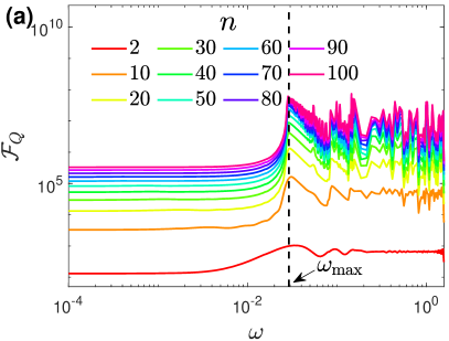
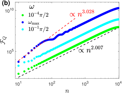
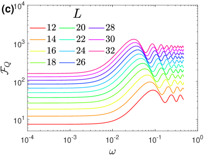
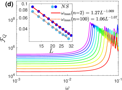
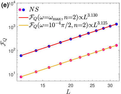
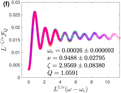
Figure 2: (a) The QFI $\mathcal{F}_{Q}$ versus $\omega$ in stroboscopic times in a system of size $L{=}30$. The onset of the phase transition is determined by $\omega{=}\omega_{\max}$ (dashed line), the point where QFI peaks in different $n$’s. (b) Dynamical growth of the QFI when a system of size $L{=}12$ is deeply in DTC phase (for $\omega{=}10^{-4}\pi/2$), in the non-DTC phase (for $\omega{=}10^{-1}\pi/2$), and at the transition point ($\omega{=}\omega_{\max}$). (c) and (d) QFI versus $\omega$ in systems with various $L$’s after $n{=}2$ and $n{=}100$, respectively. Inset: $\omega_{\max}$ versus $L$ at $n{=}2$ and $n{=}100$. The numerical simulation (NS) are well described by the fitting function $\omega_{\max}{\propto}L^{-1}$. (e) The values of the QFI after $n=2$ in DTC phase (for $\omega{=}10^{-4}\pi/2$) and at transition points ($\omega{=}\omega_{\max}$) versus $L$. The numerical simulation (NS) is well-mapped by a function as $\mathcal{F}_{Q}{\propto}L^{\beta}$ (solid lines) with $\beta{>}3$. (f) The finite-size scaling analysis obtained for the curves in panel (c). The best data collapse is obtained for the reported critical parameters ($\omega_{c},\zeta,\nu$). Here, $Q$ determines the quality of the data collapse with $Q{=}1$ for the optimal data collapse Melchert (2009); Sorge (2015).

DTC sensor.– To investigate the sensing capability of our DTC probe for sensing $\omega$, in Fig. 2(a), we plot QFI $\mathcal{F}_{Q}$ as a function of $\omega$ at different stroboscopic times $n{\in}\{2,10,\cdots,100\}$, in a chain of length $L{=}30$ and $\varepsilon{=}0.01$. Several interesting features can be observed. First, the QFI shows distinct behaviors in each phase. While in the DTC phase, the $\mathcal{F}_{Q}$ becomes a plateau whose value depends on $n$, in the non-DTC region it shows nontrivial and fast oscillations. Second, by approaching the transition point, denoted by $\omega_{\max}$ (dashed line), the QFI indeed shows a clear peak at all stroboscopic times. Note that $\omega_{\max}$ in both Fig. 1(b) and Fig. 2(a) are exactly the same. To understand the dynamical growth of the QFI, in Fig. 2(b), we plot $\mathcal{F}_{Q}$ over thousands of driving cycle $n$ in a systems of size $L{=}12$ and $\varepsilon{=}0.01$ at different $\omega$’s. As the figure shows, when the probe is tuned to work deeply in either DTC phase (for $\omega{=}10^{-4}\pi/2$) or the non-DTC region (for $\omega{=}10^{-1}\pi/2$), one obtains $\mathcal{F}_{Q}{\propto}n^{2}$. However, in the transition point, $\omega{=}\omega_{\max}$ the QFI in the early times $n{\in}[1,\cdots,80]$ dramatically increases as $\mathcal{F}_{Q}{\propto}n^{3}$, and then follows $\mathcal{F}_{Q}{\propto}n^{2}$ in the larger times. To identify the effect of size on quality of sensing, we analyze the QFI at various sizes $L{=}12,\cdots,32$ and also different cycles $n$. In Figs. 2(c) and (d), we plot the obtained $\mathcal{F}_{Q}$ as a function of $\omega$ after $n{=}2$ and $n{=}100$ cycling periods, respectively, for various $L$ and fixed $\varepsilon{=}0.01$. The finite-size effect is obvious in both DTC phase and transition point, namely, the points where QFI peaks. By enlarging the chain, the peaks of the QFI smoothly skew towards smaller values of $\omega$ as can be seen in the inset of Fig. 2(d). The obtained $\omega_{\max}$ at different $n$’s are well-mapped with function $\omega_{\max}{\propto}L^{-1}$, indicating that in the thermodynamic limit $L{\rightarrow}\infty$ the transition happens at infinitesimal deviation $\omega$. In the non-DTC region, the oscillatory behavior of the QFI, in particular in larger times ($n{=}100$) prevents us from investigating the scaling behaviors in this phase. In Fig. 2(e), we present the QFI at $n{=}2$ as a function of $L$ at $\omega{=}10^{-4}\pi/2$, namely deep inside the DTC phase, and also at the corresponding transition points $\omega{=}\omega_{\max}$. The numerical results can be properly mapped with a fitting function as $\mathcal{F}_{Q}{\propto}L^{\beta}$ with $\beta{=}3.125$ and $\beta{=}3.13$ in the DTC phase and at the transition point, respectively. Based on these, one can suggest the following ansatz for the QFI

$$\mathcal{F}_{Q}\propto n^{\alpha}L^{\beta},$$ (4)

where throughout the DTC phase one has $\alpha{\simeq}2$ and $\beta{\simeq}3$. We highlight this as the main result of this Letter showing that our DTC probe achieves quantum-enhanced sensitivity. It is worth emphasizing that in classical probes one at best achieves $\beta{=}1$. Exploiting quantum features may enhance the precision to $\beta{=}2$, conventionally known as the Heisenberg limit. The ultimate obtainable precision in $k$-body interacting system, however, is given by $\beta{=}2k$, which becomes $\beta{=}4$ in our case Boixo et al. (2007). Thus, while our DTC probe beats the conventional Heisenberg limit, it remains below the ultimate precision bound.

To characterize the observed phase transition, we assume a continuous second-order ansatz for the QFI as $\mathcal{F}_{Q}{=}L^{\zeta/\nu}\mathcal{G}(L^{1/\nu}(\omega{-}\omega_{c}))$ where $\zeta$ and $\nu$ are critical exponents, $\omega_{c}$ is the critical point and $\mathcal{G}$ is an arbitrary function. If this ansatz is correct, one expects to obtain data collapse of various size systems when $L^{-\zeta/\nu}\mathcal{F}_{Q}$ is plotted versus $L^{1/\nu}(\omega{-}\omega_{c})$. Indeed, as shown in Fig. 2(f), tuning the parameters to $(\omega_{c},\zeta,\nu){\simeq}(0.00026,2.9569,0.9488)$, optimized using Python package PYFSSA Melchert (2009); Sorge (2015), results in an almost perfect data collapse for curves in Fig. 2(c). This indicates that the DTC phase transition is indeed of the second-order type.

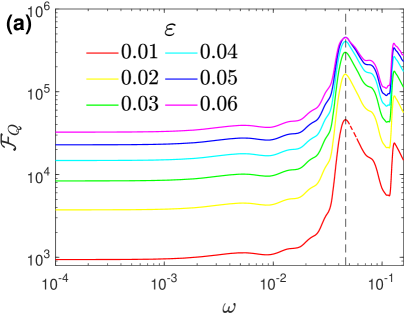
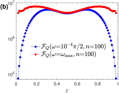
Figure 3: (a) The QFI versus $\omega$ in a chain of size $L{=}20$ after $n{=}10$ period cycles for different $\varepsilon$. The dashed line determines the onset of the phase transition. (b) The QFI versus $\varepsilon$ for two values of $\omega$, obtained after $n{=}100$ cycling periods in a system of size $L{=}12$.

Imperfection effect.– Previously we analytically proved that our DTC is robust against uniform imperfection $\varepsilon$ in the driving pulse when $\omega{=}0$ (see SM). In the case of nonzero $\omega$, the situation becomes even more interesting. In Fig. 3(a), we plot the QFI versus $\omega$ after $n{=}10$ for a chain of size $L{=}20$ under driving pulse with various imperfections $\varepsilon$. While the qualitative behavior of the probe in the DTC phase is not affected by imperfection, increasing $\varepsilon$ may enhance the QFI. To assess the performance in a wider range of the imperfection, in Fig. 3(b) we report $\mathcal{F}_{Q}$ as a function of $\varepsilon$ for $\omega{=}10^{-4}\pi/2$, and $\omega{=}\omega_{\max}$. The results are obtained after $n{=}100$ in a system of size $L{=}12$. This can be understood as imperfect rotating pulses through involving a larger sector of the Hilbert space in the dynamics of the system imprints more information about $\omega$ into the quantum state. The enhancement in the DTC phase, where the system is supposed to be strongly localized, has remarkably stronger effect than at the transition point that already has features of both thermalization and localization. This interesting result is in sharp contrast with the usual sensors where the imperfections deteriorate the sensing power.

Melting transition of the DTC.– Having elucidated the sharp second-order phase transition controlled by $\omega$, we now explore the melting of the DTC by increasing the imperfection $\varepsilon$. In Fig. 4(a), we plot the revival fidelity $F(nT)$ after $n{=}100$ period cycles as a function of $\omega$ and $\varepsilon$, obtained for system of size $L{=}12$. Indeed the phase diagram is fully described by both $\omega$ and $\varepsilon$. To diagnose the transition driven by the imperfection $\varepsilon$, we use averaged entanglement entropy $\langle S_{EE}\rangle$ and averaged diagonal entropy $\langle S_{DE}\rangle$ obtained for all Floquet states of $U_{F}(\Omega,\varepsilon){=}\sum_{k=1}^{2^{L}}e^{-i\phi_{k}}|\phi_{k}\rangle\langle\phi_{k}|$. For a given Floquet state $|\phi_{k}\rangle$, the reduced density matrix $\rho_{L/2}^{(k)}=\mathrm{Tr}_{L/2}|\phi_{k}\rangle\langle\phi_{k}|$ can be obtained by tracing out $L/2$ spins in the right side of the chain. Therefore, the entanglement entropy between the half-systems is $S_{EE}^{(k)}{=}{-}\mathrm{Tr}[\rho_{L/2}^{(k)}\ln(\rho_{L/2}^{(k)})]$ with an average as $\langle S_{EE}\rangle{=}\sum_{k=1}^{2^{L}}S_{EE}^{(k)}/2^{L}$. Replacing $\rho_{L/2}^{(k)}$ by decohered density matrix $\varrho_{L/2}^{(k)}$ which only contain the diagonal elements of $\rho_{L/2}^{(k)}$, results in diagonal entropy as $S_{DE}^{(k)}{=}{-}\mathrm{Tr}[\varrho_{L/2}^{(k)}\ln(\varrho_{L/2}^{(k)})]$ and its average $\langle S_{DE}\rangle{=}\sum_{k=1}^{2^{L}}S_{DE}^{(k)}/2^{L}$. This quantity has recently been proposed for emulating the thermodynamic behavior in many-body localization contexts Yousefjani and Bayat (2023); Yousefjani et al. (2023b). In the DTC phase, each Floquet state is a maximally entangled Greenberger-Horne-Zeilinger (GHZ) of two computational basis states. For instance, for negligible values of the $\varepsilon$, one approximately has $|\phi_{1}\rangle{\cong}\frac{1}{\sqrt{2}}(|\mathbf{0}\rangle+|{\mathbf{2^{L}-1}}\rangle)$ and $|\phi_{2^{L}}\rangle{\cong}\frac{1}{\sqrt{2}}(|\mathbf{0}\rangle-|\mathbf{2^{L}-1}\rangle)$ with the corresponding eigenvalues as $\phi_{1}{\cong}E_{\mathbf{1}}$ and $\phi_{2^{L}}{\cong}E_{\mathbf{1}}\pm\pi$. This so-called $\pi$-pairs of the Floquet states results in $S_{EE}^{(k)}{=}S_{DE}^{(k)}{=}\ln 2$ in deep DTC phase. By increasing $\varepsilon$ both entanglement and diagonal entropy grow and peak at $\varepsilon{=}0.5$, see Fig. 4(b) and also SM. To extract the critical properties of a transition, one can establish finite-size scaling analysis to predict the behavior of the system when its size is changing. In the inset of Fig. 4(b), we depict the best collapse of the corresponding curves obtained for reported $(\varepsilon_{c},\nu,\zeta)$. By increasing the system size $\omega_{\max}$ decreases and thus the extension of the DTC phase becomes smaller. Therefore, for finite-size scaling analysis we select the lengths such that for the given $\omega$ they are all within the DTC phase when $\varepsilon{\simeq}0$. Note that the obtained $\varepsilon_{c}$ from finite-size scaling of both $\langle S_{EE}\rangle$ and $\langle S_{DE}\rangle$, shown as markers on panel (a), are very close and determine the phase boundary between the DTC and the non-DTC phase.

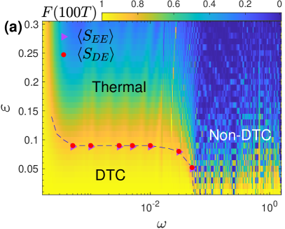
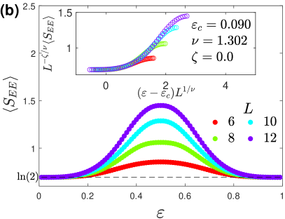
Figure 4: (a) Phase diagram of the DTC as function of $\omega$ and $\varepsilon$. The background is $F(nT)$ after $n{=}100$ in a system of size $L{=}12$. The markers determine the phase boundary between DTC and the thermal phase, obtained through finite-size scaling analysis of averaged entanglement entropy $\langle S_{EE}\rangle$ and averaged diagonal entropy $\langle S_{DE}\rangle$. (b) $\langle S_{EE}\rangle$ versus $\varepsilon$ for systems of different sizes at $\omega{=}5{\times}10^{-4}$. Inset is the finite-size scaling analysis, showing the best data collapse obtained for reported critical parameters $(\varepsilon_{c},\nu,\zeta)$.

Non-DTC region.– By increasing $\omega$, one observes non trivial oscillations in the behvior of fidelity $F(2nT)$, see Fig. 1(a), which signals the lost of the DTC order. As the system size increases the period of these oscillations increases, hinting that the system thermalizes in the thermodynamic limit $L{\rightarrow}\infty$. As shown in the SM, the entanglement entropy $\langle S_{EE}\rangle$ and the diagonal entropy $\langle S_{DE}\rangle$ asymptotically approach their corresponding Page entropy Page (1993); Torres-Herrera and Santos (2017); Torres-Herrera et al. (2016), expected for ergodic thermal phases, as the system size increases. This provides further evidence that the non-DTC phase becomes an ergodic thermal phase in the thermodynamic limit.

Conclusion.– Having established a DTC with indefinite persistent oscillations and strong robustness to the imperfections in the driving pulse, we show that this DTC is extremely precise in measuring coupling strength. It provide quantum-enhanced sensing over a region that extends over the DTC phase to the transition point. Through establishing finite-size scaling analysis, we characterize the nature of the phase transition as the second-order and determine relevant critical exponents. The obtained quantum-enhanced sensitivity is general and independent of the initial state. Regarding the imperfection in the rotating pulse, we show that increasing imperfection, before melting the DTC, enhances the precision of estimation in both DTC phase and transition point.

Acknowledgement.– We thank Fernando Iemini for insightful comments. A.B. acknowledges support from the National Natural Science Foundation of China (Grants No. 12050410253, No. 92065115, and No. 12274059), and the Ministry of Science and Technology of China (Grant No. QNJ2021167001L). R. Y. acknowledges support from the National Science Foundation of China for the International Young Scientists Fund (Grant No. 12250410242). This research was funded by the National Science Centre, Poland, Projects No. 2021/42/A/ST2/ 00017 (K.S.).

Supplementary Materials

I Robustness of the DTC against nonuniform imperfections

In the main text, we analytically show that in the case of $\Omega{=}\pi/2$, our DTC is robust against uniform imperfection defined as $\Phi=(1-\varepsilon)\frac{\pi}{2}$. In general, this imperfection can be nonuniform, namely it varies from site to site. In this scenario, the total imperfection $\Phi$ in $H_{P}$ (Eq. (2) of the main text) can be replaced by $\Phi_{j}=(1-\varepsilon_{j})\frac{\pi}{2}$ with $\varepsilon_{j}$ as a random number which is selected from a uniform distribution as $[-\varepsilon,\varepsilon]$ with $\varepsilon{\neq}0$. To see the effect of this nonuniform imperfection on the DTC in the case $\Omega{=}\pi/2$, we focus on the revival fidelity of a typical computational basis $|\mathbf{z}\rangle$. Assume that $u_{\mathbf{z}}$ denotes the number of spins down in $|\mathbf{z}\rangle$, therefore the free evolution of the system governed by $H_{I}$ imposes a dynamical phase as $e^{-i\Omega H_{I}}|\mathbf{z}\rangle{=}(-i)^{L/2}(-1)^{u_{\mathbf{z}}}|\mathbf{z}\rangle$. Then the first driving pulse evolves $|\mathbf{z}\rangle$ to a combination of $2^{L}$ computational basis, each with coefficient $\Pi_{j{\in}A}\Pi_{j^{{}^{\prime}}\in\tilde{A}}(-i\cos(\varepsilon_{j})\sin(\varepsilon_{j^{{}^{\prime}}}))$ wherein $A$ ($\tilde{A}$) are the collection of the unflipped (flipped) spins and $A{\cup}\tilde{A}{=}\{1,\cdots,L\}$. Followed by the second period of evolution, one can show that $\langle\mathbf{z}|U_{F}^{2}(\Omega{=}\pi/2,\varepsilon{\neq}0)|\mathbf{z}\rangle$ is equal with the summation of $2^{L}$ choices of flipping $L$ spins with coefficient $(i)^{L}\Pi_{j{\in}A}\cos^{2}(\varepsilon_{j})\Pi_{j^{{}^{\prime}}\in\tilde{A}}\sin^{2}(\varepsilon_{j^{{}^{\prime}}})$. A straightforward simplification results in $\langle\mathbf{z}|U_{F}^{2}(\Omega{=}\pi/2,\varepsilon{\neq}0)|\mathbf{z}\rangle{=}(-i)^{L}$ and, hence, $F(2T){=}1$. This calculation shows that regardless of the imperfections in the driving pulse, as long as $\Omega{=}\pi/2$ any initial state returns to itself after time $2T$, therefore, period-doubling oscillations of the revival fidelity resist indefinitely even in finite size systems. In the following, through an illustrative example, we provide more details on revival fidelity in a system of size $L{=}4$ prepared initially in $|\mathbf{5}\rangle{=}|{\uparrow\downarrow\uparrow\downarrow}\rangle$. In fact we aim to calculate $F(2T)=|\langle\mathbf{5}|U^{2}(\Omega{=}\pi/2,\varepsilon{\neq}0)|\mathbf{5}\rangle|^{2}$. Note that here $c_{j}$ and $s_{j}$ are abbreviations for $\cos(\Phi_{j})$ and $\sin(\Phi_{j})$, respectively.

$$e^{-i\Omega H_{I}}|\mathbf{5}\rangle= (-i)^{L/2}(-1)^{2}|\mathbf{5}\rangle$$ (S1)

$$e^{-iH_{p}}e^{-i\Omega H_{I}}|\mathbf{5}\rangle= (-i)^{L/2}\Big{\{}c_{1}c_{2}c_{3}c_{4}|\mathbf{5}\rangle+(-i)c_{1}c_{2}c_{3}s_{4}|\mathbf{4}\rangle+(-i)c_{1}c_{2}s_{3}c_{4}|\mathbf{7}\rangle+(-i)^{2}c_{1}c_{2}s_{3}s_{4}|\mathbf{6}\rangle$$ (S2)

$$+ (-i)c_{1}s_{2}c_{3}c_{4}|\mathbf{1}\rangle+(-i)^{2}c_{1}s_{2}c_{3}s_{4}|\mathbf{0}\rangle+(-i)^{2}c_{1}s_{2}s_{3}c_{4}|\mathbf{3}\rangle+(-i)^{3}c_{1}s_{2}s_{3}s_{4}|\mathbf{2}\rangle$$ (S3)

$$+ (-i)s_{1}c_{2}c_{3}c_{4}|\mathbf{13}\rangle+(-i)^{2}s_{1}c_{2}c_{3}s_{4}|\mathbf{12}\rangle+(-i)^{2}s_{1}c_{2}s_{3}c_{4}|\mathbf{15}\rangle+(-i)^{3}s_{1}c_{2}s_{3}s_{4}|\mathbf{14}\rangle$$ (S4)

$$+ (-i)^{2}s_{1}s_{2}c_{3}c_{4}|\mathbf{9}\rangle+(-i)^{3}s_{1}s_{2}c_{3}s_{4}|\mathbf{8}\rangle+(-i)^{3}s_{1}s_{2}s_{3}c_{4}|\mathbf{11}\rangle+(-i)^{4}s_{1}s_{2}s_{3}s_{4}|\mathbf{10}\rangle\Big{\}}$$ (S5)

$$e^{-i\Omega H_{I}}e^{-iH_{p}}e^{-i\Omega H_{I}}|\mathbf{5}\rangle= (-i)^{L}\Big{\{}(-1)^{2}c_{1}c_{2}c_{3}c_{4}|\mathbf{5}\rangle+(-1)^{1}(-i)c_{1}c_{2}c_{3}s_{4}|\mathbf{4}\rangle+(-1)^{3}(-i)c_{1}c_{2}s_{3}c_{4}|\mathbf{7}\rangle+(-1)^{2}(-i)^{2}c_{1}c_{2}s_{3}s_{4}|\mathbf{6}\rangle$$ (S7)

$$+ (-1)^{1}(-i)c_{1}s_{2}c_{3}c_{4}|\mathbf{1}\rangle+(-1)^{0}(-i)^{2}c_{1}s_{2}c_{3}s_{4}|\mathbf{0}\rangle+(-1)^{2}(-i)^{2}c_{1}s_{2}s_{3}c_{4}|\mathbf{3}\rangle+(-1)^{1}(-i)^{3}c_{1}s_{2}s_{3}s_{4}|\mathbf{2}\rangle$$ (S8)

$$+ (-1)^{3}(-i)s_{1}c_{2}c_{3}c_{4}|\mathbf{13}\rangle+(-1)^{2}(-i)^{2}s_{1}c_{2}c_{3}s_{4}|\mathbf{12}\rangle+(-1)^{4}(-i)^{2}s_{1}c_{2}s_{3}c_{4}|\mathbf{15}\rangle+(-1)^{3}(-i)^{3}s_{1}c_{2}s_{3}s_{4}|\mathbf{14}\rangle$$ (S9)

$$+ (-1)^{2}(-i)^{2}s_{1}s_{2}c_{3}c_{4}|\mathbf{9}\rangle+(-1)^{1}(-i)^{3}s_{1}s_{2}c_{3}s_{4}|\mathbf{8}\rangle+(-1)^{3}(-i)^{3}s_{1}s_{2}s_{3}c_{4}|\mathbf{11}\rangle+(-1)^{2}(-i)^{4}s_{1}s_{2}s_{3}s_{4}|\mathbf{10}\rangle\Big{\}}$$ (S10)

$$e^{-iH_{p}}e^{-i\Omega H_{I}}e^{-iH_{p}}e^{-i\Omega H_{I}}|\mathbf{5}\rangle= (-i)^{L}\Big{\{}(c_{1}c_{2}c_{3}c_{4})^{2}+(c_{1}c_{2}c_{3}s_{4})^{2}+(c_{1}c_{2}s_{3}c_{4})^{2}+(c_{1}c_{2}s_{3}s_{4})^{2}+(c_{1}s_{2}c_{3}c_{4})^{2}+(c_{1}s_{2}c_{3}s_{4})^{2}$$ (S12)

$$+ (c_{1}s_{2}s_{3}c_{4})^{2}+(c_{1}s_{2}s_{3}s_{4})^{2}+(s_{1}c_{2}c_{3}c_{4})^{2}+(s_{1}c_{2}c_{3}s_{4})^{2}+(s_{1}c_{2}s_{3}c_{4})^{2}+(s_{1}c_{2}s_{3}s_{4})^{2}$$ (S13)

$$+ (s_{1}s_{2}c_{3}c_{4})^{2}+(s_{1}s_{2}c_{3}s_{4})^{2}+(s_{1}s_{2}s_{3}c_{4})^{2}+(s_{1}s_{2}s_{3}s_{4})^{2}\Big{\}}|\mathbf{5}\rangle+\cdots$$ (S14)

$$e^{-iH_{p}}e^{-i\Omega H_{I}}e^{-iH_{p}}e^{-i\Omega H_{I}}|\mathbf{5}\rangle= (-i)^{L}|\mathbf{5}\rangle+\cdots$$ (S16)

Therefore, one has $F(2T)=|\langle\mathbf{5}|U^{2}(\Omega{=}\pi/2,\varepsilon{\neq}0)|\mathbf{5}\rangle|^{2}=1$.

II Role of initial state and imperfection effect

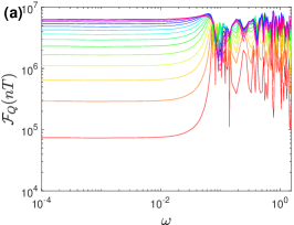
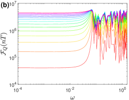
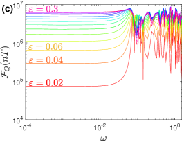
Figure S1: (a)-(c) The QFI after $n{=}100$ period cycles as a function of deviation $\omega$ obtained for different values of $\varepsilon{\in}\{0.02,0.04,\cdots,0.3\}$ in a chain of size $L{=}12$ that is initialized in $|\psi_{0}\rangle{=}|\mathbf{0}\rangle{=}|{\uparrow,\uparrow,\cdots,\uparrow}\rangle$, a random state, and Néel state $|\psi_{0}\rangle{=}|\mathbf{1365}\rangle{=}|{\uparrow,\downarrow,\cdots,\uparrow,\downarrow}\rangle$, respectively.

In the main text, we present results only for the initial state $|\psi_{0}\rangle{=}|\mathbf{0}\rangle{=}|{\uparrow,\cdots,\uparrow}\rangle$. In this section, we provide results for other computational states to show the generality of the observed behavior concerning $\omega$ and $\varepsilon$. In Fig. S1, we depict the QFI $\mathcal{F}_{Q}(nT)$ as a function of $\omega$ after $n{=}100$ period cycles in a system of size $L{=}12$, initialized in (a) $|\psi_{0}\rangle{=}|{\uparrow,\cdots,\uparrow}\rangle$, (b) a random state, and (c) the Néel state $|\psi_{0}\rangle{=}|{\uparrow,\downarrow\cdots,\uparrow,\downarrow}\rangle$. Curves with different colors correspond to different values of imperfections $\varepsilon$. In terms of $\omega$, one can see that the distinctive behavior of our system in both DTC and non-DTC phases reflects itself in all the considered initial states. Regarding the imperfection effect, by increasing $\varepsilon$, more information about $\omega$ can be printed in the evolved state, resulting in higher values of the QFI. As is clear from Fig. S1, this behavior is qualitatively independent of the initial states.

III Melting transition of the DTC

In the main text, we show how increasing imperfection in the rotating pulse $\varepsilon$ can onset a phase transition between stable DTC and non-DTC phase. The transition driven by $\varepsilon$ is diagnosed by averaged entanglement entropy $\langle S_{EE}\rangle$ and averaged diagonal entropy $\langle S_{DE}\rangle$ obtained for all Floquet states of $U_{F}(\Omega,\varepsilon){=}\sum_{k=1}^{2^{L}}e^{-i\phi_{k}}|\phi_{k}\rangle\langle\phi_{k}|$. In the DTC phase, each Floquet state $|\phi_{k}\rangle$ is a maximally entangled GHZ state of a pair of computational basis states. For instance for small values of $\varepsilon$ one approximately has $|\phi_{1}\rangle{\cong}\frac{1}{\sqrt{2}}(|\mathbf{0}\rangle+|\mathbf{2^{L}-1}\rangle)$ and $|\phi_{2^{L}}\rangle{\cong}\frac{1}{\sqrt{2}}(|\mathbf{0}\rangle-|\mathbf{2^{L}-1}\rangle)$ with the corresponding eigenvalues as $\phi_{1}{\cong}E_{\mathbf{0}}$ and $\phi_{2^{L}}{\cong}E_{\mathbf{0}}\pm\pi$. Note that $\{E_{\mathbf{z}}\}$ are the eigenvalues of $H_{I}$ with $E_{\mathbf{z}}{=}E_{2^{L}-1-\mathbf{z}}$. Clearly, deep inside the DTC regime, the entanglement entropy is $S_{EE}^{(k)}{\cong}\ln 2$ for all $k$’s. This can be seen in Fig. S2 (a)-(c) which depict the averaged entanglement entropy $\langle S_{EE}\rangle$ for systems of various sizes and $\omega\in\{1,3,5\}\times 10^{-2}$. In this regime, by enlarging $\varepsilon$ the averaged entanglement entropy gets distance from $\ln 2$ and peaks at its size- and $\omega$-dependent location, happening for $\varepsilon{=}0.5$. The behavior of the entanglement entropy concerning $L$ hints that the melting transition is of second-order type. This means that one can extract the critical properties for the transition by implementing finite-size scaling analysis. However, as $\omega_{\max}{\propto}L^{-1}$, by increasing the system size the range of $\omega$’s that the DTC phase is stable for them, namely $\omega{<}\omega_{\max}$, shrinks. Therefore, the results for finite-size scaling analysis obtained using probes that for any given $\omega{<}\omega_{\max}$ these systems are within the DTC phase when $\varepsilon{\simeq}0$. Here, the numerical restriction in the ED method limits us to the system up to $L{=}12$. Presuming that the averaged entanglement entropy follows an ansatz as $\langle S_{EE}\rangle=L^{\zeta/\nu}\mathcal{D}(L^{1/\nu}(\varepsilon-\varepsilon_{c}))$, then plotting $L^{-\zeta/\nu}\langle S_{EE}\rangle$ as a function of $L^{1/\nu}(\varepsilon-\varepsilon_{c})$ collapses the curves of different sizes. Here, $\zeta$ and $\nu$ are the critical exponents, $\varepsilon_{c}$ is the critical point, and $\mathcal{D}$ is an arbitrary function. The best data collapse can be obtained for the optimal critical parameters $(\varepsilon_{c},\zeta,\nu)$. In the insets of Fig. S2(a)-(c), we present the best data collapse of the corresponding curves obtained for the reported critical parameters. For the sake of completeness, we repeat the analysis above for the averaged diagonal entropy. The diagonal entropy contains partial information about the system by setting the off-diagonal terms of the half-system reduced density matrix to zero. In Fig. S2(d)-(f), we present the obtained $\langle S_{DE}\rangle$ for various sizes and $\omega$’s. Indeed, the behavior of the averaged diagonal entropy is qualitatively close to the averaged entanglement entropy in both DTC and non-DTC phases. In particular, for small values of $\varepsilon$, one has $S_{EE}^{(k)}=S_{DE}^{(k)}=\ln 2$. In the insets of Fig. S2(d)-(f), we present the results of the finite-size scaling analysis that we established for this quantity. Surprisingly the obtained $\varepsilon_{c}$ for both $\langle S_{EE}\rangle$ and $\langle S_{DE}\rangle$ are close. Note that in the transition between the DTC and non-DTC phases driven by $\varepsilon$, one may not observe quantum-enhanced sensitivity in the process of sensing $\varepsilon$.

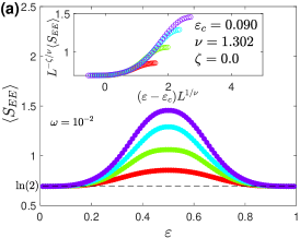
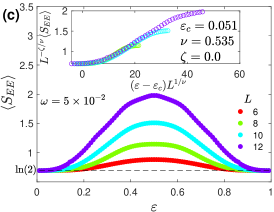
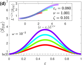
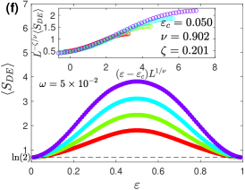
Figure S2: (a)-(c) the averaged entanglement entropy $\langle S_{EE}\rangle$ as a function of pulse imperfection $\varepsilon$ obtained for systems of different sizes and different $\omega$’s. (d)-(f) The averaged diagonal entropy $\langle S_{DE}\rangle$ as a function of $\varepsilon$ in systems with various size and $\omega$’s. The insets of the panels show the results of the finite-size scaling analysis and optimal data collapse of curves with different sizes, which happen for the reported critical properties $(\varepsilon_{c},\nu,\zeta)$.

IV Characterizing the non-DTC region

As has been discussed in the main text, by increasing the divination $\omega$, the perfect and stable revivals of the fidelity in stroboscopic times, namely $F(2nT){=}1$ for $\omega{\leq}\omega_{\max}$, are replaced by nontrivial oscillations for $\omega{>}\omega_{\max}$. This hints one enters a non-DTC region. In this section we aim to characterize the nature of this region. Our results for the revival fidelity $F(2nT)$ as a function of $n$ for systems of different sizes that are tuned to work in the non-DTC region, namely for $\omega{\simeq}0.15$, have been illustrated in Fig. S3(a). By enlarging the system size, the period of these incommensurate fluctuations increases. This implies that, in systems with enough large sizes, these oscillations practically vanish in a reasonable time window, signaling the thermalization of the system. This observation receives more support from our static study based on the entanglement entropy and diagonal entropy. In a thermal system, the Floquet states $\{|\phi_{k}\rangle\}$ are expected to behave as a typical random pure state, therefore their entanglement entropy is predicted to follow the Page entropy $\langle S^{P}_{EE}\rangle{\simeq}(L\ln(2)-1)/2$ for enough large $L$’s. In this case, the average entanglement entropy should already captured its maximum and the variations of $\varepsilon$ may not considerably affect $\langle S^{P}_{EE}\rangle$. Our numerical results in Fig. S3(b) support this prediction for $\omega{=}\frac{\pi}{4}$, namely deep inside the thermal phase. The results for systems of size $L{=}8$ and $L{=}12$ capture the Page entropy $\langle S_{EE}\rangle{\simeq}\langle S^{P}_{EE}\rangle$ (depicted by colored dashed lines) with slight changes in terms of $\varepsilon$. Regarding the diagonal entropy, typical random pure states are expected to follow $\langle S^{P}_{DE}\rangle{\simeq}\ln(0.48\times 2^{L/2})+\ln(2)$. The presented results in Fig. S3(c) confirm this behavior. In this panel $\langle S^{P}_{DE}\rangle$ is represented by colored dashed lines.

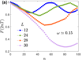
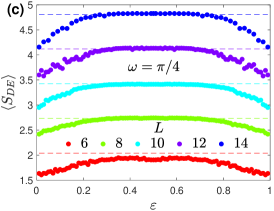
Figure S3: (a) the stroboscopic dynamics of the revival fidelity $F(2nT)$ over $100$ period cycles when systems with different sizes evolve in non-DTC region with $\omega{\simeq}0.15$ and $\varepsilon{=}0.01$. (b) the averaged entanglement entropy $\langle S_{EE}\rangle$ and (c) the averaged diagonal entropy $\langle S_{DE}\rangle$ as a function of pulse imperfection $\varepsilon$ obtained for systems of different sizes and $\omega{=}\pi/4$. Dashed lines in (b) and (c) determine the corresponding $\langle S^{P}_{EE}\rangle$ and $\langle S^{P}_{DE}\rangle$, respectively.

References

- Wilczek (2012) F. Wilczek, Phys. Rev. Lett. 109, 160401 (2012).
- Bruno (2013) P. Bruno, Phys. Rev. Lett. 111, 070402 (2013).
- Watanabe and Oshikawa (2015) H. Watanabe and M. Oshikawa, Phys. Rev. Lett. 114, 251603 (2015).
- Kozin and Kyriienko (2019) V. K. Kozin and O. Kyriienko, Phys. Rev. Lett. 123, 210602 (2019).
- Sacha (2015) K. Sacha, Phys. Rev. A 91, 033617 (2015).
- Khemani et al. (2016) V. Khemani, A. Lazarides, R. Moessner, and S. L. Sondhi, Phys. Rev. Lett. 116, 250401 (2016).
- Else et al. (2016) D. V. Else, B. Bauer, and C. Nayak, Phys. Rev. Lett. 117, 090402 (2016).
- Yao et al. (2017) N. Y. Yao, A. C. Potter, I.-D. Potirniche, and A. Vishwanath, Phys. Rev. Lett. 118, 030401 (2017).
- Russomanno et al. (2017) A. Russomanno, F. Iemini, M. Dalmonte, and R. Fazio, Phys. Rev. B 95, 214307 (2017).
- Ho et al. (2017) W. W. Ho, S. Choi, M. D. Lukin, and D. A. Abanin, Phys. Rev. Lett. 119, 010602 (2017).
- Huang et al. (2018) B. Huang, Y.-H. Wu, and W. V. Liu, Phys. Rev. Lett. 120, 110603 (2018).
- Matus and Sacha (2019) P. Matus and K. Sacha, Phys. Rev. A 99, 033626 (2019).
- Kshetrimayum et al. (2020) A. Kshetrimayum, J. Eisert, and D. Kennes, Phys. Rev. B 102, 195116 (2020).
- Estarellas et al. (2020) M. P. Estarellas, T. Osada, V. M. Bastidas, B. Renoust, K. Sanaka, W. J. Munro, and K. Nemoto, Sci. Adv. 6, eaay8892 (2020).
- Maskara et al. (2021) N. Maskara, A. A. Michailidis, W. W. Ho, D. Bluvstein, S. Choi, M. D. Lukin, and M. Serbyn, Phys. Rev. Lett. 127, 090602 (2021).
- Wang et al. (2021) J. Wang, P. Hannaford, and B. J. Dalton, New J. Phys. 23, 063012 (2021).
- Pizzi et al. (2021) A. Pizzi, J. Knolle, and A. Nunnenkamp, Nat. Commun. 12, 2341 (2021).
- Collura et al. (2022) M. Collura, A. De Luca, D. Rossini, and A. Lerose, Phys. Rev. X 12, 031037 (2022).
- Huang et al. (2022) B. Huang, T.-H. Leung, D. M. Stamper-Kurn, and W. V. Liu, Phys. Rev. Lett. 129, 133001 (2022).
- Bull et al. (2022) K. Bull, A. Hallam, Z. Papić, and I. Martin, Phys. Rev. Lett. 129, 140602 (2022).
- Deng and Yang (2023) W. Deng and Z.-C. Yang, Phys. Rev. B 108, 205129 (2023).
- Liu et al. (2023) S. Liu, S.-X. Zhang, C.-Y. Hsieh, S. Zhang, and H. Yao, Phys. Rev. Lett. 130, 120403 (2023).
- Huang (2023) B. Huang, Phys. Rev. B 108, 104309 (2023).
- Giergiel et al. (2023) K. Giergiel, J. Wang, B. J. Dalton, P. Hannaford, and K. Sacha, Phys. Rev. B 108, L180201 (2023).
- Zhang et al. (2017) J. Zhang, P. W. Hess, A. Kyprianidis, P. Becker, A. Lee, J. Smith, G. Pagano, I.-D. Potirniche, A. C. Potter, A. Vishwanath, et al., Nature 543, 217 (2017).
- Choi et al. (2017) S. Choi, J. Choi, R. Landig, G. Kucsko, H. Zhou, J. Isoya, F. Jelezko, S. Onoda, H. Sumiya, V. Khemani, et al., Nature 543, 221 (2017).
- Pal et al. (2018) S. Pal, N. Nishad, T. Mahesh, and G. Sreejith, Phys. Rev. Lett. 120, 180602 (2018).
- Rovny et al. (2018) J. Rovny, R. L. Blum, and S. E. Barrett, Phys. Rev. Lett. 120, 180603 (2018).
- Smits et al. (2018) J. Smits, L. Liao, H. Stoof, and P. van der Straten, Physi. Rev. Lett. 121, 185301 (2018).
- Randall et al. (2021) J. Randall, C. Bradley, F. Van Der Gronden, A. Galicia, M. Abobeih, M. Markham, D. Twitchen, F. Machado, N. Yao, and T. Taminiau, Science 374, 1474 (2021).
- Keßler et al. (2021) H. Keßler, P. Kongkhambut, C. Georges, L. Mathey, J. G. Cosme, and A. Hemmerich, Phys. Rev. Lett. 127, 043602 (2021).
- Xu et al. (2021) H. Xu, J. Zhang, J. Han, Z. Li, G. Xue, W. Liu, Y. Jin, and H. Yu (2021), eprint arXiv:2108.00942.
- Kyprianidis et al. (2021) A. Kyprianidis, F. Machado, W. Morong, P. Becker, K. S. Collins, D. V. Else, L. Feng, P. W. Hess, C. Nayak, G. Pagano, et al., Science 372, 1192 (2021).
- Taheri et al. (2022) H. Taheri, A. B. Matsko, L. Maleki, and K. Sacha, Nat. Commun. 13, 848 (2022).
- Mi et al. (2022) X. Mi, M. Ippoliti, C. Quintana, A. Greene, Z. Chen, J. Gross, F. Arute, K. Arya, J. Atalaya, R. Babbush, et al., Nature 601, 531 (2022).
- Frey and Rachel (2022) P. Frey and S. Rachel, Sci. Adv. 8, eabm7652 (2022).
- Bao et al. (2024) Z. Bao, S. Xu, Z. Song, K. Wang, L. Xiang, Z. Zhu, J. Chen, F. Jin, X. Zhu, Y. Gao, et al., arXiv:2401.08284 (2024).
- Shinjo et al. (2024) K. Shinjo, K. Seki, T. Shirakawa, R.-Y. Sun, and S. Yunoki, arXiv:2403.16718 (2024).
- Liu et al. (2024a) B. Liu, L.-H. Zhang, Z.-K. Liu, J. Zhang, Z.-Y. Zhang, S.-Y. Shao, Q. Li, H.-C. Chen, Y. Ma, T.-Y. Han, et al., arXiv:2402.13657 (2024a).
- Liu et al. (2024b) B. Liu, L.-H. Zhang, Y. Ma, T.-Y. Han, Q.-F. Wang, J. Zhang, Z.-Y. Zhang, S.-Y. Shao, Q. Li, H.-C. Chen, et al., arXiv:2404.12180 (2024b).
- Sacha and Zakrzewski (2017) K. Sacha and J. Zakrzewski, Rep. Prog. Phys. 81, 016401 (2017).
- Else et al. (2020) D. V. Else, C. Monroe, C. Nayak, and N. Y. Yao, Annu. Rev. Condens. Matter Phys. 11, 467 (2020).
- Khemani et al. (2019) V. Khemani, R. Moessner, and S. Sondhi, arXiv:1910.10745 (2019).
- Sacha (2020) K. Sacha, Time Crystals (Springer International Publishing, Switzerland, Cham, 2020), ISBN 978-3-030-52523-1.
- Hannaford and Sacha (2022) P. Hannaford and K. Sacha, AAPPS Bull. 32, 12 (2022).
- Zaletel et al. (2023) M. P. Zaletel, M. Lukin, C. Monroe, C. Nayak, F. Wilczek, and N. Y. Yao, Rev. Mod. Phys. 95, 031001 (2023).
- Bomantara and Gong (2018) R. W. Bomantara and J. Gong, Phys. Rev. Lett. 120, 230405 (2018).
- Carollo et al. (2020) F. Carollo, K. Brandner, and I. Lesanovsky, Phys. Rev. Lett. 125, 240602 (2020).
- Lyu et al. (2020) C. Lyu, S. Choudhury, C. Lv, Y. Yan, and Q. Zhou, Phys. Rev. Res. 2, 033070 (2020).
- Iemini et al. (2023) F. Iemini, R. Fazio, and A. Sanpera, arXiv:2306.03927 (2023).
- Montenegro et al. (2023) V. Montenegro, M. G. Genoni, A. Bayat, and M. G. Paris, Commun. Phys. 6, 304 (2023).
- Raghunandan et al. (2018) M. Raghunandan, J. Wrachtrup, and H. Weimer, Phys. Rev. Lett. 120, 150501 (2018).
- Heugel et al. (2019) T. L. Heugel, M. Biondi, O. Zilberberg, and R. Chitra, Phys. Rev. Lett. 123, 173601 (2019).
- Yang and Jacob (2019) L.-P. Yang and Z. Jacob, J. Appl. Phys. 126, 174502 (2019).
- Zanardi and Paunković (2006) P. Zanardi and N. Paunković, Phys. Rev. E 74, 031123 (2006).
- Zanardi et al. (2007) P. Zanardi, H. Quan, X. Wang, and C. Sun, Phys. Rev. A 75, 032109 (2007).
- Gu et al. (2008) S.-J. Gu, H.-M. Kwok, W.-Q. Ning, H.-Q. Lin, et al., Phys. Rev. B 77, 245109 (2008).
- Zanardi et al. (2008) P. Zanardi, M. G. Paris, and L. C. Venuti, Phys. Rev. A 78, 042105 (2008).
- Invernizzi et al. (2008) C. Invernizzi, M. Korbman, L. C. Venuti, and M. G. Paris, Phys. Rev. A 78, 042106 (2008).
- Gu (2010) S.-J. Gu, Int. J. Mod. Phys. B 24, 4371 (2010).
- Gammelmark and Mølmer (2011) S. Gammelmark and K. Mølmer, New J. Phys. 13, 053035 (2011).
- Skotiniotis et al. (2015) M. Skotiniotis, P. Sekatski, and W. Dür, New J. Phys. 17, 073032 (2015).
- Rams et al. (2018) M. M. Rams, P. Sierant, O. Dutta, P. Horodecki, and J. Zakrzewski, Phys. Rev. X 8, 021022 (2018).
- Wei (2019) B.-B. Wei, Phys. Rev. A 99, 042117 (2019).
- Chu et al. (2021) Y. Chu, S. Zhang, B. Yu, and J. Cai, Phys. Rev. Lett. 126, 010502 (2021).
- Liu et al. (2021) R. Liu, Y. Chen, M. Jiang, X. Yang, Z. Wu, Y. Li, H. Yuan, X. Peng, and J. Du, npj Quantum Inf. 7, 1 (2021).
- Montenegro et al. (2021) V. Montenegro, U. Mishra, and A. Bayat, Phys. Rev. Lett. 126, 200501 (2021).
- Mirkhalaf et al. (2021) S. S. Mirkhalaf, D. B. Orenes, M. W. Mitchell, and E. Witkowska, Phys. Rev. A 103, 023317 (2021).
- Di Candia et al. (2021) R. Di Candia, F. Minganti, K. Petrovnin, G. Paraoanu, and S. Felicetti, arXiv:2107.04503 (2021).
- Salvia et al. (2023) R. Salvia, M. Mehboudi, and M. Perarnau-Llobet, Phys. Rev. Lett. 130, 240803 (2023).
- Fernández-Lorenzo and Porras (2017) S. Fernández-Lorenzo and D. Porras, Phys. Rev. A 96, 013817 (2017).
- Baumann et al. (2010) K. Baumann, C. Guerlin, F. Brennecke, and T. Esslinger, Nature 464, 1301 (2010).
- Baden et al. (2014) M. P. Baden, K. J. Arnold, A. L. Grimsmo, S. Parkins, and M. D. Barrett, Phys. Rev. Lett. 113, 020408 (2014).
- Klinder et al. (2015) J. Klinder, H. Keßler, M. Wolke, L. Mathey, and A. Hemmerich, Proc. Natl. Acad. Sci. U.S.A. 112, 3290 (2015).
- Rodriguez et al. (2017) S. Rodriguez, W. Casteels, F. Storme, N. C. Zambon, I. Sagnes, L. Le Gratiet, E. Galopin, A. Lemaître, A. Amo, C. Ciuti, et al., Phys. Rev. Lett. 118, 247402 (2017).
- Fitzpatrick et al. (2017) M. Fitzpatrick, N. M. Sundaresan, A. C. Li, J. Koch, and A. A. Houck, Phys. Rev. X 7, 011016 (2017).
- Fink et al. (2017) J. M. Fink, A. Dombi, A. Vukics, A. Wallraff, and P. Domokos, Phys. Rev. X 7, 011012 (2017).
- Ilias et al. (2022) T. Ilias, D. Yang, S. F. Huelga, and M. B. Plenio, PRX Quantum 3, 010354 (2022).
- Ilias et al. (2024) T. Ilias, D. Yang, S. F. Huelga, and M. B. Plenio, npj Quantum Inf. 10, 36 (2024).
- Alipour et al. (2014) S. Alipour, M. Mehboudi, and A. T. Rezakhani, Phys. Rev. Lett. 112, 120405 (2014).
- Budich and Bergholtz (2020) J. C. Budich and E. J. Bergholtz, Phys. Rev. Lett. 125, 180403 (2020).
- Sarkar et al. (2022) S. Sarkar, C. Mukhopadhyay, A. Alase, and A. Bayat, Phys. Rev. Lett. 129, 090503 (2022).
- Koch and Budich (2022) F. Koch and J. C. Budich, Phys. Rev. Res. 4, 013113 (2022).
- Yu et al. (2024) M. Yu, X. Li, Y. Chu, B. Mera, F. N. Ünal, P. Yang, Y. Liu, N. Goldman, and J. Cai, Natl. Sci. Rev. (2024).
- Mishra and Bayat (2021) U. Mishra and A. Bayat, Phys. Rev. Lett. 127, 080504 (2021).
- Mishra and Bayat (2022) U. Mishra and A. Bayat, Sci. Rep. 12, 1 (2022).
- He et al. (2023) X. He, R. Yousefjani, and A. Bayat, Phys. Rev. Lett. 131, 010801 (2023).
- Yousefjani et al. (2023a) R. Yousefjani, X. He, and A. Bayat, Chin. Phys. B 32, 100313 (2023a).
- Yousefjani et al. (2024) R. Yousefjani, X. He, A. Carollo, and A. Bayat, arXiv:2404.10382 (2024).
- Fisher (1922) R. A. Fisher, Philos. Trans. Royal Soc. 222, 309 (1922).
- Boixo et al. (2007) S. Boixo, S. T. Flammia, C. M. Caves, and J. M. Geremia, Phys. Rev. Lett. 98, 090401 (2007).
- Schulz et al. (2019) M. Schulz, C. Hooley, R. Moessner, and F. Pollmann, Phys. Rew. Lett. 122, 040606 (2019).
- Morong et al. (2021) W. Morong, F. Liu, P. Becker, K. Collins, L. Feng, A. Kyprianidis, G. Pagano, T. You, A. Gorshkov, and C. Monroe, Nature 599, 393 (2021).
- Alet and Laflorencie (2018) F. Alet and N. Laflorencie, Comptes Rendus Physique 19, 498 (2018).
- Luitz et al. (2015) D. J. Luitz, N. Laflorencie, and F. Alet, Phys. Rev. B 91, 081103 (2015).
- Yousefjani and Bayat (2023) R. Yousefjani and A. Bayat, Phys. Rev. B 107, 045108 (2023).
- Lenarčič et al. (2020) Z. Lenarčič, O. Alberton, A. Rosch, and E. Altman, Phys. Rev. Lett. 125, 116601 (2020).
- Yousefjani et al. (2023b) R. Yousefjani, S. Bose, and A. Bayat, Phys. Rev. Res. 5, 013094 (2023b).
- D’Alessio and Rigol (2014) L. D’Alessio and M. Rigol, Phys. Rev. X 4, 041048 (2014).
- Lazarides et al. (2014) A. Lazarides, A. Das, and R. Moessner, Phys. Rev. E 90, 012110 (2014).
- Hauschild and Pollmann (2018) J. Hauschild and F. Pollmann, SciPost Phys. Lect. Notes p. 5 (2018).
- Melchert (2009) O. Melchert, arXiv:0910.5403 (2009).
- Sorge (2015) A. Sorge, pyfssa 0.7.6 (2015), URL 10.5281/zenodo.35293.
- Page (1993) D. N. Page, Phys. Rew. Lett. 71, 1291 (1993).
- Torres-Herrera and Santos (2017) E. J. Torres-Herrera and L. F. Santos, Ann. Phys. 529, 1600284 (2017).
- Torres-Herrera et al. (2016) E. J. Torres-Herrera, J. Karp, M. Tavora, and L. F. Santos, Entropy 18, 359 (2016).