A Smoothed Analysis of the Space Complexity
of Computing a Chaotic Sequence

Abstract

This work is motivated by a question whether it is possible to calculate a chaotic sequence efficiently, e.g., is it possible to get the $n$-th bit of a bit sequence generated by a chaotic map, such as $\beta$-expansion, tent map and logistic map in $\mathrm{o}(n)$ time/space? This paper gives an affirmative answer to the question about the space complexity of a tent map. We show that the decision problem of whether a given bit sequence is a valid tent code is solved in $\mathrm{O}(\log^{2}n)$ space in a sense of the smoothed complexity.

1 Brief Introduction

A tent map $f_{\mu}\colon[0,1]\to[0,1]$ (or simply $f$) is given by

$$f(x)=\begin{cases}\mu x&:x\leq\frac{1}{2},\\ \mu(1-x)&:x\geq\frac{1}{2}\end{cases}$$ (1)

where this paper is concerned with the case of $1<\mu<2$. As Figure 1 shows, it is a simple piecewise-linear map looking like a tent. Let $x_{n}=f(x_{n-1})=f^{n}(x)$ recursively for $n=1,2,\ldots$, where $x_{0}=x$ for convenience. Clearly, $x_{0},x_{1},x_{2},\ldots$ is a deterministic sequence. Nevertheless, the deterministic sequence shows a complex behavior, as if “random,” when $\mu>1$. It is said chaotic [23]. For instance, $f^{n}(x)$ becomes quite different from $f^{n}(x^{\prime})$ for $x\neq x^{\prime}$ as $n$ increasing, even if $|x-x^{\prime}|$ is very small, and it is one of the most significant characters of a chaotic sequence known as the sensitivity to initial conditions — a chaotic sequence is said “unpredictable” despite a deterministic process [22, 31, 37, 6].

From the viewpoint of theoretical computer science, computing chaotic sequences seems to contain (at least) two computational issues: numerical issues and combinatorial issues including computational complexity. This paper is concerned with the computational complexity of a simple problem: Given $\mu$, $x$ and $n$, decide whether $f^{n}(x)<1/2$. Its time complexity might be one of the most interesting questions; e.g., is it possible to “predict” whether $f^{n}(x)<1/2$ in time polynomial in $\log n$? Unfortunately, we in this paper cannot answer the question. Instead, this paper is concerned with the space complexity of the problem.

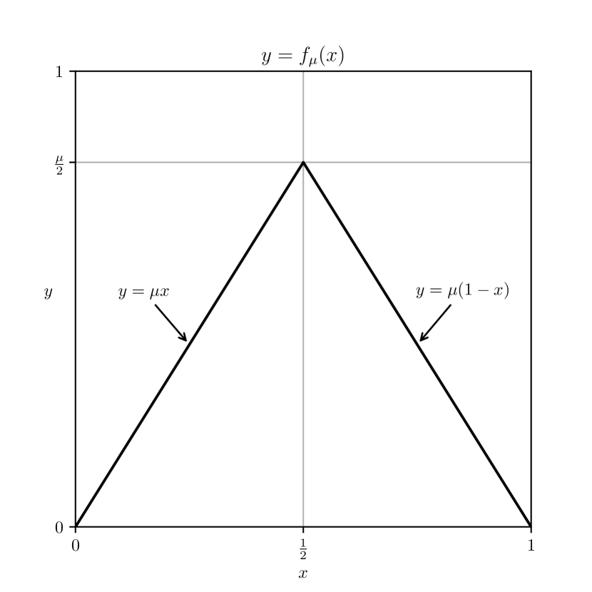
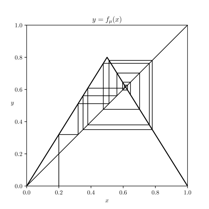
(a) Tent map $f(x)$ for $\mu=1.6$.

(b) Cobweb of $x_{0},x_{1},\ldots,x_{15}$ for $x_{0}=0.2$. Is $x_{1000}<\frac{1}{2}$?

Figure 1: A tent map $f(x)$ and its cobweb.

1.1 Background

Chaos.

Chaotic sequences show many interesting figures such as cobweb, strange attractor, bifurcation, etc. [22, 21, 24, 23, 18]. The chaos theory has been intensively developed in several context such as electrical engineering, information theory, statistical physics, neuroscience and computer science, with many applications, such as weather forecasting, climate change, diastrophism and disaster resilience since the 1960s. For instance, a cellular automaton, including the life game, is a classical topic in computer science, and it is closely related to the “edge of chaos.” For another instance, the “sensitivity to initial conditions” are often regarded as unpredictability, and chaotic sequences are used in pseudo random number generator, cryptography, or heuristics for NP-hard problems including chaotic genetic algorithms.

From the viewpoint of theoretical computer science, the numerical issues of computing chaotic sequences have been intensively investigated in statistical physics, information theory and probability. In contrast, the computational complexity of computing a chaotic sequence seems not well developed. It may be a simple reason that it looks unlike a decision problem.

Tent map: 1-D, piecewise-linear and chaotic.

Interestingly, very simple maps show chaotic behavior. One of the most simplest maps are piece-wise linear maps, including the tent map and the $\beta$-expansion (a.k.a. Bernoulli shift) which are 1-D maps and the baker’s map which is a 2-D map [22, 30, 26, 27, 31, 37, 6, 13, 29].

The tent map, as well as the $\beta$-expansion, is known to be topologically conjugate to the logistic map which is a quadratic map cerebrated as a chaotic map. Chaotic behavior of the tent map, in terms of power spectra, band structure, critical behavior, are analyzed in e.g., [22, 31, 37, 6]. The tent map is also used for pseudo random generator or encryption e.g., [1, 2, 20]. It is also used for meta-heuristics for NP-hard problems [35, 10].

Smoothed analysis.

Linear programming is an optimization problem on a (piecewise) linear system, for a linear objective function. Dantzig in 1947 gave an “efficient” algorithm, known as the simplex method, for linear programming. Khachiyan [17] gave the ellipsoid method, and proved that the linear programming is in P (cf. [19]) in 1979. Karmarkar [15] in 1984 gave another polynomial time algorithm, interior point method.

The smoothed analysis is introduced by Spielman and Teng [33], to prove that the simplex algorithms for linear programmings run in “polynomial time,” beyond the average case analysis. There are several recent progress on the smoothed analysis of algorithms [5, 4, 12, 11].

1.2 Contribution

This work.

This paper is concerned with a problem related to deciding whether $f^{n}(x)<1/2$ for $x\in[0,1)$ for the $n$-th iterated tent map $f^{n}$. More precisely, we will define the tent language ${\cal L}_{n}\subseteq\{0,1\}^{n}$ consisting of tent codes of $x\in[0,1)$ in Section 2, and we are concerned with the correct recognition of ${\cal L}_{n}$. The main target of the paper is the space complexity of the following simple problem; given a bit sequence $\mathbf{b}\in\{0,1\}^{n}$ and $x\in[0,1)$, decide whether $\mathbf{b}$ is a tent code of $x$. One may think that it is a problem just to compute $f^{i}(x)$ ($i=1,\ldots,n$), and there is nothing more than the precision issue, even in the sense of computational complexity. However, we will show in Section 2.2 that a standard calculation attended by rounding-off easily allows impossible tent code.

By a standard argument on the numerical error, cf. [19], $\mathrm{O}(n)$ space is enough to get it. At the same time, it seems hopeless to solve the target problem exactly in $\mathrm{o}(n)$ space, due to the “sensitivity to initial conditions” of a chaotic sequence. Then, this paper is concerned with a decision problem of whether an input $\mathbf{b}\in\{0,1\}^{n}$ is a tent code of $\epsilon$-perturbed $x$, and proves that it is correctly recognized in $\mathrm{O}(\log^{2}n)$ space (Theorem 2.8).

Related works.

The analysis technique of the paper basically follows [25], which showed that the recognition of ${\cal L}_{n}$ is in $\mathrm{O}(\log^{2}n)$ space in average. The technique is also very similar to or essentially the same as Markov extension developed in the context of symbolic dynamics. In 1979, Hofbauer [14] gave a representation of the kneading invariants for unimodal maps, which is known as the Markov extension and/or Hofbauer tower, and then discussed topological entropy. Hofbauer and Keller extensively developed the arguments in 1980s, see e.g., [7, 3]. We do not think the algorithms of the paper are trivial, but they are composed of the combination of the above nontrivial argument, and some classical techniques of designing space efficient algorithms.

As we stated above, the computational complexity of computing a chaotic sequence seems not well developed. Perl showed some NP-complete systems, e.g., knapsack, shows chaotic behavior [28]. On the other hand, it seems not known whether every chaotic sequence is hard to compute in the sense of NP-hard; particularly we are not sure if the problem $f^{n}(x)<1/2$ is NP-hard for a tent map $f$. Recently, chaotic dynamics are used for solving NP-hard problems e.g., SAT [8].

1.3 Organization

In Section 2, we will define the tent code, describe the issue of a standard calculation rounding-off, and show the precise results of the paper. Section 3 imports some basic technologies from [25]. Section 4 gives a simple algorithm for a valid calculation, as a preliminary step. Section 5 gives a smoothed analysis for the decision problem.

2 Issues and Results

2.1 Tent code

We define a tent-encoding function $\gamma^{n}_{\mu}\colon[0,1)\to\{0,1\}^{n}$ (or simply $\gamma^{n}$) as follows. For convenience, let $x_{i}=f^{i}(x)$ for $i=1,2,\ldots$ as given $x\in[0,1)$, where $f^{i}$ denote the $i$-times iterated tent map formally given by $f^{i}(x)=f(f^{i-1}(x))$ recursively. Then, the tent code $\gamma^{n}(x)=b_{1}\cdots b_{n}$ for $x\in[0,1)$ is a bit-sequence, where

$$b_{1} =\begin{cases}0&:x<\frac{1}{2},\\ 1&:x\geq\frac{1}{2},\end{cases}$$ (2)

and $b_{i}$ ($i=2,3,\ldots,n$) is recursively given by

$$b_{i+1} =\begin{cases}b_{i}&:x_{i}<\frac{1}{2},\\ \overline{b_{i}}&:x_{i}>\frac{1}{2},\\ 1&:x_{i}=\frac{1}{2},\end{cases}$$ (3)

where $\overline{b}$ denotes bit inversion of $b$, i.e., $\overline{0}=1$ and $\overline{1}=0$. We remark that the definition (3) is rephrased by

$$b_{i+1} =\begin{cases}0&:[b_{i}=0]\wedge\left[x_{i}<\frac{1}{2}\right],\\ 1&:[b_{i}=0]\wedge\left[x_{i}\geq\frac{1}{2}\right],\\ 1&:[b_{i}=1]\wedge\left[x_{i}\leq\frac{1}{2}\right],\\ 0&:[b_{i}=1]\wedge\left[x_{i}>\frac{1}{2}\right].\end{cases}$$ (4)

Proposition 2.1.

Suppose $\gamma_{\mu}^{\infty}(x)=b_{1}b_{2}\cdots$ for $x\in[0,1)$. Then, $(\mu-1)\sum_{i=1}^{\infty}b_{i}\mu^{-i}=x$.

See [25] for a proof. The proofs are not difficult but lengthy. Thanks to this a little bit artificial definition (3), we obtain the following two more facts.

Proposition 2.2.

For any $x,x^{\prime}\in[0,1)$,

$$x\leq x^{\prime} \Rightarrow\gamma_{\mu}^{n}(x)\preceq\gamma_{\mu}^{n}(x^{\prime})$$

hold where $\preceq$ denotes the lexicographic order, that is $b_{i_{*}}=0$ and $b^{\prime}_{i_{*}}=1$ at $i_{*}=\min\{j\in\{1,2,\ldots\}\mid b_{j}\neq b^{\prime}_{j}\}$ for $\gamma^{n}(x)=b_{1}b_{2}\cdots b_{n}$ and $\gamma^{n}(x^{\prime})=b^{\prime}_{1}b^{\prime}_{2}\cdots b^{\prime}_{n}$ unless $\gamma^{n}(x)=\gamma^{n}(x^{\prime})$.

Proposition 2.3.

The $n$-th iterated tent code is right continuous, i.e., $\gamma_{\mu}^{n}(x)=\gamma_{\mu}^{n}(x+0)$.

These two facts make the arguments simple. The following technical lemmas are useful to prove Propositions 2.2 and 2.3, as well as the arguments in Sections 4 and 5.

Lemma 2.4.

Suppose $x,x^{\prime}\in[0,1)$ satisfy $x<x^{\prime}$. If $\gamma^{n}(x)=\gamma^{n}(x^{\prime})$ then

$$\begin{cases}x_{n}<x^{\prime}_{n}&\mbox{if $b_{n}=b^{\prime}_{n}=0$, }\\ x_{n}>x^{\prime}_{n}&\mbox{if $b_{n}=b^{\prime}_{n}=1$}\end{cases}$$ (5)

holds.

Lemma 2.5.

If $\gamma^{n}(x)=\gamma^{n}(x^{\prime})$ for $x,x^{\prime}\in[0,1)$ then $|f^{n}(x)-f^{n}(x^{\prime})|=\mu^{n}|x-x^{\prime}|$.

Let ${\cal L}_{n,\mu}$ (or simply ${\cal L}_{n}$) denote the set of all $n$-bits tent codes, i.e.,

$${\cal L}_{n}=\left\{\gamma_{\mu}^{n}(x)\in\{0,1\}^{n}\ \middle|\ x\in[0,1)\right\}$$ (6)

and we call ${\cal L}_{n}$ tent language (by $\mu\in(1,2)$). Note that ${\cal L}_{n}\subsetneq\{0,1\}^{n}$ for $\mu\in(1,2)$. We say $\mathbf{b}_{n}\in\{0,1\}^{n}$ is a valid tent code if $\mathbf{b}_{n}\in{\cal L}_{n}$.

2.2 What is the issue?

A natural problem for the tent code could be calculation: given $x\in(0,1]$ and $n\in\mathbb{Z}_{>0}$, find $\gamma^{n}(x)$. By a standard argument (see e.g., [19]), it requires $\Theta(n\log\mu)$ working space to compute $f^{n}(x)$, in general. Thus, it is natural in practice to employ rounding-off, like Algorithm 1.

Algorithm 1 Rounding-off could output an invalid code

0:  $x\in[0,1]$

0:  a bit sequence $b_{1}\cdots b_{n}$ /* $b_{1}\cdots b_{n}\not\in{\cal L}_{n}$ in bad cases */

1:  set int $\kappa$ large constant

2:  rational $z\leftarrow\langle x\rangle_{\kappa}$ /* Round off by $\kappa$ bits (or digits) */

3:  bit $b\leftarrow 0$

4:  for $i=1$ to $n$ do

5:     if $b=0$ then

6:        if $z<\frac{1}{2}$ then $b\leftarrow 0$, else $b\leftarrow 1$/* recall (4) */

7:     else

8:        if $z>\frac{1}{2}$ then $b\leftarrow 0$, else $b\leftarrow 1$/* recall (4) */

9:     end if

10:     return  $b$ /* as $b_{i}$ */

11:     $z\leftarrow\langle f(z)\rangle_{\kappa}$

12:  end for

Due to the sensitivity to initial condition of a chaotic sequence, we cannot expect that Algorithm 1 to output $b_{1}\cdots b_{n}=\gamma^{n}(x)$ exactly, but we hope that it would output some approximation. It could be a natural question whether the output $b_{1}\cdots b_{n}\in{\cal L}_{n}$. The following proposition means that Algorithm 1 could output an impossible tent code.

Proposition 2.6.

Algorithm 1 could output $b_{1}\cdots b_{n}\not\in{\cal L}_{n}$.

Proof.

Let $\mu=1.62$, which is slightly greater than the golden ratio $\frac{1+\sqrt{5}}{2}\simeq 1.61803\ldots$, where the golden ratio is a solution of $\mu^{2}-\mu-1=0$. By our calculation, $\gamma_{\mu}^{15}(\frac{1}{2})=100\,011\,011\,011\,011$, and it is, of course, a word in ${\cal L}_{15}$. If we set $\langle z\rangle_{8}=\frac{\lfloor 2^{8}z\rfloor}{2^{8}}$, meaning that round down the nearest to $2^{-9}$, then Algorithm 1 outputs $100\,011\,011\,011\,00$, which is not a word of ${\cal L}_{14}$. Similarly for the same $\mu$, if we set $\langle z\rangle=\frac{\lfloor 1000z\rfloor}{1000}$, meaning that round down the nearest to $10^{-3}$, then Algorithm 1 outputs $100\,011\,011\,011\,010$, which is not a word of ${\cal L}_{15}$. ∎

Proposition 2.6 might not be surprising. Can we correct Algorithm 1 so as to output $b_{1}\dots b_{n}\in{\cal L}_{n}$? Yes it is possible if we set $\kappa=\Theta(n)$, that is sufficiently precise. Clearly, it requires $\Theta(n)$ working space. Then, it is validate to ask if it is possible to generate/recognize $b_{1}\dots b_{n}\in{\cal L}_{n}$ in $\mathrm{o}(n)$.

2.3 Problems and Results

The following problems could be natural in the sense of computational complexity of tent codes.

Problem 1 (Decision).

Given a real $x\in[0,1)$ and a bit sequence $\mathbf{b}_{n}\in\{0,1\}^{n}$, decide if $\mathbf{b}_{n}=\gamma^{n}(x)$.

Problem 2 (Calculation).

Given a real $x\in[0,1)$ and a positive integer $n$, find $\gamma^{n}(x)\in\{0,1\}^{n}$.

Recalling Proposition 2.6, it seems difficult to solve Problems 1 and 2 exactly, in $\mathrm{o}(n)$ space. Then, we consider to compute a valid tent code around $x$. Let $0<\epsilon\ll 1$, we define

$${\cal L}_{n}(x,\epsilon) =\{\gamma^{n}(x^{\prime})\mid x-\epsilon\leq x^{\prime}\leq x+\epsilon\}$$

for $x\in[0,1)$. It is equivalently rephrased by

$${\cal L}_{n}(x,\epsilon) =\{\mathbf{b}\in{\cal L}_{n}\mid\gamma^{n}(x-\epsilon)\preceq\mathbf{b}\preceq\gamma^{n}(x+\epsilon)\}$$ (7)

by Propositions 2.1 and 2.2. For the calculation Problem 2, we establish the following simple theorem.

Theorem 2.7 (Approximate calculation).

Let $\mu\in(1,2)$ be rational given by an irreducible fraction $\mu=c/d$, and let $0<\epsilon<1/4$. Given a real $x\in[0,1)$, Algorithm 2 described in Section 4 outputs $\mathbf{b}_{n}\in{\cal L}_{n}(x,\epsilon)$. The space complexity of Algorithm 2 is $\mathrm{O}(\lg^{2}\epsilon^{-1}\lg d/\lg^{2}\mu+\lg n)$.

Then, the following theorem for Problem 1 is the main result of the paper.

Theorem 2.8 (Decision for $\epsilon$-perturbed input).

Let $\mu\in(1,2)$ be rational given by an irreducible fraction $\mu=c/d$, and let $0<\epsilon<1/4$. Given a bit sequence $\mathbf{b}_{n}\in\{0,1\}^{n}$ and a real $x\in[0,1)$, Algorithm 3 described in Section 5 accepts it if $\mathbf{b}_{n}\in{\cal L}_{n}(x,\epsilon)$ and rejects it if $\mathbf{b}_{n}\not\in{\cal L}_{n}(x,2\epsilon)$. If an ($\epsilon$-perturbed) instance $\mathbf{b}_{n}$ is given by $\mathbf{b}_{n}=\gamma^{n}(X)$ for $X\in[x-\epsilon,x+\epsilon]$ uniformly at random then the space complexity of Algorithm 3 is $\mathrm{O}(\lg^{2}n/\lg^{3}d+\lg\epsilon^{-1}/\lg d)$ in expectation.

As stated in theorems, this paper assumes $\mu$ rational mainly for the reason of Turing comparability, but it is not essential. Instead, we allow an input instance $x\in[0,1)$ being a real, given by a read only tape of infinite length. We remark that the space complexity of Theorem 2.7 is optimal in terms of $n$.

Proof strategy of the theorems.

For proofs, we will introduce the “automaton” for ${\cal L}_{n}$ given by [25] in Section 3. Once we get the automaton, Theorem 2.7 is not difficult, and we prove it in Section 4. Algorithm 2 is relatively simple and the space complexity is trivial. Thus, the correctness is the issue, but it is also not very difficult. Then, we give Algorithm 3 and prove Theorem 2.8 in Section 5. The correctness is essentially the same as Algorithm 2. The analysis of the space complexity is the major issue.

3 Underlying Technology

This section briefly introduces some fundamental technology for the analyses in Sections 4 and 5 including the automaton and the Markov chain for ${\cal L}_{n}$, according to [25].

The key idea of a space efficient computation of a tent code is a representation of an equivalent class with respect to $\gamma^{n}$. Let

$$T(\mathbf{b}_{n}) \overset{\rm def}{=}\{f^{n}(x)\mid\gamma^{n}(x)=\mathbf{b}_{n}\}$$ (8)

for $\mathbf{b}_{n}\in{\cal L}_{n}$, we call $T(\mathbf{b}_{n})$ the segment-type of $\mathbf{b}_{n}$. In fact, $T(\mathbf{b}_{n})$ is a continuous interval, where one end is open and the other is close. By some straightforward argument with (4), we get the following recursive formula.

Lemma 3.1 ([25]).

Let $x\in[0,1)$, and let $\gamma^{n}(x)=b_{1}\cdots b_{n}$.
(1) Suppose $T^{i}(x)=[v,u)$ ($v<u$).

• $v<\frac{1}{2}<u$.

  • If $f^{i}(x)<1/2$ then $T^{i+1}(x)=[f(v),f(\tfrac{1}{2}))$, and $b_{i+1}=0$.

  • If $f^{i}(x)\geq 1/2$ then $T^{i+1}(x)=(f(u),f(\tfrac{1}{2})]$, and $b_{i+1}=1$.

• $u\leq\frac{1}{2}$. Then $T^{i+1}(x)=[f(v),f(u))$, and $b_{i+1}=0$.

• $v\geq\frac{1}{2}$. Then $T^{i+1}(x)=(f(u),f(v)]$, and $b_{i+1}=1$.

(2) Similarly, suppose $T^{i}(x)=(v,u]$ ($v<u$).

• $v<\frac{1}{2}<u$.

  • If $f^{n}(x)\leq 1/2$ then $T^{i+1}(x)=(f(v),f(\tfrac{1}{2})]$, and $b_{i+1}=1$.

  • If $f^{n}(x)>1/2$ then $T^{i+1}(x)=[f(u),f(\tfrac{1}{2}))$, and $b_{i+1}=0$.

• $u\leq\frac{1}{2}$. Then $T^{i+1}(x)=(f(v),f(u)]$, and $b_{i+1}=1$.

• $v\geq\frac{1}{2}$. Then $T^{i+1}(x)=[f(u),f(l))$, and $b_{i+1}=0$.

Let

$$\mathcal{T}_{n}=\{T(\mathbf{b})\subseteq[0,1)\mid\mathbf{b}\in{\cal L}_{n}\}$$ (9)

denote the set of segment-types (of ${\cal L}_{n}$). It is easy to observe that $|{\cal L}_{n}|$ can grow exponential to $n$, while the following theorem implies that $|\mathcal{T}_{n}|\leq 2n$.

Theorem 3.2 ([25]).

Let $\mu\in(1,2)$. Let $\mathbf{c}_{i}=\gamma^{i}(\frac{1}{2})$, and let

$$I_{i}=T(\mathbf{c}_{i})\hskip 20.00003pt\mbox{and}\hskip 20.00003pt\overline{I}_{i}=T(\overline{\mathbf{c}}_{i})$$ (10)

for $i=1,2,\ldots$. Then,

$$\mathcal{T}_{n}=\bigcup_{i=1}^{n_{*}}\left\{I_{i},\overline{I}_{i}\right\}$$

for $n\geq 1$, where $n_{*}=\min(\{i\in\{1,2,\ldots,n-1\}\mid I_{i+1}\in\mathcal{T}_{i}\}\cup\{n\})$.

The following lemma, derived from Lemma 3.1, gives an explicit recursive formula of $I_{i}$ and $\overline{I}_{i}$.

Lemma 3.3 ([25]).

$I_{i}$ and $\overline{I}_{i}$ given by (10) are recursively calculated for $i=1,2,\ldots$ as follows.

$$I_{1}=[0,\tfrac{\mu}{2})\hskip 20.00003pt\mbox{and}\hskip 20.00003pt\overline{I}_{1}=(0,\tfrac{\mu}{2}].$$

For $i=2,3,\ldots$,

$$I_{i} =\begin{cases}\begin{cases}[f(v),f(\tfrac{1}{2}))&:v<\tfrac{1}{2}<u\\ [f(v),f(u))&:u\leq\tfrac{1}{2}\\ (f(u),f(v)]&:v\geq\tfrac{1}{2}\end{cases}&\mbox{if $I_{i-1}=[v,u)$, }\\ \begin{cases}[f(u),f(\tfrac{1}{2}))&:v<\tfrac{1}{2}<u\\ (f(v),f(u)]&:u\leq\tfrac{1}{2}\\ [f(u),f(v))&:v\geq\tfrac{1}{2}\end{cases}&\mbox{if $I_{i-1}=(v,u]$}\end{cases}$$ (11)

holds. Then,

$$\overline{I}_{i} =\begin{cases}(v,u]&\mbox{if $I_{i}=[v,u)$}\\ [v,u)&\mbox{if $I_{i}=(v,u]$}\end{cases}$$

holds.

For convenience, we define the level of $J\in\mathcal{T}_{n}$ by

$$L(J)=k$$ (12)

if $J=I_{k}$ or $\overline{I_{k}}$. Notice that Theorem 3.2 implies that the level of $T(\mathbf{b}_{k})$ for $\mathbf{b}_{k}\in{\cal L}_{k}$ may be strictly less than $k$. In fact, it happens, which provides a space efficient “automaton”.

Figure 2: Transition diagram over $\mathcal{T}_{n}$ for $\mu=1.6$.

State transit machine (“automaton”).

By Theorem 3.2, we can design a space efficient state transit machine according to Lemma 3.1, to recognize ${\cal L}_{n}$. We define the set of states by $Q_{n}=\{q_{0}\}\cup\{\emptyset\}\cup\mathcal{T}_{n}$, where $q_{0}$ is the initial state, and $\emptyset$ denotes the unique reject state. Let $\delta\colon Q_{n-1}\times\{0,1\}\to Q_{n}$ denote the state transition function, defined as follows. Let $\delta(q_{0},1)=I_{1}$ and $\delta(q_{0},0)=\overline{I}_{1}$. According to Lemma 3.1, we appropriately define

$$\delta(J,b)=J^{\prime}$$ (13)

for $J\in\mathcal{T}_{n-1}$ and $b\in\{0,1\}$, as far as $J$ and $b$ are consistent. If the pair $J$ and $b$ are inconsistent, we define $\delta(J,b)=\emptyset$; precisely

$$\begin{cases}\mbox{$J=(v,u]$ and $v\geq\frac{1}{2}$}&\mbox{(cf. Case 1-3)}\\ \mbox{$J=[v,u)$ and $u\leq\frac{1}{2}$}&\mbox{(cf. Case 2-2)}\\ \mbox{$J=[v,u)$ and $u\leq\frac{1}{2}$}&\mbox{(cf. Case 1-2)}\\ \mbox{$J=(v,u]$ and $v\geq\frac{1}{2}$}&\mbox{(cf. Case 2-3)}\end{cases}$$

are the cases, where $v=\inf J$ and $u=\sup J$.

Lemma 3.4 ([25]).

Let $\mu\in(1,2)$ be a rational given by an irreducible fraction $\mu=c/d$. For any $k\in\mathbb{Z}_{>0}$, the state transit machine on $Q_{k}$ is represented by $\mathrm{O}(k^{2}\lg{d})$ bits.

We will use the following two technical lemmas about the transition function in Sections 4 and 5.

Lemma 3.5 ([25]).

Suppose for $\mu\in(1,2)$ that $f_{\mu}^{i}(\frac{1}{2})\neq\frac{1}{2}$ holds for any $i=1,\dots,n-1$. Then,

$$\delta(I_{n},b) \in\left\{I_{n+1}\right\}\cup\left\{\overline{I}_{k+1}\mid 1\leq k\leq\tfrac{n}{2}\right\}\cup\{\emptyset\}$$

hold for $b=0,1$.

Lemma 3.6 ([25]).

Suppose for $\mu\in(1,2)$ that $f_{\mu}^{i}(\frac{1}{2})\neq\frac{1}{2}$ holds for any $i=1,\dots,2n-1$. Then, there exists $k\in\{n+1,\ldots,2n\}$ and $b\in\{0,1\}$ such that

$$\delta(I_{k},b) \in\left\{\overline{I}_{k^{\prime}+1}\mid 1\leq k^{\prime}\leq\tfrac{k}{2}\right\}$$

hold.

Roughly speaking, Lemma 3.5 implies that the level increases by one, or decreases into (almost) a half by a transition step. Furthermore, Lemma 3.6 implies that there is at least one way to decrease the level during $n,\ldots,2n$.

Markov model.

Furthermore, the state transitions preserve the uniform measure, over $[0,1)$ in the beginning, since the tent map is piecewise linear.

Lemma 3.7 ([25]).

Let $X$ be a random variable drawn from $[0,1)$ uniformly at random. Let $\mathbf{b}_{n}\in{\cal L}_{n}$. Then,

$$\Pr[B_{n+1}=b\mid\gamma^{n}(X)=\mathbf{b}_{n}]=\frac{|T(\mathbf{b}_{n}b)|}{|T(\mathbf{b}_{n}0)|+|T(\mathbf{b}_{n}1)|}$$

holds for $b\in\{0,1\}$, where let $|T(\mathbf{b}_{n}b)|=0$ if $\mathbf{b}_{n}b\not\in{\cal L}_{n+1}$.

Let ${\cal D}_{n,\mu}$ (or simply ${\cal D}_{n}$) denote a probability distribution over ${\cal L}_{n}$ which follows $\gamma^{n}(X)$ for $X$ is uniformly distributed over $[0,1)$, i.e., ${\cal D}_{n}$ represents the probability of appearing $\mathbf{b}_{n}\in{\cal L}_{n}$ as given the initial condition $x$ uniformly at random.

Theorem 3.8 ([25]).

Let $\mu\in(1,2)$ be a rational given by an irreducible fraction $\mu=c/d$. Then, it is possible to generate $B\in{\cal L}_{n}$ according to ${\cal D}_{n}$ in $\mathrm{O}(\lg^{2}n\lg^{3}d/\lg^{4}\mu)$ space in expectation (as well as, with high probability).

Thus, we remark that the tent language ${\cal L}_{n}$ is recognized in $\mathrm{O}(\lg^{2}n\lg^{3}d/\lg^{4}\mu)$ space on average all over the initial condition $x\in[0,1)$, by Theorem 3.8.

4 Calculation in “Constant” Space

Theorem 2.7 is easy, once the argument in Section 3 is accepted. Algorithm 2 shows the approximate calculation of $\gamma^{n}(x)$ so that the output is a valid tent code (recall the issue in Section 2.2). Roughly speaking, Algorithm 2 calculates by rounding-off to $\kappa=\mathrm{O}(\log\epsilon^{-1})$ bits for the first $\kappa$ iterations (lines 5–10), and then traces the automaton within the level $2\kappa$ after the $\kappa$-th iteration (lines 11–20). The algorithm traces finite automaton, and the desired space complexity is almost trivial. A main issue is the correctness; it is also trivial that the output sequence $\mathbf{b}_{n}\in\{0,1\}^{n}$ is a valid tent code, then our goal is to prove $\gamma^{n}(x-\epsilon)\preceq\mathbf{b}_{n}\preceq\gamma^{n}(x+\epsilon)$. The trick is based on the fact that the tent map is an extension map, which will be used again in the smoothed analysis in the next session.

Then we explain the detail of Algorithm 2. Let $\langle x\rangle_{k}$ denote a binary expression by the rounding off a real $x$ to the nearest $1/2^{k+1}$, where the following argument only requires $|\langle x\rangle_{k}-x|\leq 1/2^{k}$, meaning that rounding up and down is not essential. Naturally assume that $\langle x\rangle_{k}$ for $x\in[0,1)$ is represented by $k$ bits, meaning that the space complexity of $\langle x\rangle_{k}$ is $\mathrm{O}(k)$.

In the algorithm, rationals $v[k]$ and $u[k]$ respectively denote $\inf I_{k}$ and $\sup I_{k}$ for $k=1,2,\ldots$. For descriptive purposes, $v[0]$ and $u[0]$ corresponds to $q_{0}$, and $v[-1]$ and $u[-1]$ corresponds to the reject state $\emptyset$ in $Q_{n}$. The single bit $c[k]$ denotes $c_{k}$ for $\mathbf{c}_{n}=c_{1}\cdots c_{n}=\gamma^{n}(\frac{1}{2})$ (recall Theorem 3.2). Thus, $I_{k}=[v[k],u[k])$ and $\overline{I}_{k}=(v[k],u[k]]$ if $c[k]=0$, otherwise $I_{k}=(v[k],u[k]]$ and $\overline{I}_{k}=[v[k],u[k])$ see Section 3. The integer $\delta(l,b)=l^{\prime}$ represents the transition $\delta(I_{l},b)=J^{\prime}$, where $J^{\prime}=I_{l^{\prime}}$ or $\overline{I}_{l^{\prime}}$, given by (13) in Section 3. Notice that if $\delta(I_{l},b)=J^{\prime}$ then $\delta(\overline{I}_{l},b)=\overline{J^{\prime}}$ holds [25]. The pair $l$ and $b$ represent $Z_{i}=I_{l}$ if $b=c[l]$, otherwise, i.e., $\overline{b}=c[l]$, $Z_{i}=\overline{I}_{l}$, at the $i$-th iteration (for $i=1,\ldots n$). See Section A for the detail of the subprocesses, Algorithms 4 and 5.

Algorithm 2 Valid calculation with “constant” space (for $\mu,\epsilon$)

0:  a real $x\in[0,1]$

0:  a bit sequence $b_{1}\cdots b_{n}\in{\cal L}_{n}(x,\epsilon)$

1:  int $\kappa\leftarrow\lceil-3\lg\epsilon/\lg\mu\rceil$

2:  compute rational $v[k]$, rational $u[k]$, bit $c[k]$, int $\delta[k,0]$ and int $\delta[k,1]$ for $k=-1$ to $2\kappa$ by Algorithm 4

3:  int $l\leftarrow 0$, bit $b\leftarrow 1$

4:  rational $z\leftarrow\langle x\rangle_{\kappa}$

5:  for $i=1$ to $\kappa$ do

6:     compute bit $b^{\prime}$ based on $b$ and $z$ by (4)

7:     return  $b^{\prime}$ /* as $b_{i}$ */

8:     update $l$ based on $b$ and $b^{\prime}$, update $b$ (by Algorithm 5)

9:     $z\leftarrow\langle f(z)\rangle_{\kappa}$

10:  end for

11:  for $i=\kappa+1$ to $n$ do

12:     $b^{\prime}\leftarrow\arg\min\{\delta(l,b^{\prime\prime})\mid b^{\prime\prime}\in\{0,1\},\ \delta(l,b^{\prime\prime})>0\}$

13:     if $b=c[l]$ then

14:        $b\leftarrow b^{\prime}$

15:     else

16:        $b\leftarrow\overline{b^{\prime}}$

17:     end if

18:     return  $b$ /* as $b_{i}$ */

19:     $l\leftarrow\delta[l,b^{\prime}]$

20:  end for

Theorem 4.1 (Theorem 2.7).

Given a real $x\in[0,1)$, Algorithm 2 outputs $\mathbf{b}_{n}\in{\cal L}_{n}(x,\epsilon)$. The space complexity of Algorithm 2 is $\mathrm{O}(\lg^{2}\epsilon^{-1}\lg d/\lg^{2}\mu+\lg n)$.

Proof.

To begin with, we remark that Algorithm 2 constructs the transition diagram only up to the level $2\kappa$. Nevertheless, Algorithm 2 correctly conducts the for-loop in lines 11–20, meaning that all transitions at line 19 are always valid during the loop. This is due to Lemma 3.6, which claims that there exists at least one $l\in\{\kappa+1,\ldots,2\kappa\}$ such that $\delta(l,b)\leq\kappa$ (and also $\delta(l,b)>0$), meaning that it is a reverse edge. Then, it is easy from Lemma 3.4 that the space complexity of Algorithm 2 is $\mathrm{O}(\kappa^{2}\lg d)=\mathrm{O}(\lg^{2}\epsilon\lg d/\lg^{2}\mu)$, except for the space $\mathrm{O}(\lg n)$ of counter $i$ (and $n$) at line 11.

Then, we prove $b_{1}\cdots b_{n}\in{\cal L}_{n}(x,\epsilon)$. Since the algorithm follows the transition diagram of ${\cal L}_{n}$ (recall Section 3), it is easy to see that $b_{1}\cdots b_{n}\in{\cal L}_{n}$, and hence we only need to prove

$$\gamma^{n}(x-\epsilon)\preceq b_{1}\cdots b_{n}\preceq\gamma^{n}(x+\epsilon)$$ (14)

holds. We here only prove $\gamma^{n}(x-\epsilon)\preceq b_{1}\cdots b_{n}$ while $b_{1}\cdots b_{n}\preceq\gamma^{n}(x+\epsilon)$ is essentially the same. The proof is similar to that of Proposition 2.2, while the major issue is whether rounding $\langle z\rangle_{\kappa}$ preserves the “ordering,” so does the exact calculation by Lemma 2.4.

For convenience, let $z_{i}$ denote the value of $z$ in the $i$-th iteration of the algorithm, i.e., $z_{i+1}=\langle f(z_{i})\rangle_{\kappa}$. Let $x^{-}=x-\epsilon/2$ and let $x^{--}=x-\epsilon$. The proof consists of two parts:

$$\gamma^{\kappa}(x^{--}) \prec\gamma^{\kappa}(x^{-})\hskip 20.00003pt\mbox{and}$$ (15)

$$\gamma^{\kappa}(x^{-}) \preceq b_{1}\cdots b_{\kappa}.$$ (16)

For the claim (15), notice that $\gamma^{\kappa}(x^{--})\preceq\gamma^{\kappa}(x^{-})$ by Lemma 2.4. If $\gamma^{\kappa}(x^{--})=\gamma^{\kappa}(x^{-})$, Lemma 2.5 implies that $|f^{\kappa}(x^{--})-f^{\kappa}(x^{-})|=\frac{\epsilon}{2}\mu^{\kappa}\geq\frac{\epsilon}{2}\mu^{-3\lg\epsilon/\lg\mu}=\frac{1}{2\epsilon^{2}}>1$, which contradicts to $0\leq f^{\kappa}(x^{\prime})\leq 1$ for any $x^{\prime}\in[0,1)$. Now we get (15).

For (16), similar to the proof of Proposition 2.2 based on Lemma 2.4, we claim if $\gamma^{i}(x^{-})=b_{1}\cdots b_{i}$ then

$$\begin{cases}x^{-}_{i}<z_{i}&\mbox{if $b_{i}=0$, }\\ x^{-}_{i}>z_{i}&\mbox{if $b_{i}=1$}\end{cases}$$ (17)

hold. The basic argument is essentially the same as the proof of Lemma 2.4, which is based on the argument of segment type (see [25]), and here it is enough to check

if $$|x^{-}_{i}-z_{i}|\geq\frac{\epsilon}{2} |x^{-}_{i+1}-z_{i+1}|\geq\frac{\epsilon}{2} \gamma^{i+1}(x)=\gamma^{i+1}(z)$$ then , as far as (18)

meaning that the rounding-off does not disrupt the order. Notice that

$$|x^{-}_{i+1}-z_{i+1}| =|f(x^{-}_{i})-\langle f(z_{i})\rangle_{\kappa}|\geq|f(x^{-}_{i})-f(z_{i})|-|\langle f(z_{i})\rangle_{\kappa}-f(z_{i})|$$ (19)

holds, where the last inequality follows the triangle inequality $|f(x^{-}_{i})-\langle f(z_{i})\rangle_{\kappa}|+|\langle f(z_{i})\rangle_{\kappa}-f(z_{i})|\geq|f(x^{-}_{i})-f(z_{i})|$. Note that $|f(x^{-}_{i})-f(z_{i})|=\mu|x^{-}_{i}-z_{i}|\geq\mu\frac{\epsilon}{2}$ holds under the hypothesis $\gamma^{i+1}(x)=\gamma^{i+1}(z)$. We also remark $|\langle f(z_{i})\rangle_{\kappa}-f(z_{i})|\leq\frac{1}{2^{\kappa}}$ by definition of $\langle\cdot\rangle_{\kappa}$. Furthermore, we claim $\frac{1}{2^{\kappa}}\leq(\mu-1)\frac{\epsilon}{2}$ by $\kappa\geq-3\lg\epsilon/\lg\mu$: note that $1/\lg\mu\geq 0.7-\lg(\mu-1)$ holds for $1<\mu<2$, and then $\kappa\geq-3\lg\epsilon(0.7-\lg(\mu-1))=-2.1\lg\epsilon+3\lg\epsilon\lg(\mu-1)\geq-\lg\epsilon^{2}-\lg(\mu-1)\geq-\lg\frac{\epsilon}{2}-\lg(\mu-1)$ holds where we use $\epsilon<1/4$, which implies the desired claim $\frac{1}{2^{\kappa}}\leq(\mu-1)\frac{\epsilon}{2}$. Then,

$$\eqref{eq:20231029a}\geq\mu\tfrac{\epsilon}{2}-\tfrac{1}{2^{\kappa}}\geq\mu\tfrac{\epsilon}{2}-(\mu-1)\tfrac{\epsilon}{2}=\tfrac{\epsilon}{2},$$ (20)

and we got (18), and hence (16) by Proposition 2.2. By (15) and (16), $\gamma^{\kappa}(x-\epsilon)\preceq b_{1}\cdots b_{\kappa}$ is easy. Now, we obtain (14) by Proposition 2.2. ∎

5 Smoothed Analysis for Decision

Now, we are concerned with the decision problem, Problem 1. Algorithm 3 efficiently solves the problem with $\epsilon$-perturbed input, for Theorem 2.8. Roughly speaking, Algorithm 3 checks whether $\mathbf{b}_{n}\in{\cal L}_{n}$ at line 24, and checks whether $\gamma^{n}(x-\epsilon)\preceq\mathbf{b}_{n}\preceq\gamma^{n}(x+\epsilon)$ for lines 6–22. Lines 25–27 show a deferred update of those parameters, to save the space complexity.

Algorithm 3 Decision (for $\mu,\epsilon$)

0:  a bit sequence $b_{1}\cdots b_{n}\in\{0,1\}^{n}$ and a real $x\in[0,1]$

0:  Accept if $b_{1}\cdots b_{n}\in{\cal L}_{n}(x,\epsilon)$ and Reject if $b_{1}\cdots b_{n}\not\in{\cal L}_{n}(x,2\epsilon)$

1:  int $\kappa\leftarrow\lceil-3\lg\epsilon/\lg\mu\rceil$

2:  compute rational $v[k]$, rational $u[k]$, bit $c[k]$, int $\delta[k,0]$ and int $\delta[k,1]$ for $k=-1$ to $\kappa$ by Algorithm 4

3:  int $k\leftarrow\kappa$, int $l\leftarrow 0$, int ${\it case}\leftarrow 1$

4:  rational $z^{-}\leftarrow\langle x-\frac{3}{2}\epsilon\rangle_{\kappa}$, rational $z^{+}\leftarrow\langle x+\frac{3}{2}\epsilon\rangle_{\kappa}$

5:  for $i=1$ to $n$ do

6:     if ${\it case}=1$ then

7:        compute bit $b^{-}$, $b^{+}$ respectively based on $z^{-}$, $z^{+}$ with $b_{i-1}$ by (4)

8:        if $b_{i}<b^{-}$ or $b^{+}<b_{i}$ then return Reject and halt

9:        else if $b^{-}<b_{i}$ and $b_{i}=b^{+}$ then ${\rm case}\leftarrow 2$

10:        else if $b^{-}=b_{i}$ and $b_{i}<b^{+}$ then ${\rm case}\leftarrow 3$

11:        else $z^{-}\leftarrow\langle f(z^{-})\rangle_{\kappa}$, $z^{+}\leftarrow\langle f(z^{+})\rangle_{\kappa}$ /* i.e., $b_{-}=b_{+}=b_{i}$ */

12:     else if ${\it case}=2$ then

13:        compute bit $b^{+}$ based on $z^{+}$ with $b_{i-1}$ by (4)

14:        if $b^{+}<b_{i}$ then return Reject and halt

15:        else if $b_{i}<b^{+}$ then ${\rm case}\leftarrow 0$

16:        else $z^{+}\leftarrow\langle f(z^{+})\rangle_{\kappa}$ /* i.e., $b_{+}=b_{i}$ */

17:     else if ${\it case}=3$ then

18:        compute bit $b^{-}$ based on $z^{-}$ with $b_{i-1}$ by (4)

19:        if $b_{i}<b^{-}$ then return Reject and halt

20:        else if $b^{-}<b_{i}$ then ${\rm case}\leftarrow 0$

21:        else $z^{-}\leftarrow\langle f(z^{-})\rangle_{\kappa}$ /* i.e., $b_{-}=b_{i}$ */

22:     end if

23:     update $l$ based on $b_{i-1}$ and $b_{i}$ (by Algorithm 5)

24:     if $l=-1$ then return Reject and halt

25:     if $l=k$ then

26:        compute $v[k+1]$, $u[k+1]$, $c[k+1]$, $\delta[k,0]$ and $\delta[k,1]$ by Algorithm 4

27:     end if

28:  end for

29:  return  Accept

Theorem 5.1 (Theorem 2.8).

Given a bit sequence $\mathbf{b}_{n}\in\{0,1\}^{n}$ and a real $x\in[0,1)$, Algorithm 3 accepts it if $\mathbf{b}_{n}\in{\cal L}(x,\epsilon)$ and rejects it if $\mathbf{b}_{n}\not\in{\cal L}_{n}(x,2\epsilon)$. If an ($\epsilon$-perturbed) instance $\mathbf{b}_{n}$ is given by $\mathbf{b}_{n}=\gamma^{n}(X)$ for $X\in[x-\epsilon,x+\epsilon]$ uniformly at random then the space complexity of Algorithm 3 is $\mathrm{O}(\lg^{2}n/\lg^{3}d+\lg\epsilon^{-1}/\lg d)$ in expectation.

Proof.

The correctness proof is essentially the same as that of Theorem 2.7. In the algorithm, line 29 checks whether $b_{1}\cdots b_{n}\in{\cal L}_{n}$. We see whether $\gamma^{n}(x-\epsilon)\prec b_{1}\cdots b_{n}\prec\gamma^{n}(x+\epsilon)$ for the first at most $\kappa$ iterations, as follows. Let $b^{-}_{i}$ and $b^{+}_{i}$ respectively represent $b^{-}$ and $b^{+}$ computed at line 7, 13 or 18 of the $i$th iteration. Then, $b^{-}_{1}\cdots b^{-}_{\kappa}\prec\gamma^{\kappa}(x)\prec b^{+}_{1}\cdots b^{+}_{\kappa}$ hold, by the essentially same way as (15) in the proof of Theorem 2.7. Similarly, $\gamma^{\kappa}(x-\epsilon)\prec b^{-}_{1}\cdots b^{-}_{\kappa}$ holds, $b^{+}_{1}\cdots b^{+}_{\kappa}\prec\gamma^{\kappa}(x+\epsilon)$ as well. Thus, $\mathbf{b}_{n}\prec\gamma^{\kappa}(x-\epsilon)$ is safely rejected at line 8 or 19, $\gamma^{\kappa}(x+\epsilon)\prec\mathbf{b}_{n}$ as well at line 8 or 13. Thus we obtain the desired decision.

Then we are concerned with the space complexity. The analysis technique is very similar to or essentially the same as [25] for a random generation of ${\cal L}_{n}$. Let $X$ be a random variable drawn from the interval $[x-\epsilon,x+\epsilon]$ uniformly at random. Let $\gamma^{n}(X)=B_{1},$ Let

$$K=\max\{k\in\mathbb{Z}_{>0}\mid L(T(\gamma^{i}(X)))=k\}$$ (21)

be a random variable where $L(J)=k$ if $J=I_{k}$ or $\overline{I}_{k}$ (recall (12) as well as Theorem 3.2). Lemma 3.4 implies that its space complexity is $\mathrm{O}(K^{2}\lg{d})$. Lemma 5.2, appearing below, implies

$$\mathrm{E}[\mathrm{O}(K^{2}\lg{d})] =\mathrm{O}(\mathrm{E}[K^{2}]\lg{d})$$

$$=\mathrm{O}(\lg^{2}{n}\lg^{3}{d}/\lg^{4}\mu)$$

and we obtain the claim. ∎

Lemma 5.2.

Let $\mu\in(1,2)$ be rational given by an irreducible fraction $\mu=c/d$. Suppose for $\mu\in(1,2)$ that $f_{\mu}^{i}(\frac{1}{2})\neq\frac{1}{2}$ holds for any $i=1,\dots,n-1$. Then, $\mathrm{E}[K^{2}]=\mathrm{O}(\log_{\mu}^{2}{n}\log_{\mu}^{2}{d})=\mathrm{O}(\lg^{2}n\lg^{2}d/\lg^{4}\mu)$.

We remark that the assumption of rational $\mu$ is not essential in Lemma 5.2; the assumption is just for an argument about Turing comparability. We can establish a similar (but a bit weaker) version of Lemma 5.4 for any real $\mu\in(0,1)$ (cf. Proposition 5.1 of [25]). Lemma 5.2 is similar to Lemma 4.3 of [25] for random generation, where the major difference is that [25] assumes $X_{0}$ is uniform on $[0,1)$ while Lemma 5.2 here assumes $X_{0}$ is uniform on $[x-\epsilon,x+\epsilon]$. We only need to take care of some trouble when the initial condition is around the boundaries of the interval, $x-\epsilon$ and $x+\epsilon$.

Suppose for the proof of Lemma 5.2 that a random variable $X$ is drawn from the interval $[x-\epsilon,x+\epsilon]$ uniformly at random. Let $X_{0}=X$ and let $X_{i}=f(X_{i-1})$ for $i=1,2,\ldots,n$. For convenience, let $T^{i}(x)$ denote $T(\gamma^{i}(x))$. Let $y\in[x-\epsilon,x+\epsilon]$. We say $X$ covers around $y$ at $i$-th iteration ($i\in\{1,2,\ldots,n\}$) if

$$\{f^{i}(y^{\prime})\mid\gamma^{i}(y^{\prime})=\gamma^{i}(y),\,x-\epsilon\leq y^{\prime}\leq x+\epsilon\}=T^{i}(y)$$ (22)

holds (recall $T^{i}(y)=\{f^{i}(y^{\prime})\mid\gamma^{i}(y^{\prime})=\gamma^{i}(y)\}$ by definition 8). Similarly, we say $X$ fully covers $S$ ($S\subseteq[x-\epsilon,x+\epsilon]$) at $i\in\{1,2,\ldots,n\}$ if $X$ covers around every $y\in S$ at $i$.

Lemma 5.3.

$X$ fully covers $(x-\epsilon+\frac{1}{n^{2}},x+\epsilon-\frac{1}{n^{2}})$ at or after $\lceil 2\log_{\mu}n\rceil$ iterations.

Proof.

Let $k=\lceil 2\log_{\mu}n\rceil$. By Lemma 2.5, if $y,y^{\prime}\in[0,1)$ satisfies $\gamma^{k}(y)=\gamma^{k}(y^{\prime})$ then $|f^{k}(y)-f^{k}(y^{\prime})|=\mu^{k}|y-y^{\prime}|\geq\mu^{2\log_{\mu}n}|y-y^{\prime}|=n^{2}|y-y^{\prime}|$. On the other hand, $|f^{k}(y)-f^{k}(y^{\prime})|\leq 1$, and hence the claim is easy from Propositions 2.1 and 2.2. ∎

Then, the proof of Lemma 5.2 consists of two parts: one is that the conditional expectation of $K^{2}$ is $\mathrm{O}(\lg^{2}n\lg^{2}d/\lg^{4}\mu)$ on condition that $X\in(x-\epsilon+\frac{1}{n^{2}},x+\epsilon-\frac{1}{n^{2}})$ (Lemma 5.4), and the other is that the probability of $X\not\in(x-\epsilon+\frac{1}{n^{2}},x+\epsilon-\frac{1}{n^{2}})$ is small enough to allow Lemma 5.2 from Lemma 5.4. The latter claim is almost trivial (see the proof of Lemma 5.2 below)

The following lemma is the heart of the analysis, which is a version of Lemma 4.3 of [25] for random generation (see also Appendix B, for a proof).

Lemma 5.4.

Let $\mu\in(1,2)$ be rational given by an irreducible fraction $\mu=c/d$. Suppose for $\mu\in(1,2)$ that $f_{\mu}^{i}(\frac{1}{2})\neq\frac{1}{2}$ holds for any $i=1,\dots,n-1$. On condition that $X$ fully covers $(x-\epsilon+\frac{1}{n^{2}},x+\epsilon-\frac{1}{n^{2}})$ at $\lceil\log_{\mu}n\rceil$, the conditional expectation of $K^{2}$ is $\mathrm{O}(\log_{\mu}^{2}{n}\log_{\mu}^{2}{d})=\mathrm{O}(\lg^{2}n\lg^{2}d/\lg^{4}\mu)$.

Lemma 5.4 is supported by the following Lemma 5.5, which is almost trivial from the fact that the iterative tent map $f^{i}$ is piecewise linear (see Appendix C for a proof).

Lemma 5.5.

Let $X\in[x-\epsilon,x+\epsilon]$ uniformly at random. Let $B_{1}\cdots B_{n}=\gamma^{n}(X)$. Suppose $X$ fully covers $y\in[x-\epsilon,x+\epsilon]$ at $i$, and let $\gamma^{n}(y)=b_{1}\cdots b_{n}$. Then, $\Pr[B_{i+1}=b_{i+1}\mid\gamma^{i}(X)=\gamma^{i}(y)]=\frac{|T(b_{1}\cdots b_{i}b_{i+1})|}{\mu|T(b_{1}\cdots b_{i})|}$ holds.

Lemma 5.2 is easy from Lemma 5.4, as follows.

Proof of Lemma 5.2..

Note that the probability of the event $X\not\in(x-\epsilon+\frac{1}{n^{2}},x+\epsilon-\frac{1}{n^{2}})$ is at most $\frac{2}{n^{2}}$. Using the trivial upper bound that $K\leq n$, the claim is easy from Lemma 5.4. ∎

6 Concluding Remarks

Motivated by the possibility of a valid computation of physical systems, this paper investigated the space complexity of computing a tent code. We showed that a valid approximate calculation is in $\mathrm{O}(\log n)$ space, that is optimum in terms of $n$, and gave an algorithm for the valid decision working in $\mathrm{O}(\log^{2}n)$ space, in a sense of the smoothed complexity where the initial condition $x^{\prime}$ is $\epsilon$-perturbed from $x$. A future work is an extension to the baker’s map, which is a chaotic map of piecewise but 2-dimensional. For the purpose, we need an appropriately extended notion of the segment-type. Another future work is an extension to the logistic map, which is a chaotic map of 1-dimensional but quadratic. The time complexity of the tent code is another interesting topic to decide $b_{n}\in\{0,1\}$ as given a rational $x=p/q$ for a fixed $\mu\in\mathbb{Q}$. Is it possible to compute in time polynomial in the input size $\log p+\log q+\log n$? It might be NP-hard, but we could not find a result.

Appendix A Subprocesses

This section shows two subprocesses Algorithms 4 and 5, which are called in Algorithms 2 and 3. Algorithm 4 follows Lemmas 3.1 and 3.3, and Algorithm 5 follows (13).

Algorithm 4 Compute $v,u,c,\delta$

0:  $k$

0:  $v[k]$, $u[k]$, $c[k]$, $\delta[k-1,0]$, $\delta[k-1,1]$

1:  if $k=-1$ then

2:     $v[-1]\leftarrow 0$, $u[-1]\leftarrow 0$ /* reject state */

3:  end if

4:  if $k=0$ then

5:     $v[0]\leftarrow 0$, $u[0]\leftarrow 1$, bit $c[0]\leftarrow 0$ /* $=q_{0}$ */

6:  end if

7:  if $k=1$ then

8:     $v[1]\leftarrow 0$, $u[1]\leftarrow f(\frac{1}{2})$, $c[1]\leftarrow 1$, $\delta[0,0]\leftarrow 1$, $\delta[0,1]\leftarrow 1$ /* $=I_{1}$ */

9:  end if

10:  if $k\geq 2$ then

11:     if $v[k-1]<\frac{1}{2}<u[k-1]$ then

12:        if $c[k-1]=0$ then

13:           $\delta[k-1,0]\leftarrow k$, $v[k]\leftarrow f(v[k-1])$, $u[k]\leftarrow f(\tfrac{1}{2})$, $c[k]\leftarrow 0$

14:           $\delta[k-1,1]\leftarrow k^{\prime}$ such that $v[k^{\prime}]=f(u[k-1])$ and $u[k^{\prime}]=f(\tfrac{1}{2})$

15:        else /* i.e., $c[k-1]=1$ */

16:           $\delta[k-1,0]\leftarrow k$, $v[k]\leftarrow f(u[k-1])$, $u[k]\leftarrow f(\tfrac{1}{2})$, $c[k]\leftarrow 0$

17:           $\delta[k-1,1]\leftarrow k^{\prime}$ such that $v[k^{\prime}]=f(v[k-1])$ and $u[k^{\prime}]=f(\tfrac{1}{2})$

18:        end if

19:     else if $u[k-1]\leq\frac{1}{2}$ then

20:        $\delta[k-1,c[k-1]]\leftarrow k$, $v[k]\leftarrow f(v[k-1])$, $u[k]\leftarrow f(u[k-1])$, $c[k]\leftarrow c[k-1]$

21:        $\delta[k-1,\overline{c[k-1]}]\leftarrow-1$

22:     else /* i.e., $v[k-1]\geq\frac{1}{2}$ */

23:        $\delta[k-1,\overline{c[k-1]}]\leftarrow k$, $v[k]\leftarrow f(u[k-1])$, $u[k]\leftarrow f(v[k-1])$, $c[k]\leftarrow\overline{c[k-1]}$

24:        $\delta[k-1,c[k-1]]\leftarrow-1$

25:     end if

26:  end if

Algorithm 5 Update $l$ and $b$

0:  an integer $l$, bits $b$, $b^{\prime}$

0:  an integer $l$, a bit $b$

1:  if $b=c[l]$ then /* $Z_{i}=I_{l}$ */

2:     $l\leftarrow\delta[l,b^{\prime}]$, $b\leftarrow b^{\prime}$

3:  else /* $Z_{i}=\overline{I}_{l}$ */

4:     $l\leftarrow\delta[l,\overline{b^{\prime}}]$, $b\leftarrow\overline{b^{\prime}}$

5:  end if

6:  return  $l$ and $b$

Appendix B Proof of Lemma  5.4

This Section proves Lemma 5.4.

Lemma B.1 (Lemma 5.4).

Let $\mu\in(1,2)$ be rational given by an irreducible fraction $\mu=c/d$. Suppose for $\mu\in(1,2)$ that $f_{\mu}^{i}(\frac{1}{2})\neq\frac{1}{2}$ holds for any $i=1,\dots,n-1$. On condition that $X$ fully covers $(x-\epsilon+\frac{1}{n^{2}},x+\epsilon-\frac{1}{n^{2}})$ at $\lceil\log_{\mu}n\rceil$, the conditional expectation of $K^{2}$ is $\mathrm{O}(\log_{\mu}^{2}{n}\log_{\mu}^{2}{d})=\mathrm{O}(\lg^{2}n\lg^{2}d/\lg^{4}\mu)$.

The proof strategy of Lemma 5.4 is as follows. Lemma 3.5 implies that a chain must follow the path $I_{l},I_{l+1},\ldots,I_{2l}$ (or $\overline{I}_{l},\overline{I}_{l+1},\ldots,\overline{I}_{2l}$) to reach level $2l$ and the probability is $\frac{|I_{2l}|}{\mu^{l}|I_{l}|}$ (Lemma B.3). We then prove that there exists $l=\mathrm{O}(\log n\log d)$ such that $\frac{|I_{2l}|}{\mu^{l}|I_{l}|}\leq n^{-3}$ (Lemma B.4), which provides $\Pr[K\geq 2l]\leq n^{-2}$ (Lemma B.6). Lemma 5.4 is easy from Lemma B.6.

Let $Z_{t}=L(T(\gamma^{t}(X))$ for $t=0,1,2,\ldots$, i.e., $Z_{t}$ denote the level of the state at $t$-th iteration. We observe the following fact from Lemma 3.5.

Observation B.2.

If $Z_{t}$ visits $I_{2j}$ (resp. $\overline{I}_{2j}$) for the first time then $Z_{t-i}=I_{2j-i}$ (resp. $Z_{t-i}=\overline{I}_{2j-i}$) for $i=1,2,\ldots,j$.

Proof.

By Lemma 3.5, all in-edges to $I_{k}$ (resp. $\overline{I}_{k}$) for any $k=j+1,\dots,2j$ come from $I_{k-1}$ (resp. $\overline{I}_{k-1}$), or a node of level $2j$ or greater. Since $Z_{t}$ has not visited any level greater than $2j$ by the hypothesis and the above argument again, we obtain the claim. ∎

By Observation B.2, if a Markov chain $Z_{1},Z_{2},\ldots$ visits level $2l$ for the first time at time $t$ then $L(Z_{t-l})$ must be $l$. The next lemma gives an upper bound of the probability from level $l$ to $2l$.

Lemma B.3.

Suppose that $X$ covers around appropriate $y$ corresponding to $Z_{t-l}$ at $t-l$. Then,

$$\Pr[L(Z_{t})=2l\mid L(Z_{t-l})=l]=\frac{|I_{2l}|}{\mu^{l}|I_{l}|}.$$

Proof.

By Observation B.2, the path from $I_{l}$ to $I_{2l}$ is unique and

$$\Pr[Z_{t}=I_{2l}\mid Z_{t-l}=I_{l}] =\prod_{i=l}^{2l-1}p(I_{i},I_{i+1})$$

$$=\prod_{i=l}^{2l-1}\frac{|I_{i+1}|}{\mu|I_{i}|} (\mbox{by Lemma \ref{lem:trans-prob}})$$

$$=\frac{|I_{2l}|}{\mu^{l}|I_{l}|}$$ (23)

holds. We remark that $|I_{i}|=|\overline{I}_{i}|$ holds for any $i$, meaning that $p(I_{i},I_{i+1})=p(\overline{I}_{i},\overline{I}_{i+1})$, and hence $\Pr[Z_{t}=\overline{I}_{2l}\mid Z_{t-l}=\overline{I}_{l}]=\frac{|I_{2l}|}{\mu^{l}|I_{l}|}$. ∎

The following lemma is the first mission of the proof of Lemma 5.4.

Lemma B.4.

Let $\mu\in(1,2)$ be rational given by an irreducible fraction $\mu=c/d$. Suppose for $\mu\in(1,2)$ that $f_{\mu}^{i}(\frac{1}{2})\neq\frac{1}{2}$ holds for any $i=1,\dots,n-1$. Then, there exists $l$ such that $l\leq 8\lceil{\log_{\mu}d}\rceil\lceil{\log_{\mu}n}\rceil$ and

$$\frac{|I_{2l}|}{\mu^{l}|I_{l}|}\leq n^{-3}$$ (24)

holds.

To prove Lemma B.4, we remark the following fact.

Lemma B.5.

Let $\mu\in(1,2)$ be rational given by an irreducible fraction $\mu=c/d$. Then, $|I_{k}|\geq\frac{1}{2d^{k}}$ for any $k\geq 2$.

Proof.

By the recursive formula (11), we see that $I_{k}$ is either $\left[f^{i}(\frac{1}{2}),f^{j}(\frac{1}{2})\right)$ or $\left(f^{i}(\frac{1}{2}),f^{j}(\frac{1}{2})\right]$ where $i\leq k$ and $j\leq k$. We can denote $f^{i}(\frac{1}{2})$ as $\frac{c_{i}}{2d^{i}}$ ($c_{i}\in\mathbb{Z}_{>0}$) for any $i$. Therefore,

$$|I_{k}|=\left|f^{i}(\tfrac{1}{2})-f^{j}(\tfrac{1}{2})\right|=\left|\frac{c_{i}}{2d^{i}}-\frac{c_{j}}{2d^{j}}\right|=\left|\frac{c_{i}d^{k-i}-c_{j}d^{k-j}}{2d^{k}}\right|$$ (25)

holds. Clearly, $c_{i}d^{k-i}-c_{j}d^{k-j}$ is an integer, and it is not $0$ since $|I_{k}|\neq 0$. Thus, we obtain $|I_{k}|\geq\frac{1}{2d^{k}}$. ∎

Then, we prove Lemma B.4.

Proof of Lemma B.4.

For convenience, let $l_{i}=2^{i}\lceil{\log_{\mu}n}\rceil$ for $i=1,2,\ldots$. Assume for a contradiction that (24) never hold for any $l_{1},l_{2},\ldots,l_{k}$, where $k=\max\{4,\lceil{\log_{2}\log_{\mu}d}\rceil+2\}$ for convenience. In other words,

$$|I_{l_{i+1}}|>n^{-3}\mu^{l_{i}}|I_{l_{i}}|$$ (26)

holds every $i=1,2,\ldots,k$. Thus, we inductively obtain that

$$|I_{l_{k+1}}| >n^{-3}\mu^{l_{k}}|I_{l_{k}}|$$

$$>n^{-6}\mu^{l_{k}}\mu^{l_{k-1}}|I_{l_{k-1}}|$$

$$>\dots$$

$$>n^{-3k}\mu^{l_{k}}\mu^{l_{k-1}}\dots\mu^{l_{1}}|I_{l_{1}}|$$ (27)

holds. By the definition of $l_{i}$,

$$\mu^{l_{i}}=\mu^{2^{i}\lceil{\log_{\mu}n}\rceil}\geq\mu^{2^{i}\log_{\mu}n}=n^{2^{i}}$$ (28)

holds. Lemma B.5 implies that

$$|I_{l_{1}}|\geq\frac{1}{2d^{l_{1}}}=\frac{1}{2}d^{-2\lceil{\log_{\mu}n}\rceil}\geq\frac{1}{2}d^{-4\log_{\mu}n}=\frac{1}{2}n^{-4\log_{\mu}d}$$ (29)

holds. Then, (27), (28) and (29) imply

$$|I_{l_{k+1}}| >n^{-3k}\cdotp n^{2^{k}+2^{k-1}+\dots+2^{1}}\cdotp\frac{1}{2}n^{-4\log_{\mu}d}$$ (30)

holds. By taking the $\log_{n}$ of the both sides of (30), we see that

$$\log_{n}{|I_{l_{k+1}}|} >-3k+2^{k+1}-2-\log_{n}2-4\log_{\mu}d$$

$$=(2^{k}-4\log_{\mu}d)+(2^{k}-3k-2-\log_{n}2)$$ (31)

holds. Since $k\geq\lceil{\log_{2}\log_{\mu}d}\rceil+2$ by definition, it is not difficult to see that

$$2^{k}-4\log_{\mu}d \geq 2^{2+\log_{2}(\log_{\mu}d)}-4\log_{\mu}d$$

$$=4\log_{\mu}d-4\log_{\mu}d$$

$$=0$$ (32)

holds. Since $k\geq 4$ by definition, it is also not difficult to observe that

$$2^{k}-3k-2-\log_{n}2\ \geq\ 2^{4}-3\cdot 4-2-\log_{n}2\ =\ 2-\log_{n}2\ >\ 0$$ (33)

holds. Equations (31), (32) and (33) imply that $\log_{n}{|I_{l_{k+1}}|}>0$, meaning that $|I_{l_{k+1}}|>1$. At the same time, notice that any segment-type $J$ satisfies $J\subseteq[0,1]$, meaning that $|I_{l_{k+1}}|\leq 1$. Contradiction. Thus, we obtain (24) for at least one of $l_{1},l_{2},\ldots,l_{k}$.

Finally, we check the size of $l_{k}$:

$$l_{k} =2^{k}\lceil{\log_{\mu}n}\rceil\leq 2^{\max\{4,\lceil{\log_{2}\log_{\mu}d}\rceil+2\}}\lceil{\log_{\mu}n}\rceil\leq 2^{\max\{4,\log_{2}\log_{\mu}d+3\}}\lceil{\log_{\mu}n}\rceil$$

$$=\max\{16,8\log_{\mu}d\}\lceil{\log_{\mu}n}\rceil=8\max\{2,\log_{\mu}d\}\lceil{\log_{\mu}n}\rceil\leq 8\lceil{\log_{\mu}d}\rceil\lceil{\log_{\mu}n}\rceil$$

where the last equality follows $\log_{\mu}d>1$ since $\mu<2$ and $d\geq 2$. We obtain a desired $l$. ∎

By Lemmas B.3 and B.4, we obtain the following fact.

Lemma B.6.

Let $l_{*}=8\lceil{\log_{\mu}d}\rceil\lceil{\log_{\mu}n}\rceil$ for convenience. Then

$$\Pr[K\geq 2l_{*}]\leq n^{-2}$$

holds.

Proof.

For $\mu=c/d$ and $n$, Lemma B.4 implies that there exists $l$ such that $l\leq l_{*}$ and

$$\frac{|I_{2l}|}{\mu^{l}|I_{l}|}\leq n^{-3}$$ (34)

holds. Let $A_{t}$ ($t=1,\ldots,n$) denote the event that $Z_{t}$ reaches the level $2l$ for the first time. It is easy to see that

$$\Pr[K\geq 2l]=\Pr\left[\bigvee_{t=0}^{n}A_{t}\right]$$ (35)

holds by the definition of $A_{t}$. We also remark that the event $A_{t}$ implies not only $Z_{t}=2l$ but also $L(Z_{t-l})=l$ by Observation B.2. It means that

$$\Pr[A_{t}] \leq\Pr[[L(Z_{t})=2l]\wedge[L(Z_{t-l})=l]]$$

$$=\Pr[L(Z_{t})=2l\mid L(Z_{t-l})=l]\Pr[L(Z_{t-l})=l]$$

$$\leq\Pr[L(Z_{t})=2l\mid L(Z_{t-l})=l]$$ (36)

holds. Then,

$$\Pr[K\geq 2l] =\Pr\left[\bigvee_{t=0}^{n}A_{t}\right] (\mbox{by \eqref{eq:l*2}})$$

$$\leq\sum_{t=0}^{n}\Pr\left[A_{t}\right] (\mbox{union bound})$$

$$\leq n\Pr[L(Z_{t})=2l\mid L(Z_{t-l})=l] (\mbox{by \eqref{eq:l*3}})$$

$$\leq n\frac{|I_{2l}|}{\mu^{l}|I_{l}|} (\mbox{by Lemma~{}\ref{lem:go_back}})$$

$$\leq n^{-2} (\mbox{by \eqref{eq:l*1}})$$

holds. We remark that $\Pr[K\geq 2l_{*}]\leq\Pr[K\geq 2l]$ is trivial since $l<l_{*}$. ∎

We are ready to prove Lemma 5.4.

Proof of Lemma 5.4.

Let $l_{*}=8\lceil{\log_{\mu}d}\rceil\lceil{\log_{\mu}n}\rceil$ for convenience. Notice that $X$ fully covers $(x-\epsilon+\frac{1}{n^{2}},x+\epsilon-\frac{1}{n^{2}})$ at or after $l_{*}\geq\lceil 2\log_{\mu}n\rceil$ by Lemma 5.3. Then

$$\mathrm{E}[K^{2}] =\sum_{k=1}^{n}k^{2}\Pr[K=k]$$

$$=\sum_{k=1}^{2l_{*}-1}k^{2}\Pr[K=k]+\sum_{k=2l_{*}}^{n}k^{2}\Pr[K=k]$$

$$\leq(2l_{*}-1)^{2}\Pr[K\leq 2l_{*}-1]+n^{2}\Pr[K\geq 2l_{*}]$$

$$\leq(2l_{*}-1)^{2}+n^{2}\Pr[K\geq 2l_{*}]$$

$$\leq(2l_{*}-1)^{2}+1 (\mbox{by Lemma~{}\ref{lem:l*}})$$

$$=(16\lceil{\log_{\mu}d}\rceil\lceil{\log_{\mu}n}\rceil-1)^{2}+1$$

holds. Now the claim is easy. ∎

Appendix C Proof of Lemma 5.5

Lemma C.1 (Lemma 5.5).

Let $X\in[x-\epsilon,x+\epsilon]$ uniformly at random. Let $B_{1}\cdots B_{n}=\gamma^{n}(X)$. Suppose $X$ covers around $y\in[x-\epsilon,x+\epsilon]$ at $i$, and let $\gamma^{n}(y)=b_{1}\cdots b_{n}$. Then,

$$\Pr[B_{i+1}=b_{i+1}\mid\gamma^{i}(X)=\gamma^{i}(y)]=\frac{|T(b_{1}\cdots b_{i}b_{i+1})|}{\mu|T(b_{1}\cdots b_{i})|}$$

holds.

Proof.

Since $X$ covers around $y$ at $i$, it is not difficult to see that

$$\Pr[\gamma^{i}(X)=\mathbf{b}_{i}]=\frac{|S_{i}|}{2\epsilon}\quad\mbox{and}$$

$$\Pr[\gamma^{i+1}(X)=\mathbf{b}_{i+1},\gamma^{i}(X)=\mathbf{b}_{i}]=\Pr[\gamma^{i+1}(X)=\mathbf{b}_{i+1}]=\frac{|S_{i+1}|}{2\epsilon}$$

hold. Thus,

$$\Pr[\gamma^{i+1}(X)=\mathbf{b}_{i+1}\mid\gamma^{i}(X)=\mathbf{b}_{i}]=\frac{|S_{i+1}|}{|S_{i}|}=\frac{\mu^{i+1}|S_{i+1}|}{\mu^{i+1}|S_{i}|}$$ (37)

holds. Since the iterative tent map $f^{i}$ is piecewise linear, it is not difficult to see that $f^{i}$ preserves the uniform measure (cf. Lemma B.6 in [25]), and hence $\mu^{i}|S_{i}|=|T(\gamma^{i}(y))|$ as well as $\mu^{i+1}|S_{i+1}|=|T(\gamma^{i+1}(y))|$ hold. Then,

$$\eqref{eq:20231111a}=\frac{|T(\gamma^{i+1}(y))|}{\mu|T(\gamma^{i}(y))|}$$

and we obtain the claim. ∎

References

- [1] T. Addabbo, M. Alioto, A. Fort, S. Rocchi and V. Vignoli, The digital tent map: Performance analysis and optimized design as a low-complexity source of pseudorandom bits. IEEE Transactions on Instrumentation and Measurement, 55:5 (2006), 1451–1458.
- [2] M. Alawida, J. S. Teh, D. P. Oyinloye, W. H. Alshoura, M. Ahmad and R. S. Alkhawaldeh, A New Hash Function Based on Chaotic Maps and Deterministic Finite State Automata, in IEEE Access, vol. 8, pp. 113163-113174, 2020,
- [3] H. Bruin, Combinatorics of the kneading map, International Journal of Bifurcation and Chaos, 05:05 (1995), 1339–1349.
- [4] S. Boodaghians, J. Brakensiek, S. B. Hopkins and A. Rubinstein, Smoothed complexity of 2-player Nash equilibria, in Proc. FOCS 2020, 271–282.
- [5] X. Chen, C. Guo, E. V. Vlatakis-Gkaragkounis, M. Yannakakis and X. Zhang, Smoothed complexity of local max-cut and binary max-CSP, in Proc. STOC 2020, 1052–1065.
- [6] M. Crampin and B. Heal, On the chaotic behaviour of the tent map Teaching Mathematics and its Applications: An International Journal of the IMA, 13:2 (1994), 83–89.
- [7] W. de Melo and S. van Strien, One-Dimensional Dynamics, Springer-Verlag, 1991.
- [8] M. Ercsey-Ravasz and Z. Toroczkai, Optimization hardness as transient chaos in an analog approach to constraint satisfaction, Nature Physics, 7 (2011), 966–970.
- [9] M. R. Garey and D. S. Johnson, Computers and Intractability: A Guide to the Theory of NP-Completeness, W. H. Freeman and Company, 1979.
- [10] G. Gharooni-fard, A. Khademzade, F. Moein-darbari, Evaluating the performance of one-dimensional chaotic maps in the network-on-chip mapping problem, IEICE Electronics Express, 6:12 (2009), 811–817. Algorithms and certificates for Boolean CSP refutation: smoothed is no harder than random
- [11] V. Guruswami, P. K. Kothari and P. Manohar, Algorithms and certificates for Boolean CSP refutation: smoothed is no harder than random, in Proc. STOC 2022, 678–689.
- [12] N. Haghtalab, T. Roughgarden and A. Shetty, Smoothed analysis with adaptive adversaries, in Proc. FOCS 2022, 942–953.
- [13] E. Hopf, Ergodentheorie, Springer Verlag, Berlin, 1937.
- [14] F. Hofbauer, On intrinsic ergodicity of piecewise monotonic transformations with positive entropy, Israel Journal of Mathematics, 34:3 (1979), 213–237.
- [15] N. Karmarkar, A new polynomial time algorithm for linear programming, Combinatorica, 4:4 (1984), 373–395.
- [16] A. Kanso, H. Yahyaoui and M. Almulla, Keyed hash function based on chaotic map, Information Sciences, 186 (2012), 249–264.
- [17] L. G. Khachiyan, A polynomial algorithm in linear programming, Soviet Mathematics Doklady, 20 (1979), 191–194.
- [18] T. Kohda, Signal processing using chaotic dynamics, IEICE ESS Fundamentals Review, 2:4 (2008), 16–36, in Japanese.
- [19] B. Korte and J. Vygen, Combinatorial Optimization: Theory and Algorithms, Springer-Verlag, 2018.
- [20] C. Li, G. Luo, K, Qin, C. Li, An image encryption scheme based on chaotic tent map, Nonlinear. Dyn., 87 (2017), 127–133.
- [21] T.Y. Li and J.A. Yorke, Period three implies chaos, Amer. Math. Monthly, 82 (1975), 985–995.
- [22] E.N. Lorenz, Deterministic nonperiodic flow, Journal of Atmospheric Sciences, 20:2 (1963), 130–141.
- [23] E. Lorenz, The Essence of Chaos, University of Washington Press, 1993.
- [24] R. May, Simple mathematical models with very complicated dynamics. Nature, 261 (1976), 459–467.
- [25] N. Okada and S. Kijima, The space complexity of generating tent codes, arXiv:2310.14185 (2023).
- [26] W. Parry, On the -expansions of real numbers, Acta Math. Acad. Sci. Hung., 11 (1960), 401–416.
- [27] W. Parry, Representations for real numbers, Acta Math.Acad. Sci.Hung., 15 (1964), 95–105.
- [28] J. Perl, On chaotic behaviour of some np-complete problems, LNCS, 314 (WG1987), 149–161.
- [29] G. Radons, G. C. Hartmann, H. H. Diebner, O. E. Rossler, Staircase baker’s map generates flaring-type time series, Discrete Dynamics in Nature and Society, 5 (2000), 107–120.
- [30] A. Rényi, Representations for real numbers and their ergodic properties, Acta Mathematica Hungarica, 8:3-4 (1957), 477–493.
- [31] H. Shigematsu, H. Mori, T. Yoshida and H. Okamoto, Analytic study of power spectra of the tent maps near band-splitting transitions, J. Stat. Phys., 30 (1983), 649–679.
- [32] M. Sipser, Introduction to the Theory of Computation, 3rd ed., Cengage Learning, 2012.
- [33] D. A. Spielman and S.-H. Teng, Smoothed analysis: why the simplex algorithm usually takes polynomial time, Journal of the ACM, 51:3 (2004), 385–463.
- [34] D. A. Spielman and S.-H. Teng, Smoothed analysis: An attempt to explain the behavior of algorithms in practice, Communications of the ACM, 52:10 (2009), 76–84.
- [35] J. Xiao, J. Xu, Z. Chen, K. Zhang and L. Pan, A hybrid quantum chaotic swarm evolutionary algorithm for DNA encoding, Computers & Mathematics with Applications, 57:11–12 (2009), 1949–1958.
- [36] H. Yang, K.-W. Wong, X. Liao, Y. Wang and D. Yang, One-way hash function construction based on chaotic map network, Chaos, Solitons & Fractals, 41:5 (2009), 2566–2574.
- [37] T. Yoshida, H. Mori and H. Shigematsu, Analytic study of chaos of the tent map: Band structures, power spectra, and critical behaviors. J. Stat. Phys., 31 (1983), 279–308.