Beyond Schwarzschild: New Pulsating Coordinates
for Spherically Symmetric Metrics
E. A. León111ealeon@uas.edu.mx, corresponding author, J. A. Nieto222niet@uas.edu.mx, janieto1@asu.edu, A. Sandoval-Rodríguez333andres.fcfm@uas.edu.mx and B. Martínez-Olivas444brandon.fcfm@uas.edu.mx
Facultad de Ciencias Físico-Matemáticas de la Universidad Autónoma
de Sinaloa, 80010, Culiacán, Sinaloa, México.
Abstract
Starting from a general transformation for spherically symmetric metrics where g_11=-1/g_00, we analyze coordinates with the common property of conformal flatness at constant solid angle element. Three general possibilities arise: one where tortoise coordinate appears as the unique solution, other that includes Kruskal-Szekeres coordinates as a very specific case, but that also allows other similar transformations, and finally a new set of coordinates with very different properties than the other two. In particular, this represents any causal patch of the spherically symmetric metrics in a compactified form. We analyze some relations, taking the Schwarzschild case as prototype, but also contrasting the cosmological de-Sitter and Anti-de-Sitter solutions for the new proposed “pulsating coordinates”.
Keywords: Black Holes, Cosmology, Exact Solutions.
Pacs numbers: 04.20.Cv, 04.20.Jb, 04.70.Bw, 98.80.-k
February 2024
1. Introduction
As it is well known, Schwarzschild spacetime can be described by means of several coordinates. Some of those are more suitable for certain type of observers, as is the case for Painleve-Gullstrand, others make easier some connection with some limiting case, such as isotropic or the very same Schwarzschild coordinates [1], while others allows to obtain a visualization of the entire manifold, such as in Kruskal-Szekeres coordinates or a Penrose-Carter compactification [2]-[5].
In this article, we analyze the case of a general transformation valid for all spherically symmetric metrics where [6][7]. We obtain two main interesting results: an appreciation of tortoise and Kruskal-Szekeres coordinates as two limiting cases of more general transformations, and the proposal and properties of a new coordinate system, which we call pulsating coordinates.
The structure of this article is the following. In Section 2, we review the proposal that transforms the mentioned class of metrics to a conformal flat (1+1)-form at constant angles, and the way that this implies three general possibilities that give raise to several coordinate systems. In Section 3 we review the simplest possibility, that yields directly the Regge-Wheeler, or tortoise coordinates. We take a moment to digress about some properties of these coordinates, as they are useful in the rest of the article. Section 4 deals with other natural solution that has a subclass of possible solutions. We take the Schwarzschild case as prototype, and although Kruskal-Szekeres coordinates are a justified selection, we show another case where interior and exterior regions are well defined. We devote Section 5 to the last of the general possible cases, as it implies a new coordinate system that has some unexpected properties as compared with the previous ones, such as a natural compactification and a type of pulsation of the surfaces that define and constant. There we mention as a case of interest the application to Anti-de-Sitter solution, where the mentioned pulsation is unique. Finally, in Section 6 we make some final remarks about the significance of our approach, that differs with the traditional derivations of alternative coordinate systems.
2. (1+1)-conformal flat metrics for spherically symmetric metrics with constant angles.
As it is well known, Einstein equations,
| (1) |
have several analytic solutions that can be put in the form
| (2) |
where . This encompass a broad class of metrics that have the property of spherical symmetry, and that can be put in a static form. Interestingly enough, some of this are a subclass of FLRW-metrics, such as de Sitter (dS) and AdS space, while others describe the presence of black holes, such as Schwarzschild, Reissner-Nordström and Schwarzschild-de-Sitter, just to name a few (see [7] and references therein for details).
Consider a transformation of the metric to the form
| (3) |
that is, we have a transformation to a conformal flat form in (1+1), when . The existence of this transformation is guaranteed, and this is properly justified in a simple way in the Appendix. Now consider the transformation from given in (2) with coordinates , to the static spherical symmetric form given in (3), with . The angular part is the same, and then we shall be concerned with the transformation
| (4) |
where indices and run from to . As , and are functions of and , the , and components of this equation are, after rearrangement, equivalent to
| (5) |
| (6) |
and
| (7) |
By substituting (5) and (6) in the square of (7), we obtain the mentioned conformal factor in terms of :
| (8) |
Note that equivalently one can have a similar relation in terms of , namely . In turn, we use (8) to eliminate in (5) and (6), obtaining
| (9) |
and
| (10) |
respectively. By assuming that and , separation of variables imply that
| (11) |
and
| (12) |
with and constants. By dividing these relations, one learns that and , in such a way that the new variables are related by
| (13) |
and
| (14) |
where and are also constants. As we shall see in next section, this freedom for choosing the constants admit a plenty of possibilities. Also, since from (12), differentiating respect to , together with (11), gives the useful relation
| (15) |
Notice that in the same manner, holds. This allows to englobe three main possibilities: zero, positive or negative.
3. Regge-Wheeler or tortoise coordinates.
The simplest case is when . Assuming , we have that (11) implies that and are constants. Without loss of generality, both can be set to one and by (12) we have that , and is a general solution, where we set and selected an adequate origin of time. Also, the auxiliar variable is defined by
| (16) |
with denoting the Regge-Wheeler or tortoise coordinate, for short [4]. Recalling that and , for we have obtained the simple transformation and . Also, (8) permits to calculate the conformal factor as , and for the metric (3), substitution yields the simple version
| (17) |
For , the other possibility is to choose , , then the results are mimicked, although now is changed to and becomes , but turns to be , returning the same causal structure of (17). This ambiguity in signs shall be resolved also for the other cases in order to preserve the association of and with the signature that preserves positive in the reduced metric .
Schwarzschild spacetime. This case corresponds to in the metric (2), where is the Schwarzschild radius [8]. From (16), the tortoise coordinate is given by
| (18) |
This transformation is well defined for the exterior solution, and the absolute value is superfluous. That is, for the patch , decreasing from till , is ralentized respect to (hence the alias tortoise), with its range for the mentioned change decreasing from , passing through when , ( is the W-Lambert function), and approaching for . One goes back in the diagram when taking into account the interior solution, in such a way that for on can continue the ingoing path with starting from when until when . Notice that for this patch one should consider in the argument of the logarithm in (18).
Other property is that, by taking , one obtains a congruence of ongoing and ingoing radial null geodesics, as can be seen directly from (17). Otherwise, consider that in Schwarzschild coordinates the Killing vector induces the conservation of , with the affine parameter. That is , a constant, and substitution in (2) when , leads to [9]. These relations imply that
| (19) |
that is equivalent to integrate again (16) with .
As we see, this first case is important for several reasons, but for our purposes it shall define the other class of solutions and also is the boundary that divides the results of section 4 and those of section 5.
4. Kruskal-Szekeres and extensions.
A less trivial solution is when one considers in (15). It can be seen that the transformation admits a subclass of solutions in the form of exponential functions, or hyperbolic sines and cosines. We shall assume that and are both positive since the results are the same for both being negative. First consider the exponential case, with and , in such a way that (11) and (12) in the form and , imply the relation . Also notice that substituting in (13) yields . We shall choose the positive sign in the exponentials, since similar conclusions are held when considering the negative signs.
For such a case, one should explore what occurs to the radial auxiliary functions. If one assumes a similar class for (14), with , in such a way that , and then by (11) we have that
| (20) |
is equal to , with solution .
However, these solutions together are not compatible, since then and . This makes that goes to zero in (3), which is compensated by going to due to (8). Then in (14) we consider , which allows to take
| (21) |
that converts (20) into
| (22) |
The solution is and then . Considering the exponentials for and , a possible transformation is
| (23) |
and
| (24) |
Also, inserting (23) in (8), the conformal factor becomes
| (25) |
and substitution in (3) clearly agrees with (17). Consider again the Schwarzschild case. Selecting and , we have the defining hyperbolae for constant Schwarzschild time :
| (26) |
while for constant we have straight lines defined by
| (27) |
The structure of the spacetime is characterized in this coordinates in Fig. 1.
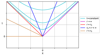
For the exterior solution, starting from , at we have straight lines that vary from with angle decreasing continuously and making when , till one reaches the line at ( ). If one is willing to include the interior solution in the same diagram, one could associate all the lines with angle again with the values of , similar to what occurs for [see comments below (18)]. Instead, we represent the interior solution by choosing a sign and interchanging the hyperbolic functions in (23) and (24), which makes that the lines at constant vary continuously from the red line in Fig. 1 till , corresponding to . We have omitted the horizontal hyperbolas at constant . Here, the exterior region is the upper part inside the ‘cone’, from to , and the interior region is delimited in the second quadrant by the lines and . The other two regions of a maximal extension, not shown, are merely a reflection.
Getting back to the distinct possibilities for , we have that and also admits hyperbolic sines and cosines as solutions. An appropriate selection is and . Now, (13) and the other relations are satisfied with , that is for positive. Although hyperbolic functions of are allowed, the simplest case is choosing the exponentials mentioned below Eq. (20), namely and -a positive sign was chosen. Inserting in and , we have,
| (28) |
and
| (29) |
respectively. As before, can be set equal to one without loss of generality, and for Schwarzschild solution it turns out to be useful , since then from (18) one obtains for the exterior solution, and where the defining surfaces now are hyperbolas at constant , with
| (30) |
That is, by choosing adequately the constant , we have obtained the usual Kruskal solution [2][3]. Moreover, from the perspective of the present work, (30) is the minimal solution that uniquely represents the interior and exterior solution to the event horizon [4]. The interior is included in the other transformations by selecting due to (18) as well as by interchanging the hyperbolic functions in (28) and (29). See Figure 2, where the maximal extension is shown, and lines at are omitted.
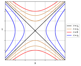
Recall the discussion from Section 3: negative can be describing interior or exterior solutions, and the correspondence is not one to one. However, both in this Kruskal-Szekeres case with hyperbolas at constant , as well as the Kruskal-type variation of Fig. 1 with lines in place of hyperbolas, we can select the signs in the integration constants, in such a way that exterior and interior solutions are uniquely represented in the same diagram.
As we shall see, the final case induces coordinates that don’t share this property, but will be interesting in other respects.
5. Pulsating coordinates.
Now we turn our attention for the final possibility dictated by the relations at the end of section 2. For in (15), we have that it allows to choose
| (31) |
where we have defined . We shall focus just in the case of having , , since would just interchange the role of the and coordinates and the sign of the conformal factor. Then, relation (12) in the form leads in this case to
| (32) |
where . This in turn implies that the constant in (13) is equal to , that is positive. One can readily see that in (14) we also have , and then we can select . Inserting this in (12) stated as , we have to integrate the relation
| (33) |
The result is
| (34) |
and consequently
| (35) |
Since we could have chosen the negative sign for , and is arbitrary, this gives us the possibility of choosing sines or cosines for and . For instance, by choosing and a sign in , previous relations yield the coordinate transformations and . By taking the differential and by substituting in (8), one can see that (17) is satisfied when . However, here goes to infinity whenever . Instead, we choose and negative sign in , which yields a similar selection:
| (36) |
and
| (37) |
Also, substitution in (17) yields the conformal factor
| (38) |
By comparing with the Kruskal-Szekeres or related coordinates such as those of Section 4, several differences arise. In place of having hyperbolas and lines at constant or , here in general one has ellipses or circumferences, since the curves at constant are given by
| (39) |
while at constant we have
| (40) |
Fig. (3) shows the mentioned behavior considering that the curves corresponds to constant (we chose for simplicity).
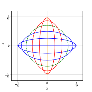
Here, one has that all the spacetime is compactified to maximum limits of in the coordinates and . Notice that the presence of any horizon makes to vary in an infinite range in any casual patch of the spacetime described by (2). This in turn implies that the surfaces corresponding to constant in pulsating coordinates make infinite oscillations between vertical and horizontal ellipses, passing through vertical lines, circumferences or horizontal lines for the special values , or , with a non-negative integer.
Clearly, this series of oscillations can be avoided for any finite domain of that does not include the event horizon. For instance, in the Schwarzschild case, take the decreasing values between the photon sphere () and the zero of the tortoise coordinate. By choosing , then we have first an horizontal ellipse with semimajor axis that converts into a circle when and then into vertical ellipses that asymptotically tend to a vertical line when .
Other case of interest include metrics that describe cosmological models. For instance, take the FLRW models
| (41) |
where is the cosmological time measured by an observer with comoving radial coordinate [10]. The subclass of FLRW solutions that can be converted to (2) are only those for which and where the only possible contribution to the energy momentum tensor is vacuum energy [7][11]. For the distinct possibilities allowed for the cosmological constant and the curvature parameter , this subclass of solutions includes de-Sitter or Anti-de-Sitter spaces, Lanczsos universe, Milne model or even Minkowski space [12][13]. Take for instance the de-Sitter solution, where and , with scale parameter . Here, the solution of (16) for the tortoise coordinate is , that induces again infinite oscillations in the variable (at constant), see Fig. 4.
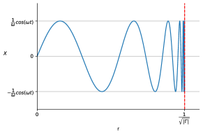
These oscillations become more dramatic as , the cosmological horizon. This in turn induces the mentioned oscillations between ellipses in the diagram.
Now consider Anti-de-Sitter space, where both and are negative. The scale parameter is obtained from the first Friedmann equation as [7]. Also, solving for the tortoise coordinate (16) we obtain , and then for this case goes from to when goes from to . By choosing , then (39) leads to a vertical line for that converts into vertical ellipses in in Fig. 3 (yellow lines), then into a circumference of radius and from there vertical ellipses for that approach the horizontal line as , which in Fig. 3 appear in blue lines.
Similar argument occurs to the surfaces at constant, where in agreement with (40) the change is from horizontal ellipses to vertical ones.
6. Final remarks.
In this work, we have studied an approach that relates several types of transformations for spherically symmetric spaces, that can be put in the form
| (42) |
This includes spaces associated describing black holes such as Schwarzschild, Reissner-Norström, but also allows for cosmological solutions such as de-Sitter, Anti-de-Sitter or Schwarzschild-de-Sitter, among others. Our approach relates several possible transformations to a flat conformal flat (1+1)-type when considering constant angles. The developments of Section 2, and in particular the sign of the product in Eq. (15), led us to derive three coordinate solutions: tortoise, Kruskal-Szekeres type and pulsating coordinates.
In Section 3 we obtained the tortoise case as the unique possibility for , and also mentioned some properties of the tortoise coordinates that where relevant for the other two general cases. Section 4 was devoted to analyze the case , where several combinations of exponential and hyperbolic functions appear. We mentioned two selections, one where lines denote spheres with constant , as well as the usual Kruskal-Szekeres transformation. Both elections allow a distinction of the interior and exterior regions in the same diagram.
As a final part, in Section 5 we introduced the notion of pulsating coordinates as an unexplored possibility for , which leads also to several possibilities for defining and in terms of trigonometric functions, from which we have selected an appropriate one, described by the relations (36)-(40). We argue that these solutions have the advantage of compactifying the space-time in a different way of the Penrose-Carter compactification. For instance, contrast the exponential grow implied by (28) and (29) in the the Kruskal diagram with the oscillatory behavior in the pulsating coordinates. This new system of coordinates present infinite oscillations between hyperbolas when taking into account all the domain of in a causally connected patch with an event horizon.
Throughout the article we have mentioned the Schwarzchild spacetime as the prototype for the analysis in all the coordinates presented. However, for the case of pulsating coordinates we have also contrasted what occurs in two cosmological models of interest, namely de-Sitter (dS) and Anti-de-Sitter (AdS). We find that the behavior is better for the AdS solution, since in this case one can obtain a unique transition from vertical to horizontal ellipses. Given the fact that the crossing of ellipses with the -axis is unique for any value of going from when to when (), we have a natural dimensional reduction for the AdS spacetime that emulates the Poincaré mapping, useful in the study of dynamical systems [14]. This line of thinking, as well as the possibility of relating exterior and interior solutions in black holes and cosmology [15], or the specific use for other relevant metrics (see [16]-[18] and References therein), are left as possible future works.
Acknowledgments: ASR and BMO acknowledge a graduate fellowship grant by CONACYT-Mexico.
Appendix. Existence of conformal flat transformation in (1+1) dimensions.
Any (1+1) metric can be put in a conformal flat way , where . The plainer way to see it is to consider null coordinates and . Here , where is the basis for any null vector in the v-direction. Since the dual version in terms of the inverse metric is , and given the one-form , this is the same as , that can be seen as the definition of a null coordinate, and analog definitions for the other null coordinate [19]. Defining and , those relations can be casted as the transformation of the metric to new coordinates, in the form
| (A.1) |
and
| (A.2) |
Now, if has diagonal elements equal to zero, so does , since in this case and for the inverse to exist. It follows that and similar argument yields . Then, in terms of null coordinates the system simplifies to
| (A.3) |
Rotating coordinates by means of and , the metric takes the assumed conformal form
| (A.4) |
where .
References
- [1] T. Dray, Differential forms and the geometry of general relativity (CRC Press, Boca Raton FL, 2014) pp. 34-55, https://doi.org/10.1201/b17620.
- [2] M. D. Kruskal, Maximal Extension of Schwarzschild Metric, Phys. Rev. 119 (1960) 1743, https://doi.org/10.1103/PhysRev.119.1743.
- [3] G. Szekeres, On the Singularities of a Riemannian Manifold, Publ. Math. Debrecen 7 (1960) 285, https://doi.org/10.1023/A:1020744914721.
- [4] C. W. Misner, K.S. Thorne, and J.A. Wheeler. Gravitation (W. H. Freeman and Company, San Francisco CA, 2004) pp. 820-835.
- [5] S. M. Carroll, Spacetime and geometry: An introduction to general relativity (Addison-Wesley, San Francisco CA, 2004) pp. 329-336.
- [6] T. Jacobson, When is ?, Class. Quant. Grav. 24 (2007) 5717, https://doi.org/10.1088/0264-9381/24/22/N02.
- [7] J. A. Nieto, E. A. León, and C. García-Quintero, ”Cosmological-static metric correspondence and Kruskal type solutions from symmetry transformations”, Rev. Mex. Fís., vol. 68, no. 4 Jul-Aug, pp. 040701 1-, Jun. 2022, https://doi.org/10.31349/RevMexFis.68.040701.
- [8] K. Schwarzschild, ”On the Gravitational Field of a Mass Point According to Einstein’s Theory,” Abh. Konigl. Preuss. Akad. Wissenschaften Jahre 1906,92, Berlin, 1907, vol. 1916. pp. 189-196, Jan. 1916.
- [9] K. A. Bronnikov, E. Elizalde, S. D. Odintsov, and O. B. Zaslavskii, Horizon versus singularities in spherically symmetry space-times, Phys. Rev. D 78 (2008) 060449, https://doi.org/10.1103/PhysRevD.78.064049.
- [10] P. J. E. Peebles. Principles of physical cosmology (Princeton University Press, Princeton NJ, 1993) pp. 70-78.
- [11] Florides, P.S. The Robertson-Walker metrics expressible in static form. Gen. Rel. Grav. 12 (1980) 563, https://doi.org/10.1007/BF00756530.
- [12] F. Melia, Cosmological redshift in Friedmann-Robertson-Walker metrics with constant space-time curvature, MNRAS 422 (2012) 1418, https://doi.org/10.1111/j.1365-2966.2012.20714.x.
- [13] A. Mitra, When can an ”Expanding Universe” look ”Static” and vice versa: A comprehensive study, Int. J. Mod. Phys D 24 (2015), https://doi.org/10.1142/S0218271815500327.
- [14] M. W. Hirsch, S. Smale, R. L. Devaney, Differential equations, dynamical systems, and an introduction to chaos (Academic Press, Waltham MA, 2013) pp. 11-15, https://doi.org/10.1016/C2009-0-61160-0.
- [15] C. Aviles-Niebla, P. A. Nieto-Marin, and J. A. Nieto, Towards exterior/interior correspondence of black holes, Int. J. Geom. Meth. Mod. Phys. 17 (2020) 2050180, https://doi.org/10.1142/S0219887820501807.
- [16] J. C. Graves, and D. R. Brill, Oscillatory Character of Reissner-Nordström Metric for an Ideal Charged Wormhole, Phys. Rev. 120 (1960) 1507, https://doi.org/10.1103/PhysRev.120.1507.
- [17] J. P. S. Lemos, D. L. F. G. Silva, Maximal extension of the Schwarzschild metric: From Painlevé-Gullstrand to Kruskal-Szekeres, Annals of Physics. 430 (2021) 168497, https://doi.org/10.48550/arXiv.2005.14211.
- [18] A. V. Toporensky, O. B. Zaslavskii, Regular Frames for Spherically Symmetric Black Holes Revisited, Symmetry 14 (2022) 40, https://doi.org/10.3390/sym14010040.
- [19] R. D’Inverno, Introducing Einstein’s relativity (Oxford University Press, Oxford UK, 1992) pp. 85-90.