The strong-coupling quantum thermodynamics of quantum Brownian motion
based on the exact solution of its reduced density matrix

Abstract

We derive the quantum thermodynamics of quantum Brownian motion from the exact solution of its reduced density matrix. By exactly traced over all the reservoir states, we solve analytically and exactly the reduced density matrix of the Brownian particle from the total equilibrium thermal state of the system strongly entangling with its reservoir. We find that the reduced Hamiltonian and the reduced partition function of the Brownian particle must be renormalized significantly, as be generally shown in the nonperturbative renormalization theory of quantum thermodynamics we developed recently. A momentum-dependent potential is generated naturally from the linear coupling between the Brownian particle and the reservoir particles, after all the reservoir states are completely traced out. Moreover, beyond the weak coupling limit, it is imperative to take into account the non-negligible changes of the reservoir state induced by the system-reservoir coupling, in order to obtain the correctly reduced partition function of the Brownian particle. Using the exact solutions of the reduced density matrix, the renormalized Hamiltonian and the reduced partition function for the Brownian particle, we show that the controversial results from the different definitions of internal energy and the issue of the negative heat capacity in the previous studies of strong-coupling quantum thermodynamics are resolved.

I Introduction

The study of quantum thermodynamics beyond the weak-coupling limit has received tremendous attentions in recent years. This is because under the strong coupling between the system and its reservoir, many new thermodynamic phenomena may occurs and the foundation of thermodynamic laws may also be challenged. For example, it has been realized recently that quantum features such as quantum coherence and quantum entanglement could be exploited to enhance the energy conversion efficiency of nanoscale systems engine1 ; engine2 ; engine3 ; engine4 ; engine5 ; engine6 ; engine7 ; WM2 , which has significant implications for designing and optimizing quantum heat engines in the future. More importantly, quantum thermodynamics under strong coupling involves reinterpretation and new understanding of thermodynamic laws. The traditional thermodynamic laws may require modifications or extensions to accommodate the quantum features in the nano- and atomic scale systems WM1 ; WM3 ; QT1 ; QT2 ; QT3 ; QT4 ; QT5 ; QT6 ; Seifert16 ; Jarzynski17 ; seclaw1 ; seclaw2 ; seclaw3 ; heat ; PH07 ; CB2022 ; entangle1 ; entangle2 ; entangle3 ; PH06 ; PH08 ; PH09 ; nega4 ; nega5 ; HC2 ; PH20 ; MF1 ; MF2 ; MF3 ; MF4 ; MF5 ; MF6 . This motivates researchers to attempt to explore and establish a general framework for quantum thermodynamics at strong coupling between the system and its reservoir, to describe quantum thermodynamic behaviors and to better understand the foundation of thermodynamics Seifert16 ; Jarzynski17 ; WM1 . The investigation of quantum heat capacity at strong coupling also becomes an important issue because it may be inherently associated with quantum entanglement entangle1 ; entangle2 ; entangle3 and it pertains to the issues of the validity of the third law of thermodynamics PH06 ; PH08 ; PH09 ; nega4 ; nega5 ; HC2 .

However, due to the strong coupling in the quantum regime, many thermodynamic quantities, including the internal energy and the heat capacity, have to be redefined. Some contradictory results of heat capacity in strong-coupling quantum Brownian motion were found and discussed PH06 ; PH08 ; PH09 , which arisen from the inconsistency of the internal energy under different definitions. In order to overcome the difficulties of including the new effect arisen from strong coupling, an effective Hamiltonian known as the Hamiltonian of mean force is widely used PH20 ; MF1 ; MF2 ; MF3 ; MF4 ; MF5 ; MF6 ; Seifert16 ; Jarzynski17 , in which the thermal state of the reservoir is supposed to be invariant because of its macroscopic nature. Nevertheless, as shown in our recent work WM1 , for any system coupling to a thermal reservoir, with the strong system-reservoir coupling, both the system and the reservoir undergo a non-equilibrium dynamical evolution, and the final equilibrium temperature of the system-reservoir state must be renormalized. This indicates that the strong coupling between the system and reservoirs will result in a non-negligible change for both the system and the reservoir states, which naturally questions the validity of the Hamiltonian of mean force in the strong coupling regime.

On the other hand, we also find that the system Hamiltonian must be renormalized in the way that the strong coupling effect between the system and the reservoir must be correctly incorporated after tracing over all the reservoir states. In our recent work YW2022 , we have derived the exact master equation of a generalized quantum Brownian motion analytically, which goes beyond the previous derivations of the master equation for the quantum Brown motion by Caldeira and Leggett for a Ohmic spectral density Leggett1983 and by Hu, Paz and Zhang for color noise HPZ1992 . In this recent work YW2022 , all the physical quantities have been renormalized in the standard framework of many-body nonequilibrium dynamics. It shows that the renormalization not only modifies the system Hamiltonian, but also induces a momentum-dependent potential to the Brownian particle. In other words, after tracing over all the reservoir states, the renormalized quantum Brownian particle contains a system-reservoir coupling induced new potential that was not recognized in the previous studies Leggett1983 ; HPZ1992 , and are also omitted further in the recent investigations to strong-coupling quantum thermodynamics PH20 ; HC2 ; Grabert1 ; MF2 ; MF3 ; MF4 ; MF5 ; MF6 , even in cases where some of them did not employ the approach of the Hamiltonian of mean force.

Furthermore, in other previous studies QBMME1 ; QBMME2 , including our recent work YW2022 , it was pointed out that renormalization effects stemming from the system-reservoir coupling can result in the phenomenon of the Brownian particle becoming squeezed. The effects of particle squeezing in quantum thermodynamics remain an evolving field of study to date. Recent research has unveiled novel thermodynamic behaviors exhibited by systems involving particle squeezing effects squeezed thermal1 ; squeezed thermal2 ; squeezed thermal3 ; squeezed thermal4 ; squeezed thermal5 ; squeezed thermal6 , where the influence of squeezing parameters on thermodynamic quantities such as thermal population, internal energy, and work has also been proposed. Nevertheless, in previous studies on the quantum thermodynamics of quantum Brownian motion PH06 ; PH08 ; PH09 ; PH20 ; nega4 ; nega5 ; HC2 ; Grabert1 ; MF1 ; MF2 ; MF3 ; MF4 ; MF5 ; MF6 , there was a lack of manifesting the influence of the renormalization-induced squeezing effects of Brownian particle towards thermodynamic quantities. In fact, we find that if the system Hamiltonian is correctly renormalized YW2022 , the resulting Brownian particle, when it reaches the thermal equilibrium with its bath, is characterized by a squeezed thermal state. A detailed discussion of this matter will be presented in the next section, where we will also show the relation between the momentum-dependent potential and the renormalization-induced squeezing of the Brownian particle.

After all, in this paper, we study analytically the quantum Brownian particle interacting weak or strongly with its reservoir, where both the Brownian particle and all the particles in the reservoir are modeled as harmonic oscillators that are linearly coupled to each other Feynman1963 ; Leggett1983 . We begin with a total thermal equilibrium state in which the Brownian particle and the reservoir particles are entangled completely, which can be easily realized under the quantum dynamical evolution for an arbitrary state of the Brownian particle coupling to a thermal reservoir WM1 . The total thermal equilibrium state is usually called a partition-free state in the literature, which is indeed a Gibbs state of the total system (Brownian particle plus its reservoir). We then use the coherent-state integral approach and group theory to trace over explicitly all the reservoir states without using any assumption or approximation. From this analytical solution, we find how the state of Brownian particles is intricately influenced by the reservoir, and how a momentum-dependent potential (a squeezed pairing effect) is naturally generated to the Brownian motion from the linear coupling of the Brownian particle and the reservoir. Furthermore, we utilize the faithful matrix representation in group theory Gilmore ; group ; bookw to deal with the operator ordering problem and obtain exactly the renormalized Hamiltonian, the corresponding reduced density matrix, and the renormalized partition function of the Brownian particle. Such a rigorous derivation has not been carried out in the literature, due to its difficulty without the help of group theory methodology group . It shows that the reduced density matrix of the Brownian particle can be also expressed as a Gibbs state with the renormalized Hamiltonian which contains inevitably a momentum-dependent potential that is generated from the system-reservoir coupling, which has not been noticed in the previous studies PH06 ; PH08 ; PH20 ; HC2 ; Grabert1 ; MF1 ; MF2 ; MF3 ; MF4 ; MF5 ; MF6 .

By further diagonalizing the renormalized Hamiltonian through a Bogoliubov transformation, we show that the Bogoliubov quasiparticle is subjected to a harmonic oscillator potential in a new coordinate system. As an result, we obtain an extended Bose-Einstein distribution for Brownian particle with pairing interactions, which describes the relation between particle occupation and squeezing parameter as well as the renormalized frequency and pairing strength. As a self-consistent check, we study the heat capacity based respectively on the Hamiltonian and the partition function of the renormalized Brownian particle. In order to compare our results with the debated results in the literature, we also numerically calculate the heat capacity based on the incomplete-renormalized Hamiltonian and incomplete-renormalized partition function of the Brownian particle that used in Refs. PH06 ; PH08 ; PH09 ; nega4 ; nega5 and show how contradictory results were generated from the improper definitions of internal energy and partition function.

The rest of the paper is organized as follows. In Sec. II, we solve the reduced density matrix and the corresponding renormalized system Hamiltonian based on our nonperturbation renormalization theory for quantum thermodynamics WM1 . The analytical analysis and numerical results of thermodynamic quantities are presented in Sec. III. A conclusion is given in Sec. IV. The detailed derivations of the formulas are presented in Appendix.

II The exact reduced density matrix of Brownian particle

The quantum Brownian motion describes the behavior of a quantum particle interacting with a thermal bath. It is modeled by the Hamiltonian Feynman1963 ; Leggett1983 ,

$$H_{\rm tot}= H_{\textsc{S}}+H_{\textsc{E}}+H_{\textsc{SE}}$$

$$= \dfrac{P^{2}}{2m}+\dfrac{1}{2}M\Omega^{2}Q^{2}+\sum\limits_{k}\dfrac{f_{k}^{2}Q^{2}}{2m_{k}\omega_{k}^{2}}$$

$$+\sum\limits_{k}\left(\dfrac{p_{k}^{2}}{2m_{k}}+\dfrac{1}{2}m_{k}\omega_{k}^{2}x_{k}^{2}\right)-\sum\limits_{k}f_{k}Qx_{k},$$ (1)

in which the Brownian particle $(P,Q)$ is considered to be trapped in a harmonic potential, and the last term in $H_{\textsc{S}}$ represents the counter-term to remove the possible unphysical divergence of the renormalized frequency-shift. The reservoir is modeled as a collection of an infinite number of harmonic oscillators $(p_{k},x_{k})$ with a continuous frequency distribution. The system-reservoir interaction is described by linear couplings between the system particle and all the particles in the reservoir, depicted by the last term in the above Hamiltonian.

For the convenient calculations in the coherent state basis group ; bookw , we rewrite the above Hamiltonian in the particle number representation,

$$H_{\rm tot}= \hbar\omega_{\textsc{S}}a^{\dagger}a+\sum\limits_{k}\hbar\omega_{k}b_{k}^{\dagger}b_{k}$$

$$+\sum\limits_{k}\hbar V_{k}\left(a^{\dagger}b_{k}+b_{k}^{\dagger}a+a^{\dagger}b_{k}^{\dagger}+b_{k}a\right),$$ (2)

where $a^{\dagger}$ and $b_{k}^{\dagger}$ ($a$ and $b_{k}$) are the bosonic creation (annihilation) operators for the system and the reservoir with energy quanta $\hbar\omega_{\textsc{S}}$ and $\hbar\omega_{k}$, respectively. The effective frequency of the system incorporating the counter-term is given by $\omega_{\textsc{S}}^{2}=\Omega^{2}+\sum_{k}f_{k}^{2}/Mm_{k}\omega_{k}^{2}$. The coupling parameter $V_{k}=-f_{k}/2\sqrt{Mm_{k}\omega_{S}\omega_{k}}$ is the coupling amplitude between the system and the k-mode in the reservoir, which can be weak or strong. The form of Eq. (II), which is exactly the same as Eq. (1), shows that the linear coupling between the system and the reservoir contains the particle pair production and annihilation, which will modify significantly the renormalized system Hamiltonian when the coupling becomes strong, as we will see later.

To study the thermodynamics of quantum Brownian motion, we consider the total system to be in a thermal equilibrium state. Such a state can always be realized when the system and the reservoir reach their steady state, even if they begin with a decoupled initial state, i.e., the system can be in an arbitrary initial state and the reservoir is initially in a thermal reservoir WM1 . Then the final density matrix of the total equilibrium state is given by

$$\rho_{\rm tot}=\frac{1}{Z_{\rm tot}}e^{-\beta H_{\rm tot}},$$ (3)

where $\beta=1/k_{\textsc{B}}T$, and $T$ is the equilibrium temperature of the total system at the steady state. Equation (3) is a highly entangled state between the system and its reservoir.

The key issue to derive the quantum thermodynamics of a Brownian particle lies on the state of the Brownian particle itself, which is completely described by the reduced density matrix $\rho_{S}$. The reduced density matrix $\rho_{S}$ is determined by the partial trace over all the reservoir states from the total density matrix $\rho_{\rm tot}$,

$$\rho_{\textsc{S}}=\operatorname{Tr}_{\textsc{E}}[\rho_{\rm tot}]=\frac{1}{Z_{\rm tot}}\operatorname{Tr}_{\textsc{E}}[e^{-\beta H_{\rm tot}}],$$ (4)

which is usually a very difficult task. Fortunately, for the quantum Brownian motion, the total density matrix is a Gaussian-type state so that the partial trace is exactly doable with the help of group theory and coherent state method group . Explicitly, in the coherent state representation, the total density matrix can be expressed as

$$\langle\bm{z}|\rho_{\rm tot}|\bm{z^{\prime}}\rangle\!=\!\dfrac{\sqrt{\det\bm{\Omega}}}{Z_{\rm tot}}\exp\!\left[\dfrac{1}{2}\begin{pmatrix}\bm{z^{\dagger}}&\bm{z^{\prime T}}\end{pmatrix}\!\!\begin{pmatrix}\bm{\Omega}&\bm{\Pi}\\ \bm{\Pi^{*}}&\bm{\Omega^{*}}\end{pmatrix}\!\!\begin{pmatrix}\bm{z^{\prime}}\\ \bm{z^{*}}\end{pmatrix}\!\right],$$ (5)

where $|\bm{z}\rangle=|z_{S},\bm{z_{E}}\rangle=\exp\{z_{S}a^{\dagger}+\sum_{k}z_{k}b^{\dagger}_{k}\}|0\rangle$ is the unnormalized coherent state which is also the eigenstate of the annihilation operators $(a,\{b_{k}\})$ with complex eigenvalue $\bm{z}=(z_{S},\bm{z}_{E})$. The normalized factor of the coherent states has been moved into the integral measure of the coherent state identity resolution for the convenience of calculations, as one will see later. The factor $\sqrt{\det\bm{\Omega}}$ comes from the normal ordering of the operators in coherent state representation norder1 ; norder2 , that is, $\langle z|A(a^{\dagger},a)|z^{\prime}\rangle=\vcentcolon\mathrel{A(z^{*},z^{\prime})}\vcentcolon$. More explicitly, the constant arises from the relation $\langle z|e^{\kappa(a^{\dagger}a+aa^{\dagger})}|z^{\prime}\rangle=e^{\kappa}\exp[{e^{\kappa}(z^{*}z^{\prime}+z^{\prime}z^{*})}]$, see more detail in Eq. (53). The matrix block $\bm{\Omega}$ is a Hermitian matrix and $\bm{\Pi}$ is an symmetric matrix, both are $(k_{c}+1)\times(k_{c}+1)$ matrices,

$$\bm{\Pi}=\begin{pmatrix}\Pi_{SS}&\bm{\Pi}_{S\bm{E}}\\ \bm{\Pi}_{S\bm{E}}^{*}&\bm{\Pi_{EE}}\end{pmatrix},\ \bm{\Omega}=\begin{pmatrix}\Omega_{SS}&\bm{\Omega}_{S\bm{E}}\\ \bm{\Omega}_{S\bm{E}}^{*}&\bm{\Omega_{EE}}\end{pmatrix}$$ (6)

where $k_{c}$ is the total number of the oscillation modes in the reservoir and is infinite in principle. With the aid of the faithful matrix representation of a subgroup of the Lie group $Sp(2k_{c}+4)$ group (see appendix A for the detail derivation), they are given by

$$\bm{\widetilde{\Omega}} =\bigg{\{}\!\begin{pmatrix}\bm{0}&\bm{I}\end{pmatrix}\exp\bigg{[}\begin{pmatrix}\bm{D}&\bm{R},\\ -\bm{\hat{R}}&-\bm{\widetilde{D}}\end{pmatrix}\bigg{]}\begin{pmatrix}\bm{0}\\ \bm{I}\end{pmatrix}\!\bigg{\}}^{-1}$$ (7a)

$$\bm{\Pi} =\bigg{\{}\!\begin{pmatrix}\bm{I}&\bm{0}\end{pmatrix}\exp\bigg{[}\begin{pmatrix}\bm{D}&\bm{R}\\ -\bm{\hat{R}}&-\bm{\widetilde{D}}\end{pmatrix}\bigg{]}\begin{pmatrix}\bm{0}\\ \bm{I}\end{pmatrix}\!\bigg{\}}\bm{\widetilde{\Omega}},$$ (7b)

where $\widetilde{\bm{D}}$ denotes a reflection in the minor diagonal of $\bm{D}$, and $\hat{\bm{R}}$ is a reflection in the major diagonal of the $\bm{R}$. The matrices $\bm{D}$ and $\bm{R}$ are determined by the parameters in the total Hamiltonian $H_{\rm tot}$ of Eq. (II),

$$\bm{D}=-\dfrac{\hbar\beta}{2}\begin{pmatrix}\omega_{S}&\bm{V}_{S\bm{E}}\\ \bm{V}_{S\bm{E}}^{\dagger}&\bm{\omega_{E}}\end{pmatrix},\ \bm{R}=-\dfrac{\hbar\beta}{2}\begin{pmatrix}\bm{\bar{V}}_{S\bm{E}}&0\\ \bm{0}&\bm{V}_{S\bm{E}}^{\dagger}\end{pmatrix},$$ (8)

in which $\bm{\bar{V}}_{S\bm{E}}$ is the inversion of $\bm{V}_{S\bm{E}}$. More explicitly,

$$\bm{\omega_{E}}=\!\begin{pmatrix}&\omega_{k_{1}}&&&\\[-5.69054pt] &&\omega_{k_{2}}&&\mbox{\Huge 0}\\ &\mbox{\Huge 0}&&&\ddots\end{pmatrix}\!,\ \bm{V}_{S\bm{E}}=\begin{pmatrix}V_{k_{1}}&V_{k_{2}}&\cdots\end{pmatrix},$$ (9a)

$$\bm{\widetilde{\omega}_{E}}=\!\begin{pmatrix}&\ddots&&&\mbox{\Huge 0}\\ &&&\omega_{k_{2}}&\\[-5.69054pt] &\mbox{\Huge 0}&&&\omega_{k_{1}}\end{pmatrix}\!,\ \bm{\bar{V}}_{S\bm{E}}=\begin{pmatrix}\cdots&V_{k_{2}}&V_{k_{1}}\end{pmatrix}.$$ (9b)

Taking the trace over all the reservoir states via the Gaussian integral (See AppendixA), the reduced density matrix of the Brownian particle in the coherent state representation can be obtained analytically,

$$\langle z_{S}|{\rho_{S}} |z^{\prime}_{S}\rangle=\int\!d\mu(\bm{z_{E}})\langle z_{S},\bm{z_{E}}|\rho_{tot}|z_{S}^{\prime},\bm{z_{E}}\rangle$$

$$= \dfrac{1}{Z^{r}_{S_{0}}}\exp\left[\dfrac{1}{2}\begin{pmatrix}z_{S}^{\dagger}&z_{S}^{\prime T}\end{pmatrix}\!\begin{pmatrix}\Omega_{S}&\Pi_{S}\\ \Pi_{S}^{*}&\Omega_{S}\end{pmatrix}\!\begin{pmatrix}z_{S}^{\prime}\\ z_{S}^{*}\end{pmatrix}\right]$$ (10)

Here the coherent state integral measure $d\mu(\bm{z_{E}})=\prod_{k}\frac{dz_{k}dz^{*}_{k}}{2\pi i}e^{-|z_{k}|^{2}}$ and the factor $e^{-|z_{k}|^{2}}$ comes from the normalization of the coherent state. The resulting matrix after the integral is found to be

$$\begin{pmatrix}\Omega_{S}&\Pi_{S}\\ \Pi_{S}^{*}&\Omega_{S}\end{pmatrix} =\begin{pmatrix}\Omega_{SS}&\Pi_{SS}\\ \Pi_{SS}^{*}&\Omega_{SS}\end{pmatrix}+\!\begin{pmatrix}\bm{\Omega}_{S\bm{E}}&\bm{\Pi}_{S\bm{E}}\\ \bm{\Pi}^{*}_{S\bm{E}}&\bm{\Omega}^{*}_{S\bm{E}}\end{pmatrix}\!$$

$$\times\left[\bm{I}\!-\!\begin{pmatrix}\bm{\Omega_{EE}}&\bm{\Pi_{EE}}\\ \bm{\Pi_{EE}^{*}}&\bm{\Omega^{*}_{EE}}\end{pmatrix}\!\right]^{-1}\!\!\begin{pmatrix}\bm{\Omega}_{\bm{E}S}&\bm{\Pi}_{\bm{E}S}\\ \bm{\Pi}^{*}_{\bm{E}S}&\bm{\Omega}^{*}_{\bm{E}S}\end{pmatrix}\!,$$ (11)

and the coherent-state partition function of the renormalized Brownian particle is given by

$$Z^{r}_{S_{0}}= \dfrac{Z_{\rm tot}}{\sqrt{\det\bm{\Omega}}}\left\|\bm{1}-\begin{pmatrix}\bm{\Omega_{EE}}&\bm{\Pi_{EE}}\\ \bm{\Pi^{*}_{EE}}&\bm{\Omega^{*}_{EE}}\end{pmatrix}\right\|^{1/2}$$

$$= \sqrt{\dfrac{1}{(1-\Omega_{S})^{2}-|\Pi_{S}|^{2}}}.$$ (12)

In general, the thermal reservoir is significantly larger compared to the system it interact with, which means that the number of its oscillation modes $k_{c}$ is infinite, and so do the dimension of $\bm{\Omega}$ and $\bm{\Pi}$. In this situation, it is very difficult to directly obtain the renormalization of the system encompassing all the reservoir effect through the matrix operations in Eq. (11). Therefore, we also apply the imaginary-time path integral approach in the coherent state representation (See Appendix B) to calculate the partial trace over the reservoir’s states that is characterized by a continuous spectral density $J(\epsilon)=2\pi\sum_{k}|V_{k}|^{2}\delta(\epsilon-\epsilon_{k})$. After integrating out all the degree of freedom of the reservoir, we have

$$\dfrac{d}{d\tau}\left.\begin{pmatrix}\Omega_{S}(\tau)&\Pi_{S}(\tau)\\ \Pi_{S}^{*}(\tau)&\Omega_{S}^{*}(\tau)\end{pmatrix}\right|_{\tau\rightarrow\hbar\beta}\!\!\!\!=\!\begin{pmatrix}\!-\epsilon_{S}&0\\ 0&\epsilon_{S}\!\end{pmatrix}\begin{pmatrix}\Omega_{S}(\tau)&\Pi_{S}(\tau)\\ \Pi_{S}^{*}(\tau)&\Omega_{S}^{*}(\tau)\end{pmatrix}$$

$$+\!\int_{0}^{\hbar\beta}\!\!d\tau^{\prime}\bigg{\{}\!\begin{pmatrix}g(\hbar\beta-\tau^{\prime})&g(\hbar\beta-\tau^{\prime})\\ g(\tau^{\prime}-\hbar\beta)&g(\tau^{\prime}-\hbar\beta)\end{pmatrix}\!\begin{pmatrix}\Omega_{S}(\tau^{\prime})&\Pi_{S}(\tau^{\prime})\\ \Pi_{S}^{*}(\tau^{\prime})&\Omega_{S}^{*}(\tau^{\prime})\end{pmatrix}$$

$$+\![g^{\prime}(\tau^{\prime}\!-\!\hbar\beta)\!+\!g^{\prime}(\hbar\beta\!-\!\tau^{\prime})]\!\begin{pmatrix}1&\!1\\ -\!1&\!-\!1\end{pmatrix}\!\begin{pmatrix}\Omega_{S}(\tau^{\prime})&\Pi_{S}(\tau^{\prime})\\ \Pi_{S}^{*}(\tau^{\prime})&\Omega_{S}^{*}(\tau^{\prime})\end{pmatrix}\!\!\bigg{\}}$$ (13)

subjected to the initial conditions $\Omega_{S}(0)=1$ and $\Pi_{S}(0)=0$, where the integral kernels $g(\tau)$ and $g^{\prime}(\tau)$ are determined by the spectral density $J(\omega)=2\pi\sum_{k}|V_{k}|^{2}\delta(\omega-\omega_{k})$

$$g(\tau) =\int\dfrac{d\omega}{2\pi}J(\omega)e^{-\omega\tau},$$ (14a)

$$g^{\prime}(\tau) =\int\dfrac{d\omega}{2\pi}J(\omega)e^{-\omega\tau}/(e^{\beta\hbar\omega}-1).$$ (14b)

Note that the integro-differential equation Eq. (13) is solvable only for $\tau\rightarrow\hbar\beta$ so that the periodic boundary condition along the imaginary time $\tau$ can be satisfied (See Appendix B for details). Thus, the solutions of $\Omega_{S}(\tau)$ and $\Pi_{S}(\tau)$ at the given temperature $\tau=\beta$ are given by the following inverse Laplace transformation

$$\begin{pmatrix}\Omega_{S}(\hbar\beta)&\Pi_{S}(\hbar\beta)\\ \Pi_{S}^{*}(\hbar\beta)&\Omega_{S}^{*}(\hbar\beta)\end{pmatrix}=\mathcal{L}^{-1}\left[\begin{pmatrix}s+\omega_{S}+\Sigma(s)+\Sigma^{\prime}(s)+\Sigma^{\prime}(-s)&\Sigma(s)+\Sigma^{\prime}(s)+\Sigma^{\prime}(-s)\\ \Sigma(-s)-\Sigma^{\prime}(s)-\Sigma^{\prime}(-s)&s-\omega_{S}+\Sigma(-s)-\Sigma^{\prime}(s)-\Sigma^{\prime}(-s)\end{pmatrix}^{-1}\right],$$ (15)

where $\Sigma(s)=\mathcal{L}[g(\tau)]$ and $\Sigma^{\prime}(s)=\mathcal{L}[g^{\prime}(\tau)]$ are the Laplace transform of the integral kernels.

Now, using the same technique of Gaussian integrals, we can find explicitly the particle occupation $n=\operatorname{Tr}[a^{\dagger}a\rho_{S}]$ and the squeezing parameter $s=\operatorname{Tr}[aa\rho_{S}]$ in terms of the matrix element $\Omega_{S}$ and $\Pi_{S}$,

$$n=\dfrac{\Omega_{S}(1-\Omega_{S})+|\Pi_{S}|^{2}}{(1-\Omega_{S})^{2}-|\Pi_{S}|^{2}},$$ (16a)

$$s=\dfrac{\Pi_{S}}{(1-\Omega_{S})^{2}-|\Pi_{S}|^{2}}.$$ (16b)

Alternatively, the matrix elements $\Omega_{S}$ and $\Pi_{S}$ in Eq. (II) can be expressed in terms of the physically observable correlation functions, namely the occupation $n$ and the squeezing $s$,

$$\Omega_{S}=1-\dfrac{1+n}{(1+n)^{2}-|s|^{2}},$$ (17a)

$$\Pi_{S}=\dfrac{s}{(1+n)^{2}-|s|^{2}}.$$ (17b)

Furthermore, by applying the faithful matrix representation of $H_{6}$, a subgroup of $Sp(4)$ group , the reduced density matrix $\rho_{S}$ of Eq. (II) can be solved explicitly (see Appendix A),

$$\rho_{S}\!=\!\dfrac{1}{Z^{r}_{S}}\exp\left[\eta(a^{\dagger}a+aa^{\dagger})+\delta a^{\dagger 2}+\delta^{*}a^{2}\right],$$ (18)

where the renormalized partition function $Z_{S}^{r}$ and the factors $\eta$ and $\delta$ of the reduced density matrix $\rho_{S}$ in Eq. (18) can be expressed in terms of the particle occupation $n$ and the squeezing parameter $s$ as following:

$$\eta=\dfrac{n+\frac{1}{2}}{2\sqrt{\left|(n+\frac{1}{2})^{2}-|s|^{2}\right|}}\ln\left[\dfrac{\sqrt{\left|(n+\frac{1}{2})^{2}-|s|^{2}\right|}-\frac{1}{2}}{\sqrt{\left|(n+\frac{1}{2})^{2}-|s|^{2}\right|}+\frac{1}{2}}\right]$$ (19a)

$$\delta=\dfrac{-s}{2\sqrt{\left|(n+\frac{1}{2})^{2}-|s|^{2}\right|}}\ln\left[\dfrac{\sqrt{\left|(n+\frac{1}{2})^{2}-|s|^{2}\right|}-\frac{1}{2}}{\sqrt{\left|(n+\frac{1}{2})^{2}-|s|^{2}\right|}+\frac{1}{2}}\right]$$ (19b)

$$Z^{r}_{S}=\sqrt{n^{2}+n-|s|^{2}}.$$ (19c)

Thus, the reduced density matrix of the Brownian particle is completely solved from the total thermal equilibrium state of the system coupled to the reservoir, from which quantum thermodynamics of the Brownian particle can be unambiguously studied.

In particular, the renormalized partition function of the Brownian particle in Eq. (18) is also given $Z^{r}_{S}=\sqrt{\Omega_{S}}Z^{r}_{S_{0}}$ (see Appendix A). Substituting Eq. (12) into Eq. (19c), we find the relation between the renormalized partition function $Z^{r}_{S}$ and the total partition function $Z_{\rm tot}$ as following:

$$Z^{r}_{S} =\sqrt{\dfrac{\Omega_{S}}{(1-\Omega_{S})^{2}-|\Pi_{S}|^{2}}}$$

$$=Z_{\rm tot}\sqrt{\dfrac{\Omega_{S}}{\det\bm{\Omega}}}\left\|\bm{1}-\begin{pmatrix}\bm{\Omega_{EE}}&\bm{\Pi_{EE}}\\ \bm{\Pi^{*}_{EE}}&\bm{\Omega^{*}_{EE}}\end{pmatrix}\right\|^{1/2}.$$ (20)

As shown in Eq. (7), Eq. (8) and Eq. (11), the matrix element $\bm{\Omega}$ as well as $\bm{\Omega_{EE}}$ and $\bm{\Pi_{EE}}$ are not only related to the reservoir mode frequencies $\bm{\omega_{E}}$, but also depend on the system frequency $\omega_{S}$ and the system-reservoir coupling $\bm{V}_{S\bm{E}}$. In other words, Eq. (II) implies the fact that the state of reservoir cannot remain unchanged. Instead, the reservoir state must also have the corresponding changes induced by the system-reservoir coupling, in particular when the coupling becomes strong. As a consequence,

$$Z^{r}_{S}\neq \frac{Z_{\rm tot}}{Z_{E}},\leavevmode\nobreak\ \leavevmode\nobreak\ {\rm where}\leavevmode\nobreak\ \leavevmode\nobreak\ Z_{E}\equiv\operatorname{Tr}_{E}[\exp(-\beta H_{E})],$$ (21)

namely, the partition function of the Brownian particle cannot be naively expressed as the partition function of the total system divided by the partition function $Z_{E}$ of the reservoir alone. This is very different from the conventionally assumption made in many previous works PH06 ; PH08 ; PH09 ; PH20 ; nega4 ; nega5 ; HC2 ; Grabert1 ; MF1 ; MF2 ; MF3 ; MF4 ; MF5 ; MF6 ; Seifert16 ; Jarzynski17 where one believes that the reservoir is large enough so that its state changes can be ignored. However, as we will show in the next section, it is this commonly accepted assumption that generates the inconsistent results in the studies of quantum thermodynamics for the quantum Brownian motion, namely the occurrence of negative values of heat capacity PH06 ; PH08 ; PH09 ; nega4 ; nega5 .

Furthermore, the reduced density matrix of Eq. (18) can be expressed as the standard form of Gibbs state in terms of the renormalized Hamiltonian $H_{S}^{r}$

$$\rho_{S}=\dfrac{1}{Z^{r}_{S}}\exp\left[-\dfrac{1}{k_{B}T}H_{S}^{r}\right],$$ (22)

where the renormalized Hamiltonian $H_{S}^{r}$ can be written as

$$H_{S}^{r}=\dfrac{\hbar}{2}[\omega_{S}^{r}(a^{\dagger}a+aa^{\dagger})+\Delta_{S}^{r}aa+\Delta_{S}^{r*}a^{\dagger}a^{\dagger}].$$ (23)

By comparing with Eq. (18), the coefficients in the renormalized Hamiltonian are simply given by

$$\hbar\omega_{S}^{r}=-2\eta k_{B}T,\ \hbar\Delta^{r}_{S}=-2\delta k_{B}T.$$ (24)

These two coefficients $\omega_{S}^{r}$ and $\Delta_{S}^{r}$ are indeed the renormalized frequency and new-induced pairing strength to the Brownian particle that are modified and generated by the linear coupling between system and the reservoir. This renormalized Hamiltonian is the same as the one we obtained from a recent rigorous derivation of the exact master equation for generalized quantum Brownian motion YW2022 . While, the paring (squeezing) term in Eq. (23) is misinterpreted as a part of the dissipation in the the HPZ master equation HPZ1992 , as we have pointed out in our recent work YW2022 .

Apparently, the renormalized Hamiltonian (23) depends explicitly on the temperature through Eq. (24), but it is actually not the case. These two coefficients $\omega_{S}^{r}$ and $\Delta_{S}^{r}$ are independent of the temperature. To see it clearly, we take a Bogoliubov transformation to diagonalize the renormalized Hamiltonian $H_{S}^{r}$,

$$\begin{pmatrix}c\\ c^{\dagger}\end{pmatrix}=\begin{pmatrix}u&v\\ v^{*}&u^{*}\end{pmatrix}\begin{pmatrix}a\\ a^{\dagger}\end{pmatrix},$$ (25)

so that

$$H_{S}^{r}=\frac{\hbar}{2}\bar{\omega}_{S}(c^{\dagger}c+cc^{\dagger}),$$ (26)

where the eigen-frequency of the Bogoliubov quasi-particle is found to be

$$\bar{\omega}_{S}=\sqrt{|\omega_{S}^{r2}-|\Delta_{S}^{r}|^{2}|},$$ (27)

and the explicit Bogoliubov transformation is given by

$$u=\frac{\Delta_{S}^{r*}}{\sqrt{2(\omega_{S}^{r}\bar{\omega}_{S}-\omega_{S}^{r2}+|\Delta|^{2})}}$$ (28a)

$$v=\frac{\Delta_{S}^{r}}{\sqrt{2(\omega_{S}^{r}\bar{\omega}_{S}+\omega_{S}^{r2}-|\Delta|^{2})}}.$$ (28b)

Now, the relation between occupation $n$ and squeezing $s$ with the renormalized frequency $\omega_{S}^{r}$ and pairing strength $\Delta_{S}^{r}$ can be obtained from the relation Eq. (24) and the eigen-frequency of the quasi-particle Eq. (27),

$$\ln\left[\dfrac{\sqrt{\left|(n+\frac{1}{2})^{2}-|s|^{2}\right|}\!-\!\frac{1}{2}}{\sqrt{\left|(n+\frac{1}{2})^{2}-|s|^{2}\right|}\!+\!\frac{1}{2}}\right]=\left|\dfrac{\hbar\bar{\omega}_{S}}{k_{B}T}\right|.$$ (29)

and

$$n+\frac{1}{2}=\dfrac{\omega^{r}_{S}}{\bar{\omega}_{S}}\left(\dfrac{1}{\exp\left[\frac{\hbar\bar{\omega}_{S}}{k_{B}T}\right]-1}+\dfrac{1}{2}\right),$$ (30a)

$$s=-\dfrac{\Delta^{r*}_{S}}{\bar{\omega}_{S}}\left(\dfrac{1}{\exp\left[\frac{\hbar\bar{\omega}_{S}}{k_{B}T}\right]-1}+\dfrac{1}{2}\right).$$ (30b)

It gives the particle occupation $n$ and the squeezing $s$ in the thermodynamic equilibrium state of Eq. (22) for the systems described by renormalized Hamiltonian of Eq. (26). The temperature dependence is all contained in the generalized distribution function incorporating the co-existence of the occupation $n$ and the squeezing $s$. The temperature independence of the renormalized frequency and new-induced pairing strength, $\omega_{S}^{r}$ and $\Delta_{S}^{r}$, will also be numerically examined in Fig. 2(b) in the next section.

In the Bogoliubov quasi-particle picture, the reduced density matrix Eq. (22) is a standard thermal state for the effective harmonic oscillator of Eq. (26). The particle occupation of the Bogoliubov quasi-particle is given by

$$n_{c} \equiv\langle c^{\dagger}c\rangle=|u|^{2}n+|v|^{2}(n+1)+uv^{*}s+vu^{*}s^{*}$$

$$=\sqrt{\left(n+\tfrac{1}{2}\right)^{2}-|s|^{2}}-\frac{1}{2}.$$ (31)

Combining this result with Eq. (30a) and Eq. (28a), the Bogoliubov quasi-particle occupation in terms of its eigen-frequency $\bar{\omega}_{S}$ is given by

$$n_{c}=\dfrac{1}{\exp\left[\cfrac{\hbar\bar{\omega}_{S}}{k_{B}T}\right]-1}.$$ (32)

That is, only the Bogoliubov quasi-particle can obey the standard Bose-Einstein distribution. The original occupation $n=\operatorname{Tr}[a^{\dagger}a\rho_{S}]$ does not, as shown by Eq. (30a).

The above results show that after taking the partial trace over all the reservoir states, the system-reservoir interaction not only modifies the frequency of the Brownian particle, but also generates the pairing terms for the renormalized Hamiltonian of the Brownian particle, as shown in Eq. (22). This pairing term does not exist in the original system Hamiltonian $H_{\textsc{S}}$ in Eq. (II). To make its physical picture clearer, let us rewrite the renormalized Hamiltonian Eq. (23) in terms of the position and momentum operators. The result is

$$H_{S}^{r}= \dfrac{1}{2M^{\prime}}P^{2}+\dfrac{M^{\prime}}{2}\left(\omega_{S}^{r2}-\textrm{Re}[\Delta_{S}^{r}]^{2}\right)X^{2}$$

$$+\dfrac{1}{2}\textrm{Im}[\Delta_{S}^{r}](XP+PX),$$ (33)

where $M^{\prime}=M\omega_{S}/(\omega_{S}^{r}-\textrm{Re}[\Delta_{S}^{r}])$. The renormalized pairing strength $\Delta_{S}^{r}$ is related to the squeezing $s$ which is a complex number, and thus the imaginary part of $\Delta_{S}^{r}$ cannot be zero. As a consequence, Eq. (II) shows that the renormalization due to the system-reservoir coupling not only shifts the frequency and changes the effective mass of the Brownian particle, but also induces a momentum-dependent potential to the Brownian particle. This effective potential has not be realized in the previous studies Leggett1983 ; HPZ1992 , and are omitted further in the recent investigations to strong-coupling quantum thermodynamics PH20 ; HC2 ; Grabert1 ; MF1 ; MF2 ; MF3 ; MF4 ; MF5 ; MF6 . Our result shows further that after renormalization, the state of the system can be expressed as the standard Gibbs state, but the original Brownian particle has been modified because it is additionally subjected to a momentum-dependent potential induced from the system-reservoir coupling.

Furthermore, in terms of the Bogoliubov quasi-particle, the renormalized Hamiltonian Eq. (23) can be represented as an effective harmonic oscillator in a new position and momentum coordinates ($\bar{X}$ and $\bar{P}$),

$$H_{S}^{r}=\frac{1}{2M^{\prime}}\bar{P}^{2}+\frac{1}{2}M^{\prime}\bar{\omega}_{S}^{2}\bar{X}^{2}.$$ (34)

The coordinate transformation relation between the original Brownian particle $(X,P)$ and the Bogoliubov quasi-particle $(\bar{X},\bar{P})$ is given by

$$\begin{pmatrix}\bar{X}\\ \bar{P}\end{pmatrix}=\sqrt{\dfrac{M^{\prime}\bar{\omega}_{S}}{M\omega_{S}}}$$

$$\times\!\begin{pmatrix}(\textrm{Re}[u]\!+\!\textrm{Re}[v])\dfrac{M\omega_{S}}{M^{\prime}\bar{\omega}_{S}}&(\textrm{Im}[v]\!-\!\textrm{Im}[u])\dfrac{1}{M^{\prime}\bar{\omega}_{S}}\\ (\textrm{Im}[u]\!+\!\textrm{Im}[v])M\omega_{S}&(\textrm{Re}[u]\!-\!\textrm{Re}[v])\end{pmatrix}\!\begin{pmatrix}X\\ P\end{pmatrix}.$$ (35)

Through the diagonalization, the system can be viewed as a new effective harmonic oscillator in terms of Bogoliubov quasi-particle only. The transformation relation between the original and new coordinate is determined by the renormalized frequency and the renormalized pairing strength of the renormalized Hamiltonian and is independent of temperature. This result is very different from the early work by Grabert et al. Grabert1 , where they proposed the reduced density matrix of the Brownian particle to be the original simple harmonic oscillator with the effective mass and frequency that are temperature dependent, which is incorrect as we show above.

As a final check, if we let the squeezing parameter $s=0$ (no pairing in the original Hamiltonian Eq. (II)), then Eq. (18) is reduced to

$$\rho_{S}|_{s=0} =\dfrac{1}{1+n}\exp\left\{\ln\left[\frac{n}{1+n}\right]a^{\dagger}a\right\}$$

$$=\dfrac{1}{Z_{S}}\exp\left\{-\frac{1}{k_{B}T}H_{\rm SH}\right\}.$$ (36)

where

$$n=\operatorname{Tr}[a^{\dagger}a\rho_{S}]=1/(e^{\hbar\omega_{S}^{r}/k_{B}T}-1),$$ (37a)

$$H_{\rm SH}=\hbar\omega^{r}_{S}a^{\dagger}a.$$ (37b)

This reproduces the solution in our previous work WM1 , in which the coupling Hamiltonian $H_{SB}$ does not contain the paring terms $\hbar V_{k}(a^{\dagger}b_{k}^{\dagger}+b_{k}a)$.

In conclusion, with the linear couplings between the system and the reservoir Feynman1963 ; Leggett1983 , the reduced density matrix of the Brownian particle at equilibrium is given by the Gibbs state with a renormalized Hamiltonian that is temperature independent but must contain a momentum-dependent potential, as shown by Eq. (II). This result is also obtained from the exact master equation for the generalized quantum Brownian motion we recently derived YW2022 . In particular, Sec. IV of Ref. YW2022 applies our general theory to the special case used in deriving the HPZ master equation for quantum Brownian motion HPZ1992 . As shown in YW2022 , in the HPZ master equation, the renormalized Brownian particle Hamiltonian is incomplete. A detailed analysis of this incompleteness in the HPZ master equation has been presented in Ref. YW2022 .

III The strong-coupling quantum thermodynamics of quantum Brownian motion

In the literature, the definitions of some thermodynamic quantities are ambiguous and controversial due to the difficulty of taking into account all the effects self-consistently from system-environment coupling in the strong-coupling regime. In the previous section, we solved exactly the reduced density matrix that completely characterizes all the micro-states of the Brownian particle, from which various thermodynamic quantities of the Brownian particle can be well defined. In this section, we shall study the quantum thermodynamics based on this exact solution. In particular, we will analyze the particle occupation, the internal energy, and the heat capacity of the Brownian particle incorporating the squeezing effect.

III.1 The particle occupation and squeezing effect from week to strong couplings

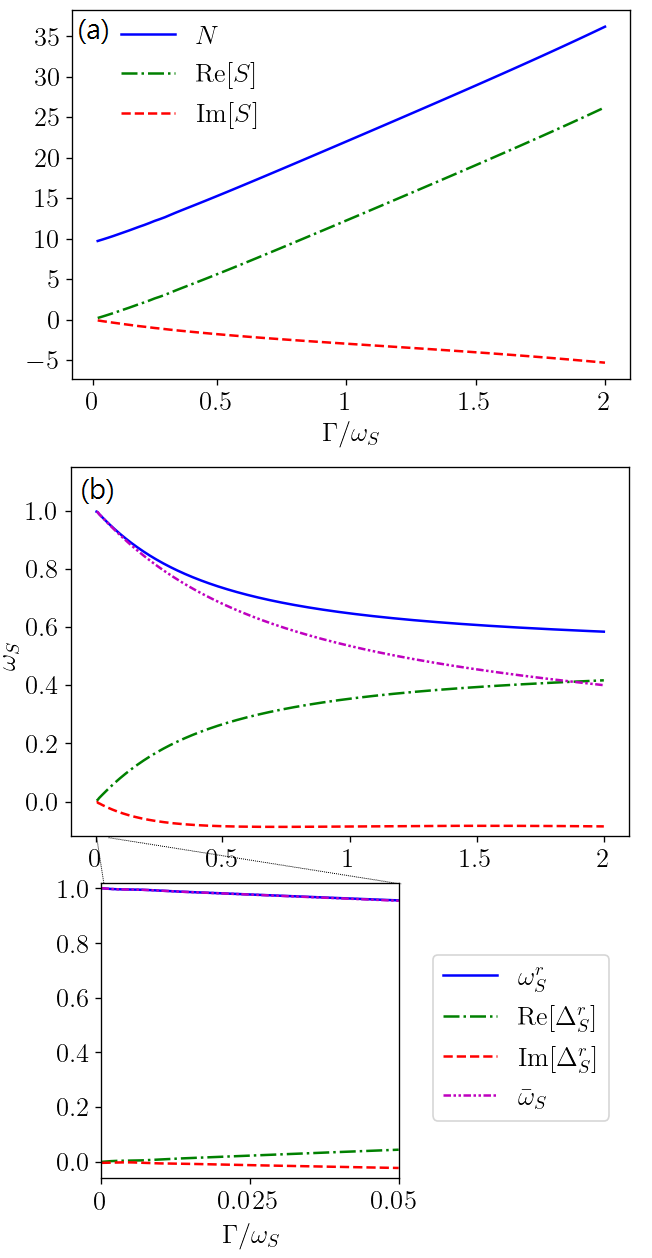
Figure 1: (Colour online) (a) The particle occupation $n$ and squeezing parameter $s$, and (b) the renormalized frequency and the renormalized pairing strength as functions of the coupling strength $\Gamma/\omega_{S}$ and its partial enlarged view that focuses on the weak coupling regime in the bottom plot. The temperature is set at $T=10\hbar\omega_{S}/k_{B}$ and the cutoff frequency is set as $\omega_{D}=20\omega_{S}$.

Note that the particle occupation of quantum Brownian motion containing pairing couplings does not simply obey the standard Bose-Einstein distribution. This is because both the energy frequency $\omega^{r}_{S}$ and the pairing strength $\Delta^{r}_{S}$ contributes to the particle occupation for quantum Brownian motion, as shown by Eq. (30a). In Eq. (16), we have given the solutions of particle occupation and squeezing from the total equilibrium state of the system plus its reservoir for arbitrary reservoir spectrum and arbitrary system-reservoir coupling. For a practical numerical calculation and without loss of generality, we consider here a Lorentz-Drude spectral density

$$J(\omega)\equiv 2\pi\sum\limits_{k}\left|V_{k}\right|^{2}\delta(\omega-\omega_{k})=\dfrac{\Gamma\omega\omega_{D}^{2}}{\omega^{2}+\omega_{D}^{2}},$$ (38)

which has been applied in many studies of quantum Brownian motion PH06 ; PH08 ; PH09 ; nega4 ; nega5 ; HC2 ; Grabert1 ; MF2 ; Grabert2 ; drude1 ; drude2 ; drude3 . The parameter $\omega_{D}$ is a cut-off frequency of the reservoir spectrum and $\Gamma$ represents the coupling strength between the system and reservoir.

We calculate the occupation $n$ and squeezing $s$ of the Brownian particle from Eq. (16) with the system-reservoir coupling characterized by Eq. (38). The numerical result of those as functions of the coupling strength $\Gamma/\omega_{S}$ are plotted in Fig. 1(a). It shows that the finite system-reservoir coupling can result in a non-trivial squeezing effect to the Brownian particle. Only in the weak-coupling limit $\Gamma/\omega_{S}\rightarrow 0$ does the value of the squeezing parameter approach to zero, rendering it negligible in comparison to the particle occupation. In Fig. 1(b), we plot the renormalized frequency $\omega_{S}^{r}$, the pairing strength $\Delta_{S}^{r}$ of the squeezing term, and the renormalized eigen-frequency $\bar{\omega}_{S}=\sqrt{|\omega_{S}^{r2}-|\Delta_{S}^{r}|^{2}|}$ as functions of the coupling strength $\Gamma/\omega_{S}$. It shows that increasing the system-reservoir coupling reduces the system frequency and generates the pairing energy. One can also find that when the system-reservoir coupling is very weak, the strength of the renormalized pairing energy $\Delta_{S}^{r}$ becomes significantly less than the renormalized system frequency $\omega_{S}^{r}$. It can be seen more clearly in its partial enlarged view below, where we focus on the part of weak-coupling regime ($\Gamma/\omega_{S}\leq 0.05$). It shows that the renormalized eigen-frequency $\bar{\omega}_{S}$ is almost the same with the renormalized frequency $\omega_{S}^{r}$ at weak coupling, while the effect of the pairing strength $\Delta_{S}^{r}$ is so weak that it can be neglected in the very weak-coupling limit. Thus, only in the weak-coupling limit, the renormalized Hamiltonian shown in Eq. (23) or Eq. (II) can be approximated to a harmonic oscillator with the renormalized frequency $\omega_{S}^{r}$ alone. Once one goes beyond the weak-coupling limit, the pairing energy becomes comparable to that of the renormalized frequency $\omega_{S}^{r}$. As a result, in the strong coupling, it is necessary to take into account the contribution of the pairing effect in Eq. (23) or the momentum-dependent potential shown in Eq. (II) for the calculations of all thermodynamic quantities.

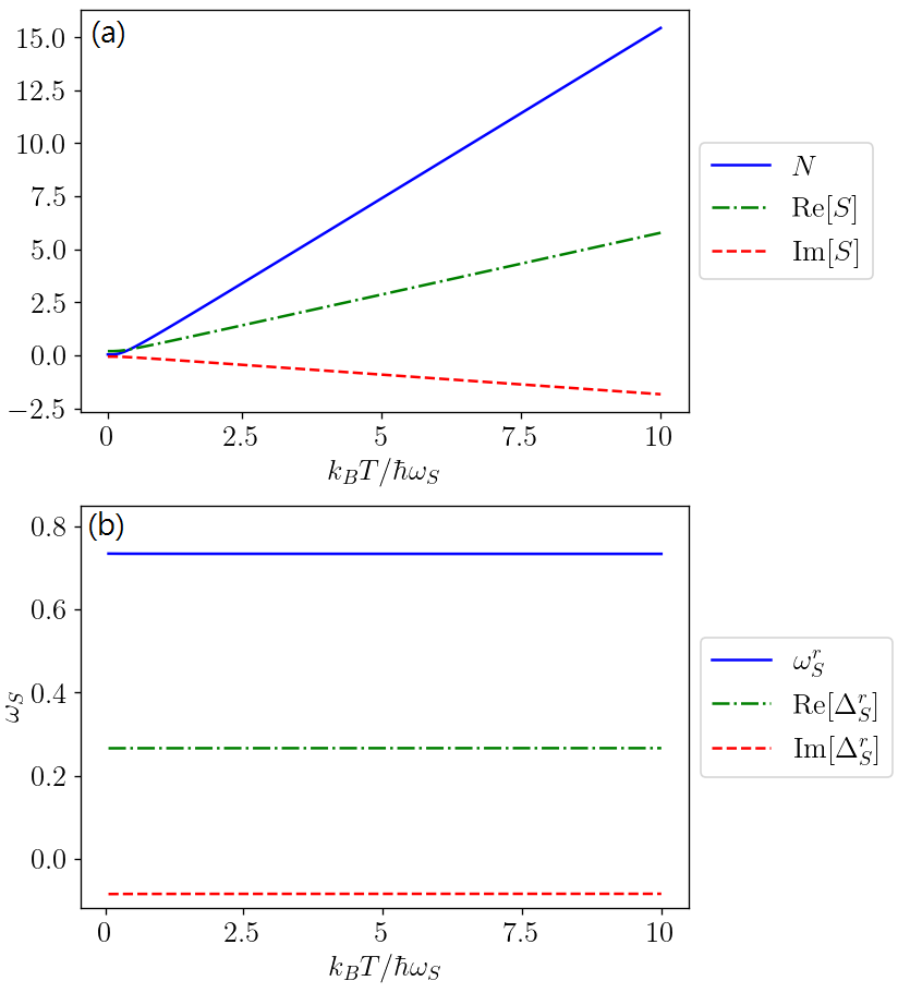
Figure 2: (Colour online) (a) The particle occupation and particle squeezing and (b) the renormalized frequency and the renormalized pairing strength as functions of temperature for coupling strength $\Gamma/\omega_{S}=0.5$. The latter two quantities are independent of temperature, as shown in Fig. (2)(b), so does the renormalized Hamiltonian Eq. (23) or Eq. (II).

In Fig. 2, we also present those physical quantities as functions of temperature $kT/\hbar\omega_{S}$. Figure 2(a) shows the monotonic variations of both the particle occupation $n$ and squeezing parameter $s$ as temperature increasing. Contrastingly, Fig. 2(b) reveals that both the renormalized frequency $\omega_{S}^{r}$ and pairing strength $\Delta_{S}^{r}$ remain unchanged with respect to the temperature vary, although they are calculated based on the temperature-dependent particle occupation $n$ and squeezing parameter $s$ through Eq. (19) and Eq. (24). This justifies our conclusion made in Sec. II that our renormalized Hamiltonian $H_{S}^{r}$ derived from the exact reduced density matrix of Eq. (22) is temperature independent, in contrast to the Hamiltonian of mean force introduced in previous works PH20 ; MF1 ; MF2 ; MF3 ; MF4 ; MF5 ; MF6 which is considered or assumed to be temperature-dependent.

III.2 The renormalized internal energy and heat capacity

III.2.1 The calculations with the exact reduced density matrix and the exact reduced partition function

The definition of the system internal energy beyond weak coupling has been debated for many years. In the literature, different definitions the internal energy give inconsistent results PH06 ; PH08 ; PH09 . We find that the inconsistency comes from the lack of the way to take into account all the renormalization effects induced from the system-reservoir coupling. With the exact solution of the reduced density matrix $\rho_{S}$ given by Eq. (22) [or Eq. (18)] and the renormalized Hamiltonian of Eq. (23), which encapsulates all the renormalization effects, the internal energy of the system can be defined unambiguously and self-consistently. The direct definition of the internal energy is given by

$$U_{H}\equiv \operatorname{Tr}_{S}[H_{S}^{r}\rho_{S}]$$

$$= \dfrac{1}{2M^{\prime}}\langle P^{2}\rangle+\dfrac{M^{\prime}}{2}\left(\omega_{S}^{r2}-\textrm{Re}[\Delta_{S}^{r}]^{2}\right)\langle X^{2}\rangle$$

$$+\dfrac{1}{2}\textrm{Im}[\Delta_{S}^{r}]\langle XP+PX\rangle$$

$$= \dfrac{\hbar}{2}\big{[}\omega_{S}^{r}(2n+1)+2\textrm{Re}[\Delta_{S}^{r}s]\big{]}$$ (39)

With the aid of Eq. (30a), the internal energy can be simpley expressed with the renormalized eigen-frequency $\bar{\omega}_{S}$ of the Bogoliubov quasi-particle,

$$U_{H}=\hbar\bar{\omega}_{S}\left(\dfrac{1}{\exp\left[\frac{\hbar\bar{\omega}_{S}}{k_{B}T}\right]-1}+\frac{1}{2}\right).$$ (40)

It shows that the internal energy can be expressed in terms of the renormalized eigen-frequency of the Bogoliubov quasi-particle which is no longer the original simple harmonic oscillator but a mixture of the original harmonic oscillator and all of particles in the reservoir, as shown by Eq. (27).

Alternatively, one can also define the internal energy from the partition function $Z_{S}^{r}$ of the renormalized Brownian particle, given by Eq. (II) or more specifically by Eq. (19c) which can be expressed further as

$$Z_{S}^{r} =\sqrt{n^{2}+n-|s|^{2}}=\dfrac{1}{2}\operatorname{csch}\left(\dfrac{\hbar\bar{\omega}_{S}}{2k_{B}T}\right).$$ (41)

Then using the well-known definition of the internal energy through the partition function, we obtain

$$U_{Z} \equiv-\dfrac{\partial}{\partial\beta}\ln(Z_{S}^{r})=\dfrac{1}{2}\hbar\bar{\omega}_{S}\coth\left(\dfrac{\hbar\bar{\omega}_{S}}{2k_{B}T}\right)$$

$$=\hbar\bar{\omega}_{S}\left(\dfrac{1}{\exp\left[\frac{\hbar\bar{\omega}_{S}}{k_{B}T}\right]-1}+\frac{1}{2}\right).$$ (42)

It shows that the internal energy $U_{Z}$ defined through the partition function of the renormalized Brownian particle is exactly the same as the internal energy $U_{H}$ defined by the renormalized Hamiltonian with the exact solution of the reduced density matrix, as shown in Eq. (40). In other words, the two different definitions of the internal energy agree with each other, unlike the previous works PH06 ; PH08 ; PH09 where they used an un-renormalized Hamiltonian and an incomplete partition function of the reduced system that result in the inconsistent solutions of the internal energy.

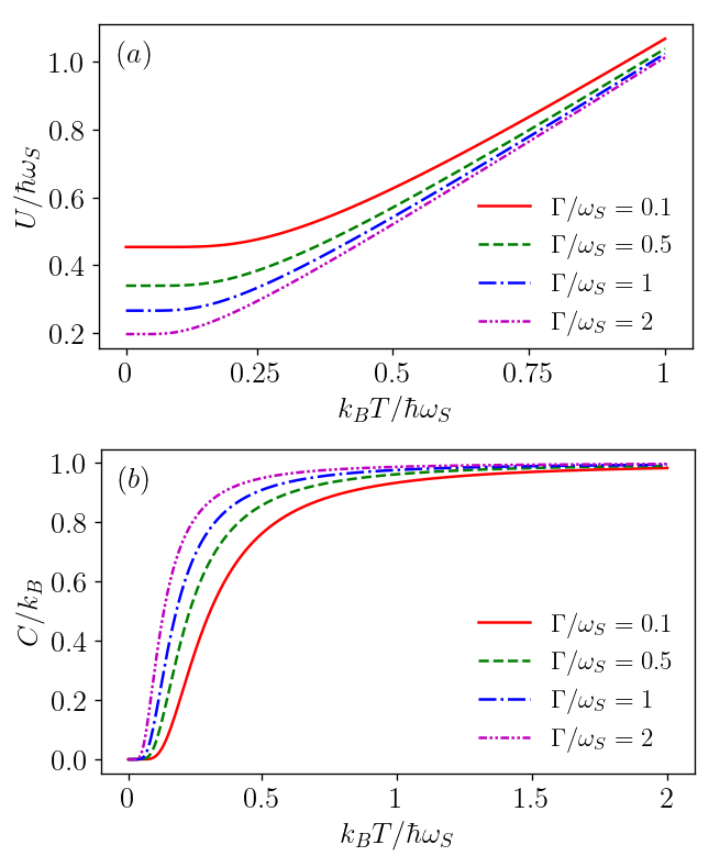
Figure 3: (Colour online) (a) The internal energy and (b) the heat capacity as a function of temperature with different coupling strength $\Gamma/\omega_{S}$, calculated from both the fully renormalized Hamiltonian with the exact reduced density matrix Eq. (III.2.1) and the renormalized partition function of Eq. (42), both give the same result.

With the self-consistent result of internal energy presented by Eq. (40) and Eq. (42), we can obtain the unique heat capacity

$$C\equiv\dfrac{\partial U}{\partial T}=\left[\dfrac{\hbar\bar{\omega}_{S}}{2k_{B}T}\operatorname{csch}\left(\dfrac{\hbar\bar{\omega}_{S}}{2k_{B}T}\right)\right]^{2}.$$ (43)

It is consistent with the results of the Einstein model for a single-mode quantum Brownian particle, except that the harmonic oscillator frequency is now given by the renormalized eigen-frequency of the Bogoliubov quasi-particle, which encapsulates all the renormalization effects of the system-reservoir coupling on the system, including the frequency shift and the induced pairing effect. The result of Eq. (43) is a monotonically increasing function of the ratio $k_{B}T/\hbar\bar{\omega}_{S}$, and obviously in no case does it lead to the negative heat capacity found in the literature PH06 ; PH08 ; PH09 ; nega4 ; nega5 . At low temperatures, it decreases to zero as $C\simeq(\frac{\hbar\bar{\omega}_{S}}{2k_{B}T})^{2}\exp(-\frac{\hbar\bar{\omega}_{S}}{k_{B}T})$, while it approaches to a constant $k_{B}$ at high temperatures.

In Fig. 3, we present the numerical results of the internal energy and the heat capacity as a function of the temperature with several different coupling strength. The internal energy as a function of temperature with the different ratio of $\Gamma/\omega_{S}$ is shown in Fig. 3(a). At very low temperature, the different coupling strengths make the internal energy significantly different. On the other hand, for the reservoir with the Drude-Lorentz spectral density, the renormalized eigen-frequency $\bar{\omega}_{S}=\sqrt{|\omega_{S}^{r2}-|\Delta_{S}^{r}|^{2}|}$ always decrease as the coupling strength $\Gamma/\omega_{S}$ increases, as shown in Fig. 1(b), Thus, the heat capacity will increase monotonically with the coupling strength increasing, as shown in Fig. 3(b) where the heat capacity as a function of temperature with the different ratio $\Gamma/\omega_{S}$ is presented. At high temperature, the internal energy and the heat capacity of Brownian particle approach to the classical limit, following the equipartition theorem, as one expected. In other words, a one-dimensional harmonic oscillator has the average energy $1\ k_{B}T$, and therefore its heat capacity is $1\ k_{B}$, as shown in Fig. 3(a) and Fig. 3(b) for high temperature, and the effects of the system-reservoir coupling become negligible. Thus, the thermodynamic solution of the quantum Brownian particle is consistently presented in our theory.

III.2.2 Comparing our results with previous works

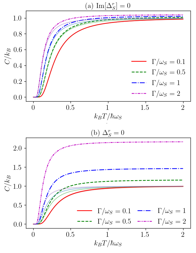
Figure 4: (Colour online) The heat capacity as a function of temperature with different coupling strength $\Gamma/\omega_{S}$. (a) The imaginary part of $\Delta_{S}^{r}$ is zero, namely the momentum-dependent potential in the renormalized Hamiltonian is ignored, and (b) both the imaginary part and the real part of $\Delta_{S}^{r}$ are zero, namely the squeezing effect is totally ignored. The light dotted lines are the fully renormalized results ($\textrm{Im}[\Delta_{S}^{r}]\neq 0$ and $\textrm{Re}[\Delta_{S}^{r}]\neq 0$) as given in Fig. 3(b), serving as a basis for comparison here.

In the preceding discussion, in order to unambiguously determining thermodynamic quantities in the framework of quantum thermodynamics, we have elucidated the necessity of taking into account all the renormalization effects on the Brownian particle Hamiltonian and partition function induced by the system-reservoir coupling. Now, we would like to compare our results with the results based on an incomplete-renormalized Hamiltonian and an incorrect partition function of the Brownian particle obtained in the previous works. Here the term ”incomplete-renormalized Hamiltonian” refers to the ignorance of the momentum-dependent potential (or the pairing effect) generated from the system-reservoir coupling in the previous works HC2 ; Grabert1 ; MF2 ; PH06 ; PH08 . The incorrect partition function corresponds to the thought which is widely used in the literature that the reservoir is large enough so its states should remain unchanged. Thus, the partition function for the Brownian particle was simply defined as the partition function of the total system divided by that of the reservoir: $Z_{S}=Z_{\rm tot}/Z_{E}$, where $Z_{E}\equiv\operatorname{Tr}_{E}[\exp(-\beta H_{E})]$, as used in many previous works PH06 ; PH08 ; PH09 ; PH20 ; nega4 ; nega5 ; HC2 ; MF1 ; MF2 ; MF3 ; MF4 ; MF5 ; MF6 ; Seifert16 ; Jarzynski17 . However, such widely used definition of the partition function of the subsystem is incorrect. Our derivation in Sec. II shows that the reservoir and the system will mutually influence each other, which non-negligibly change both the system and the reservoir states.

In Fig. 4(a), we plot the heat capacity for different coupling strengths calculated by the incomplete-renormalized Hamiltonian which ignores the momentum-dependent potential, as considered in Ref. HC2 ; Grabert1 ; MF2 . In Fig. 4(b), we also plot the heat capacity by enforcing both the real and imaginary parts of the renormalized pairing strength $\Delta_{S}^{r}$ in Eq. (III.2.1) so that not only the momentum-dependent potential energy is omitted, but also the oscillation frequency of the Brownian particle influenced by the thermal reservoir is not correctly renormalized, as considered in Ref. PH06 ; PH08 . We make a comparison with the results calculated from our theory, i.e., Fig. 3 and plot them by the light dotted lines in Fig. 4(a)-(b). The differences are significant as one can see in Fig. (4). In particular, in the strong coupling and high temperature regime, using the incomplete-renormalized Hamiltonian where the pairing terms (squeezing effect) are partially neglected [Fig. 4(a)] or completely neglected [Fig. 4(b)], it shows that the value of $C/k_{B}$ is larger than one, which is unphysical. Only in the weak coupling (e.g. $\Gamma=0.1\omega_{S}$), the heat capacity calculated with the incomplete renormalized Hamiltonian HC2 ; Grabert1 ; MF2 ; PH06 ; PH08 gives almost the same value obtained from our derivation (see the red line in Fig. (4)). This is because in the weak coupling, the effect of the pairing strength $\Delta_{S}^{r}$ is very weak so that the renormalized eigen-frequency $\bar{\omega}_{s}$ can be approximated as the renormalized frequency $\omega_{S}^{r}$, as shown in Fig. 1(b). In the strong coupling, the renormalized pairing strength $\Delta_{S}^{r}$ as well as the squeezing $s$ become important, as shown in Fig. 2(a). While the effect of particle squeezing is amplified as the temperature increases due to the increase of the occupancy number in the quantum Brownian motion. Thus, the incomplete renormalized Hamiltonian of the Brownian particle leads to the unphysical results of the heat capacity at high temperature which are expected to approach to the classical limit. This indicates that a correct renormalized Hamiltonian is significantly important to correctly define quantum thermodynamical quantities in the strong coupling.

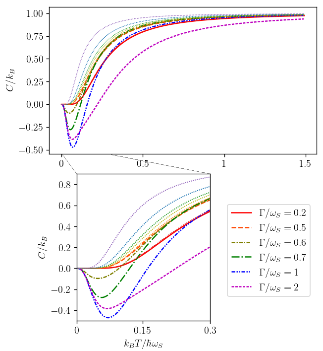
Figure 5: (Colour online) The heat capacity as a function of temperature with different coupling strength $\Gamma/\omega_{S}$, calculated based on the incomplete-renormalized partition function $Z_{S}=Z_{tot}/Z_{E}$. The light dotted-lines are the results calculated based on the renormalized partition function $Z_{S}^{r}$ given in Fig. 3(b), serving as a basis for comparison here.

On the other hand, we also numerically demonstrate why it gives the negative heat capacity in the previous investigations of quantum Brownian motion PH06 ; PH08 ; PH09 ; nega4 ; nega5 . We find that the negative heat capacity comes from the naive assumption of the reduced partition function $Z_{S}\equiv Z_{\rm{tot}}/Z_{E}$ which has been used widely in the literature because it is commonly thought of the reservoir being larger enough so that the reservoir states remain unchanged even if the system strongly couples the reservoir. As we have shown in this work, this naive assumption is incorrect. The exactly renormalized partition function $Z_{S}^{r}$ for the quantum Brownian motion is given by Eq. (II) which cannot be written as $Z^{r}_{S}=Z_{\rm{tot}}/Z_{E}$. Recall the relation between the internal energy and partition function $U=-\frac{\partial}{\partial\beta}\ln(Z)$ shown in the first line of Eq. (42), if one uses the incorrect partition function $Z_{S}=Z_{\rm{tot}}/Z_{E}$, the corresponding internal energy is given by

$$U =-\frac{\partial}{\partial\beta}[\ln(Z_{\rm{tot}})-\ln(Z_{E})]$$

$$=-\frac{\partial}{\partial\beta}\left[\ln\left(\operatorname{Tr}_{\rm{tot}}e^{-\beta H_{\rm{tot}}}\right)-\ln\left(\operatorname{Tr}_{\rm{E}}e^{-\beta H_{E}}\right)\right].$$ (44)

Then the heat capacity $C\equiv\dfrac{\partial U}{\partial T}$ using this incorrect internal energy will give the negative values of $C$ in the strong coupling, as have been numerically shown in the early studies PH06 ; PH08 ; PH09 ; nega4 ; nega5 , and as we also plot in Fig. 5. It becomes more obvious in the partially enlarged plot in the low temperature regime in Fig. 5, where one can clearly see the negative heat capacity for strong couplings $\Gamma\geq 0.6\,\omega_{S}$. In Fig. 5, we also plot the heat capacity based on the renormalized partition function $Z^{r}_{S}$ of by Eq. (II) with the light dotted lines [also see Fig. 3(b)] for a comparison. It shows that the negative heat capacity of the quantum Brownian motion is a consequence of the use of the incorrect partition function. Thus, despite the reservoir is typically and significantly larger than the system, its states are still changed due to the influence from the system in the strong coupling, leading to the necessity to correct the renormalization of the partition function and Hamiltonian of the system in a correct way. Only in the weak coupling regime, the heat capacities calculated based on $Z_{S}$ and $Z_{S}^{r}$ are nearly identical. Therefore, the claimed anomalous phenomenon of negative heat capacity under strong coupling in the literature is, in fact, a misinterpretation resulting from the incorrect renormalization of the partition function.

IV Conclusion

In conclusion, we apply our nonperturbative renormalization theory to the quantum Brownian motion model. We traced over exactly all the reservoir states through the Gaussian integral approach in coherent state representation. According to the result of these rigorous derivations, we find that the widely used definition of the reduced system partition function $Z_{S}\equiv Z_{\rm{tot}}/Z_{E}$ is not valid for strong couplings. Our solution indicates that in the strong coupling, even if the thermal reservoir being significantly larger (containing much more degrees of freedom) than the system, its states are still influenced and nontrivially altered by the system through the system-reservoir coupling. This also implies that the Hamiltonian of mean force, widely used to describe quantum systems non-weakly coupled to the environment, is actually not valid in the strong coupling. Furthermore, using the assistance of faithful representation group theory, we successfully rearrange the order of operators and derive the exact reduced density matrix which can be expressed as the standard Gibbs state in terms of the fully renormalized system Hamiltonian, given by Eqs. (22) and (23). The renormalization effects arisen from the system-reservoir coupling not only shifts the frequency $\omega_{S}^{r}$ of the renormalized Brownian particle, but also generates the pairing energies $\Delta_{S}^{r}aa+\Delta_{S}^{r*}a^{\dagger}a^{\dagger}$ into the renormalized Hamiltonian. The existence of paired term inevitably generates a momentum-dependent potential.

As a consequence of the presence of pairing energies induced in the renormalized Hamiltonian, the relation between particle occupation $n$ and renormalized frequency $\omega_{S}^{r}$ of the Brownian particle cannot simply obey the Bose–Einstein distribution function. Based on the exact solutions of reduced density matrix and the fully renormalized Hamiltonian, we find an extended distribution function that describes the relation between particle occupation $n$ and particle squeezing $s$ in terms of the renormalized frequency $\omega_{S}^{r}$ and the renormalized pairing strength $\Delta_{S}^{r}$, as given by Eq. (30). Only after applying a Bogoliubov transformation to diagonalize the renormalized Brownian motion, allowing it to be represented as quasi-particles within a harmonic potential in the new coordinates. Then the particle occupation of the Bogoliubov quasi-particle obey the conventional Bose–Einstein distribution with the renormalized eigen-frequency $\bar{\omega}_{S}$ given by Eq. (27). We also show that the fully renormalized Hamiltonian is temperature independent.

We study further the internal energy and heat capacity based on the exact reduced density matrix and the renormalized system Hamiltonian. We obtain the consistent internal energy for the Brownian particle from the two different definitions based on the renormalized Hamiltonian and based on the renormalized partition function, respectively. The controversial results of the heat capacity used these two different definitions obtained in PH06 ; PH08 ; PH09 are resolved. We also find that the corresponding heat capacity of the Brownian particle modeled as a harmonic oscillator agrees with the results of the Einstein model, with the distinction that the oscillation frequency is replaced by the renormalized eigen-frequency of the Bogoliubov quasi-particle. Moreover, we numerically compare our results with those obtained based on the incomplete-renormalized partition function and incomplete-renormalized Hamiltonian, as considered in the literature. We found that the lack of the paring strength term in the incomplete-renormalized Hamiltonian leads to the failure of the heat capacity for reproducing the classical limit at high temperature. More importantly, the incomplete renormalization of the partition function that results in the negative heat capacity in the low-temperature regime in the literature is also resolved. These could potentially provide a reliable foundation for studying the quantum thermodynamics without being constrained by ambiguous definitions of thermodynamic quantities in quantum mechanics.

Appendix A Derivation of the exact reduced density matrix using the faithful matrix representation

In this appendix, we present the derivation of the exact reduced density matrix of the Brownian particle. We start from the particle number representation of the Hamiltonian for quantum Brownian motion as shown by Eq. (II). This Hamiltonian is indeed a linear function of the generators of the symplectic Lie group $Sp(2(k+1)+2)$ for the mutilmode bosonic systems (see Sec. D1 of Ref. group ), and $k$ is the number of modes in the reservoir. Because the total system is assumed to be in equilibrium, the density matrix of the total system should be able to be represented as

$$\rho_{\rm{tot}} =\dfrac{1}{Z_{\rm{tot}}}e^{-\beta H_{\rm{tot}}}$$

$$=\dfrac{1}{Z_{\rm{tot}}}\exp\left\{-\hbar\beta\left[\frac{\omega_{S}}{2}(a^{\dagger}a+aa^{\dagger})+\sum_{k}\frac{\omega_{k}}{2}(b^{\dagger}b+bb^{\dagger})+\sum_{k}V_{k}(a^{\dagger}+a)(b^{\dagger}+b)+\lambda\right]\right\},$$ (45)

where $\lambda=-\dfrac{1}{2}\Big{(}\omega_{S}+\sum_{k}\omega_{k}\Big{)}$. The faithful matrix representation group of the algebra of the total system gives the operator in terms of matrix as follows:

$$\frac{\omega_{S}}{2}(a^{\dagger}a+aa^{\dagger})+\sum_{k}\frac{\omega_{k}}{2}(b^{\dagger}b+bb^{\dagger})+\sum_{k}V_{k}(a^{\dagger}+a)(b^{\dagger}+b)+\lambda=\begin{pmatrix}0&0&\bm{0}&\bm{0}&0&0\\ 0&\omega_{S}&\bm{V}_{S\bm{E}}&\bm{\bar{V}}_{S\bm{E}}&0&0\\ \bm{0}&\bm{V}^{\dagger}_{S\bm{E}}&\bm{\omega_{E}}&\bm{0}&\bm{V}^{\dagger}_{S\bm{E}}&\bm{0}\\[2.84526pt] \bm{0}&-\bm{\bar{V}}^{\dagger}_{S\bm{E}}&\bm{0}&-\bm{\tilde{\omega}_{E}}&-\bm{\bar{V}}^{\dagger}_{S\bm{E}}&\bm{0}\\ 0&0&-\bm{V}_{S\bm{E}}&-\bm{\bar{V}}_{S\bm{E}}&-\omega_{S}&0\\ \lambda&0&\bm{0}&\bm{0}&0&0\end{pmatrix},$$ (46)

where

$$\bm{\omega_{E}}=\!\begin{pmatrix}&\omega_{k_{1}}&&&\\[-5.69054pt] &&\omega_{k_{2}}&&\mbox{\Huge 0}\\ &\mbox{\Huge 0}&&&\ddots\end{pmatrix}\!,\ \bm{\widetilde{\omega}_{E}}=\!\begin{pmatrix}&\ddots&&&\mbox{\Huge 0}\\ &&&\omega_{k_{2}}&\\[-5.69054pt] &\mbox{\Huge 0}&&&\omega_{k_{1}}\end{pmatrix}\!,\ \bm{V}_{S\bm{E}}=\begin{pmatrix}V_{k_{1}}&V_{k_{2}}&\cdots\end{pmatrix},\ \bm{\bar{V}}_{S\bm{E}}=\begin{pmatrix}\cdots&V_{k_{2}}&V_{k_{1}}\end{pmatrix}.$$ (47)

Then the faithful matrix representation of the density matrix of the total system can be expressed as

$$\rho_{\rm{tot}}=\begin{pmatrix}1&\bm{0}&0\\ \bm{0}&\exp\left[\begin{array}[]{cc}\bm{D}&\bm{R}\\ -\bm{\hat{R}}&-\bm{\tilde{D}}\end{array}\right]&\bm{0}\\ 2\ln Z_{\rm{tot}}&\bm{0}&1\end{pmatrix},\ \bm{D}=-\dfrac{\hbar\beta}{2}\begin{pmatrix}\omega_{S}&\bm{V}_{S\bm{E}}\\ \bm{V}_{S\bm{E}}^{\dagger}&\bm{\omega_{E}}\end{pmatrix},\ \bm{R}=-\dfrac{\hbar\beta}{2}\begin{pmatrix}\bm{\bar{V}}_{S\bm{E}}&0\\ \bm{0}&\bm{V}_{S\bm{E}}^{\dagger}\end{pmatrix},$$ (48)

where the ”tilde” indicates reflection in the minor diagonal, and the ”hat” indicates reflection in the major diagonal.

Now we rearrange the ordering of the exponential operator products of Eq. (45) as

$$\rho_{\rm{tot}}= \dfrac{1}{Z_{\rm{tot}}}\exp\left[\dfrac{1}{2}\begin{pmatrix}a^{\dagger}&\bm{b^{\dagger}}\end{pmatrix}\begin{pmatrix}\Pi_{SS}&\bm{\Pi}_{S\bm{E}}\\ \bm{\Pi}_{S\bm{E}}^{*}&\bm{\Pi_{EE}}\end{pmatrix}\begin{pmatrix}a^{\dagger}\\ \bm{b^{\dagger}}\end{pmatrix}\right]$$

$$\times\exp\left[\dfrac{1}{2}\begin{pmatrix}a^{\dagger}&\bm{b^{\dagger}}\end{pmatrix}\begin{pmatrix}\Omega^{{}_{0}}_{SS}&\bm{\Omega^{{}_{0}}}_{S\bm{E}}\\ \bm{\Omega}_{S\bm{E}}^{{}_{\bm{0}}*}&\bm{\Omega^{{}_{0}}_{EE}}\end{pmatrix}\begin{pmatrix}a\\ \bm{b}\end{pmatrix}+\dfrac{1}{2}\begin{pmatrix}a&\bm{b}\end{pmatrix}\begin{pmatrix}\Omega^{{}_{0}}_{SS}&\bm{\Omega}^{{}_{\bm{0}}*}_{S\bm{E}}\\ \bm{\Omega^{{}_{0}}}_{S\bm{E}}&\bm{\Omega^{{}_{0}}}_{\bm{EE}}\end{pmatrix}\begin{pmatrix}a^{\dagger}\\ \bm{b^{\dagger}}\end{pmatrix}\right]$$

$$\times\exp\left[\dfrac{1}{2}\begin{pmatrix}a&\bm{b}\end{pmatrix}\begin{pmatrix}\Pi_{SS}&\bm{\Pi}_{S\bm{E}}^{*}\\ \bm{\Pi}_{S\bm{E}}&\bm{\Pi_{EE}}\end{pmatrix}\begin{pmatrix}a\\ \bm{b}\end{pmatrix}\right].$$ (49)

Its faithful matrix representation is explicitly given by

$$\rho_{\rm{tot}}=\begin{pmatrix}1&\bm{0}&\bm{0}&0\\ \bm{0}&\bm{\Omega}-\,\bm{\Pi}\,\bm{\tilde{\Omega}}^{-1}\bm{\hat{\Pi}}&\bm{\Pi}\,\bm{\tilde{\Omega}}^{-1}&\bm{0}\\ \bm{0}&-\bm{\tilde{\Omega}}^{-1}\bm{\hat{\Pi}}&\bm{\tilde{\Omega}}^{-1}&\bm{0}\\ 2\ln Z_{\rm{tot}}&\bm{0}&\bm{0}&1\end{pmatrix},\$$ (50)

where

$$\bm{\Pi}=\begin{pmatrix}\Pi_{SS}&\bm{\Pi}_{S\bm{E}}\\ \bm{\Pi}_{S\bm{E}}^{*}&\bm{\Pi_{EE}}\end{pmatrix},\ \bm{\Omega}=\begin{pmatrix}\Omega_{SS}&\bm{\Omega}_{S\bm{E}}\\ \bm{\Omega}_{S\bm{E}}^{*}&\bm{\Omega_{EE}}\end{pmatrix}=\exp\left[\begin{pmatrix}\Omega^{{}_{0}}_{SS}&\bm{\Omega^{{}_{0}}}_{S\bm{E}}\\ \bm{\Omega}_{S\bm{E}}^{{}_{\bm{0}}*}&\bm{\Omega^{{}_{0}}_{EE}}\end{pmatrix}\right].$$ (51)

By comparing Eq. (48) and Eq. (50), one can find that

$$\bm{\tilde{\Omega}}=\left\{\begin{pmatrix}\bm{0}&\bm{I}\end{pmatrix}\exp\left[\begin{pmatrix}\bm{D}&\bm{R}\\ -\bm{\hat{R}}&-\bm{\tilde{D}}\end{pmatrix}\right]\begin{pmatrix}\bm{0}\\ \bm{I}\end{pmatrix}\right\}^{-1},\ \bm{\Pi}=\left\{\begin{pmatrix}\bm{I}&\bm{0}\end{pmatrix}\exp\left[\begin{pmatrix}\bm{D}&\bm{R}\\ -\bm{\hat{R}}&-\bm{\tilde{D}}\end{pmatrix}\right]\begin{pmatrix}\bm{0}\\ \bm{I}\end{pmatrix}\right\}\bm{\tilde{\Omega}},$$ (52)

as given in Eq. (7). The coherent state representation of the density matrix of the total system can be easily obtained

$$\langle z_{S},\bm{z_{E}}|\rho_{\rm{tot}}|z_{S}^{\prime},\bm{z_{E}}\rangle= \dfrac{1}{Z_{\rm{tot}}}\exp\left[\dfrac{1}{2}\bm{z^{\dagger}}\bm{\Pi}\bm{z^{*}}+\dfrac{1}{2}\bm{z^{\prime T}}\bm{\Pi^{*}}\bm{z^{\prime}}\right]$$

$$\times\left\langle z_{S},\bm{z_{E}}\left|\exp\left[\begin{pmatrix}a^{\dagger}&\bm{b^{\dagger}}\end{pmatrix}\begin{pmatrix}\Omega^{{}_{0}}_{SS}&\bm{\Omega^{{}_{0}}}_{S\bm{E}}\\ \bm{\Omega}_{S\bm{E}}^{{}_{\bm{0}}*}&\bm{\Omega^{{}_{0}}_{EE}}\end{pmatrix}\begin{pmatrix}a\\ \bm{b}\end{pmatrix}+\dfrac{1}{2}\operatorname{Tr}\begin{pmatrix}\Omega^{{}_{0}}_{SS}&\bm{\Omega}^{{}_{\bm{0}}*}_{S\bm{E}}\\ \bm{\Omega^{{}_{0}}}_{S\bm{E}}&\bm{\Omega^{{}_{0}}}_{\bm{EE}}\end{pmatrix}\right]\right|z_{S}^{\prime},\bm{z_{E}}\right\rangle$$

$$= \dfrac{1}{Z_{\rm{tot}}}\exp\left[\dfrac{1}{2}\operatorname{Tr}\ln(\bm{\Omega})\right]\exp\left[\bm{z^{\dagger}}\bm{\Omega}\bm{z^{\prime}}+\dfrac{1}{2}\bm{z^{\dagger}}\bm{\Pi}\bm{z^{*}}+\dfrac{1}{2}\bm{z^{\prime T}}\bm{\Pi^{*}}\bm{z^{\prime}}\right]$$

$$= \dfrac{\sqrt{\det\bm{\Omega}}}{Z_{\rm tot}}\exp\!\left[\dfrac{1}{2}\begin{pmatrix}\bm{z^{\dagger}}&\bm{z^{\prime T}}\end{pmatrix}\!\!\begin{pmatrix}\bm{\Omega}&\bm{\Pi}\\ \bm{\Pi^{*}}&\bm{\Omega^{*}}\end{pmatrix}\!\!\begin{pmatrix}\bm{z^{\prime}}\\ \bm{z^{*}}\end{pmatrix}\!\right],$$ (53)

as given by Eq. (5).

Taking the trace over all the reservoir modes, we obtain the reduced density matrix of the Brownian particle in the coherent state representation

$$\langle z_{S}|\rho_{S}|z^{\prime}_{S}\rangle= \int d\mu(\bm{z_{E}})\langle z_{S},\bm{z_{E}}|\rho_{\rm{tot}}|z_{S}^{\prime},\bm{z_{E}}\rangle$$

$$= \dfrac{\sqrt{\det\bm{\Omega}}}{Z_{\rm{tot}}}\int d\mu(\bm{z_{E}})\exp\left[\dfrac{1}{2}\begin{pmatrix}\bm{z^{\dagger}}&\bm{z^{\prime T}}\end{pmatrix}\begin{pmatrix}\bm{\Omega}&\bm{\Pi}\\ \bm{\Pi^{*}}&\bm{\Omega^{*}}\end{pmatrix}\begin{pmatrix}\bm{z^{\prime}}\\ \bm{z^{*}}\end{pmatrix}\right]$$ (54)

where $d\mu(\bm{z_{E}})=\prod\limits_{j}dz_{j}^{*}dz_{j}e^{-|z_{j}|^{2}}$. The Gaussian integral $\int d\mu(\bm{\xi})e^{\bm{\xi^{\dagger}}\cdot\bm{\Theta}\cdot\bm{\xi}+\bm{\eta^{\dagger}}\cdot\bm{\xi}+\bm{\xi^{\dagger}}\cdot\bm{\eta^{\prime}}}=||\bm{1}-\bm{\Theta}||e^{\bm{\eta^{\dagger}}\cdot(\bm{1}-\bm{\Theta})^{-1}\cdot\bm{\eta^{\prime}}}$ can be generalized to the system with pairing terms

$$\int d\mu(\bm{\xi})e^{\bm{\xi^{*}}\bm{\Theta}\bm{\xi}+\bm{\eta^{*}}\bm{\xi}+\bm{\xi^{*}}\bm{\eta^{\prime}}+\frac{1}{2}\bm{\xi^{*}}\bm{\mathcal{P}^{\prime}}\bm{\xi^{\dagger}}+\frac{1}{2}\bm{\xi^{T}}\bm{\mathcal{P}^{*}}\bm{\xi}}= \left\|\bm{1}-\bm{\Theta}\right\|^{-1/2}\left\|\bm{1}-\bm{\Phi}\right\|^{-1/2}\exp\left[\bm{\eta^{*}}(\bm{1}-\bm{\Phi})^{-1}\bm{\eta^{\prime}}\right]$$

$$\times\exp\left[\frac{1}{2}\bm{\eta^{*}}(\bm{1}-\bm{\Phi})^{-1}\bm{\mathcal{P}^{\prime}}(\bm{1}-\bm{\Theta^{T}})^{-1}\bm{\eta^{\dagger}}\right]$$

$$\times\exp\left[\frac{1}{2}\bm{\eta^{\prime T}}(\bm{1}-\bm{\Theta^{T}})^{-1}\bm{\mathcal{P}^{*}}(\bm{1}-\bm{\Phi})^{-1}\bm{\eta^{\prime}}\right]$$ (55)

where $\bm{\Phi}=\bm{\Theta}+\bm{\mathcal{P}^{\prime}}(\bm{1}-\bm{\Theta^{T}})^{-1}\bm{\mathcal{P}^{*}}$. By rewriting it in matrix form, the above equation can be reduced as

$$\int d\mu(\bm{\xi})\exp\left[\frac{1}{2}\begin{pmatrix}\bm{\xi^{*}}&\bm{\xi^{T}}\end{pmatrix}\begin{pmatrix}\bm{\Theta}&\bm{\mathcal{P}^{\prime}}\\ \bm{\mathcal{P}^{*}}&\bm{\Theta^{\dagger}}\end{pmatrix}\begin{pmatrix}\bm{\xi}\\ \bm{\xi^{\dagger}}\end{pmatrix}+\begin{pmatrix}\bm{\xi^{*}}&\bm{\xi^{T}}\end{pmatrix}\begin{pmatrix}\bm{\eta^{\prime}}\\ \bm{\eta^{\dagger}}\end{pmatrix}\right]$$

$$=\left\|\bm{1}-\bm{\Theta}\right\|^{-1/2}\left\|\bm{1}-\bm{\Phi}\right\|^{-1/2}\exp\left[\frac{1}{2}\begin{pmatrix}\bm{\eta^{*}}&\bm{\eta^{\prime T}}\end{pmatrix}\begin{pmatrix}(\bm{1}-\bm{\Phi})^{-1}&(\bm{1}-\bm{\Phi})\bm{\mathcal{P}}(\bm{1}-\bm{\Theta^{\dagger}})^{-1}\\ (\bm{1}-\bm{\Theta^{\dagger}})^{-1}\bm{\mathcal{P}^{*}}(\bm{1}-\bm{\Phi})^{-1}&(\bm{1}-\bm{\Phi^{T}})^{-1}\end{pmatrix}\begin{pmatrix}\bm{\eta^{\prime}}\\ \bm{\eta^{\dagger}}\end{pmatrix}\right]$$

$$=\left\|\bm{1}-\begin{pmatrix}\bm{\Theta}&\bm{\mathcal{P}^{\prime}}\\ \bm{\mathcal{P}^{*}}&\bm{\Theta^{\dagger}}\end{pmatrix}\right\|^{-1/2}\exp\left\{\frac{1}{2}\begin{pmatrix}\bm{\eta^{*}}&\bm{\eta^{\prime T}}\end{pmatrix}\left[\bm{1}-\begin{pmatrix}\bm{\Theta}&\bm{\mathcal{P}^{\prime}}\\ \bm{\mathcal{P}^{*}}&\bm{\Theta^{\dagger}}\end{pmatrix}\right]^{-1}\begin{pmatrix}\bm{\eta^{\prime}}\\ \bm{\eta^{\dagger}}\end{pmatrix}\right\}$$ (56)

By applying this generalized Gaussian integral to the integral in Eq. (A), we obtain

$$\langle z_{S}|\rho_{S}|z^{\prime}_{S}\rangle= \dfrac{\sqrt{\det\bm{\Omega}}}{Z_{\rm{tot}}}\left\|\bm{1}-\begin{pmatrix}\bm{\Omega_{EE}}&\bm{\Pi_{EE}}\\ \bm{\Pi_{EE}^{*}}&\bm{\Omega^{*}_{EE}}\end{pmatrix}\right\|^{-1/2}\exp\left[\dfrac{1}{2}\begin{pmatrix}z_{S}^{*}&z_{S}^{\prime}\end{pmatrix}\begin{pmatrix}\Omega_{SS}&\Pi_{SS}\\ \Pi_{SS}^{*}&\Omega_{SS}\end{pmatrix}\begin{pmatrix}z_{S}^{\prime}\\ z_{S}^{*}\end{pmatrix}\right]$$

$$\times\exp\left\{\dfrac{1}{2}\begin{pmatrix}z_{S}^{*}&z_{S}^{\prime}\end{pmatrix}\begin{pmatrix}\bm{\Omega}_{S\bm{E}}&\bm{\Pi}_{S\bm{E}}\\ \bm{\Pi}_{S\bm{E}}^{*}&\bm{\Omega}^{*}_{S\bm{E}}\end{pmatrix}\left[\bm{1}-\begin{pmatrix}\bm{\Omega_{EE}}&\bm{\Pi_{EE}}\\ \bm{\Pi_{EE}^{*}}&\bm{\Omega^{*}_{EE}}\end{pmatrix}\right]^{-1}\begin{pmatrix}\bm{\Omega}_{\bm{E}S}&\bm{\Pi}_{\bm{E}S}\\ \bm{\Pi}_{\bm{E}S}^{*}&\bm{\Omega}^{*}_{\bm{E}S}\end{pmatrix}\begin{pmatrix}z_{S}^{\prime}\\ z_{S}^{*}\end{pmatrix}\right\}$$

$$= \dfrac{1}{Z^{r}_{S_{0}}}\exp\left[\dfrac{1}{2}\begin{pmatrix}z_{S}^{*}&z_{S}^{\prime}\end{pmatrix}\begin{pmatrix}\Omega_{S}&\Pi_{S}\\ \Pi_{S}^{*}&\Omega_{S}\end{pmatrix}\begin{pmatrix}z_{S}^{\prime}\\ z_{S}^{*}\end{pmatrix}\right].$$ (57)

This is the result of Eq. (II). Furthermore, the correlation functions $n=\operatorname{Tr}[a^{\dagger}a\rho_{S}]$ and $s=\operatorname{Tr}[aa\rho_{S}]$ can also easily be calculated in terms of the Gaussian kernel element by using the same generalized Gaussian integral in the coherent state presentation,

$$\begin{pmatrix}n&s\\ s^{*}&h\end{pmatrix} \equiv\begin{pmatrix}\langle a^{\dagger}a\rangle&\langle aa\rangle\\ \langle a^{\dagger}a^{\dagger}\rangle&\langle aa^{\dagger}\rangle\end{pmatrix}$$

$$=\dfrac{1}{(1-\Omega_{S})^{2}-|\Pi_{S}|^{2}}\begin{pmatrix}\Omega_{S}(1-\Omega_{S})+|\Pi_{S}|^{2}&\Pi_{S}\\ \Pi_{S}^{*}&1-\Omega_{S}\end{pmatrix},$$ (58)

which gives the results of Eq. (16).

In order to find the reduced density matrix in an operator form, we use the same technique of the faithful matrix representation of group theory group . The above reduced density matrix in the coherent state representation can be rewritten as

$$\langle z_{S}|\rho_{S}|z_{S}^{\prime}\rangle= \dfrac{1}{Z_{S_{0}}^{r}}e^{\frac{1}{2}\Pi_{2}(z^{*}_{S})^{2}+z^{*}_{S}\Omega_{S}z^{\prime}_{S}+\frac{1}{2}\Pi^{*}_{S}(z^{\prime}_{S})^{2}}$$

$$= \dfrac{e^{-\gamma}}{Z_{S_{0}}^{r}}\langle z_{S}|e^{\alpha a^{\dagger 2}}e^{\gamma(a^{\dagger}a+aa^{\dagger})}e^{\alpha^{*}a^{2}}|z_{S}^{\prime}\rangle$$ (59)

Thus, we obtain

$$\rho_{S}=\dfrac{1}{Z_{S}^{r}}e^{\alpha a^{\dagger 2}}e^{\gamma(a^{\dagger}a+aa^{\dagger})}e^{\alpha^{*}a^{2}},$$ (60)

where

$$\alpha=\dfrac{\Pi_{S}}{2}=\dfrac{s}{2[(1+n)^{2}-|s|^{2}]}$$ (61a)

$$\gamma=\ln\sqrt{\Omega_{S}}=\ln\sqrt{1-\dfrac{1+n}{(1+n)^{2}-|s|^{2}}}$$ (61b)

$$Z_{S}^{r}=e^{\gamma}Z^{r}_{S_{0}}=\sqrt{\dfrac{\Omega_{S}}{(1-\Omega_{S})^{2}-|\Pi_{S}|^{2}}}=\sqrt{n^{2}+n-|s|^{2}}$$ (61c)

Furthermore, using the Baker-Campbell-Hausdroff formula of the group $H_{6}$ group , Eq. (A) can be expressed as

$$\rho_{S}=\dfrac{1}{Z_{S}^{r}}\exp\left[\eta(a^{\dagger}a+aa^{\dagger})+\delta^{*}a^{\dagger 2}+\delta a^{2}\right].$$ (62)

Using the faithful matrix representation again, we can determine the coefficients $\eta$ and $\delta$:

$$\dfrac{1}{Z_{S}^{r}}e^{\eta(a^{\dagger}a+aa^{\dagger})+\delta^{*}a^{\dagger 2}+\delta a^{2}}=\begin{pmatrix}1&0&0&0\\ 0&\cosh\theta+\frac{2\eta}{\theta}\sinh\theta&\frac{2\delta^{*}}{\theta}\sinh\theta&0\\ 0&-\frac{2\delta}{\theta}\sinh\theta&\cosh\theta-\frac{2\eta}{\theta}\sinh\theta&0\\ 2\ln Z_{S}^{r}&0&0&1\end{pmatrix},$$ (63)

where $\theta=2\sqrt{\left|\eta^{2}-|\delta|^{2}\right|}$. Comparing it to the faithful matrix representation of the reduced density matrix

$$\dfrac{1}{Z_{S}^{r}}e^{\alpha a^{\dagger 2}}e^{\gamma(a^{\dagger}a+aa^{\dagger})}e^{\alpha^{*}a^{2}} =\begin{pmatrix}1&0&0&0\\ 0&\Omega_{S}-|\Pi_{S}|^{2}\Omega_{S}^{-1}&\Pi_{S}\Omega_{S}^{-1}&0\\ 0&-\Pi^{*}_{S}\Omega_{S}^{-1}&\Omega_{S}^{-1}&0\\ 2\ln Z_{S}^{r}&0&0&1\end{pmatrix}$$

$$=\begin{pmatrix}1&0&0&0\\ 0&\dfrac{n^{2}-|s|^{2}}{n^{2}+n-|s|^{2}}&\dfrac{s}{n^{2}+n-|s|^{2}}&0\\ 0&-\dfrac{s^{*}}{n^{2}+n-|s|^{2}}&\dfrac{(1+n)^{2}-|s|^{2}}{n^{2}+n-|s|^{2}}&0\\ 2\ln Z_{S}^{r}&0&0&1\end{pmatrix},$$ (64)

we obtain the relations presented in Eq. (19).

Appendix B Derivation of the reduced density matrix using coherent state path integral

In this appendix, we derive the reduced density matrix in the coherent state path integral. Begin with the total-equilibrium density matrix $\rho_{\rm{tot}}=\frac{1}{Z_{\rm{tot}}}e^{-\beta H_{\rm{tot}}}$ in Eq. (3) and rewrite $\beta$ as $\beta=\frac{1}{\hbar}(\tau_{f}-\tau_{i})$, we have

$$\langle z_{S,f},\bm{z}_{\bm{E},f}|\rho_{\rm{tot}}|z_{S,i},\bm{z}_{\bm{E},i}\rangle=\dfrac{1}{Z_{\rm{tot}}}\langle z_{S,f},\bm{z}_{\bm{E},f}|U(\tau_{f},\tau_{i})|z_{S,i},\bm{z}_{\bm{E},i}\rangle$$ (65)

where $U(\tau_{f},\tau_{i})=e^{-\frac{1}{\hbar}H_{\rm{tot}}(\tau_{f}-\tau_{i})}$ is the imaginary-time evolution operator, and the evolution along the imaginary time $\tau$ is periodic with the period $\beta$, that is, $\bm{z}(\tau)=\bm{z}(\tau+\hbar\beta)$. Then we divide the imaginary-time interval into small pieces $\delta\beta=\beta/N\rightarrow 0$

$$\langle z_{S,f},\bm{z}_{\bm{E},f}|U(\tau_{f},\tau_{i})|z_{S,i},\bm{z}_{\bm{E},i}\rangle=\langle z_{S,f},\bm{z}_{\bm{E},f}|(e^{-\delta\beta H_{\rm{tot}}})^{N}|z_{S,i},\bm{z}_{\bm{E},i}\rangle$$

$$=\prod\limits_{n=1}^{N-1}\int d\mu(z_{S,n})d\mu(\bm{z}_{\bm{E},n})\prod\limits_{n=1}^{N}\langle z_{S,n},\bm{z}_{\bm{E},n}|e^{-\delta\beta H_{\rm{tot}}}|z_{S,n-1},\bm{z}_{\bm{E},n-1}\rangle$$

$$=\prod\limits_{n=1}^{N-1}\int d\mu(z_{S,n})d\mu(\bm{z}_{\bm{E},n})\prod\limits_{n=1}^{N}\langle z_{S,n},\bm{z}_{\bm{E},n}|z_{S,n-1},\bm{z}_{\bm{E},n-1}\rangle\left(1-\delta\beta\dfrac{\langle z_{S,n},\bm{z}_{\bm{E},n}|H_{\rm{tot}}|z_{S,n-1},\bm{z}_{\bm{E},n-1}\rangle}{\langle z_{S,n},\bm{z}_{\bm{E},n}|z_{S,n-1},\bm{z}_{\bm{E},n-1}\rangle}\right)$$

$$=\prod\limits_{n=1}^{N-1}\int d\mu(z_{S,n})d\mu(\bm{z}_{\bm{E},n})\prod\limits_{n=1}^{N}\!\exp\!\left[z^{*}_{S,n}z_{S,n-1}+\bm{z}^{\dagger}_{\bm{E},n-1}\bm{z}_{\bm{E},n-1}\right]$$

$$\hskip 108.12047pt\times\prod\limits_{n=1}^{N}\!\exp\!\left\{-\delta\beta[H_{S}(z^{*}_{S,n},z_{S,n-1})+H_{E}(\bm{z}^{*}_{\bm{E},n-1},\bm{z}_{\bm{E},n-1})+H_{I}(z^{*}_{S,n},z_{S,n-1},\bm{z}^{*}_{\bm{E},n-1},\bm{z}_{\bm{E},n-1})]\right\}$$

$$=\int_{z_{S,i},\tau_{i}}^{z^{*}_{S,f},\tau_{f}}D\mu[z_{S}(\tau)]e^{-\frac{1}{\hbar}S_{s}[z_{S}^{*},z_{S}]}\mathcal{F}(z_{S,f}^{*},\bm{z}_{\bm{E},f}^{*},\tau_{f};z_{S,i},\bm{z}_{\bm{E},i},\tau_{i}),$$ (66)

where $z_{N/0}=z_{f/i},\ \bm{z}_{\bm{E},N/0}=\bm{z}_{\bm{E},f/i}$, and $S_{s}[z_{S}^{*},z_{S}]$ is the Euclidean action of system, the action in the Euclidean spacetime obtained by performing Wick Rotation on the Minkowski action, which is given by

$$S_{s}[z_{S}^{*},z_{S}]=\dfrac{\hbar}{2}[z_{S,f}^{*}z(\tau_{f})+z^{*}(\tau_{i})z_{S,i}]+\int_{\tau_{i}}^{\tau_{f}}d\tau\left\{\dfrac{\hbar}{2}[\dot{z}^{*}(\tau)z_{S}(\tau)-z_{S}^{*}(\tau)\dot{z}(\tau)]-H_{S}(z_{S}^{*}(\tau),z_{S}(\tau))\right\}$$ (67)

and the remaining part of propagator is the influence functional arisen from the partial trace over all the states of the reservoir

$$\mathcal{F}(z_{S,f}^{*},\bm{z}_{\bm{E},f}^{*},\tau_{f};z_{S,i},\bm{z}_{\bm{E},i},\tau_{i})=\int_{\bm{z}_{\bm{E},i},\tau_{i}}^{\bm{z}^{*}_{\bm{E},f},\tau_{f}}D\mu[{\bm{z}_{\bm{E}}(\tau)}]\exp\frac{1}{\hbar}\left\{-S_{E}[\bm{z_{E}}^{*},\bm{z_{E}}]-S_{I}[z_{S}^{*},z_{S},\bm{z_{E}}^{*},\bm{z_{E}}]\right\}$$ (68)

where Euclidean actions of the reservoir and the system-reservoir interaction are

$$S_{E}[\bm{z_{E}}^{*},\bm{z_{E}}]=\dfrac{\hbar}{2}[\bm{z}_{\bm{E},f}^{\dagger}\bm{z_{E}}(\tau_{f})+\bm{z_{E}}^{\dagger}(\tau_{i})\bm{z}_{\bm{E},i}]+\int_{\tau_{i}}^{\tau_{f}}d\tau\left\{\dfrac{\hbar}{2}[\dot{\bm{z}}_{\bm{E}}^{\dagger}(\tau)\bm{z}_{\bm{E}}(\tau)-\bm{z_{E}}^{\dagger}(\tau)\dot{\bm{z}}_{\bm{E}}(\tau)]-H_{E}(\bm{z_{E}}^{*}(\tau),\bm{z}_{\bm{E}}(\tau))\right\}$$

$$S_{I}[z_{S}^{*},z_{S},\bm{z_{E}}^{*},\bm{z_{E}}]=-\int_{\tau_{i}}^{\tau_{f}}d\tau H_{I}(z^{*},z,\bm{z_{E}}^{*}(\tau),\bm{z}_{\bm{E}}(\tau)).$$ (69)

The quadratic form of these actions allows the path integral of influence functional of Eq. (68) to be solved exactly by utilizing the stationary path method, while the stationary path of the Euclidean action obeys the Wick-rotated version of the equations of motion

$$\left\{\begin{array}[]{l}\dot{z}_{E_{k}}(\tau)\!=\!-\omega_{k}z_{E_{k}}(\tau)-V_{k}[z_{S}(\tau)\!+\!z_{S}^{*}(\tau)]\\[5.69054pt] \dot{z}_{E_{k}}^{*}(\tau)\!=\!\omega_{k}z_{E_{k}}^{*}(\tau)+V^{*}_{k}[z_{S}(\tau)\!+\!z_{S}^{*}(\tau)]\end{array}\right.\!\Rightarrow\left\{\begin{array}[]{l}z_{E_{k}}(\tau)\!=\!z_{E_{k},i}e^{-\omega_{k}(\tau-\tau_{i})}\!-\!V_{k}\int_{\tau_{i}}^{\tau}d\tau^{\prime}e^{-\omega_{k}(\tau-\tau^{\prime})}[z_{S}(\tau^{\prime})\!+\!z_{S}^{*}(\tau^{\prime})]\\[5.69054pt] z_{E_{k}}^{*}(\tau)\!=\!z^{*}_{E_{k},f}e^{-\omega_{k}(\tau_{f}-\tau)}\!-\!V^{*}_{k}\int_{\tau}^{\tau_{f}}d\tau^{\prime}e^{\omega_{k}(\tau-\tau^{\prime})}[z_{S}^{*}(\tau^{\prime})\!+\!z_{S}(\tau^{\prime})]\end{array}\right.$$ (70e)

Substitute these solutions into $S_{E}[\bm{z_{E}}^{*},\bm{z_{E}}]$ and $S_{I}[z_{S}^{*},z_{S},\bm{z_{E}}^{*},\bm{z_{E}}]$, we have

$$S_{E}[\bm{z_{E}}^{*},\bm{z_{E}}]+S_{I}[z_{S}^{*},z_{S},\bm{z_{E}}^{*},\bm{z_{E}}]= \dfrac{\hbar}{2}[\bm{z}_{\bm{E},f}^{\dagger}\bm{z_{E}}(\tau_{f})+\bm{z_{E}}^{\dagger}(\tau_{i})\bm{z}_{\bm{E},i}]+\hbar\int_{\tau_{i}}^{\tau_{f}}d\tau\bigg{\{}\frac{1}{2}[\dot{\bm{z_{E}}}^{\dagger}(\tau)\bm{z}_{\bm{E}}(\tau)-\bm{z_{E}}^{\dagger}(\tau)\dot{\bm{z_{E}}}(\tau)]$$

$$-\!\sum\limits_{k}\!\omega_{k}z_{E_{k}}^{*}(\tau)z_{E_{k}}(\tau)\!+\!V_{k}z_{E_{k}}^{*}(\tau)[z_{S}(\tau)\!+\!z_{S}^{*}(\tau)]\!+\!V^{*}_{k}[z_{S}(\tau)\!+\!z_{S}^{*}(\tau)]z_{E_{k}}(\tau)\bigg{\}}$$

$$= \hbar\sum\limits_{k}z_{E_{k},f}^{*}z_{E_{k},i}e^{-\omega_{k}(\tau_{f}-\tau_{i})}$$

$$-\hbar\sum\limits_{k}V_{k}\int_{\tau_{i}}^{\tau_{f}}d\tau e^{-\omega_{k}(\tau_{f}-\tau)}z^{*}_{E_{k},f}[z_{S}(\tau)+z_{S}^{*}(\tau)]$$

$$-\hbar\sum\limits_{k}V^{*}_{k}\int_{\tau_{i}}^{\tau_{f}}d\tau e^{-\omega_{k}(\tau-\tau_{i})}[z_{S}(\tau)+z_{S}^{*}(\tau)]z_{E_{k},i}$$

$$+\hbar\sum\limits_{k}|V_{k}|^{2}\int_{\tau_{i}}^{\tau_{f}}\!d\tau\int_{\tau_{i}}^{\tau}d\tau^{\prime}[z_{S}(\tau)+z_{S}^{*}(\tau)]e^{-\omega_{k}(\tau-\tau^{\prime})}\theta(\tau-\tau^{\prime})[z_{S}(\tau)+z_{S}^{*}(\tau)].$$ (71)

Then the influence functional can be expressed as

$$\mathcal{F}(z_{S,f}^{*},\bm{z}_{\bm{E},f}^{*},\tau_{f};z_{S,i},\bm{z}_{\bm{E},i},\tau_{i})$$

$$=\int d\mu(\bm{z}_{\bm{E},f}^{*};\bm{z}_{\bm{E},i})\prod\limits_{k}\exp\left[\begin{array}[]{l}z_{E_{k},f}^{*}U_{E_{k}}(\tau_{f},\tau_{i})z_{E_{k},i}\\[5.69054pt] -\int_{\tau_{i}}^{\tau_{f}}d\tau[z_{S}^{*}(\tau)+z_{S}(\tau)]V^{*}_{k}U_{E_{k}}(\tau,\tau_{i})z_{E_{k},i}\\[5.69054pt] -\int_{\tau_{i}}^{\tau_{f}}d\tau z^{*}_{E_{k},f}U_{E_{k}}(\tau_{f},\tau^{\prime})V_{k}[z_{S}^{*}(\tau^{\prime})+z_{S}(\tau^{\prime})]\\[5.69054pt] +\int_{\tau_{i}}^{\tau_{f}}d\tau\int_{\tau_{i}}^{\tau}d\tau^{\prime}[z_{S}^{*}(\tau)+z_{S}(\tau)]V^{*}_{k}U_{E_{k}}(\tau-\tau^{\prime})\theta(\tau-\tau^{\prime})V_{k}[z_{S}^{*}(\tau^{\prime})+z_{S}(\tau^{\prime})]\end{array}\right],$$ (76)

where $U_{E_{k}}(\tau-\tau^{\prime})=e^{-\omega_{k}(\tau-\tau^{\prime})}$. The environment variable can be trace out through Gaussian integral

$$\mathcal{F}(z_{S,f}^{*},\bm{z}_{\bm{E},f}^{*},\tau_{f};z_{S,i},\bm{z}_{\bm{E},i},\tau_{i})$$

$$=\prod\limits_{k,k^{\prime}}(1-e^{-\beta\hbar\omega_{k^{\prime}}})\exp\left[\begin{array}[]{l}\int_{\tau_{i}}^{\tau_{f}}d\tau\int_{\tau_{i}}^{\tau}d\tau^{\prime}[z_{S}^{*}(\tau)+z_{S}(\tau)]V_{k}^{*}U_{E_{k}}(\tau,\tau_{i})(1-e^{-\beta\hbar\omega_{k}})^{-1}U_{E_{k}}(\tau_{f},\tau^{\prime})V_{k}[z_{S}^{*}(\tau^{\prime})+z_{S}(\tau^{\prime})]\\[5.69054pt] +\int_{\tau_{i}}^{\tau_{f}}d\tau\int_{\tau_{i}}^{\tau}d\tau^{\prime}[z_{S}^{*}(\tau)+z_{S}(\tau)]V_{k}^{*}U_{E_{k}}(\tau-\tau^{\prime})\theta(\tau-\tau^{\prime})V_{k}[z_{S}^{*}(\tau^{\prime})+z_{S}(\tau^{\prime})]\end{array}\right]$$ (79)

$$=\prod\limits_{k}(1-e^{-\beta\hbar\omega_{k}})\exp\left[\int_{\tau_{i}}^{\tau_{f}}d\tau\int_{\tau_{i}}^{\tau}d\tau^{\prime}[z_{S}^{*}(\tau)+z_{S}(\tau)][g(\tau-\tau^{\prime})\theta(\tau-\tau^{\prime})+g^{\prime}(\tau-\tau^{\prime})][z_{S}(\tau^{\prime})+z_{S}^{*}(\tau^{\prime})]\right],$$ (80)

where the integral kernels are given by

$$g(\tau-\tau^{\prime}) =\sum\limits_{k}|V_{k}|^{2}e^{-\omega_{k}(\tau-\tau^{\prime})}=\int\dfrac{d\omega}{2\pi}J(\omega)e^{-\omega(\tau-\tau^{\prime})}$$ (81a)

$$g^{\prime}(\tau-\tau^{\prime}) =\sum\limits_{k}|V_{k}|^{2}e^{-\omega_{k}(\tau-\tau^{\prime})}e^{-\beta\hbar\omega_{k}}/(1-e^{-\beta\hbar\omega_{k}})=\int\dfrac{d\omega}{2\pi}J(\omega)e^{-\omega(\tau-\tau^{\prime})}/(e^{\beta\hbar\omega}-1),$$ (81b)

in which the spectral density is defined as

$$J(\epsilon)=2\pi\sum\limits_{k}|V_{k}|^{2}\delta(\omega-\omega_{k}).$$ (82)

Then the reduced density matrix in coherent state representation is

$$\langle z_{S,f}|\rho_{S}|z_{S,i}\rangle=\dfrac{1}{Z_{\rm{tot}}}\prod\limits_{k}(1-e^{-\beta\hbar\omega_{k}})\int_{z_{S,i}}^{z_{S,f}}D\mu[z_{S}(\tau)]e^{-\frac{1}{\hbar}S_{\rm{eff}}[z_{S}^{*},z_{S}]}$$ (83)

where the effective action is

$$\frac{1}{\hbar}S_{\rm{eff}}= \dfrac{1}{2}[z_{S,f}^{*}z_{S}(\tau_{f})+z_{S}^{*}(\tau_{i})z_{S,i}]+\int_{\tau_{i}}^{\tau_{f}}d\tau\bigg{\{}\dfrac{1}{2}[\dot{z}_{S}^{*}(\tau)z_{S}(\tau)-z_{S}^{*}(\tau)\dot{z}_{S}(\tau)]-z_{S}^{*}(\tau)\omega_{S}z_{S}(\tau)$$

$$+[z_{S}^{*}(\tau)+z_{S}(\tau)][g(\tau-\tau^{\prime})\theta(\tau-\tau^{\prime})+g^{\prime}(\tau-\tau^{\prime})][z_{S}^{*}(\tau^{\prime})+z_{S}(\tau^{\prime})]\bigg{\}}.$$ (84)

Expand action by variation with respect to stationary path, we have

$$\frac{1}{\hbar}\delta S_{\rm{eff}}= \dfrac{1}{2}\int_{\tau_{i}}^{\tau_{f}}d\tau[\dot{z}_{S}^{*}(\tau)\delta z_{S}(\tau)-z_{S}^{*}(\tau)\omega_{S}\delta z_{S}(\tau)]$$

$$+\dfrac{1}{2}\int_{\tau_{i}}^{\tau_{f}}d\tau\delta z_{S}(\tau)[g(\tau-\tau^{\prime})\theta(\tau-\tau^{\prime})+g^{\prime}(\tau-\tau^{\prime})][z_{S}^{*}(\tau^{\prime})+z_{S}(\tau^{\prime})]$$

$$+\dfrac{1}{2}\int_{\tau_{i}}^{\tau_{f}}d\tau[z_{S}^{*}(\tau^{\prime})+z_{S}(\tau^{\prime})][g(\tau^{\prime}-\tau)\theta(\tau-\tau^{\prime})+g^{\prime}(\tau^{\prime}-\tau)]\delta z_{S}(\tau)$$

$$+\dfrac{1}{2}\int_{\tau_{i}}^{\tau_{f}}d\tau[-\delta z_{S}^{*}(\tau)][\dot{z}_{S}(\tau)-\delta z_{S}^{*}(\tau)\omega_{S}z_{S}(\tau)]$$

$$+\dfrac{1}{2}\int_{\tau_{i}}^{\tau_{f}}d\tau\delta z_{S}^{*}(\tau)[g(\tau-\tau^{\prime})\theta(\tau-\tau^{\prime})+g^{\prime}(\tau-\tau^{\prime})][z_{S}^{*}(\tau^{\prime})+z_{S}(\tau^{\prime})]$$

$$+\dfrac{1}{2}\int_{\tau_{i}}^{\tau_{f}}d\tau[z_{S}^{*}(\tau^{\prime})+z_{S}(\tau^{\prime})][g(\tau^{\prime}-\tau)\theta(\tau-\tau^{\prime})+g^{\prime}(\tau^{\prime}-\tau)]\delta z_{S}^{*}(\tau).$$ (85)

Taking stationary path such that $\delta S_{\rm{eff}}|_{st}=0$, we can obtain the equations of motion

$$\dot{z}_{S}(\tau)= -\omega_{S}z_{S}(\tau)+\int_{\tau_{i}}^{\tau}d\tau^{\prime}g(\tau-\tau^{\prime})[z_{S}^{*}(\tau^{\prime})+z_{S}(\tau^{\prime})]-\int_{\tau}^{\tau_{f}}d\tau^{\prime}g(\tau^{\prime}-\tau)[z_{S}^{*}(\tau^{\prime})+z_{S}(\tau^{\prime})]$$

$$+\int_{\tau_{i}}^{\tau_{f}}d\tau^{\prime}[g^{\prime}(\tau^{\prime}-\tau)+g^{\prime}(\tau-\tau^{\prime})][z_{S}^{*}(\tau^{\prime})+z_{S}(\tau^{\prime})]$$

$$\dot{z}^{*}_{S}(\tau)= \omega_{S}z_{S}^{*}(\tau)-\int_{\tau_{i}}^{\tau}d\tau^{\prime}g(\tau-\tau^{\prime})[z_{S}^{*}(\tau^{\prime})+z_{S}(\tau^{\prime})]+\int_{\tau}^{\tau_{f}}d\tau^{\prime}g(\tau^{\prime}-\tau)[z_{S}^{*}(\tau^{\prime})+z_{S}(\tau^{\prime})]$$

$$-\int_{\tau_{i}}^{\tau_{f}}d\tau^{\prime}[g^{\prime}(\tau^{\prime}-\tau)+g^{\prime}(\tau-\tau^{\prime})][z_{S}^{*}(\tau^{\prime})+z_{S}(\tau^{\prime})].$$ (86)

Then

$$S_{\rm{eff}}[z_{S}^{*},z_{S}]= \dfrac{1}{2}[z_{S,f}^{*}z_{S}(\tau_{f})+z_{S}^{*}(\tau_{i})z_{S,i}]+\int_{\tau_{i}}^{\tau_{f}}d\tau z_{S}^{*}(\tau)\omega_{S}z_{S}(\tau)$$

$$+\int_{\tau_{i}}^{\tau_{f}}d\tau[z_{S}^{*}(\tau)+z_{S}(\tau)][g(\tau-\tau^{\prime})+g^{\prime}(\tau-\tau^{\prime})][z_{S}^{*}(\tau^{\prime})+z_{S}(\tau^{\prime})]$$

$$-\dfrac{1}{2}\int_{\tau_{i}}^{\tau_{f}}d\tau z_{S}^{*}(\tau)\left\{-\omega_{S}z_{S}(\tau)+[g(\tau-\tau^{\prime})+g^{\prime}(\tau-\tau^{\prime})][z_{S}^{*}(\tau^{\prime})+z_{S}(\tau^{\prime})]\right\}$$

$$-\dfrac{1}{2}\int_{\tau_{i}}^{\tau_{f}}d\tau\left\{-z_{S}^{*}(\tau)\omega_{S}+[z_{S}^{*}(\tau^{\prime})+z_{S}(\tau^{\prime})][g(\tau-\tau^{\prime})+g^{\prime}(\tau-\tau^{\prime})]\right\}z_{S}(\tau)$$

$$= \dfrac{1}{2}[z_{S,f}^{*}z_{S}(\tau_{f})+z_{S}^{*}(\tau_{i})z_{S,i}]$$ (87)

To solve the integro-differential equations Eq. (85), we make a transformation

$$\begin{pmatrix}z_{S}(\tau)\\ z_{S}^{*}(\tau)\end{pmatrix}=\begin{pmatrix}\Omega_{S}(\tau-\tau_{i})&\Pi_{S}(\tau-\tau_{i})\\ \Pi_{S}^{*}(\tau_{f}-\tau)&\Omega_{S}^{*}(\tau_{f}-\tau)\end{pmatrix}\begin{pmatrix}z_{S,i}\\ z_{S,f}^{*}\end{pmatrix}.$$ (88)

Then, we have

$$\langle z_{S,f}|\rho_{S}|z_{S,i}\rangle= \dfrac{1}{Z_{\rm{tot}}}\prod\limits_{k}(1-e^{-\beta\hbar\omega_{k}})\int_{z_{S,i}}^{z^{*}_{S,f}}D\mu[z_{S}(\tau)]e^{-\frac{1}{\hbar}S_{\rm{eff}}[z_{S}^{*},z_{S}]}$$

$$= \dfrac{1}{Z_{\rm{tot}}}\prod\limits_{k}(1-e^{-\beta\hbar\omega_{k}})K(\tau_{f},\tau_{i})\exp\left[\dfrac{1}{2}\begin{pmatrix}z_{S,f}^{*}&z_{S,i}\end{pmatrix}\begin{pmatrix}\Omega_{S}(\hbar\beta)&\Pi_{S}(\hbar\beta)\\ \Pi_{S}^{*}(\hbar\beta)&\Omega_{S}^{*}(\hbar\beta)\end{pmatrix}\begin{pmatrix}z_{S,i}\\ z^{*}_{S,f}\end{pmatrix}\right]$$ (89)

where $K(\tau_{f},\tau_{i})$ is a endpoint-independent constant which is given by

$$K(\tau_{f},\tau_{i})=\int_{0}^{0^{*}} D\mu[\delta z_{S}(\tau)]\exp\left\{\dfrac{1}{2}\int_{\tau_{i}}^{\tau_{f}}d\tau[\delta\dot{z}_{S}^{*}(\tau)\delta z_{S}(\tau)-\delta z_{S}^{*}(\tau)\delta\dot{z}_{S}(\tau)]-\int_{\tau_{i}}^{\tau_{f}}d\tau\delta z_{S}^{*}(\tau)\omega_{S}\delta z_{S}(\tau)\right\}$$

$$\times\exp\left\{\int_{\tau_{i}}^{\tau_{f}}d\tau[\delta z_{S}^{*}(\tau)+\delta z_{S}(\tau)][g(\tau-\tau^{\prime})\theta(\tau-\tau^{\prime})+g^{\prime}(\tau-\tau^{\prime})][\delta z_{S}^{*}(\tau^{\prime})+\delta z_{S}(\tau^{\prime})]\right\},$$ (90)

and can be further determined by the condition $\int D\mu(z_{S})\langle z_{S}|\rho_{S}|z_{S}\rangle=1$.

Now, the matrix elements are solvable at the point $\tau_{f}-\tau_{i}=\hbar\beta$ and are given by

$$\dot{\Omega}_{S}(\tau)|_{\tau\rightarrow\hbar\beta}= -\omega_{S}\Omega_{S}(\hbar\beta)+\int_{0}^{\hbar\beta}d\tau^{\prime}\left\{g(\hbar\beta-\tau^{\prime})+[g^{\prime}(\tau^{\prime}-\hbar\beta)+g^{\prime}(\hbar\beta-\tau^{\prime})]\right\}[\Omega_{S}(\tau^{\prime})+\Pi_{S}^{*}(\tau^{\prime})]$$

$$\dot{\Pi}^{*}_{S}(\tau)|_{\tau\rightarrow\hbar\beta}= -\omega_{S}\Pi^{*}_{S}(\hbar\beta)+\int_{0}^{\hbar\beta}d\tau^{\prime}\left\{g(\hbar\beta-\tau^{\prime})+[g^{\prime}(\tau^{\prime}-\hbar\beta)+g^{\prime}(\hbar\beta-\tau^{\prime})]\right\}[\Omega^{*}_{S}(\tau^{\prime})+\Pi_{S}(\tau^{\prime})]$$

$$\dot{\Omega}^{*}_{S}(\tau)|_{\tau\rightarrow\hbar\beta}= \omega_{S}\Omega^{*}_{S}(\hbar\beta)+\int_{0}^{\hbar\beta}d\tau^{\prime}\left\{g(\hbar\beta-\tau^{\prime})-[g^{\prime}(\tau^{\prime}-\hbar\beta)+g^{\prime}(\hbar\beta-\tau^{\prime})]\right\}[\Omega^{*}_{S}(\tau^{\prime})+\Pi_{S}(\tau^{\prime})]$$

$$\dot{\Pi}^{*}_{S}(\tau)|_{\tau\rightarrow\hbar\beta}= \omega_{S}\Pi_{S}(\hbar\beta)+\int_{0}^{\hbar\beta}d\tau^{\prime}\left\{g(\tau^{\prime}-\hbar\beta)-[g^{\prime}(\tau^{\prime}-\hbar\beta)+g^{\prime}(\hbar\beta-\tau^{\prime})]\right\}[\Omega_{S}(\tau^{\prime})+\Pi_{S}^{*}(\tau^{\prime})]$$ (91)

$\Rightarrow$

$$\dfrac{d}{d\tau}\left.\begin{pmatrix}\Omega_{S}(\tau)&\Pi_{S}(\tau)\\ \Pi_{S}^{*}(\tau)&\Omega_{S}^{*}(\tau)\end{pmatrix}\right|_{\tau\rightarrow\hbar\beta}= -\omega_{S}\begin{pmatrix}1&0\\ 0&-1\end{pmatrix}\begin{pmatrix}\Omega_{S}(\hbar\beta)&\Pi_{S}(\hbar\beta)\\ \Pi_{S}^{*}(\hbar\beta)&\Omega_{S}^{*}(\hbar\beta)\end{pmatrix}+\int_{0}^{\hbar\beta}d\tau^{\prime}\begin{pmatrix}g(\hbar\beta-\tau^{\prime})&g(\hbar\beta-\tau^{\prime})\\ g(\tau^{\prime}-\hbar\beta)&g(\tau^{\prime}-\hbar\beta)\end{pmatrix}\begin{pmatrix}\Omega_{S}(\tau^{\prime})&\Pi_{S}(\tau^{\prime})\\ \Pi_{S}^{*}(\tau^{\prime})&\Omega_{S}^{*}(\tau^{\prime})\end{pmatrix}$$

$$+\int_{0}^{\hbar\beta}d\tau[g^{\prime}(\tau-\hbar\beta)+g^{\prime}(\hbar\beta-\tau)]\begin{pmatrix}1&1\\ -1&-1\end{pmatrix}\begin{pmatrix}\Omega_{S}(\tau)&\Pi_{S}(\tau)\\ \Pi_{S}^{*}(\tau)&\Omega_{S}^{*}(\tau)\end{pmatrix},$$ (92)

where the matrix elements are subjected to the initial conditions $\Omega_{S}(\tau_{i})=1$ and $\Pi_{S}(\tau_{i})=0$. Take the Laplace transform from $\tau$-domain to $s$-domain

$$s\begin{pmatrix}\tilde{\Omega}_{S}(s)&\tilde{\Pi}_{S}(s)\\ \tilde{\Pi}_{S}^{*}(s)&\tilde{\Omega}_{S}^{*}(s)\end{pmatrix}-\begin{pmatrix}1&0\\ 0&1\end{pmatrix}= -\omega_{S}\begin{pmatrix}1&0\\ 0&-1\end{pmatrix}\begin{pmatrix}\tilde{\Omega}_{S}(s)&\tilde{\Pi}_{S}(s)\\ \tilde{\Pi}_{S}^{*}(s)&\tilde{\Omega}_{S}^{*}(s)\end{pmatrix}$$

$$+\begin{pmatrix}\Sigma(s)+\Sigma^{\prime}(s)+\Sigma^{\prime}(-s)&\Sigma(s)+\Sigma^{\prime}(s)+\Sigma^{\prime}(-s)\\ \Sigma(-s)-\Sigma^{\prime}(s)-\Sigma^{\prime}(-s)&\Sigma(-s)-\Sigma^{\prime}(s)-\Sigma^{\prime}(-s)\end{pmatrix}\begin{pmatrix}\tilde{\Omega}_{S}(s)&\tilde{\Pi}_{S}(s)\\ \tilde{\Pi}_{S}^{*}(s)&\tilde{\Omega}_{S}^{*}(s)\end{pmatrix}$$

$$\Rightarrow\begin{pmatrix}\tilde{\Omega}_{S}(s)&\tilde{\Pi}_{S}(s)\\ \tilde{\Pi}_{S}^{*}(s)&\tilde{\Omega}_{S}^{*}(s)\end{pmatrix}=\begin{pmatrix}s+\omega_{S}+\Sigma(s)+\Sigma^{\prime}(s)+\Sigma^{\prime}(-s)&\Sigma(s)+\Sigma^{\prime}(s)+\Sigma^{\prime}(-s)\\ \Sigma(-s)-\Sigma^{\prime}(s)-\Sigma^{\prime}(-s)&s-\omega_{S}+\Sigma(-s)-\Sigma^{\prime}(s)-\Sigma^{\prime}(-s)\end{pmatrix}^{-1}$$ (93)

where $\Sigma(s)=\mathcal{L}[g(\tau)]$, $\Sigma^{\prime}(s)=\mathcal{L}[g^{\prime}(\tau)]$. Again, take the inverse Laplace transform reverts to the original domain and substitute $\tau=\hbar\beta$, then we have the solutions of $\Omega_{S}(\hbar\beta)$ and $\Pi_{S}(\hbar\beta)$ as given by Eq. (15).

References

• (1) M. O. Scully, K. R. Chapin, K. E. Dorfman, M. B. Kim, and A. Svidzinsky, Quantum heat engine power can be increased by noise-induced coherence, Proc. Natl. Acad. Sci. USA 108, 15097 (2011).
• (2) J. Roßnagel, O. Abah, F. Schmidt-Kaler, K. Singer, and E. Lutz, Nanoscale Heat Engine Beyond the Carnot Limit, Phys. Rev. Lett. 112, 030602 (2014).
• (3) C. Bergenfeldt, P. Samuelsson, B. Sothmann, C. Flindt, and M. Büttiker, Hybrid Microwave-Cavity Heat Engine, Phys. Rev. Lett. 112, 076803 (2014).
• (4) K. Zhang, F. Bariani, and P. Meystre, Quantum Optomechanical Heat Engine, Phys. Rev. Lett. 112, 150602 (2014).
• (5) R. Uzdin, A. Levy, and R. Kosloff, Equivalence of Quantum Heat Machines, and Quantum-Thermodynamic Signatures, Phys. Rev. X 5, 031044 (2015).
• (6) J. Roßnagel, S. T. Dawkins, K. N. Tolazzi, O. Abah, E. Lutz, F. Schmidt-Kaler, and K. Singer, A single-atom heat engine, Science 352, 325 (2016).
• (7) G. Haack and F. Giazotto, Efficient and tunable Aharonov-Bohm quantum heat engine, Phys. Rev. B 100, 235442 (2019).
• (8) W. M. Huang and W. M. Zhang, Strong-coupling quantum thermodynamics far from equilibrium: Non-Markovian transient quantum heat and work, Phys. Rev. A 106, 032607 (2022).
• (9) P. Hänggi and G. L. Ingold,, Quantum Brownian motion and the third law of thermodynamics, Acta Phys. Pol. B 37, 1537 (2006).
• (10) P. Talkner, E. Lutz, and P. Hänggi, Fluctuation theorems: Work is not an observable, Phys. Rev. E 75, 050102 (2007).
• (11) P. Hänggi, G. L. Ingold, and P. Talkner, Finite quantum dissipation: the challenge of obtaining specific heat, New J. Phys. 10, 115008 (2008).
• (12) G. L. Ingold, P. Hänggi, and P. Talkner, Specific heat anomalies of open quantum systems, Phys. Rev. E 79, 061105 (2009).
• (13) J. Gemmer, M. Michel, and G. Mahler, Quantum Thermodynamics: Emergence of Thermodynamic Behavior within Composite Quantum Systems, Lecture Notes in Physics Vol. 784 (2009).
• (14) M. Campisi, P. Talkner, and P. Hänggi, Fluctuation Theorem for Arbitrary Open Quantum Systems, Phys. Rev. Lett. 102, 210401 (2009).
• (15) C. Jarzynski, Equalities and inequalities: Irreversibility and the second law of thermodynamics at the nanoscale, Annu. Rev. Condens. Matter Phys. 2, 329 (2011).
• (16) R. Kosloff, Quantum thermodynamics: A dynamical viewpoint, Entropy 15, 2100 (2013).
• (17) A. Levy and R. Kosloff, The local approach to quantum transport may violate the second law of thermodynamics, Eur. Phys. Lett. 107, 20004 (2014).
• (18) R. Adamietz, G. L. Ingold, and U. Weiss, Thermodynamic anomalies in the presence of dissipation: from the free particle to the harmonic oscillator, Eur. Phys. J. B 87, 90 (2014).
• (19) B. Spreng, G. L. Ingold, and U. Weiss, Anomalies in the specific heat of a free damped particle: the role of the cutoff in the spectral density of the coupling, Phys. Scr. T165, 014028 (2015).
• (20) F. Brandao, M. Horodecki, N. Ng, J. Oppenheim, and S. Wehner, The second laws of quantum thermodynamics, Proc. Natl. Acad. Sci. USA 112, 3275 (2015).
• (21) M. Esposito, M. A. Ochoa, and M. Galperin, Nature of heat in strongly coupled open quantum systems, Phys. Rev. B 92, 235440 (2015).
• (22) J. Millen and A. Xuereb, Perspective on quantum thermodynamics, New J. Phys. 18, 011002 (2016).
• (23) S. Vinjanampathy and J. Anders, Quantum thermodynamics, Contemp. Phys. 57, 545 (2016).
• (24) U. Seifert, First and Second Law of Thermodynamics at Strong Coupling, Phys. Rev. Lett. 116, 020601 (2016).
• (25) C. Jarzynski, Stochastic and Macroscopic Thermodynamics of Strongly Coupled Systems, Phys. Rev. X 7, 011008 (2017).
• (26) W. Dou, M. A. Ochoa, A. Nitzan, and J. E. Subotnik, Universal approach to quantum thermodynamics in the strong coupling regime, Phys. Rev. B 98, 134306 (2018).
• (27) J. T. Hsiang, and B. L. Hu, Quantum Thermodynamics at Strong Coupling: Operator Thermodynamic Functions and Relations, Entropy 20, 2018 (2018).
• (28) J. T. Hsiang, C. H. Chou, Y. Subaşi, and B. L. Hu, Quantum thermodynamics from the nonequilibrium dynamics of open systems: Energy, heat capacity, and the third law, Phys. Rev. E 97, 012135 (2018).
• (29) F. Binder, L. A. Correa, C. Gogolin, J. Anders, and G. Adesso, Thermodynamics in the Quantum Regime (Springer, Cham, Switzerland, 2018).
• (30) P. Talkner and P. Hänggi, Colloquium: Statistical mechanics and thermodynamics at strong coupling: Quantum and classical, Rev. Mod. Phys. 92, 041002 (2020).
• (31) S. Hilt, B. Thomas, and E. Lutz, Hamiltonian of mean force for damped quantum systems, Phys. Rev. E 84, 031110 (2011).
• (32) P. Strasberg and M. Esposito, Measurability of nonequilibrium thermodynamics in terms of the Hamiltonian of mean force, Phys. Rev. E 101, 050101(R) (2020).
• (33) M. M. Ali, W. M. Huang, and W. M. Zhang, Quantum thermodynamics of single particle systems, Sci. Rep. 10, 13500 (2020).
• (34) W. M. Huang, W. M. Zhang, Nonperturbative renormalization of quantum thermodynamics from weak to strong couplings, Phys. Rev. Research 4, 023141 (2022).
• (35) G. M. Timofeev and A. S. Trushechkin, Hamiltonian of mean force in the weak-coupling and high-temperature approximations and refined quantum master equations, Int. J. Mod. Phys. A 37, 2243021 (2022).
• (36) P. C. Burke, G. Nakerst, M. Haque, Structure of the Hamiltonian of mean force, arXiv:2311.10427 (2023).
• (37) A. Colla and H. P. Breuer, Open-system approach to nonequilibrium quantum thermodynamics at arbitrary coupling, Phys. Rev. A 105, 052216 (2022).
• (38) M. Wiesniak, V. Vedral, and C. Brukner, Heat capacity as an indicator of entanglement, Phys. Rev. B 8, 064108 (2008).
• (39) E. Rieper, J. Anders, and V. Vedral, Entanglement at the quantum phase transition in a harmonic lattice, New J. Phys. 12, 025017 (2010).
• (40) J. T. Hsiang and B. L. Hu, Distance and coupling dependence of entanglement in the presence of a quantum field, Phys. Rev. D 92, 125026 (2015).
• (41) Y. W. Huang and W. M. Zhang, Exact master equation for generalized quantum Brownian motion with momentum-dependent system-environment couplings, Phys. Rev. Research 4, 033151 (2022).
• (42) A. O. Caldeira and A. J. Leggett, Path integral approach to quantum Brownian motion, Physica 121A, 587 (1983).
• (43) B. L. Hu, J. P. Paz, and Y. H. Zhang, Quantum Brownian motion in a general environment: Exact master equation with nonlocal dissipation and colored noise, Phys. Rev. D 45, 2843 (1992).
• (44) H. Grabert, U. Weiss and P. Talkner, Quantum theory of the damped harmonic oscillator, Z. Phys. B 55, 87-94 (1984).
• (45) P. Massignan, A. Lampo, J. Wehr, and M. Lewenstein, Quantum Brownian motion with inhomogeneous damping and diffusion, Phys. Rev. A 91, 033627 (2015).
• (46) A. Lampo, S. H. Lim, J. Wehr, P. Massignan, and M. Lewenstein, Lindblad model of quantum Brownian motion, Phys. Rev. A 94, 042123 (2016).
• (47) X. L. Huang, Tao Wang, and X. X. Yi, Effects of reservoir squeezing on quantum systems and work extraction, Phys. Rev. E 86, 051105 (2012).
• (48) J. Rossnage, O. Abah, F. Schmidt-Kaler, K. Singer, and E. Lutz, Nanoscale Heat Engine Beyond the Carnot Limit, Phys. Rev. Lett. 112, 030602 (2014).
• (49) L. A. Correa, J. P. Palao, D. Alonso, and G. Adesso, Quantum-enhanced absorption refrigerators, Sci. Rep 4, 3949 (2014).
• (50) K. Zhang, F. Bariani, and P. Meystre, Theory of an optomechanical quantum heat engine, Phys. Rev. A 90, 023819 (2014).
• (51) G. Manzano, F. Galve, R. Zambrini, and J. M. R. Parrondo, Entropy production and thermodynamic power of the squeezed thermal reservoir, Phys. Rev. E 93, 052120 (2016).
• (52) J. Klaers, S. Faelt, A. Imamoglu, and E. Togan, Squeezed Thermal Reservoirs as a Resource for a Nanomechanical Engine beyond the Carnot Limit, Phys. Rev. X 7, 031044 (2017).
• (53) R. P. Feynman and F. L. Vernon, The theory of a general quantum system interacting with a linear dissipative system, Ann. Phys. 24, 118 (1963).
• (54) H. Grabert, P. Schramm, and G.L. Ingold, Quantum Brownian motion: The functional integral approach, Phys. Rep. 168, 115 (1988).
• (55) R. Gilmore, Lie Groups, Lie Algebras, and Some of Their Applications (1974).
• (56) W. M. Zhang, D. H. Feng, and R. Gilmore, Coherent states: Theory and some applications, Rev. Mod. Phys. 62, 867 (1990).
• (57) C. L. Mehta, Diagonal Coherent-State Representation of Quantum Operators, Phys. Rev. Lett. 18, 752 (1967).
• (58) H. Y. Fan, H. R. Zaidi, and J. R. Klauder, New approach for calculating the normally ordered form of squeeze operators, Phys. Rev. D 35, 1831 (1987).
• (59) C. F. Kam, W. M. Zhang, and D. H. Feng, Coherent states: New Insights into Quantum Mechanics and Applications, Lecture Notes in Physics (2023).
• (60) Y. W. Huang, P. Y. Yang, W. M. Zhang, Quantum theory of dissipative topological systems, Phys. Rev. B 102, 165116 (2020).
• (61) C. Z. Yao, H.L. Lai, W. M. Zhang, Quantum transport theory for topological systems, Phys. Rev. B 108, 195402, (2023).
• (62) S. Maniscalco, J. Piilo, F. Intravaia, F. Petruccione, and A. Messina, Simulating quantum Brownian motion with single trapped ions, Phys. Rev. A 69, 052101 (2004).
• (63) S. Maniscalco, J. Piilo, F. Intravaia, F. Petruccione, and A. Messina, Lindblad- and non-Lindblad-type dynamics of a quantum Brownian particle, Phys. Rev. A 70, 032113 (2004).
• (64) P. Massignan, A. Lampo, J. Wehr, and M. Lewenstein, Quantum Brownian motion with inhomogeneous damping and diffusion, Phys. Rev. A 91, 033627 (2015).
• (65) R. MacKenzie, Path Integral Methods and Applications, arXiv:quant-ph/0004090 (2000).
• (66) B. C. Hall, Quantum Theory for Mathematicians, Section 20.3 (2013).