Cycling on rough roads: A model for resistance and vibration

Abstract

Minimising opposing forces is a matter of interest to most cyclists. These forces arise from passage through air (“drag”) and interaction with the road surface (“resistance”). Recent work recognises that resistance forces arise not only from the deformation of the tyre (“rolling resistance”) but also from irregularities in the road surface (“roughness resistance”), which lead to power dissipation in the body of the rider through vibration. The latter effect may also have an adverse impact on human health. In this work we offer a quantitative theory of roughness resistance and vibration that links these effects to a surface characterisation in terms of the International Roughness Index (IRI). We show that the roughness resistance and the Vibration Dose Value (or VDV, the usual vibration dosage metric) can be expressed in terms of elementary formulae. The roughness resistance depends only on the vertical stiffness of the bicycle and the roughness index. Surprisingly, other apparently relevant parameters, such as physiological characteristics of the bicycle rider and other features of the bicycle, do not enter. For roads of moderate roughness, roughness resistance is larger than rolling resistance. For very rough roads, roughness resistance is larger than aerodynamic drag. So only on roads of high quality (in most jurisdictions, accounting for less than 10 % of the total) can roughness resistance be ignored. Roughness resistance can be mitigated by reducing the vertical stiffness of the bicycle. In common with other recent reports, we find that almost any cycling activity will breach public health guidelines relating to Vibration Dose Value.

1 Introduction

Bicycles and other related light vehicles encounter opposing forces that are usually divided into “aerodynamic drag” and “rolling resistance.” Understanding the mechanisms of these forces, with a view to their minimisation, is a central concern of the technical literature related to bicycles, human powered vehicles more generally, and other related kinds of vehicles such as solar cars [1]. Rolling resistance is traditionally conceived as arising from some mixture of the hysteresis losses that occur as a rolling tyre deforms under load, and friction as parts of the tyre slide across the surface [1]. Recently, another kind of resistance has attracted attention. This is caused by vibration associated with irregularities in the surface. These vibrations are transmitted by the bicycle to its rider, where they are to some extent dissipated. The bicycle and the rider can be imagined as a mass supported by a spring. If the surface is not smooth, the spring is periodically extended and compressed as the surface is traversed, and the mass undergoes corresponding accelerations. If these motions are damped, then there is a net absorption of energy, which the rider will experience as a resistance. The coefficients involved here include physical parameters of the bicycle, physiological features of the rider, and the character of the road surface. The existence of such an effect has been widely recognised (it has been variously called “bump resistance,”[1, pp. 182-187] “suspension losses” [2] and “impedance” [3]) and some experimental evidence has been gathered in informal reports [3, 2]. This evidence implies that this effect makes an important contribution to the total resistance under some conditions, and that softening the relevant spring constant will reduce the amount of dissipation. Cyclists do not usually speak of spring constants. The preferred term is “vertical compliance” which (of course) is the reciprocal of the spring constant or stiffness. An important factor influencing the vertical compliance is the bicycle tyre. These considerations motivate the idea that larger tyres with lower inflation pressures can increase the vertical compliance and consequently reduce the additional resistance. The influence of this view is plainly visible in recent trends in bicycle design.

Despite the evident importance of these ideas, they have received practically no theoretical attention. This is perhaps not surprising. It is not immediately obvious how to represent the condition of an uneven road surface in a theoretically tractable manner, and the importance of physiological characteristics of cyclists (which, one might think, could be highly individual) also appears to present difficulties. These considerations suggest that finding a mathematically manageable model will be hard, and that even if such a model can be found, insights of widespread validity may not easily follow. However, in the present work we will show that these challenges are not as severe as they first look. Pavement engineers have established that as a practical matter, the condition of a road surface can be adequately represented by a single number, a so-called roughness index. This is formalised in a universal way as the International Roughness Index (IRI) [4], which includes a prescribed measurement procedure. So we know how to characterise the surface of any given road. In addition, there is a voluminous literature dealing with the behaviour of human bodies in response to vibrations [5]. Hardly any of this addresses cycling directly, but a large amount of relevant information is nevertheless available. Hence there is a clear theoretical description of rough roads and there is data to give values to the physiological parameters that might occur in a model of a bicycle rider. So a suitable model indeed can be formulated. Analysis of the model however leads to the surprising result that only the roughness index and the vertical compliance affect the power dissipated when a rough road is traversed, so that

$$\text{Roughness resistance}\sim\frac{\left(\text{Roughness index}\right)^{2}}{\text{Vertical compliance}}.$$ (1)

This resistance is associated with pavement disturbances with wavelengths in the regime known to pavement engineers as “roughness,” (as we will explain below) so the term “roughness resistance” seems to be appropriate. In the view of the present author, this is identical with “bump resistance,” “suspension losses” and “impedance” (but this might be disputed).

A related consideration is that the exposure of the cyclist to vibrations originating at the road surface may cause injuries, or have other adverse health effects. Vibration dosage is a public health concern, and there is extensive writing on the subject [5]. Little of this refers to cycling, but that which does suggests that cycling activities easily breach public health guidelines for exposure to vibrations [6, 7, 8, 9, 10]. Surprisingly, these works in general give scant attention to systematic road surface characterisation ([9] is an exception). In this work, we establish an elementary expression linking vibration dosage to the roughness index, thus (in principle) connecting expenditure on road maintenance to a public health issue, namely injury from exposure to vibration.

The remainder of the paper is arranged in the following way. In section 2 below we introduce in more detail the background topics that have been alluded to already. Of course, we are here presenting only the information that is essential to the argument of the present paper, and not a balanced overview of any of the several large and important research areas that we refer to. Section 3 then develops the models that are the central concern of this paper. We first establish a simple model of a bicycle travelling across a rough surface, in which rotational motion of the bicycle about its centre of mass is neglected, and then remove this constraint. These arguments lead to the relation Equation 1, in a more specific and detailed form. In a discussion (section 4), we consider some practical implications, by solving various more general models for bicycling to provide comparison of the “roughness resistance” with rolling resistance and aerodynamic drag, and to investigate the optimal configuration for a bicycle contending with these forces. This optimum, of course, depends significantly on the range of roughness indices that will be encountered. We also comment on the issue of exposure to vibration. In section 5 we offer a summary and concluding reflections.

2 Background

Pavement engineers distinguish between “texture” and “roughness.” Texture is a designed characteristic of a road, introduced to optimise such things as vehicle adhesion and surface drainage. “Roughness,” on the contrary is a defect of a road that should be minimized as much as is technically and financially possible. These properties of roads are in practice also distinguished by wavelength. Texture typically is associated with wavelengths of a few centimetres or less, while roughness occurs at longer wavelengths. Texture may well affect the rolling resistance of bicycles, but this is not the subject of the present discussion. A large amount of empirical evidence supports the idea that road roughness has a constant power spectral density. This notion was codified in 1986 when the International Roughness Index (IRI) was introduced [4, 11]. The IRI models the power spectral density of roughness as:

$$G_{d}(n)=G_{d}(n_{0})\left(\frac{n_{0}}{n}\right)^{2},$$ (2)

where $n$ is a wave number (i.e., a reciprocal wavelength), $n_{0}$ is a reference wave number (by convention $n_{0}=0.1$ m^-1), and $G_{d}(n_{0})$ is a coefficient characteristic of a particular surface. The IRI includes measurement protocols, from which $G_{d}(n_{0})$ can be estimated. These protocols involve specialised equipment, but in recent years there has been interest in presumably less accurate but much simpler and cheaper approaches that make use of the accelerometers that are present in most modern mobile telephones, e.g. [12, 13, 14]. This development makes IRI determination much more readily available than was once the case, which may have implications for the future elaboration of the ideas discussed below.

Assuming that Equation 2 applies exactly for all wave numbers is analytically convenient (as we will see below), but not practically particularly important, insofar as the reason for interest in road surface roughness is usually the effect that this has on vehicles. Most vehicles respond appreciably only in a relatively narrow range of wavelengths, and in this context, abundant evidence shows that Equation 2 describes most road surfaces rather well. An accurate description outside this range is not especially important. The numerical roughness index is in principle determined by $G_{d}(n_{0})$, but is not identical with it. Essentially, the roughness index is found by measuring the displacement of the surface between a finite number of adjacent points on the road surface, and summing the absolute values of these displacements. An exact relationship between the roughness index and $G_{d}(n_{0})$ is not known, but an approximate one is:

$$IRI\approx 0.22\sqrt{G_{d}(n_{0})},$$ (3)

with $G_{d}(n_{0})$ expressed in $10^{-6}$ m³ and the roughness index in m/km [15]. Perfectly smooth roads correspond to an IRI of 0 m/km. High quality modern roads may have IRI as little as 1-2 m/km, but older or less maintained roads may have roughness indices as high as 30 m/km [16]. Figure 1 shows examples of the scale of surface disturbances that can be expected at two different roughness indices. These data are synthetic profiles generated using the method suggested in [17]. We will make use of Equation 2 in formulating the model to be discussed below, with the assumption that Equation 3 can be used to relate $G_{d}(n_{0})$ and the numerical value of the IRI.

The range of roughness indices that cyclists might encounter in practice will be an important consideration in the discussion below. What might be called “trunk” or “arterial” roads, which carry heavy traffic at high speed, generally have $IRI\lesssim 5$ m/km. However, most cycling takes place on secondary roads [18, Chart 26]. These roads are often lightly used and little maintained, so a wide range of roughness conditions occur. Moreover, when the general condition of a road is indifferent or poor, the level of roughness tends to fluctuate rapidly. Consequently, a cyclist has to anticipate road surface conditions that are essentially unpredictable and rather rapidly changing. Figure 2 shows data drawn from a survey of secondary and tertiary Irish roads. On this evidence, cyclists on these roads should be prepared for roughness indices of up to 10-15 m/km.

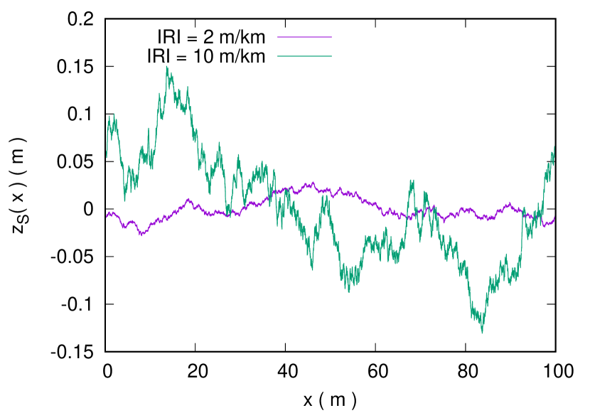
Figure 1: Vertical road surface displacement ($z_{S}$) as a function of horizontal displacement along the road surface ($x$), for two synthetic road surfaces at different International Roughness Indices, corresponding to a road surface of high quality ($IRI=2$ m/km, typical for “airport runways and superhighways” [4]) and another in poor repair ($IRI=10$ m/km, described in [4] as including “damaged pavements,” “maintained unpaved roads” and “rough unpaved roads” ). These data offer some sense of the level of disturbance in a road surface to be expected at different roughness indices.

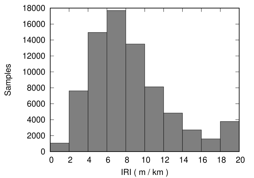
Figure 2: The distribution of the roughness index across secondary and tertiary roads in Ireland (after [16]). A “sample” is a 100 m section of road. The last bin includes samples with $IRI>20$ m/km. Clearly, cyclists on such roads must expected to encounter roughness indices up to about 15 m/km.

A second background consideration is the response of the human body to vibration. There are many contexts in which human bodies are exposed to potentially harmful vibration, and there is a correspondingly high level of research interest [5]. The rider of a bicycle is affected by the vibrations transmitted from the road, which may cause discomfort or, in extreme cases, injury. Exposure to vibration is conventionally quantified by the Vibration Dosage Value (VDV) [5, 19]. This is defined in terms of the acceleration $a(t)$ that the body is exposed to over some time interval $T$ as:

$$VDV = \left[\int_{0}^{T}a^{4}(t)dt\right]^{\frac{1}{4}}$$ (4)

$$\approx 1.4a_{\mathrm{rms}}T^{\frac{1}{4}},$$ (5)

where the value of the second expression is known as the Estimated Vibration Dosage Value (eVDV), and $a_{\mathrm{rms}}$ is the root mean square acceleration. (The fourth power of the acceleration in Equation 4, and the rather recherché units of $VDV$ that result, are motivated by a desire to emphasise the more extreme end of the spectrum of acceleration.) In many jurisdictions there are statutory limits controlling exposure to vibrations, which typically require $VDV\lesssim 20$ m s^-1.75. Separately, exposure to vibrations such that $a_{\mathrm{rms}}\gtrsim 10$ m s^-2 is prohibited, or at least deprecated. These criteria were not developed with cycling or any other athletic pursuits in mind, but rather with regard to repetitive exposure in daily life. Their relevance to occasional sporting activity might be doubted. Nevertheless, where they have been applied in a sporting context [6, 7, 8, 9, 10], they are usually found to be violated, sometimes grossly. Whether this is actually deleterious to cyclists appears unknown. As an instance of what cyclists may tolerate in practice, competitors in an approximately 30 km section of the Paris-Roubaix bicycle race are reported to have experienced $VDV>150$ m s^-1.75 and $a_{\mathrm{rms}}\gtrsim 25$ m s^-2 [7].

A topic directly relevant to the present work is the development of models for bodies exposed to vibration, and these are usually in a lumped element form involving masses, springs and damping elements (dashpots). Although more elaborate models are available [20], in this work, we have adopted a model with two degrees of freedom (described in section 3 below) in the interest of analytical tractability. The coefficients in the model relating to the human body are chosen with reference to the models described by [21], which refers to people seated without a backrest. The values of the parameters will be discussed below. Also of interest, however, is the amount of individual variation that may occur. The available studies essentially refer to representatives of the general population, and suggest variations around some mean of a few tens of percent [22]. One could suspect that practised cyclists might prove outliers in this distribution, but we have found no data bearing on this point.

3 Modelling

We first consider the model shown in Figure 3. This model imagines a cyclist with their weight carried on a saddle. The saddle is supported by the bicycle frame, which is itself supported by two tyres. The supporting effect of the bicycle frame and the tyres is represented by a stiffness constant $k_{B}$. We assume that the mass of the bicycle is negligible compared to the mass of the rider. The mass of the rider is divided between a lower body mass $m_{L}$ and an upper body mass $m_{U}$. These masses are connected by a spring with stiffness $k_{R}$ with an associated damping coefficient $c_{R}$, representing essentially the spine of the rider and dissipation associated with relative motions of the rider’s upper and lower body. We assume that damping in the bicycle and the tyres is negligible, as we are aware of no data to suggest otherwise. This model is mathematically identical to the “quarter car model” widely used in the automotive literature, but the meaning attached to the physical coefficients is different. Reference to the literature [21] enables us to associate reasonable values with these coefficients, viz, $m_{L}=33$ kg, $m_{U}=66$ kg, $k_{B}=200$ kN/m, $k_{R}=50$ kN/m and $c_{R}=1$ kN s/m. When a particular value is needed (in representative plots, for example), these values will be assumed unless there is a note to the contrary. We will see that $k_{B}$ is by far the most significant of these values, and fortunately this is a physical property of any given bicycle that is easy to measure. The other coefficients, of course, are not so easily measured and may be highly personal to particular riders. In analysing the model shown in Figure 3, we assume that linear stiffness coefficients are sufficient. We can distinguish (at least) two ways in which this assumption might fail. There are catastrophic possibilities: The bicycle could lose contact with the surface, or a wheel rim might strike the ground, for instance. These are rare in practice. A more significant incidence of nonlinearity is the tyre response, which is definitely not linear, in general [23]. However, small displacements around an equilibrium can almost always be modelled by a linear response, and we assume that this approximation can be applied.

Figure 3: A model for a bicycle crossing a rough surface, with no rotation of the bicycle about its centre of mass. The spring coefficient $k_{B}$ represents the combination of the bicycle frame and the tyres; $k_{R}$ is the stiffness of the riders torso (presumably mostly the spine); $m_{L}$ is the combined mass of the bicycle and the lower body of the rider (i.e. the legs and the pelvic region); $m_{U}$ is the remaining mass of the cyclist; and the damping coefficient $c_{R}$ is associated with the body of the rider. The values assigned to these coefficients are discussed in Section 3.

Inspection of Figure 3 shows that the basic equations are:

$$m_{L}\ddot{z}_{B}+c_{R}\left(\dot{z}_{B}-\dot{z}_{R}\right)-k_{R}(z_{R}-z_{B})+k_{B}z_{B} = k_{B}z_{S}(t)$$ (6)

$$m_{U}\ddot{z}_{R}+c_{R}\left(\dot{z}_{R}-\dot{z}_{B}\right)+k_{R}(z_{R}-z_{B}) = 0.$$ (7)

which are more conveniently written using $z_{C}=z_{R}-z_{B}$:

$$m_{L}\ddot{z}_{B}-c_{R}\dot{z}_{C}-k_{R}z_{C}+k_{B}z_{B} = k_{B}z_{S}(t)$$ (8)

$$\mu\ddot{z}_{C}+c_{R}\dot{z}_{C}+k_{R}z_{C}-\frac{k_{B}\mu}{m_{L}}z_{B} = -\frac{k_{B}\mu}{m_{L}}z_{S}(t).$$ (9)

where $\mu=m_{U}m_{L}/(m_{U}+m_{L})$. We assume all time variation is harmonic with angular frequency $\omega$, such that (for example) $z_{C}(t)=\tilde{z}_{C}\exp\left(-\omega t\right)$, where $\tilde{z}_{C}$ is an (in general) complex amplitude with complex conjugate denoted by $\tilde{z}^{*}_{C}$. Then we can show:

$$\frac{\tilde{z}_{C}}{\tilde{z}_{S}} = \frac{\omega^{2}\left(\frac{k_{B}}{m_{L}}\right)}{\omega^{4}+\frac{c_{R}}{\mu}i\omega^{3}-\left[\frac{k_{R}}{\mu}+\frac{k_{B}}{m_{L}}\right]\omega^{2}-\left(\frac{c_{R}k_{B}}{m_{U}m_{L}}\right)i\omega+\frac{k_{B}k_{R}}{m_{L}m_{U}}}.$$ (10)

Of concern is the power dissipated in the dashpot, which is given by

$$P_{\omega} = \frac{1}{2}c_{R}\omega^{2}\tilde{z}_{C}\tilde{z}_{C}^{*}$$ (11)

$$= \frac{1}{2}\frac{c_{R}\left(\frac{k_{B}}{m_{L}}\right)^{2}\omega^{6}\tilde{z}_{S}\tilde{z}^{*}_{S}}{\left[\omega^{4}-\left(\frac{k_{R}}{\mu}+\frac{k_{B}}{m_{L}}\right)\omega^{2}+\frac{k_{B}k_{R}}{m_{L}m_{U}}\right]^{2}+\left[\left(\frac{c_{R}}{\mu}\right)\omega^{3}-\frac{c_{R}k_{B}}{m_{U}m_{L}}\omega\right]^{2}}.$$ (12)

An example of this response is shown in Figure 4. This is (unsurprisingly) bimodal and shows that for these parameters (the ones discussed above), the maximum effect is at temporal frequencies of about 2-10 Hz and spatial wavelengths of 0.5-4 m. These spatial wavelengths of course depend on the speed of the bicycle which in this example is assumed to be 30 km/hr. Lower speeds will shift the response to shorter wavelengths, and vice versa. At normal cycling speeds, therefore, the response is caused by “roughness” and not “texture” in the sense of these terms discussed above.

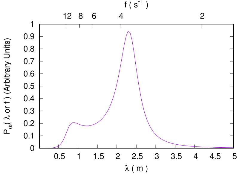
Figure 4: An example of the power dissipated in the model of Figure 3 as expressed by Equation 12 using the ordinary values of the parameters discussed in the text, and for a bicycle travelling at 30 km/hr. The upper axis shows temporal frequency and the lower axis spatial wavelength. Of course, the relationship between the axes depends on the speed. Cyclists may be surprised to see that the dominant effect is at such large wavelengths.

We now ask: What effect is produced when the disturbance $\tilde{z}_{S}$ is due to surface roughness characterised by Equation 2? If we consider a region around the wave number $n$ with infinitesimal size $dn$, then the effective amplitude of the disturbance in this region is [17]:

$$\tilde{z}_{S}\tilde{z}_{S}^{*}=2G_{d}(n)dn.$$ (13)

Then, noting that $\omega=2\pi nv$, for a bicycle travelling at speed $v$, and introducing the constant $\omega_{0}=\left(k_{B}c_{R}/m_{L}^{2}\right)^{\frac{1}{3}}$ and the dimensionless variable of integration $s=\omega/\omega_{0}$, we can write the wave number integrated power dissipation $P$ as

$$P = 2\pi vk_{B}n_{0}^{2}G_{d}(n_{0})I_{0}$$ (14)

where

$$I_{0} = \int_{0}^{\infty}\frac{s^{4}ds}{\left[s^{4}-\left(\frac{k_{R}}{\mu}+\frac{k_{B}}{m_{L}}\right)\frac{s^{2}}{\omega_{0}^{2}}+\frac{k_{B}k_{R}}{\omega_{0}^{4}m_{L}m_{U}}\right]^{2}+\left[\frac{c_{R}}{\mu\omega_{0}}s^{3}-\frac{c_{R}k_{B}}{m_{U}m_{L}\omega_{0}^{3}}s\right]^{2}}$$ (15)

$$= \frac{\pi}{2},$$ (16)

where $I_{0}$ is an instance of integral 3.112 of [24, p. 253], which can be evaluated using the formulae given therein. Hence:

$$P=\pi^{2}vk_{B}n_{0}^{2}G_{d}(n_{0})=F_{\mathrm{ro}}v.$$ (17)

Equation 1 follows from this result, combined with Equation 3. This outcome appears surprising, but similar results have been found in other dissipative systems excited by random processes [25, 26, 27, 28, 29, 30], some of them considerably more complex than the one under consideration here. The simplicity of the result, of course, depends on the assumption that Equation 2 is valid for all wave numbers. This cannot be exactly true. Even if the road surface is accurately described by Equation 2, the response of the bicycle must have a high frequency limit associated with the finite length of the tyre contact patch. However, Figure 4 shows that dominant part of the response is at wavelengths appreciably longer than the size of the contact patch, so this does not appear to be an important limitation of the present model.

The Vibrational Dose Value is dependent on the root mean square acceleration, which can be calculated in a similar way. By considering $\ddot{z}_{C}$, we can show that

$$a_{\mathrm{rms}}=\pi\sqrt{\frac{vG_{d}(n_{0})n_{0}^{2}k_{B}^{2}}{2m_{L}c_{R}}}.$$ (18)

Alternatively, making use of $\ddot{z}_{B}$ leads to:

$$a_{\mathrm{rms}}=\pi\sqrt{\frac{vG_{d}(n_{0})n_{0}^{2}}{2}\left[\frac{c_{R}k_{B}}{m_{U}^{2}}+\frac{\left(m_{U}k_{B}-m_{L}k_{R}\right)^{2}}{c_{R}m_{U}^{2}m_{L}}+\frac{k_{R}^{2}}{c_{R}m_{U}}\right]}.$$ (19)

Either of these can be used in conjunction with Equation 5 to estimate the Vibration Dose Value, but only Equation 19 conforms with the prescribed standard method for VDV calculation [19], which requires $a_{\mathrm{rms}}$ to be evaluated at the point of entry into the body (the saddle, in this case, so the acceleration at $z_{B}$). The standard also requires the use of a frequency filter [19, 31]. However, the frequency filter has insignificant effect over the range suggested by Figure 4. Perhaps more practically important than these details is the difficulty of precisely defining the values of the parameters.

Figure 5: A model for a bicycle that is able to rotate about its centre of mass as it passes across the surface.

We consider now a model with two wheels, shown in Figure 5. (This incidentally is not the same as the “half car model” often used for road vehicles.) We assume that both wheels follow the same path across the road surface, so that the disturbances at each wheel differ only by a time delay, $\Delta t$. The motion in this case is a superposition of translations of the centre of mass and rotations about the centre of mass. Relative to the model discussed above, the extra effect that is introduced is the possibility that the vehicle can tilt as the wheels pass over the road surface. The nature of this effect varies with the wavelength of disturbances in the road surface. If the wheelbase is an integral multiple of the wavelength, there is no effect, because both wheels rise and fall in phase with each other. If, however, the wheelbase is a half integral multiple of the wavelength, and the centre of mass is midway between the wheels, the motion is a pure rotation around the centre of mass, and there is no vertical displacement of the centre of mass. One might therefore guess that the effect will be to reduce the resistance by a factor of two, and this is not far from the truth, as the detailed argument shows.

Consider a frame of reference in which the bicycle is stationary. In this frame of reference, the rear wheel contacts the ground at $x_{WB}$ and the front wheel at $x_{WF}$ so that the wheel base $L_{W}=x_{WF}-x_{WB}$. The bicycle has a centre of mass at $x_{M}$, and naturally $x_{WB}\leq x_{M}\leq x_{WF}$. Road surface roughness causes vertical displacements at each wheel, and these displacements are denoted by $z_{WB}$ and $z_{WF}$. By convention, these quantities are taken to be zero when the bicycle is at rest on a flat surface. When $z_{WB}$ and $z_{WF}$ are not zero, the centre of mass will be displaced vertically by an amount $z_{M}$ and a rotation about the centre of mass by an angle $\theta$ will occur, so that:

$$z_{M} = \left(1-\xi_{M}\right)z_{WB}+\xi_{M}z_{WF}$$ (20)

$$\theta = \frac{z_{WF}-z_{WB}}{L_{W}}$$ (21)

where $\xi_{M}=x_{M}/L_{W}$ and we assume $\sin\theta\approx\theta$. The passage of the bicycle over the road surface produces a displacement of the surface at $z_{WB}$ given by $z_{S}(t)$ and at $z_{WF}$ given by $z_{S}(t+\Delta t)$, where the time constant $\Delta t$ is $L_{W}/v$ when the bicycle travels at speed $v$. A force constant is associated with each of these displacments, such that the vertical force at the center of mass is

$$F_{M} = F_{WB}+F_{WF}$$ (22)

$$= -k_{WB}\left[z_{WB}-z_{S}(t)\right]-k_{WF}\left[z_{WF}-z_{S}(t+t_{0})\right]$$ (24)

$$= -\left(k_{WB}+k_{WF}\right)z_{M}+L_{W}\left[\xi_{M}k_{WB}-(1-\xi_{M})k_{WF}\right]\theta$$

$$+k_{WB}z_{S}(t)+k_{WF}z_{s}(t+\Delta t)$$

and the torque around the centre of mass is

$$T_{M} = L_{W}\left[\left(1-\xi_{M}\right)F_{WF}-\xi_{M}F_{WB}\right]$$ (26)

$$= -\left\{L_{W}\left[(1-\xi_{M})k_{WF}-\xi_{M}k_{WB}\right]z_{M}+L_{W}^{2}\xi_{M}\left[\xi_{c}k_{WB}+(1-\xi_{M})k_{WF}\right]\theta\right\}$$

$$-L_{W}\left[\xi_{M}k_{WB}z_{S}(t)-(1-\xi_{M})k_{WF}z_{S}(t+t_{0})\right].$$

We ensure that the bicycle is horizontal at equilibrium by assuming

$$k_{WB} = \left(1-\xi_{M}\right)k_{B}$$ (27)

$$k_{WF} = \xi_{M}k_{B}$$ (28)

so that

$$F_{M} = -k_{B}z_{c}+k_{B}\left[(1-\xi_{M})z_{S}(t)+\xi_{M}z_{S}(t+\Delta t)\right]$$ (29)

$$T_{M} = -2k_{B}L_{W}^{2}\xi_{M}^{2}(1-\xi_{M})\theta-k_{B}L_{W}(1-\xi_{M})\xi_{M}\left[z_{S}(t)-z_{S}(t+\Delta t)\right].$$ (30)

Equations 27 and 28 uncouple the vertical displacement from the angular displacement. Moreover, in the approximation $\cos\theta\approx 1$ (for small angular displacements), movements of the masses parallel to the $x$ axis can be neglected. Hence we can identify $z_{M}$ with $z_{B}$ of the previous model, and write the equations of motion for the displacements along the $z$ axis as (c.f. Equations 6-7):

$$m_{L}\ddot{z}_{B}+c_{R}\dot{z}_{C}-k_{R}z_{C}+k_{B}z_{B} = k_{B}\left[(1-\xi_{M})z_{S}(t)+\xi_{M}z_{S}(t+\Delta t)\right]$$ (31)

$$m_{U}\ddot{z}_{R}+c_{R}\dot{z}_{C}+k_{R}z_{C} = 0,$$ (32)

and we see that the effect of introducing the rocking motion is only to modify the forcing term. In the frequency domain, the time delay $\Delta t$ becomes a phase difference

$$\phi=\frac{2\pi L_{W}}{\lambda}=\frac{\omega L_{W}}{v}$$ (33)

where $\lambda$ is a spatial wavelength and $v$ is the speed of the bicycle. Consequently, the effect of introducing the rocking motion is to modify the driving term in the model, such that:

$${{\tilde{z^{\prime}}}_{S}}^{2}=\left[\left(1-\xi_{M}\right)^{2}+2\left(1-\xi_{M}\right)\xi_{M}\cos\phi+\xi_{M}^{2}\right]\tilde{z}_{S}^{2}.$$ (34)

So the required change is to insert the rocking factor

$$R_{\omega}=\frac{{{\tilde{z^{\prime}}}_{S}}^{2}}{\tilde{z}_{S}^{2}}=\left(1-\xi_{M}\right)^{2}+2\left(1-\xi_{M}\right)\xi_{M}\cos\phi+\xi_{M}^{2}.$$ (35)

into the integral in Equation 15. Unfortunately we have found no exact treatment of the integral that arises when the rocking factor is included. The value of this integral is a function of the speed $v$ of the bicycle because of the phase factor given by Equation 33. Values of the rocking factor as a function of speed are shown in Figure 6, where the integral has been computed by a quadrature. The oscillations arise because the cosinusoidal term in Equation 35 is convoluted with a response such as the one shown in Figure 4. Evidently, this leads to the remarkable situation that the roughness resistance and possibly the total resistance are not always monotonically increasing functions of speed. This effect can be more extreme for parameters different from the base values discussed above. For example, reducing the damping coefficient can lead to more pronounced oscillations. This might conceivably be an exploitable effect in situations where a bicycle travels at nearly constant speed for long intervals, such as in a time trial on level ground. However, more generally this seems likely to be an exotic curiosity. For the purposes of further discussion, we assume that for a typical cyclist travelling at variable speed, the oscillatory effects average out and so we approximate the rocking factor as

$$R\approx\left(1-\xi_{M}\right)^{2}+\xi_{M}^{2}.$$ (36)

A typical value of $\xi_{M}$ is about 0.4 [32], so that $R\approx 0.52$. This correction applied to Equation 17 is the roughness resistance that we will employ in further discussion. Similarly, the rocking factor can be inserted into Equation 18 or 19 to estimate the Vibration Dose Value.

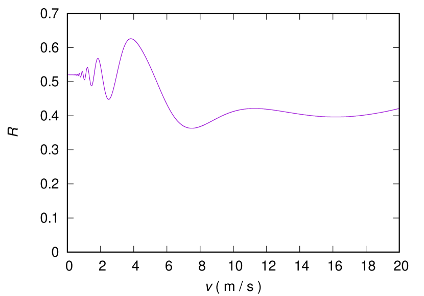
Figure 6: The rocking factor $R$ found by integrating Equation 35 over the model response. In detail this curve depends on all of the model parameters. This example was computed using the parameters discussed in the text.

4 Discussion

Understanding the significance of the results obtained above requires that we link the roughness resistance with parameters of transparent practical significance, and consider the relationship of the roughness resistance, the rolling resistance and the aerodynamic drag. Rolling resistance is not, in general, quantitatively well understood [1], meaning there is no theory available to calculate the rolling resistance from first principles. There are, however, extensive measurements of the coefficient of rolling resistance $c_{\mathrm{rr}}$ (see, e.g., [33]). The most important parameters are the tyre inflation pressure $P$ and the tyre radius $R_{T0}$. A convenient form is

$$c_{\mathrm{rr}}=c_{\mathrm{rr}}^{(0)}\left[\frac{P^{(0)}R^{(0)}_{T0}}{PR_{T0}}\right]^{\frac{1}{2}},$$ (37)

where the coefficient $c_{\mathrm{rr}}^{(0)}$ is inferred from experiments, while $P^{(0)}$ and $R^{(0)}_{T0}$ are reference values.

We have seen that the stiffness of the bicycle ($k_{B}$) is one of the most important factors affecting the roughness resistance, and this stiffness is strongly influenced by the tyre stiffness, $k_{T}$. Hence it is important to have a quantitative understanding of the relationship between the physical parameters characterising a bicycle tyre, and the stiffness of the same tyre. A convenient model is described in [23], in which the bicycle wheel and tyre is characterised by the tyre radius under no load, $R_{T0}$, the rim width, $W_{L}$, the wheel radius, $R_{W}$, and the inflation pressure, $P$. (Where a numerical value is required later, we assume $W_{L}=2R_{T0}$.) This model shows that if the tyre deflection from the no load condition is $d$, then the force exerted is

$$F_{T}\approx\alpha\beta Pd^{\frac{3}{2}},$$ (38)

where $\alpha=1.259$ is a dimensionless numerical constant and $\beta$ is a geometrical factor involving complex sub-formulae that we will not quote. If the tyre bears a load $M_{L}$ then the equilibrium deflection is

$$d=\left(\frac{M_{L}g}{\alpha\beta P}\right)^{\frac{2}{3}}.$$ (39)

We assume that normal cycling is characterised by small changes in deflection near this equilibrium point, so that the linear force constant is

$$k_{T}=\left.\frac{dF_{T}}{dz}\right|_{z=d}=\frac{3}{2}\left(\alpha\beta P\right)^{\frac{2}{3}}\left(M_{L}g\right)^{\frac{1}{3}}.$$ (40)

We will be interested in establishing the smallest force constant that can be achieved. For fixed geometrical parameters, this requires choosing the smallest permissible tyre pressure. Standards developed by the European Tyre and Rim Technical Organisation allow a 30% maximum tyre deflection at equilibrium load [34, p. M9], relative to the unloaded tyre height $2R_{T0}$ and this condition implies a minimum tyre pressure given by

$$P_{\mathrm{min}}=\frac{M_{L}g}{\alpha\beta\left(0.6R_{T0}\right)^{\frac{3}{2}}}.$$ (41)

and so the minimum force constant is

$$k_{T,\mathrm{min}}=\frac{M_{L}g}{0.6R_{T0}},$$ (42)

surprisingly independent of the rim width $W_{L}$, although the minimum pressure is not. There is also a maximum spring constant, associated with the maximum type pressure. What determines this? The tension in a tyre casing of thickness $h$ is [23]:

$$\sigma=\frac{R_{T0}P}{h}.$$ (43)

For a given tyre casing construction (with $h$ fixed, and some $\sigma_{\mathrm{max}}$, above which the tyre will fail), there is therefore a maximum inflation pressure inversely proportional to the radius, such that $R_{T0}P_{\mathrm{max}}$ is constant. Under this constraint, the rolling resistance when $P=P_{\mathrm{max}}$ is independent of $R_{T0}$. That this holds exactly here is contingent on the particular forms of Equation 37 and the tyre model. However, for any reasonable alternatives to these, the result will hold at least approximately.

These preliminaries enable us to address the practical implications of Equation 17. Let us first consider a traditional high performance bicycle, with a stiff frame ($k_{F}=1$ MN/m) and narrow tyres ($2R_{T0}=23$ mm). The rolling resistance parameters in Equation 37 are chosen using data from [33] to be representative of contemporary high performance tyres. The curve in the upper panel of Figure 7 labelled $R_{T0}=1.15$ cm and $P=P_{\mathrm{max}}$ shows the resistance force encountered by this bicycle as a function of the roughness index. An initial point is that the presence of roughness significantly increases the total resistance on practically any road. Even at the upper limit of well maintained roads ($IRI=5$ m/km), the resistance is more than doubled, and at $IRI=10$ m/km, the resistance is six times larger. This implies that roughness resistance is a matter of concern for almost all cyclists, whether (for examples) engaged in competition on well-maintained roads, or audax events during which poorer surfaces predominate. What can be done to minimise the roughness effect? Clearly, because of Equation 17, only one recourse is available, and that is to reduce the stiffness of the bicycle. In general, and supposing $k_{T}$ is specified for one tyre:

$$k_{B}\approx\frac{2k_{T}k_{F}}{2k_{T}+k_{F}}.$$ (44)

So one can reduce $k_{B}$ by reducing either $k_{F}$ or $k_{T}$ or both. Let us consider these options separately, and address tyre stiffness first. Equation 40 shows that the simplest measure, which is always available, is to reduce the tyre pressure. If this is insufficient, then the tyre radius can be increased as well, and the minimum stiffness available is then given by Equation 42. Equation 42 suggests that the stiffness can be reduced without bound by increasing $R_{T0}$, but this course of action obviously has practical limits. As an example, we consider $2R_{T0}=40$ mm, but the choice here does not affect the conclusions that will be drawn. Also plotted in Figure 7 are the resistance forces for this larger tyre for three pressure cases: $P_{\mathrm{max}}$, $P_{\mathrm{min}}$ and the pressure $P_{\mathrm{opt}}$ that minimises the total resistance. On smoother roads ($IRI\lesssim 5$ m/km), the optimal choice is $P_{\mathrm{opt}}=P_{\mathrm{max}}$ and in this regime the total resistance is indistinguishable from the narrower tyre considered above. On rougher roads ($IRI\gtrsim 10$ m/km) the optimal choice is $P_{\mathrm{opt}}=P_{\mathrm{min}}$ and here the total resistance is much less than the narrower tyre, by a factor of between 1.5 and 2 in the range shown. In the transitional regime $5\lesssim IRI\lesssim 10$ m/km, there is a corresponding transition in the optimal pressure, which is shown in the lower panel of Figure 7. These data show that the wider tyre has an optimal resistance that is never higher than the narrower tyre, but significantly lower when $IRI\gtrsim 5$ m/km. The difficulty here, of course, is that cyclists cannot usually predict in advance what range of roughness index they will encounter, and nor (in most cases) can they rapidly adapt their tyre pressure to changing road conditions. Let us now turn to the other possibility, namely reducing the frame stiffness $k_{F}$. Reports in the cycling press suggest that the stiffness of frames has fallen in recent years. Typical now seems to be $100\lesssim k_{F}\lesssim 300$ kN/m, with some instances of $k_{F}\lesssim 100$ kN/m. Figure 8 shows the same calculations as Figure 7 with the exception that $k_{F}=200$ kN/m. Clearly, the regime in which the narrower and wider tyres are indistinguishable has extended to $IRI\lesssim 10$ m/km and the rough regime is postponed to $IRI\gtrsim 15$ m/km. Of course, frames with even lower $k_{F}$ (which exist) will move these regimes to even larger $IRI$. Consequently, reduced frame stiffness achieves much the same outcome in respect of resistance as reduced tyre stiffness, but without the practical complication of varying the tyre pressure, because the optimal pressure for all but the most extreme road conditions is $P_{\mathrm{max}}$. The clear implication is that a highly compliant (i.e. low stiffness) frame is the most practical way of reducing the resistance experienced on rough roads.

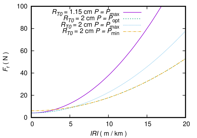
(a)

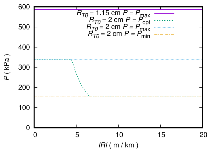
(b)

Figure 7: (a) The total resistance force $F_{\mathrm{r}}=F_{\mathrm{rr}}+F_{\mathrm{ro}}$ as a function of the roughness index for bicycles with stiff frames ($k_{F}=1$ MN/m). Data are shown for a traditional high performance tyre with $2R_{T0}=23$ mm inflated to the maximum permissible pressure, and for a modern “all road” tyre ($2R_{T0}=40$ mm) with three different pressure choices: The maximum allowed ($P_{\mathrm{max}}$), the minimum allowed ($P_{\mathrm{min}}$), and the pressure that minimizes the resistance force at a given value of $IRI$ ($P_{\mathrm{opt}}$). (b) The tyre pressures corresponding to the data shown in (a), showing that the optimal solution is $P_{\mathrm{max}}$ for $IRI\lesssim 5$ m/km, $P_{\mathrm{min}}$ for $IRI\gtrsim 10$ m/km, with a transitional regime in between. (Recall that 100 kPa $\approx$ 1 Bar $\approx~{}15$ psi.)

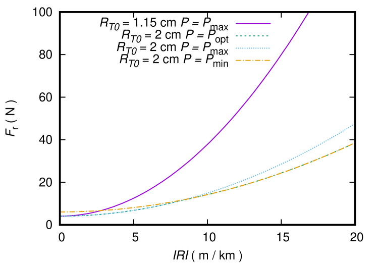
(a)

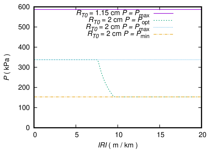
(b)

Figure 8: (a) As in Figure 7, with the difference that the second bicycle with $2R_{T0}=40$ mm has a frame that is appreciably less stiff, with $k_{F}=200$ kN/m rather than $k_{F}=1$ MN/m. Evidently, this change substantially reduces the resistance force. (b) As in Figure 7, showing that the transition between the high and low pressure optimal solutions is postponed to $IRI>10$ m/km by reducing the frame stiffness.

Aerodynamic drag [35, 36, 1] is generally proportional to $v^{2}$ and is characterised by the drag area $C_{D}A$, where $C_{D}$ is a dimensionless drag coefficient and $A$ is a relevant area. This is usually a larger force than the resistance we have been examining, and it is affected by the choice of tyre size, because larger tyres increase the aerodynamic drag. Typically the drag area for a cyclist varies from around 0.2 m² to 0.4 m² [35, 36]. For the purpose of this discussion, we select the middling value $C_{D}A=0.3$ m². With reference to wind tunnel data [37], we assume that a tyre wider than the lowest value we have considered ($2R_{T0}=23$ mm) adds to the drag area at a rate of 0.015 m² per cm of additional tyre diameter, which means that when $2R_{T0}=4$ cm, the drag area is increased by about 10 %. We evaluate the effect of this additional drag by solving a power balance equation:

$$P_{C}=\frac{1}{2}\rho C_{D}Av^{3}+\left(c_{\mathrm{rr}}Mg+F_{\mathrm{ro}}\right)v^{2},$$ (45)

where $P_{C}$ is the power available from the cyclist and $\rho$ is the density of air (assumed to be 1.2 kg m^-3). The results of this calculation are shown in Figure 9, which compares the traditional high performance bicycle discussed above ($2R_{T0}=23$ mm and $k_{F}=1$ MN/m) with an otherwise similar machine with $2R_{T0}=4$ cm and $k_{F}=200$ kN/m (as in Figure 8). These data show that for $IRI\lesssim 5$ m/km, the additional aerodynamic drag caused by the larger tyre is appreciable. In competitions such as time trials, the speed difference shown here would be important. In Figure 10, we consider the case of a bicycle frame with exceptionally low stiffness, $k_{F}=50$ kN/m. In this case, the bicycle stiffness given by Equation 44 is dominated by the frame stiffness, and tyre stiffness is barely a factor. Consequently, the additional aerodynamic drag of a larger tyre is a disadvantage at all values of IRI. But this is unlikely to be the only consideration in practice. Attempting to ride a narrow tyre on a surface with $IRI>10$ m/km could be a highly unsatisfactory experience, that could well mitigate in favour of a larger tyre despite the apparent aerodynamic limitations. In addition, the question of what degree of stiffness is desirable in a bicycle is complex: There are considerations other than minimising roughness resistance.

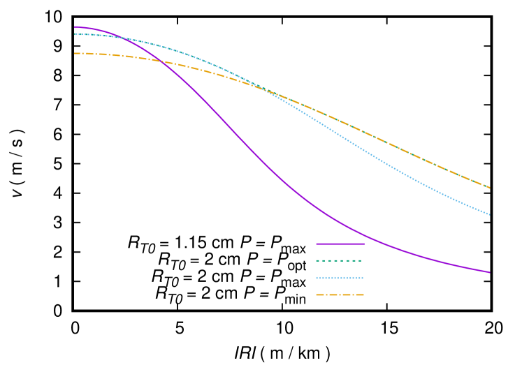
(a)

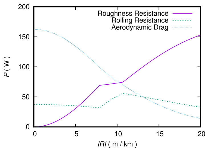
(b)

Figure 9: (a) Bicycle speeds obtained by solving the power balance Equation 45 including aerodynamic drag, roughness resistance, and rolling resistance, for a cyclist with $P_{C}=200$ W. The bicycles are the same as in Figure 8, but the bicycle with larger tyres is assumed to have increased drag area as discussed in the text. This additional drag reduces speed for insufficient compensation when $IRI\lesssim 5$ m/km. On roads with $IRI\gtrsim 5$, roughness resistance is more important and the drag area less so. Reduced frame stiffness is also important, as in Figure 8. (b) The total power divided between roughness resistance, rolling resistance and aero dynamic drag for total power $P_{C}=200W$, for the case in (a) with $2R_{T0}=4$ cm, $P=P_{\mathrm{opt}}$ and $k_{F}=200$ kN/m.

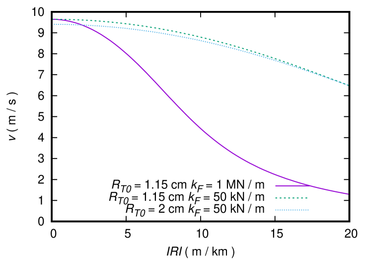
Figure 10: These data are similar to Figure 9, but compare bicycles with different frame stiffness. In particular, considered here is the case where $k_{F}=50$ kN/m, approximately the lowest value that seems presently practical. In all these cases $P=P_{\mathrm{max}}$. Under these conditions, the bicycle stiffness is dominated by the frame stiffness (see Equation 44), and tyre stiffness has almost no influence.

Figure 11 shows the root mean square acceleration calculated from Equation 18 for the conditions of Figure 9. In conjunction with Equation 5 these data suggest what others have surmised [6, 8, 7, 9, 10], that cycling activities are likely to breach the thresholds for VDV exposure. The data in Figure 11 tie this conclusion rather more specifically to road roughness and bicycle characteristics than previous work but the outcome is much the same. For instance, if $VDV=20$ m s^-1.75 is the threshold (a typical statutory limit), this will be breached in 1 minute of cycling with $a_{\mathrm{rms}}=10$ m s^-2. If we accepted $VDV=150$ m s^-1.75 (as occurred in the Paris-Roubaix race), then the threshold will be breached in about 4 hours. However, whether thresholds set for protection from occupational exposure over a working life can be appropriately applied to intense sporting activities undertaken sporadically is far from obvious, and is presumably likely to be the subject of further research. Whether cycling as a means of daily transport causes dangerous VDV exposure seems also unknown.

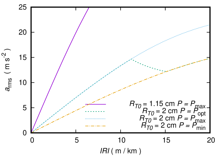
(a)

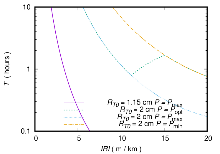
(b)

Figure 11: (a) The root means square acceleration for the same cases shown in Figure 9, calculated using Equation 19. These data show that the pressure that minimises the resistance force (as in Figure 8) is not always identical with the pressure that minimises $a_{\mathrm{rms}}$. (b) The permissible riding time if the Vibration Dosage Value is to remain below $150$ m s^-1.75, using the data in (a) above in conjunction with Equation 5.

5 Concluding remarks

Previous works have established that what is here called roughness resistance is an important effect, but they have not offered any systematic understanding or quantification. This paper shows that this effect can be described by surprisingly simple expressions that depend only on two clearly defined and easily measured physical parameters, namely the vertical stiffness of the bicycle and the International Roughness Index of the surface on which the bicycle travels (Equation 17). The stiffness of the bicycle can be approximately decomposed into a frame stiffness and a tyre stiffness (Equation 44). Either of these can be dominant. In traditional high performance bicycles, the tyre stiffness is much less than the frame stiffness; for a typical modern bicycle, both are important; and for certain modern bicycles with exceptionally low frame stiffness, the frame stiffness is the dominant factor. There are immediate implications for the optimal choice of tyre diameter, because increasing the tyre diameter reduces the tyre stiffness and consequently the roughness resistance. However, increasing the tyre diameter also increases the aerodynamic drag area. Which of these effects is the most important depends on the objectives of the cyclist and on the circumstances (in particular, on the road roughness). There is no generally optimal solution.

The cycling public may find these considerations recondite. However, practically all cyclists are exposed to vibration due to road roughness. As we have seen, there is reason to be concerned about this. Equations 5 and 18 can be used to connect road condition surveys with the Vibration Dose Value experienced by cyclists in general, in a manner that may be of interest to authorities concerned with both pavement maintenance and public health.

Disclosure statement

No potential conflict of interest was reported by the author.

References

- [1] Wilson DG, Schmidt T. Bicycling Science. 4th ed. Cambridge, MA, USA: MIT Press; 2020.
- [2] Heine J. The All-Road Bike Revolution. Seattle, Washington: Bicycle Quarterly Press; 2020. Available from: https://www.renehersecycles.com/shop/print/books/the-all-road-bike-revolution/.
- [3] Poertner J. Part 4B: Rolling Resistance and Impedance ; 2019. Available from: https://blog.silca.cc/part-4b-rolling-resistance-and-impedance.
- [4] Sayers MW, Gillespie TD, Paterson WDO. Guidelines for Conducting and Calibrating Road Roughness Measurements. World Bank Technical Paper. 1986;ISBN: 9780821305904 Number: Technical Paper 46; Available from: https://trid.trb.org/view.aspx?id=278294.
- [5] Griffin MJ. Handbook of Human Vibration. Revised edition ed. Amersterdam: Academic Press; 1996.
- [6] Tarabini M, Saggin B, Scaccabarozzi D. Whole-body vibration exposure in sport: four relevant cases. Ergonomics. 2015 Jul;58(7):1143–1150. Publisher: Taylor & Francis _eprint: https://doi.org/10.1080/00140139.2014.961969; Available from: https://doi.org/10.1080/00140139.2014.961969.
- [7] Duc S, Puel F, Bertucci W. Vibration exposure on cobbles sectors during Paris Roubaix. In: Journal of Science and Cycling; Vol. 5; Jul.; Caen, France; 2016. p. 19–20. Available from: https://hal.univ-reims.fr/hal-03124457.
- [8] Roseiro LM, Neto MA, Amaro AM, et al. Hand-arm and whole-body vibrations induced in cross motorcycle and bicycle drivers. International Journal of Industrial Ergonomics. 2016 Nov;56:150–160. Available from: https://www.sciencedirect.com/science/article/pii/S0169814116302153.
- [9] Doria A, Marconi E, Munoz L, et al. An experimental-numerical method for the prediction of on-road comfort of city bicycles. Vehicle System Dynamics. 2021 Sep;59(9):1376–1396. Publisher: Taylor & Francis _eprint: https://doi.org/10.1080/00423114.2020.1759810; Available from: https://doi.org/10.1080/00423114.2020.1759810.
- [10] Edwards PI, Holsgrove TP. Thunder road - whole-body vibration during road cycling, and the effect of different seatpost designs to minimise it. Journal of Sports Sciences. 2021 Mar;39(5):489–495. Publisher: Routledge _eprint: https://doi.org/10.1080/02640414.2020.1829361; Available from: https://doi.org/10.1080/02640414.2020.1829361.
- [11] International Organization for Standardization. ISO 8608:2016 ; 2016. Available from: https://www.iso.org/cms/render/live/en/sites/isoorg/contents/data/standard/07/12/71202.html.
- [12] Zang K, Shen J, Huang H, et al. Assessing and Mapping of Road Surface Roughness based on GPS and Accelerometer Sensors on Bicycle-Mounted Smartphones. Sensors (Basel, Switzerland). 2018 Mar;18(3):914. Available from: https://www.ncbi.nlm.nih.gov/pmc/articles/PMC5876687/.
- [13] Ahmed HU, Hu L, Yang X, et al. Effects of smartphone sensor variability in road roughness evaluation. International Journal of Pavement Engineering. 2021 Sep;0(0):1–6. Publisher: Taylor & Francis _eprint: https://doi.org/10.1080/10298436.2021.1946059; Available from: https://doi.org/10.1080/10298436.2021.1946059.
- [14] Cafiso S, Di Graziano A, Marchetta V, et al. Urban road pavements monitoring and assessment using bike and e-scooter as probe vehicles. Case Studies in Construction Materials. 2022 Jun;16:e00889. Available from: https://www.sciencedirect.com/science/article/pii/S2214509522000213.
- [15] Kropáč O, Múčka P. Indicators of Longitudinal Road Unevenness and their Mutual Relationships. Road Materials and Pavement Design. 2007 Jan;8(3):523–549. Publisher: Taylor & Francis _eprint: https://doi.org/10.1080/14680629.2007.9690087; Available from: https://doi.org/10.1080/14680629.2007.9690087.
- [16] Feighan K. Pavement Condition Study Report. Ireland: Department of Environment, Heritage and Local Government; 2004.
- [17] Agostinacchio M, Ciampa D, Olita S. The vibrations induced by surface irregularities in road pavements – a Matlab® approach. European Transport Research Review. 2014 Sep;6(3):267–275. Number: 3 Publisher: SpringerOpen; Available from: https://etrr.springeropen.com/articles/10.1007/s12544-013-0127-8.
- [18] Department for Transport. Road Traffic Estimates in Great Britain, 2022: Traffic in Great Britain by Vehicle Type ; 2022. Available from: https://www.gov.uk/government/statistics/road-traffic-estimates-in-great-britain-2022/road-traffic-estimates-in-great-britain-2022-traffic-in-great-britain-by-vehicle-type.
- [19] ISO. Human response to vibration — Measuring instrumentation — Part 1: General purpose vibration meters. Geneva, Switzerland: International Organization for Standardization; 2017. ISO 8041-1:2017. Available from: https://www.iso.org/standard/70648.html.
- [20] Liang CC, Chiang CF. A study on biodynamic models of seated human subjects exposed to vertical vibration. International Journal of Industrial Ergonomics. 2006 Oct;36(10):869–890. Available from: https://www.sciencedirect.com/science/article/pii/S0169814106001296.
- [21] Muksian R, Nash CD. On frequency-dependent damping coefficients in lumped-parameter models of human beings. Journal of Biomechanics. 1976 Jan;9(5):339–342. Available from: https://www.sciencedirect.com/science/article/pii/0021929076900555.
- [22] Toward MGR, Griffin MJ. Apparent mass of the human body in the vertical direction: Inter-subject variability. Journal of Sound and Vibration. 2011 Feb;330(4):827–841. Available from: https://www.sciencedirect.com/science/article/pii/S0022460X10005821.
- [23] Renart J, Roura-Grabulosa P. Deformation of an inflated bicycle tire when loaded. American Journal of Physics. 2019 Feb;87(2):102–109. Publisher: American Association of Physics Teachers; Available from: http://aapt.scitation.org/doi/full/10.1119/1.5086008.
- [24] Gradshteyn IS, Ryzhik IM. Table of Integrals, Series, and Products. 7th ed. Amsterdam ; Boston: Academic Press; 2007.
- [25] Clough RW, Penzien J. Dynamics of Structures. McGraw-Hill; 1993.
- [26] Pippard AB. The Physics of Vibration. Cambridge: Cambridge University Press; 1989. Available from: https://www.cambridge.org/core/books/physics-of-vibration/FFA074D42B188D50C888FE8E8545A47E.
- [27] Langley RS. Can an undamped oscillator dissipate energy? Journal of Sound and Vibration. 1997 Oct;206(4):624–626. Available from: https://www.sciencedirect.com/science/article/pii/S0022460X9791066X.
- [28] Smith MC, Swift SJ. Power dissipation in automotive suspensions. Vehicle System Dynamics. 2011 Feb;49(1-2):59–74. Publisher: Taylor & Francis _eprint: https://doi.org/10.1080/00423110903427421; Available from: https://doi.org/10.1080/00423110903427421.
- [29] Clark J, Smith MC. Power absorption invariance for brownian spring forcing. In: 2012 IEEE 51st IEEE Conference on Decision and Control (CDC); Dec.; 2012. p. 4396–4399. ISSN: 0743-1546.
- [30] Langley RS. A general mass law for broadband energy harvesting. Journal of Sound and Vibration. 2014 Feb;333(3):927–936. Available from: https://www.sciencedirect.com/science/article/pii/S0022460X13007906.
- [31] Gonçalves JPC, Ambrósio JAC. Optimization of Vehicle Suspension Systems for Improved Comfort of Road Vehicles Using Flexible Multibody Dynamics. Nonlinear Dynamics. 2003 Oct;34(1):113–131. Available from: https://doi.org/10.1023/B:NODY.0000014555.46533.82.
- [32] Yizhaq H, Baran G. A new method for computing the centre of mass of a bicycle and rider. Physics Education. 2010 Sep;45(5):500. Available from: https://dx.doi.org/10.1088/0031-9120/45/5/007.
- [33] Biermann J. Bicycle Rolling Resistance | Rolling Resistance Tests ; 2023. Available from: https://www.bicyclerollingresistance.com/.
- [34] European Tyre and Rim Technical Organisation. Standards Manual. Brussels, Belgium: ETRTO; 2003.
- [35] Crouch TN, Burton D, LaBry ZA, et al. Riding against the wind: a review of competition cycling aerodynamics. Sports Engineering. 2017 Jun;20(2):81–110. Available from: https://doi.org/10.1007/s12283-017-0234-1.
- [36] Malizia F, Blocken B. Bicycle aerodynamics: History, state-of-the-art and future perspectives. Journal of Wind Engineering and Industrial Aerodynamics. 2020 May;200:104134. Available from: https://www.sciencedirect.com/science/article/pii/S0167610520300441.
- [37] Crane R, Morton C. Drag and Side Force Analysis on Bicycle Wheel–Tire Combinations. Journal of Fluids Engineering. 2018 Mar;140(061205). Available from: https://doi.org/10.1115/1.4039513.