Proof-of-concept: Using ChatGPT to Translate and Modernize an Earth System Model from Fortran to Python/JAX

Abstract

Earth system models (ESMs) are vital for understanding past, present, and future climate, but they suffer from legacy technical infrastructure. ESMs are primarily implemented in Fortran, a language that poses a high barrier of entry for early career scientists and lacks a GPU runtime, which has become essential for continued advancement as GPU power increases and CPU scaling slows. Fortran also lacks differentiability — the capacity to differentiate through numerical code — which enables hybrid models that integrate machine learning methods. Converting an ESM from Fortran to Python/JAX could resolve these issues. This work presents a semi-automated method for translating individual model components from Fortran to Python/JAX using a large language model (GPT-4). By translating the photosynthesis model from the Community Earth System Model (CESM), we demonstrate that the Python/JAX version results in up to 100x faster runtimes using GPU parallelization, and enables parameter estimation via automatic differentiation. The Python code is also easy to read and run and could be used by instructors in the classroom. This work illustrates a path towards the ultimate goal of making climate models fast, inclusive, and differentiable.

1 Introduction

Over the last decades, climate models have evolved from very coarse ocean-atmosphere models to complex Earth system models including all Earth components — the ocean, atmosphere, cryosphere and land and detailed biogeochemical cycle — [12] and are now being used to address a vast array of questions from projecting natural sinks [14] to the impact of land use change on climate [13]. Over decades of model development, Earth system models have become huge computing programs written in Fortran or C, for legacy and compatibility reasons. Yet most early career scientists do not know those languages, which hinders model development.

Further, because of their complexity, running these models is resource-intensive [35; 31]. Most (perhaps all) models rely on parallelized CPU hardware, even though highly-parallelized code can now be run more efficiently on Graphics Processing Units (GPUs) [1] or Tensor Processing Units (TPUs) [9]. Earth system modeling would dramatically benefit from hardware acceleration, so that models could be run at higher resolutions and resolve important fine-scale processes like ocean eddies or deep convection. Using high-level languages also makes model code robust to future hardware evolution; this type of (r)evolution is already starting in other fields of physics [7; 3].

Finally, Earth System Models are starting to use machine learning (ML) to represent subgrid processes [32; 15; 40; 4]. Because of their native Python infrastructure, those machine learning components are not straightforward to implement in Fortran- or C/C++-based Earth System Models and require a bridge (e.g., Fortran to Python), without the flexibility to do online learning (updating between ML and the physical code while the physical model runs) [30] [8]. The missing piece is automatic differentiation, which allows us to take the partial derivatives to any parameters in the code. Python has many libraries supporting differentiation; one of these is JAX, which enables automatic differentiation and hardware acceleration of Python code while maintaining a near-Python visual look [6].

In this work, we intend to break this Earth System Model language and hardware deadlock by modernizing Earth System Model codes to run on modern hardware (e.g., GPUs) and enabling automatic differentiation [25] using Python and JAX to enhance both efficiency and precision [6], while also making model development more inclusive. To realize this goal, our approach leverages recent developments in large-language models (LLMs) to rapidly translate code from one language to another [19] [38]. Specifically, we split the model into units using static analysis, develop a topological sort order based on dependencies, and translate each unit using OpenAI’s GPT-4 [34].

Our contribution is twofold: we demonstrate the Python/JAX version’s utility through an example model (leaf-level photosynthesis in the Community Land Model (CLM) of CESM), and we offer open source tools to address translation challenges. As an added benefit, we also demonstrate that the Python translation can be computationally more efficient than the original model by leveraging GPUs with the JAX library.

2 Translation Workflow

Large language models alone cannot translate a whole codebase for two reasons. First, there are more tokens (i.e., words) in a typical codebase than a model like GPT-4 can accept in its token limit. Second, the model alone often writes incorrect code. To resolve these issues, we’ve implemented a divide-and-conquer approach that splits a Fortran codebase into ordered units using static analysis, generates Python/JAX translations using the GPT-4 API, and uses unit test outputs to iterate on the generated code. Figure 1 shows the architecture of our translation process (see details in appendix).

Figure 1: Workflow for translating a climate model from Fortran to Python, using static analysis, code generation, and unit testing.

3 Translation Evaluation

3.1 Runtime

We made several versions of the original photosynthesis code, which were mostly LLM-generated. There are four Python versions: NumPy makes a direct translation of the algorithm from Fortran into NumPy. Numba takes NumPy and adds just-in-time (jit) compiling using Numba [21]. SciPy uses a SciPy library function for rootfinding [37], and JAX uses the JAX library for jit compilation. Note that this JAX version, in contrast to the other Python versions, required substantial modification from the LLM-generated code. See Figure 2 for a visual comparison.

The code we translated takes as input an initial value of internal partial pressure of CO2 in the leaf, and iteratively solves for the x-intercept of a function for stomatal conductance based on this guess [27] [22]. To generate these runtime results, we ran each of the versions (4 Python versions + 1 on GPU, 1 Fortran version) using vectors sampling from a range of input values from 35 to 70 Pa.

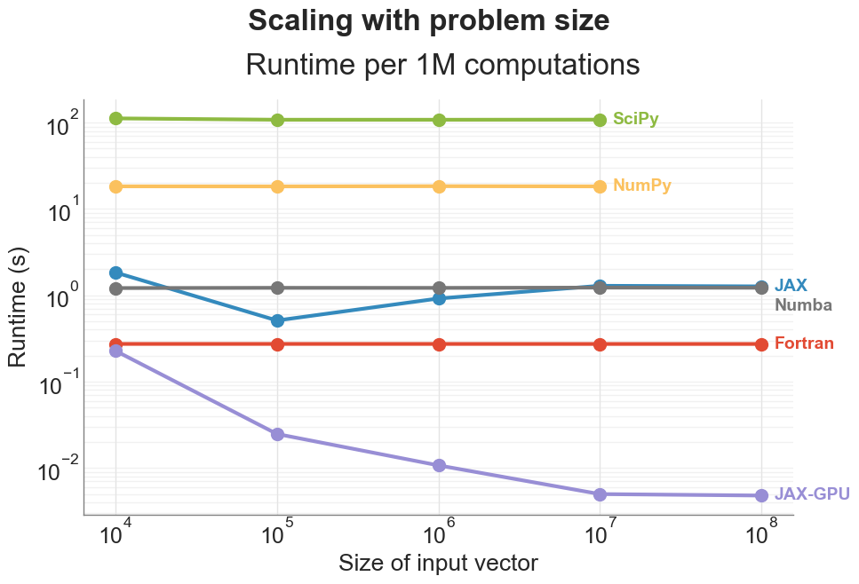
Figure 2: Comparing runtime of leaf-level photosynthesis in several Python translations with the original Fortran version. Runtime was measured on an Amazon EC2 G5.4xlarge instance with one NVIDIA A10G GPU.

From the runtime results (smaller is better), we observe that JAX-GPU was the fastest, with Fortran a full two orders of magnitude slower. JAX on CPU and Numba (both jit-compiled) are slightly slower than Fortran. NumPy and SciPy are both even slower. From this we can conclude two things. First, these results show that GPU parallelization on a GPU can lead to significant runtime improvements relative to sequential Fortran on a roughly equivalent CPU (included with the same machine). Second, even JAX-CPU and Numba perform reasonably well compared to Fortran, suggesting that jit-compilation alone can make up for much of the speed difference between Fortran and Python.

3.2 Parameter Estimation

While the equations describing photosynthesis are well understood, there are many uncertain parameters that vary by plant species or even leaf position in the canopy. To demonstrate the usefulness of automatic differentiation in Python, we chose one parameter to estimate: the maximum rate of carboxylation, Vcmax, which plays a key role in determining the co-limited rate of assimilation.

One method to obtain the optimal set of parameters, is by running a strategically sampled parameter perturbation experiment, where multiple parameters are varied simultaneously to identify the best set of parameters (e.g., [39]; [18]; [10]). However, studies have shown that it is challenging to find global optimal parameter settings that improve overall skill in a climate model (e.g., [26]; [11]). An alternative method, inspired by machine learning, is using gradient descent to find parameter values that align the model with measured data [33]. Gradient descent has become an increasingly optimized operation in Python, thanks to techniques like minibatches and stochastic methods [5].

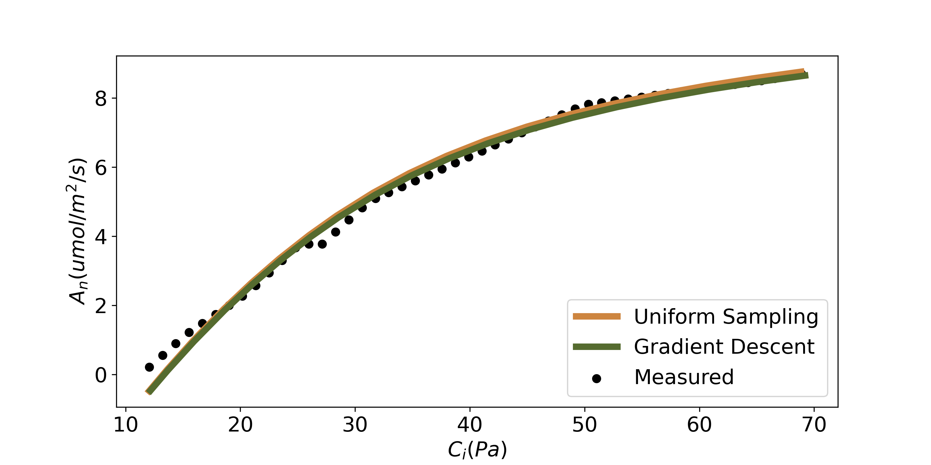
Figure 3: Measured (points) and modeled (lines) relationship between the internal partial pressure of CO2 (Pa) and the rate of assimilation (umol/m2/s). The modeled values use the Vcmax parameter value selected using either uniform sampling (orange) or gradient descent (green).

In Figure 3, we compared parameter estimation methods for optimizing the Vcmax parameter using observed measurements of assimilation rate (An) at a range of partial pressures of CO2 within leaf (observations from a Ponderosa pine tree at the US-Me2 AmeriFlux site in Central Oregon). We employed a uniform sampling parameter perturbation scheme and gradient descent to identify the Vcmax setting that minimized the error between the model simulations and observations. In this simplified leaf-level model, uniform sampling and gradient descent converged to similar values (Vcmax=38.776 $\mu$mol $\text{CO}_{\text{2}}\text{ m}^{-2}\text{s}^{-1}$ and Vcmax=38.383 $\mu$mol $\text{CO}_{\text{2}}\text{ m}^{-2}\text{s}^{-1}$ respectively), though gradient descent took fewer iterations (10 gradient descent steps as opposed to 50 sample points in uniform sampling) and achieves a lower loss value (7.26 and 6.39 respectively in mean squared error).

These results support the idea that gradient descent and automatic differentiation would also be more efficient when estimating more parameters for multiple modules of CLM. Our code conversion to JAX unleashes the use of ML-methods, such as stochastic gradient descent, for efficient parameter tuning through automatic differentiation [2].

3.3 Future Work

While implementing automatic translation, we faced challenges including poor Fortran generation quality, inaccurate unit tests, incorrect use of imported modules, and GPT-4 token limits. For scaling up translation, next steps could include using data flow and compiler representations for translation (as in [36] and [16]), building logging to track function calls, and designing copilot-style interfaces to support human translators. Solving these engineering challenges will further decrease the amount of manual work involved in translating and modernizing climate models.

4 Conclusions

Migrating a full climate model from Fortran to Python, even with language models like ChatGPT, is challenging due to important dependencies and logical errors in code generation. However, translating individual components (like leaf-level photosynthesis) from Fortran to Python/JAX is both useful and now within reach, and tools like the static analysis and language models presented in this work will make this easier. Even with just a single component translated and modernized in Python, one could experiment with parameter estimation, measuring sensitivity to parameters (quantifying parametric uncertainty and getting faster feedback loops for model development), running on GPU, and translating model components for offline experiments.

Eventually, this work aims to pave the way for the development of a future where climate models are differentiable and GPU/TPU-friendly, making them faster and more accurate, while also written in high-level languages so that they are more inclusive of junior scientists to accelerate progress on the critical program of climate change modeling and adaptation.

5 Appendix

This appendix provides details on the implementation of the translation method, useful for those who seek to build on this work. Our semi-automated translation process works in two steps: first we divide the Fortran codebase into manageable chunks using static analysis. Second, we "conquer" (translate) each of these chunks from Fortran to Python by running unit tests with iterative language model generations.

5.1 Prompting

With large language models (LLMs), changing the prompt can significantly affect the generated response [24]. Therefore, we developed a variety of prompts for the tasks of translating Fortran to Python, writing Fortran unit tests, and writing Python unit tests. The GPT-4 Chat Completion API accepts prompts in the form of chat messages [29]. In this work, we used the System message and one User message for each API call, as shown in Table 1. Some sample outputs are shown in Table 2.

Task	System Prompt	User Prompt
Generate Fortran unit tests	You’re a proficient Fortran programmer.	Given Fortran code, write unit tests using funit. Example: FORTRAN CODE: [...] FORTRAN TESTS: [...] Your turn: FORTRAN CODE: {fortran_code} FORTRAN TESTS:
Translate Fortran to Python	You’re a programmer proficient in Fortran and Python.	Convert the following Fortran function to Python. ‘‘‘{python_code}‘‘‘
Translate Fortran unit tests to Python	You’re a programmer proficient in Fortran and Python.	Convert the following unit tests from Fortran to Python using pytest. No need to import the module under test. ‘‘‘{unit_tests}‘‘‘
Generate Python unit tests	You’re a programmer proficient in Python and unit testing. You can write and execute Python code by enclosing it in triple backticks, e.g. “‘code goes here“‘	Generate 5 unit tests for the following Python function using pytest. No need to import the module under test. ‘‘‘{python_function}‘‘‘
Iteratively improve code	You’re a programmer proficient in Fortran and Python. You can write and execute Python code by enclosing it in triple backticks, e.g. ‘‘‘code goes here‘‘‘. When prompted to fix source code and unit tests, always return a response of the form: SOURCE CODE: ‘‘‘<python source code>‘‘‘ UNIT TESTS: ‘‘‘<python unit tests>‘‘‘. Do not return any additional context.	Function being tested: {python_function} Here are some unit tests for the above code and the corresponding output. Unit tests: {python_unit_tests} Output from ‘pytest‘: ‘‘‘ {python_test_results} ‘‘‘ Modify the source code to pass the failing unit tests. Return a response of the following form: SOURCE CODE: ‘‘‘<python source code>‘‘‘ UNIT TESTS: ‘‘‘<python unit tests>‘‘‘

Table 1: Prompts used for each task. Braces ({}) represent interpolated variables from the current translation task. Sections marked […] were omitted for brevity.

5.2 Divide

The goal of this step is to divide the large initial codebase into small problems, which can be solved by the ‘conquer‘ module in order. We have two important constraints here: the sub-problems have to be small enough that they fit within the LLM’s context length, and they have to be individually testable.

If we want the code chunks to be short enough for a model’s context length, we should translate one function at a time (the whole module would be too large for ChatGPT). We also note that the functions must be translated in a particular order, because of their dependencies. For example, consider the functions represented by Figure 4. In this case, we can’t use the ‘hybrid‘ function until we’ve translated the other eight functions.

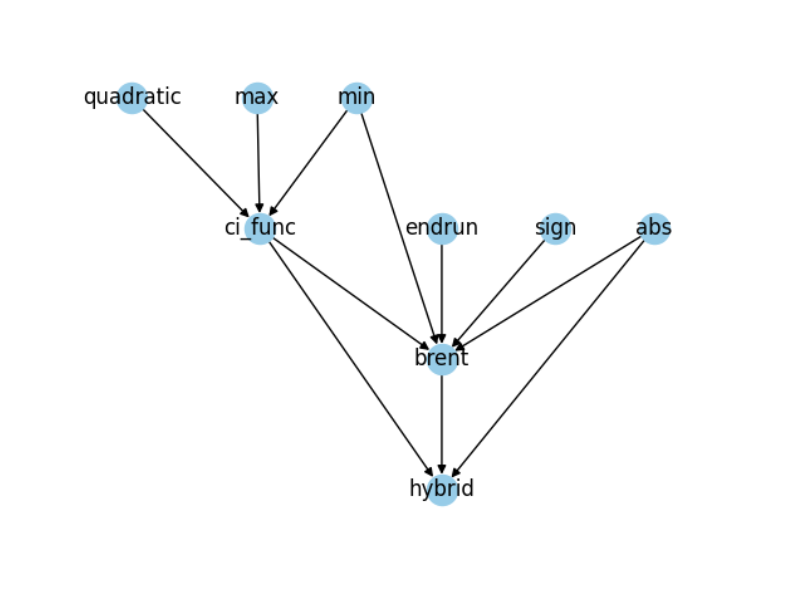
Figure 4: Dependency graph for the function ‘hybrid‘ from the leaf-level photosynthesis module. Each node corresponds to a function defined in this module, and each edge corresponds to a function call.

Since we have here a directed acyclic graph (DAG) [23], a topological sorting algorithm would yield a correct order for translating the functions one-by-one. This is exactly the approach we take for dividing the problem: generate a dependency graph of symbols, and then use topological sorting to determine an order of translation. For each unit of code, we then generate and run unit tests using GPT-4 using prompts from Table 1.

5.2.1 Generating a dependency graph

To create a dependency graph, we take a two-step approach. First, we divide the codebase into testable units (functions, types, or subroutines) and find the other units referenced by each unit. Then, we form a dependency graph based on these references. These steps are marked as step 1 and 2 in Figure 5.

To chunk the code into units and find references, one method is using a parsing tool such as fparser to return a syntax tree from the original source code. However, these tools only work on single files and can’t unambiguously locate function definitions, requiring manual searches. So a parser is effective for chunking code but not for finding references.

To find references, there are at least two options. First, one could use the language server protocol (LSP), used in text editors like VSCode for features like "Go to Definition" [28] [17]. Second, one could prompt a language model, providing an index of all names in the project as context . This second approach has its limitations, because the index may exceed context length and generations may be unreliable. Given these downsides, LSP seems to be a good balanced approach for parsing dependencies, given its proven reliability and efficiency with codebases of any size. In this work, we created Python scripts using both LSP and fparser to compute dependency graphs. However, for even better results, using a compiler’s data flow or control flow for ordered translation could be an exciting future direction.

Our ultimate approach is documented in Figure 5.

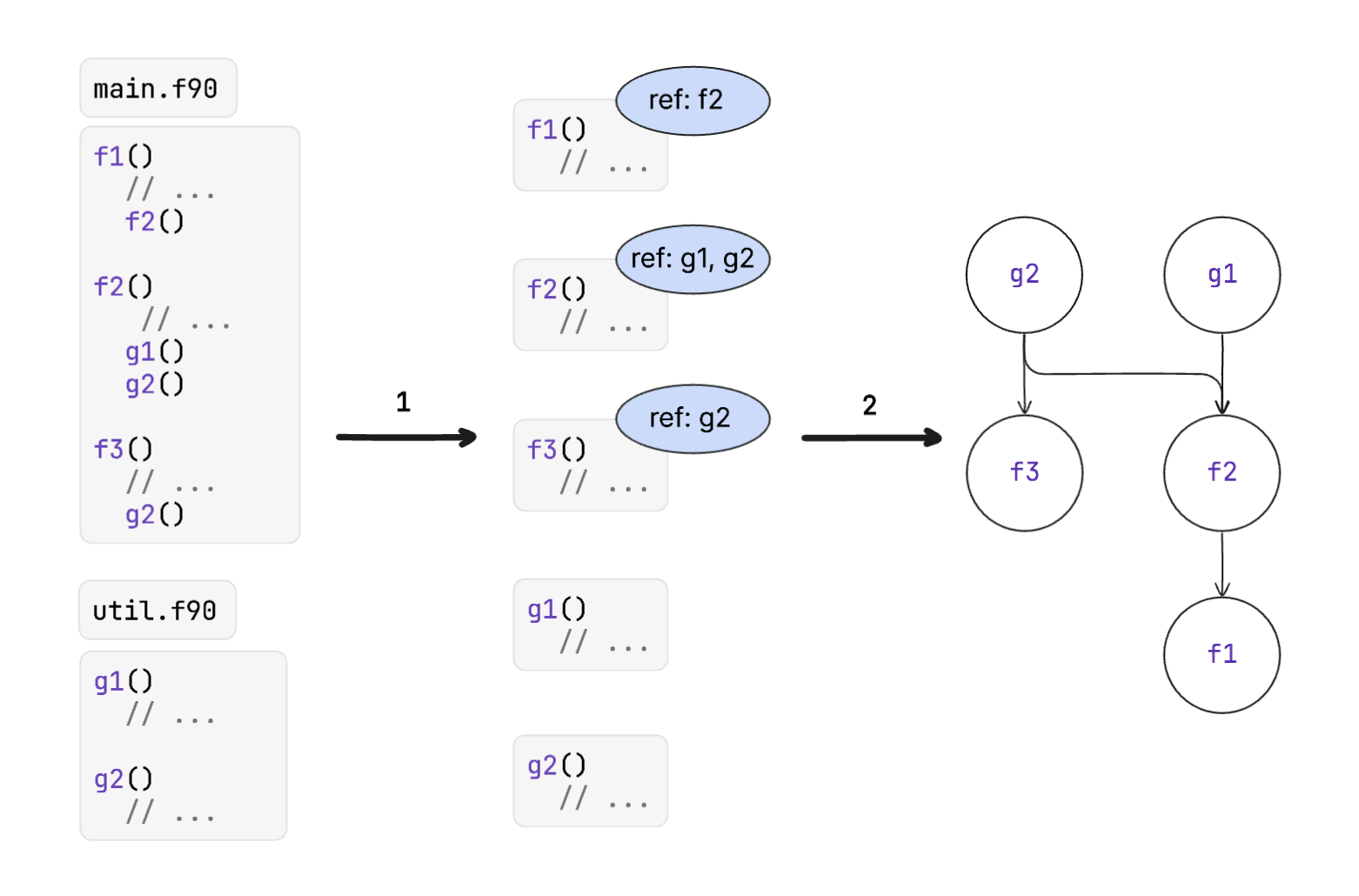
Figure 5: Visualization of code chunking process. In step 1, we chunk a codebase into individual units using a parsing tool and trace references. In step 2, we use those references to form a dependency graph.

5.2.2 Developing unit tests

Once we use dependency graphs to create units, each of these units needs to be unit tested. In other words, we should be able to run a chunk of the Fortran code, along with the corresponding Python translation, and get the same outputs for a given set of inputs. To do this, we propose (as future work) implementing a logging tool, which would log the inputs and outputs for a Fortran function when it runs within the original code. A tool like kgen would be good for this [20]. Then we could use these inputs and outputs to generate unit tests. For now, we rely on GPT-4 to generate unit tests using its own knowledge, using the prompts from Table 1.

5.3 Conquer

Assuming the divide step works well, we would want a consistent way to make GPT-4 write code that passes our unit tests. To do this, we have implemented an iterative approach to code generation, which takes in a chunk of Fortran code, along with corresponding unit tests, and generates corresponding Python code and Python unit tests. Then we make a Docker image that runs the tests automatically. If any tests cases fail, the test output gets passed back into the GPT-4 API, and it returns some revised code. This approach is depicted in Figure 1.

5.4 Combining divide and conquer

In summary, we created a module for identifying the dependencies between symbols in Fortran source code, as well as a command-line interface for generating and iteratively updating a Python translation. To provide a proof of concept, here are some demonstrations of runtime and parameter estimation for the leaf-level photosynthesis module from the Community Land Model, leveraging the power of automatic differentiation for model parameter tuning.

Fortran Source Code	Fortran Unit Tests
⬇ elemental real(r8) function daylength(lat, decl) ! … some comments omitted for conciseness use shr_infnan_mod, only : nan => shr_infnan_nan, & assignment(=) use shr_const_mod , only : SHR_CONST_PI ! !ARGUMENTS: real(r8), intent(in) :: lat real(r8), intent(in) :: decl ! !LOCAL VARIABLES: real(r8) :: my_lat real(r8) :: temp ! number of seconds per radian of hour-angle real(r8), parameter :: secs_per_radian = 13750.9871_r8 ! epsilon for defining latitudes "near" the pole real(r8), parameter :: lat_epsilon = 10._r8 * epsilon(1._r8) ! Define an offset pole as slightly less than pi/2 to avoid ! problems with cos(lat) being negative real(r8), parameter :: pole = SHR_CONST_PI/2.0_r8 real(r8), parameter :: offset_pole = pole - lat_epsilon ! lat must be less than pi/2 within a small tolerance if (abs(lat) >= (pole + lat_epsilon)) then daylength = nan ! decl must be strictly less than pi/2 else if (abs(decl) >= pole) then daylength = nan ! normal case else ! Ensure that latitude isn’t too close to pole, to avoid ! problems with cos(lat) being negative my_lat = min(offset_pole, max(-1._r8 * offset_pole, lat)) temp = -(sin(my_lat)*sin(decl))/(cos(my_lat) * cos(decl)) temp = min(1._r8,max(-1._r8,temp)) daylength = 2.0_r8 * secs_per_radian * acos(temp) end if end function daylength	⬇ module test_daylength ! Tests of the daylength function in DaylengthMod use funit use shr_kind_mod , only : r8 => shr_kind_r8 use shr_const_mod, only : SHR_CONST_PI use DaylengthMod , only : daylength implicit none save real(r8), parameter :: tol = 1.e-3_r8 contains @Test subroutine test_standard_points() ! Tests multiple points, not edge cases @assertEqual([26125.331_r8, 33030.159_r8], daylength([-1.4_r8, -1.3_r8], 0.1_r8), tolerance=tol) end subroutine test_standard_points @Test subroutine test_near_poles() ! Tests points near the north and south pole, which ! should result in full night and full day @assertEqual([0.0_r8, 86400.0_r8], daylength([-1.5_r8, 1.5_r8], 0.1_r8), tolerance=tol) end subroutine test_near_poles @Test subroutine test_edge_cases() ! Tests the edge cases, not the valid cases @assertEqual([1.e100_r8, -1.e100_r8], daylength([1.5_r8, -1.5_r8], 0.1_r8), tolerance=tol) end subroutine test_edge_cases end module test_daylength
Python Source Code	Python Unit Tests
⬇ import numpy as np def daylength(lat, decl): """ ␣␣␣␣Calculate␣the␣length␣of␣the␣day␣(in␣hours)␣given␣the ␣␣␣␣latitude␣and␣the␣declination␣of␣the␣sun.␣␣This␣is ␣␣␣␣the␣number␣of␣seconds␣between␣sunrise␣and␣sunset. ␣␣␣␣Returns␣NaN␣if␣input␣arguments␣are␣invalid. ␣␣␣␣…␣[more␣comments␣omitted␣for␣conciseness] ␣␣␣␣""" # Number of seconds per radian of hour-angle secs_per_radian = 13750.9871 # Epsilon for defining latitudes "near" the pole lat_epsilon = 10.0 * np.finfo(float).eps pole = np.pi / 2 offset_pole = pole - lat_epsilon # Lat must be less than pi/2 within a small tolerance # Decl must be strictly less than pi/2 lat = np.where(abs(lat) >= pole + lat_epsilon, np.NAN, lat) decl = np.where(abs(decl) >= pole, np.NAN, decl) my_lat = np.clip(lat, -offset_pole, offset_pole) temp = -np.tan(my_lat) * np.tan(decl) temp = np.clip(temp, -1, 1) return 2.0 * secs_per_radian * np.arccos(temp) class Bounds: def __init__(self, begg, endg): self.begg = begg self.endg = endg def compute_max_daylength(bounds, lat, obliquity): """Compute␣max␣daylength␣for␣each␣grid␣cell""" max_daylength = [] for g in range(bounds.begg, bounds.endg): max_decl = obliquity if lat[g] < 0.0: max_decl = -max_decl max_daylength.append(daylength(lat[g], max_decl)) return max_daylength	⬇ import numpy as np import pytest from daylength import daylength # tolerance tol = 1e-3 def test_standard_points(): assert np.allclose(daylength(np.array([-1.4, -1.3]), 0.1), np.array([26125.331, 33030.159]), atol=tol) def test_near_poles(): assert np.allclose(daylength(np.array([-1.5, 1.5]), 0.1), np.array([0.0, 86400.0]), atol=tol) def test_north_pole(): assert abs(daylength(np.pi/2.0, 0.1) - 86400.0) < tol assert abs(daylength(np.pi/1.999, 0.1) - 86400.0) < tol def test_south_pole(): assert abs(daylength(-1.0 * np.pi/2.0, 0.1)) < tol assert abs(daylength(-1.0 * np.pi/1.999, 0.1)) < tol def test_error_in_decl(): assert np.isnan(daylength(-1.0, -3.0)) def test_error_in_lat_scalar(): assert np.isnan(daylength(3.0, 0.1)) def test_error_in_lat_array(): my_result = daylength(np.array([1.0, 3.0]), 0.1) assert np.isfinite(my_result[0]) assert np.isnan(my_result[1])

Table 2: Sample outputs from a translation run on the day length function in the Community Land Model. Clockwise from top-left: original Fortran code, original Fortran unit tests, generated Python code, and generated Python unit tests.

References

- Baji [2018] Toru Baji. Evolution of the gpu device widely used in ai and massive parallel processing. In 2018 IEEE 2nd Electron devices technology and manufacturing conference (EDTM), pages 7–9. IEEE, 2018.
- Baydin et al. [2018] Atilim Gunes Baydin, Barak A Pearlmutter, Alexey Andreyevich Radul, and Jeffrey Mark Siskind. Automatic differentiation in machine learning: a survey. Journal of Marchine Learning Research, 18:1–43, 2018.
- Bezgin et al. [2023] Deniz A Bezgin, Aaron B Buhendwa, and Nikolaus A Adams. Jax-fluids: A fully-differentiable high-order computational fluid dynamics solver for compressible two-phase flows. Computer Physics Communications, 282:108527, 2023.
- Bolton and Zanna [2019] Thomas Bolton and Laure Zanna. Applications of deep learning to ocean data inference and subgrid parameterization. Journal of Advances in Modeling Earth Systems, 11(1):376–399, 2019.
- Bottou [2012] Léon Bottou. Stochastic gradient descent tricks. In Neural Networks: Tricks of the Trade: Second Edition, pages 421–436. Springer, 2012.
- Bradbury et al. [2018] James Bradbury, Roy Frostig, Peter Hawkins, Matthew James Johnson, Chris Leary, Dougal Maclaurin, George Necula, Adam Paszke, Jake VanderPlas, Skye Wanderman-Milne, and Qiao Zhang. Jax: composable transformations of python+numpy programs, 2018. URL http://github.com/google/jax.
- Campagne et al. [2023] Jean-Eric Campagne, François Lanusse, Joe Zuntz, Alexandre Boucaud, Santiago Casas, Minas Karamanis, David Kirkby, Denise Lanzieri, Yin Li, and Austin Peel. Jax-cosmo: An end-to-end differentiable and gpu accelerated cosmology library. arXiv preprint arXiv:2302.05163, 2023.
- Carliner [2004] Saul Carliner. An overview of online learning. 2004.
- Cass [2019] Stephen Cass. Taking ai to the edge: Google’s tpu now comes in a maker-friendly package. IEEE Spectrum, 56(5):16–17, 2019.
- Couvreux et al. [2021] Fleur Couvreux, Frédéric Hourdin, Daniel Williamson, Romain Roehrig, Victoria Volodina, Najda Villefranque, Catherine Rio, Olivier Audouin, James Salter, Eric Bazile, Florent Brient, Florence Favot, Rachel Honnert, Marie-Pierre Lefebvre, Jean-Baptiste Madeleine, Quentin Rodier, and Wenzhe Xu. Process-based climate model development harnessing machine learning: I. a calibration tool for parameterization improvement. Journal of Advances in Modeling Earth Systems, 13(3):e2020MS002217, 2021. doi: https://doi.org/10.1029/2020MS002217. URL https://agupubs.onlinelibrary.wiley.com/doi/abs/10.1029/2020MS002217.
- Dagon et al. [2020] K. Dagon, B. M. Sanderson, R. A. Fisher, and D. M. Lawrence. A machine learning approach to emulation and biophysical parameter estimation with the community land model, version 5. Advances in Statistical Climatology, Meteorology and Oceanography, 6(2):223–244, 2020. doi: 10.5194/ascmo-6-223-2020. URL https://ascmo.copernicus.org/articles/6/223/2020/.
- Edwards [2011] Paul N Edwards. History of climate modeling. Wiley Interdisciplinary Reviews: Climate Change, 2(1):128–139, 2011.
- Findell et al. [2017] Kirsten L Findell, Alexis Berg, Pierre Gentine, John P Krasting, Benjamin R Lintner, Sergey Malyshev, Joseph A Santanello Jr, and Elena Shevliakova. The impact of anthropogenic land use and land cover change on regional climate extremes. Nature communications, 8(1):989, 2017.
- Friedlingstein et al. [2014] Pierre Friedlingstein, Malte Meinshausen, Vivek K Arora, Chris D Jones, Alessandro Anav, Spencer K Liddicoat, and Reto Knutti. Uncertainties in cmip5 climate projections due to carbon cycle feedbacks. Journal of Climate, 27(2):511–526, 2014.
- Gentine et al. [2018] Pierre Gentine, Mike Pritchard, Stephan Rasp, Gael Reinaudi, and Galen Yacalis. Could machine learning break the convection parameterization deadlock? Geophysical Research Letters, 45(11):5742–5751, 2018.
- Guo et al. [2020] Daya Guo, Shuo Ren, Shuai Lu, Zhangyin Feng, Duyu Tang, Shujie Liu, Long Zhou, Nan Duan, Alexey Svyatkovskiy, Shengyu Fu, Michele Tufano, Shao Kun Deng, Colin B. Clement, Dawn Drain, Neel Sundaresan, Jian Yin, Daxin Jiang, and Ming Zhou. Graphcodebert: Pre-training code representations with data flow. CoRR, abs/2009.08366, 2020. URL https://arxiv.org/abs/2009.08366.
- Hansen and Nikiteas [2022] Chris Hansen and Ioannis Nikiteas. fortls, 2022. URL https://github.com/fortran-lang/fortls.
- Hourdin et al. [2017] Frédéric Hourdin, Thorsten Mauritsen, Andrew Gettelman, Jean-Christophe Golaz, Venkatramani Balaji, Qingyun Duan, Doris Folini, Duoying Ji, Daniel Klocke, Yun Qian, Florian Rauser, Catherine Rio, Lorenzo Tomassini, Masahiro Watanabe, and Daniel Williamson. The art and science of climate model tuning. Bulletin of the American Meteorological Society, 98(3):589–602, 2017. doi: https://doi.org/10.1175/BAMS-D-15-00135.1. URL https://journals.ametsoc.org/view/journals/bams/98/3/bams-d-15-00135.1.xml.
- Kasneci et al. [2023] Enkelejda Kasneci, Kathrin Seßler, Stefan Küchemann, Maria Bannert, Daryna Dementieva, Frank Fischer, Urs Gasser, Georg Groh, Stephan Günnemann, Eyke Hüllermeier, et al. Chatgpt for good? on opportunities and challenges of large language models for education. Learning and individual differences, 103:102274, 2023.
- Kim and Dennis [2019] Youngsung Kim and John Dennis. Kgen: Fortran kernel generator, 2019. URL https://github.com/NCAR/KGen.
- Lam et al. [2015] Siu Kwan Lam, Antoine Pitrou, and Stanley Seibert. Numba: A llvm-based python jit compiler. In Proceedings of the Second Workshop on the LLVM Compiler Infrastructure in HPC, pages 1–6, 2015.
- Lawrence [2023] D. et al. Lawrence. Clm50 technical note. 2023. URL http://www.cesm.ucar.edu/models/cesm2/land/CLM50_Tech_Note.pdf.
- Lipsky and Greenland [2022] Ari M Lipsky and Sander Greenland. Causal directed acyclic graphs. JAMA, 327(11):1083–1084, 2022.
- Liu et al. [2021] Pengfei Liu, Weizhe Yuan, Jinlan Fu, Zhengbao Jiang, Hiroaki Hayashi, and Graham Neubig. Pre-train, prompt, and predict: A systematic survey of prompting methods in natural language processing. CoRR, abs/2107.13586, 2021. URL https://arxiv.org/abs/2107.13586.
- Margossian [2019] Charles C Margossian. A review of automatic differentiation and its efficient implementation. Wiley interdisciplinary reviews: data mining and knowledge discovery, 9(4):e1305, 2019.
- McNeall et al. [2016] D. McNeall, J. Williams, B. Booth, R. Betts, P. Challenor, A. Wiltshire, and D. Sexton. The impact of structural error on parameter constraint in a climate model. Earth System Dynamics, 7(4):917–935, 2016. doi: 10.5194/esd-7-917-2016. URL https://esd.copernicus.org/articles/7/917/2016/.
- Medlyn et al. [2011] Belinda E Medlyn, Remko A Duursma, Derek Eamus, David S Ellsworth, I Colin Prentice, Craig VM Barton, Kristine Y Crous, Paolo De Angelis, Michael Freeman, and Lisa Wingate. Reconciling the optimal and empirical approaches to modelling stomatal conductance. Global Change Biology, 17(6):2134–2144, 2011.
- Microsoft [2020] Microsoft. Language server protocol, 2020. URL https://github.com/microsoft/language-server-protocol.
- OpenAI [2023] OpenAI. Gpt - openai api, 2023. URL https://platform.openai.com/docs/guides/gpt/chat-completions-api. Accessed: 2023-06-15.
- Ott et al. [2020] Jordan Ott, Mike Pritchard, Natalie Best, Erik Linstead, Milan Curcic, and Pierre Baldi. A fortran-keras deep learning bridge for scientific computing. Scientific Programming, 2020:1–13, 2020.
- Palmer [2014] Tim Palmer. Climate forecasting: Build high-resolution global climate models. Nature, 515(7527):338–339, 2014.
- Rasp et al. [2018] Stephan Rasp, Michael S Pritchard, and Pierre Gentine. Deep learning to represent subgrid processes in climate models. Proceedings of the National Academy of Sciences, 115(39):9684–9689, 2018.
- Ruder [2016] Sebastian Ruder. An overview of gradient descent optimization algorithms. arXiv preprint arXiv:1609.04747, 2016.
- Sanderson [2023] Katharine Sanderson. Gpt-4 is here: what scientists think. Nature, 615(7954):773, 2023.
- Schär et al. [2020] Christoph Schär, Oliver Fuhrer, Andrea Arteaga, Nikolina Ban, Christophe Charpilloz, Salvatore Di Girolamo, Laureline Hentgen, Torsten Hoefler, Xavier Lapillonne, David Leutwyler, et al. Kilometer-scale climate models: Prospects and challenges. Bulletin of the American Meteorological Society, 101(5):E567–E587, 2020.
- Szafraniec et al. [2023] Marc Szafraniec, Baptiste Roziere, Francois Hugh Leather Charton, Patrick Labatut, and Gabriel Synnaeve. Code translation with compiler representations. ICLR, 2023.
- Virtanen et al. [2020] Pauli Virtanen, Ralf Gommers, Travis E Oliphant, Matt Haberland, Tyler Reddy, David Cournapeau, Evgeni Burovski, Pearu Peterson, Warren Weckesser, Jonathan Bright, et al. Scipy 1.0: fundamental algorithms for scientific computing in python. Nature methods, 17(3):261–272, 2020.
- Weisz et al. [2022] Justin D Weisz, Michael Muller, Steven I Ross, Fernando Martinez, Stephanie Houde, Mayank Agarwal, Kartik Talamadupula, and John T Richards. Better together? an evaluation of ai-supported code translation. In 27th International Conference on Intelligent User Interfaces, pages 369–391, 2022.
- Williamson et al. [2015] D. Williamson, A.T. Blaker, C. Hampton, et al. Identifying and removing structural biases in climate models with history matching. Clim Dyn, 45:1299–1324, 2015. doi: https://doi.org/10.1007/s00382-014-2378-z.
- Yuval and O’Gorman [2020] Janni Yuval and Paul A O’Gorman. Stable machine-learning parameterization of subgrid processes for climate modeling at a range of resolutions. Nature communications, 11(1):3295, 2020.