Machine learning of continuous and discrete variational ODEs with convergence guarantee and uncertainty quantification

Abstract

The article introduces a method to learn dynamical systems that are governed by Euler–Lagrange equations from data. The method is based on Gaussian process regression and identifies continuous or discrete Lagrangians and is, therefore, structure preserving by design. A rigorous proof of convergence as the distance between observation data points converges to zero is provided. Next to convergence guarantees, the method allows for quantification of model uncertainty, which can provide a basis of adaptive sampling techniques. We provide efficient uncertainty quantification of any observable that is linear in the Lagrangian, including of Hamiltonian functions (energy) and symplectic structures, which is of interest in the context of system identification. The article overcomes major practical and theoretical difficulties related to the ill-posedness of the identification task of (discrete) Lagrangians through a careful design of geometric regularisation strategies and through an exploit of a relation to convex minimisation problems in reproducing kernel Hilbert spaces.

1 Introduction

The identification of models of dynamical systems from data is an important task in machine learning with applications in engineering, physics, and molecular biology. Data-driven models are required when explicit descriptions for the equations of motions of dynamical systems are either not known or analytic descriptions are too computationally complex for large scale simulations.

Hamiltonian data-driven models

Physics-based, data-driven modelling aims to exploit prior physical or geometric knowledge when developing data-driven surrogate models of dynamical systems. Recent activities have developed methods to learn Hamiltonian systems or port-Hamiltonian systems from data by approximating the Hamiltonian, pseudo-, or port-Hamiltonian structure by neural networks or Gaussian processes [16, 13, 3, 29, 27, 10, 18]. Additionally, Lie group symmetries are identified in [11]. Alternatively, the symplectic flow map of Hamiltonian systems can be approximated [34, 5, 19] and symplectic structure is identified in [3, 7].

Continuous Lagrangian data-driven models

Similarly to Hamiltonian data-driven models, variational principles for dynamical systems have been identified from data by identifying a Lagrangian function of the system [9, 24, 14, 20]. To recall briefly, a dynamical system is governed by a variational principle or a least action principle, if motions constitute critical points of an action functional. In case of an autonomous first-order time-dependent system, the action functional is of the form

$$S(x)=\int_{t_{0}}^{t_{1}}L(x(t),\dot{x}(t))\mathrm{d}t,$$ (1)

where $x\colon[t_{0},t_{1}]\to\mathbb{R}^{d}$ is a curve with derivative denoted by $\dot{x}$. The function $L$ is a Lagrangian. A function $x\colon[t_{0},t_{1}]\to\mathbb{R}^{d}$ is a solution or motion if the action $S$ is stationary at $x$ for all variations $\delta x\colon[t_{0},t_{1}]\to\mathbb{R}^{d}$ that fix the endpoints $t_{0},t_{1}$. Regularity assumptions on $L$ and $x$ provided, this is equivalent to the condition that $x$ fulfils the Euler-Lagrange equations

$$\mathrm{EL}(L)(x(t),\dot{x}(t),\ddot{x}(t))=0,\qquad t\in(t_{0},t_{1})$$ (2)

with

$$\begin{split}\mathrm{EL}(L)=\frac{\mathrm{d}}{\mathrm{d}t}\left(\frac{\partial L}{\partial{\dot{x}}}\right)-\frac{\partial L}{\partial x}=\frac{\partial^{2}L}{\partial x\partial\dot{x}}\ddot{x}+\frac{\partial^{2}L}{\partial x\partial x}\dot{x}-\frac{\partial L}{\partial x}.\end{split}$$ (3)

Here, $\frac{\partial^{2}L}{\partial x\partial\dot{x}}=\left(\frac{\partial^{2}L}{\partial x^{k}\partial\dot{x}^{l}}\right)_{k,l=1}^{d}$, $\frac{\partial^{2}L}{\partial x\partial x}=\left(\frac{\partial^{2}L}{\partial x^{k}\partial x^{l}}\right)_{k,l=1}^{d}$ refer to $d\times d$-dimensional blocks of the Hessian of $L$ and $\frac{\partial L}{\partial x}$ denotes the gradient. Details may be found in [15, 35], for instance.

In the data-driven context, $L$ is sought as a function of $\overline{x}=(x,\dot{x})$ such that (3) is fulfilled at observed data points $\mathcal{D}=\left\{(x,\dot{x},\ddot{x})\right\}_{j=1}^{M}$. Once $L$ is known, $\mathrm{EL}(x)=0$ can be solved with a numerical method such as a variational integrator [23].

Discrete Lagrangian data-driven models

Instead of learning continuous variational principles, in [31] Qin proposes to learn discrete Lagrangian theories by approximating discrete Lagrangians. In discrete Lagrangian theories, motions $x(t)$ are described at discrete, equidistant times $t^{0}<t^{1}<\ldots<t^{N}$ by a sequence of snapshots ${\boldsymbol{x}}=(x_{k})_{k=0}^{N}\subset\mathbb{R}^{d}$. The motions constitute stationary points of a discrete action functional

$$S_{d}({\boldsymbol{x}})=\sum_{k=1}^{N}L_{d}(x_{k-1},x_{k})$$

with respect to discrete variations of the interior points $x_{1},\ldots,x_{N-1}$. In other words, ${\boldsymbol{x}}$ is a solution of the discrete field theory if $\frac{\partial S_{d}}{\partial x_{k}}({\boldsymbol{x}})=0$ for all $1\leq k<N$. This is equivalent to the discrete Euler–Lagrange equation

$$\mathrm{DEL}(L_{d})(x_{k-1},x_{k},x_{k+1})=0,\quad 1\leq k<N$$ (4)

with

$$\mathrm{DEL}(L_{d})(x_{k-1},x_{k},x_{k+1})=\nabla_{2}L_{d}(x_{k-1},x_{k})+\nabla_{1}L_{d}(x_{k},x_{k+1}).$$ (5)

Here $\nabla_{1}L_{d}$ and $\nabla_{2}L_{d}$ denote the partial derivatives with respect to the first or second component of $L_{d}$, respectively. Details on discrete mechanics can be found in [23].

For the identification of discrete Lagrangians from data, training data $\mathcal{D}=\{x(t^{k})\}_{k}$ consists of snapshots of motions of the dynamical system at discrete time-steps $t^{k}$. This needs to be contrasted to training of continuous Lagrangians which requires observations of first and second order derivatives of solutions, i.e. data of the form $\hat{x}=(x,\dot{x},\ddot{x})$.

The class of discrete Lagrangian systems is expressive enough to describe motions of continuous Lagrangian systems on bounded open subsets of $\mathbb{R}^{d}$ at the snapshot times $(t^{k})_{k}$ exactly, i.e. without discretisation error, provided the step-size $\Delta t=t^{k+1}-t^{k}$ is small enough, see [23, §1.6]. Thus, identifying $L_{d}$ instead of $L$ is fully justified from a modelling viewpoint. In case a continuous Lagrangian is required for system identification tasks or highly accurate predictions of velocity data, in the article [24] the author provides a method based on Vermeeren’s variational backward error analysis [38] to recover continuous Lagrangians from data-driven discrete Lagrangians as a power series in the step-size of the time-grid.

Ambiguity of Lagrangians

The data-driven identification of a continuous or discrete Lagrangian density is an ill-defined inverse problem as many different Lagrangian densities can yield equations of motions with the same set of solutions. This provides a challenge in a machine learning context and can lead to badly conditioned identified models that amplify errors [24]. In [28, 26] the author develops regularisation strategies that optimise numerical conditioning of the learnt theory, when the Lagrangian density is modelled as a neural network. The present article relates to Gaussian processes.

Novelty

The article

1. introduces a method to learn continuous and discrete Lagrangians from data based on Gaussian process regression with a rigorous proof of its convergence as the distance between data points converges to zero.

2. Moreover, the article systematically discusses the ambiguity or Lagrangians and normalisation strategies for kernel-based learning methods for Lagrangians.

3. Furthermore, the article provides a statistical framework that allows for uncertainty quantification of any linear observable of the dynamical system, such as Hamiltonian functions (energy) or symplectic structure, for instance.

This needs to be contrasted to aforementioned methods of the literature for learning Lagrangians, for which convergence guarantees are not provided or which do not provide uncertainty quantification of linear observables. Moreover, in the literature discussions on removing ambiguity of Lagrangians in data-driven identification are mostly absent: its necessity is sometimes avoided by assuming that torques are observed [14], an explicit mechanical ansatz is used [2]. In other works regularisation is done implicitly without discussion [9], ad hoc as in the author’s prior work [24], or relates to neural networks [20, 28, 26] only.

Methodologically, the method of the present article stands in the context of meshless collocation methods [36] for solving linear partial differential equations since it solves (3) for $L$. It overcomes the major technical difficulty to prove convergence even though the Lagrangian density is not unique even after regularisation. For this, the article exploits a relation between posterior means of Gaussian processes and constraint optimisation problems in reproducing kernel Hilbert spaces that was presented in a game theory context by Owhadi and Scovel in [30] and was employed to solve well-posed partial differential equations using Gaussian Processes in [6].

Outline

The article proceeds as follows: Section 2 continues the review of continuous and discrete variational principles that was started in the introduction. Moreover, it presents symplectic structure and Hamiltonians as linear observables of Lagrangian systems and it reviews the ambiguity of Lagrangians. Section 3 introduces methods to regularise the inverse problem of finding Lagrangian densities given dynamical data. In Section 4 we review reproducing kernel Hilbert spaces and Gaussian processes. Then we introduce our method to learn continuous and discrete Lagrangians and to provide uncertainty quantifications for linear observables. Section 5 contains numerical experiments including identification of a Lagrangian and Hamiltonian for the coupled harmonic oscillator and convergence tests. Section 6 contains theorems that guarantee convergence of the method for Lagrangians and discrete Lagrangians. The article concludes with a summary in Section 7.

2 Background - Lagrangian dynamics

2.1 Continuous Lagrangian theories

2.1.1 Definition of associated Hamiltonian and symplectic structure

Let us continue our review of Lagrangian dynamics to fix notations and to explain the ambiguity that is inherent in the inverse problem of identifying (discrete) Lagrangians to observed motions. We postpone a provision of a more detailed functional analytic settings to the convergence analysis of Section 6 and refer to the literature on variational calculus [15, 35] for details.

We consider the Hamiltonian to a Lagrangian defined via

$$\mathrm{Ham}(L)(x,\dot{x})=\dot{x}^{\top}\frac{\partial L}{\partial\dot{x}}(x,\dot{x})-L(x,\dot{x}).$$ (6)

Here $\dot{x}^{\top}$ denotes the transpose of $\dot{x}\in\mathbb{R}^{d}$. The Hamiltonian $\mathrm{Ham}(L)$ is conserved along solutions of (2). Moreover, we consider the symplectic structure related to $L$ which is given as the closed differential 2-form

$$\mathrm{Sympl}(L)=\sum_{s=1}^{d}\mathrm{d}x^{s}\wedge\mathrm{d}\left(\frac{\partial L}{\partial\dot{x}^{s}}\right)=\sum_{s,r=1}^{d}\frac{\partial^{2}L}{\partial x^{r}\partial\dot{x}^{s}}\mathrm{d}x^{s}\wedge\mathrm{d}x^{r}+\frac{\partial^{2}L}{\partial\dot{x}^{r}\partial\dot{x}^{s}}\mathrm{d}x^{s}\wedge\mathrm{d}\dot{x}^{r}.$$ (7)

When $\frac{\partial^{2}L}{\partial\dot{x}\partial\dot{x}}$ is invertible everywhere, then the differential form $\mathrm{Sympl}(L)$ is non-degenerate and, therefore, a symplectic form. As an aside, the motions (2) can be described as Hamiltonian motions to the Hamiltonian $\mathrm{Ham}(L)$ and symplectic structure $\mathrm{Sympl}(L)$. Moreover, we consider the induced momenta

$$\mathrm{Mm}(L)(x,\dot{x})=\frac{\partial L}{\partial\dot{x}}(x,\dot{x}).$$ (8)

Additionally, we consider the induced Liouville volume form given as the $d$th exterior power of $\mathrm{Sympl}(L)$

$$\mathrm{Vol}(L)=\frac{1}{d!}(\mathrm{Sympl}(L))^{d}=\det\left(\frac{\partial^{2}L}{\partial\dot{x}^{r}\partial\dot{x}^{s}}\right)\mathrm{d}x^{1}\wedge\mathrm{d}\dot{x}^{1}\wedge\ldots\wedge\mathrm{d}x^{d}\wedge\mathrm{d}\dot{x}^{d}.$$ (9)

It will be of significance later that $\mathrm{EL}$, $\mathrm{Ham}$, $\mathrm{Sympl}$, $\mathrm{Mm}$ are linear in the Lagrangian $L$, while $\mathrm{Vol}$ is not.

2.1.2 Ambiguity of Lagrangian densities

The ambiguity of Lagrangians in the description of variational dynamical systems has been the subject of various articles in theoretical physics including [17, 22, 21]. Lagrangians can be ambiguous in two different ways:

1. Lagrangians $L$ and $\tilde{L}$ can yield the same Euler–Lagrange operator (3) up to rescaling, i.e.

   $$\rho\mathrm{EL}(L)=\mathrm{EL}(\tilde{L}),\quad\rho\in\mathbb{R}\setminus\{0\}$$

   and, therefore, the same Euler–Lagrange equations (2) up to rescaling. We call $L$ and $\tilde{L}$ (gauge-) equivalent. For equivalent Lagrangians $L$, $\tilde{L}$ there exists $\rho\in\mathbb{R}\setminus\{0\}$, $c\in\mathbb{R}$ such that $\tilde{L}-\rho L-c$ is a total derivative

   $$\tilde{L}-\rho L-c=\mathrm{d}_{t}F$$

   for a continuously differentiable function $F\colon\mathbb{R}^{d}\to\mathbb{R}$, where

   $$\mathrm{d}_{t}F(x,\dot{x})=\dot{x}^{\top}\nabla F(x)=\sum_{s=1}^{d}\dot{x}^{s}\frac{\partial F}{\partial x^{s}}(x)$$ (10)

   (See, e.g. [15].) We have restricted ourselves to autonomous Lagrangians.

2. More generally, two Lagrangians $L$ and $\tilde{L}$ can yield the same set of solutions $x$, i.e.

   $$\mathrm{EL}(L)(x(t),\dot{x}(t)),\ddot{x}(t))=0\iff\mathrm{EL}(\tilde{L})(x(t),\dot{x}(t)),\ddot{x}(t))=0$$

   for all regular curves $x\colon[t_{0},t_{1}]\to\mathbb{R}^{d}$ even when they are not equivalent in the sense of Item 1. In such a case, $\tilde{L}$ is called an alternative Lagrangian to $L$.

   Example 1 (Affine linear motions)

   For any twice differentiable $g\colon\mathbb{R}^{d}\to\mathbb{R}$ with nowhere degenerate Hessian matrix $\mathrm{Hess}(g)$, the Lagrangian $L(x,\dot{x})=g(\dot{x})$ describes affine linear motions in $\mathbb{R}^{d}$:

   $$0=\mathrm{EL}(L)=\mathrm{Hess}(g)(\dot{x})\ddot{x}.$$

   _□

In general, the existence of alternative Lagrangian densities is related to additional geometric structure and conserved quantities of the system [17, 22, 21, 4]. This article mainly considers ambiguities by equivalence, which are exhibited by all variational systems.

Lemma 1

Let $L$ be a Lagrangian depending on $(x,\dot{x})$. Consider a continuously differentiable $F\colon\mathbb{R}^{d}\to\mathbb{R}$, $\rho\in\mathbb{R}$, $c\in\mathbb{R}$, and $\tilde{L}=\rho L+\mathrm{d}_{t}F+c$. We have

$$\mathrm{EL}(\tilde{L}) =\rho\mathrm{EL}(L)$$

$$\mathrm{Mm}(\tilde{L}) =\rho\mathrm{Mm}(L)+\nabla F$$

$$\mathrm{Sympl}(\tilde{L}) =\rho\mathrm{Sympl}(L)$$

$$\mathrm{Vol}(\tilde{L}) =\rho^{d}\mathrm{Vol}(L)$$

$$\mathrm{Ham}(\tilde{L}) =\rho\mathrm{Ham}(L)-c$$

Here $\nabla F$ denotes the gradient of $F$. Moreover, if $\rho\not=0$ then

$$\left\{(x,\dot{x}):\det\left(\frac{\partial^{2}L}{\partial\dot{x}\partial\dot{x}}\right)(x,\dot{x})\not=0\right\}=\left\{(x,\dot{x}):\det\left(\frac{\partial^{2}\tilde{L}}{\partial\dot{x}\partial\dot{x}}\right)(x,\dot{x})\not=0\right\}.$$ (11)

_□

Proof

The transformation rules of EL, Mm, Sympl, Vol, and Ham are obtained by a direct computation. The assertion (11) follows from the transformation rule for $\mathrm{Vol}$ or directly by observing that $\frac{\partial^{2}\tilde{L}}{\partial\dot{x}\partial\dot{x}}=\rho\frac{\partial^{2}L}{\partial\dot{x}\partial\dot{x}}$. _■

The following Corollary is a restatement of (11).

Corollary 1

The set where a Lagrangian $L$ is non-degenerate, i.e. where $\frac{\partial^{2}L}{\partial\dot{x}\partial\dot{x}}$ is invertible, is invariant under equivalence. _□

2.2 Discrete Lagrangian systems

2.2.1 Associated symplectic structure

In analogy to the continuous case (Section 2.1.1) we define associated data to a discrete Lagrangian density $L_{d}\colon\mathbb{R}^{d}\times\mathbb{R}^{d}\to\mathbb{R}$ following definitions in discrete variational calculus [23]. The quantities

$$\mathrm{Mm}^{-}(L_{d})(x_{j},x_{j+1}) =-\nabla_{1}L_{d}(x_{j},x_{j+1})$$

$$\mathrm{Mm}^{+}(L_{d})(x_{j-1},x_{j}) =\nabla_{2}L_{d}(x_{j-1},x_{j})$$

relate to discrete conjugate momenta at time $t_{j}$. On motions ${\boldsymbol{x}}=(x_{k})_{k=0}^{N}$ that fulfil (4), $\mathrm{Mm}^{-}(x_{k},x_{k+1})$ and $\mathrm{Mm}^{+}(x_{k-1},x_{k})$ coincide for all $1\leq k<N$. Moreover, denoting the coordinate of the domain of definition $\mathbb{R}^{d}\times\mathbb{R}^{d}$ of $L_{d}$ by $(x_{0},x_{1})$ we define the 2-form

$$\begin{split}\mathrm{Sympl}(L_{d})&=\sum_{r,s=1}^{d}\frac{\partial^{2}L_{d}}{\partial x_{1}^{s}\partial x_{0}^{r}}\mathrm{d}x_{1}^{s}\wedge\mathrm{d}x_{0}^{r}\end{split}$$ (12)

and its $d$th exterior power normalised by $\frac{1}{d!}$

$$\mathrm{Vol}(L_{d})=\det\left(\frac{\partial^{2}L_{d}}{\partial x_{1}\partial x_{0}}\right)\mathrm{d}x_{1}^{1}\wedge\mathrm{d}x_{0}^{1}\wedge\ldots\wedge\mathrm{d}x_{1}^{d}\wedge\mathrm{d}x_{0}^{d}.$$ (13)

When $\frac{\partial^{2}L_{d}}{\partial x_{1}\partial x_{0}}$ is non-degenerate everywhere, then $\mathrm{Sympl}(L_{d})$ is a symplectic form and $\mathrm{Vol}(L_{d})$ its induced volume form on the discrete phase space $\mathbb{R}^{d}\times\mathbb{R}^{d}$. $\mathrm{Sympl}(L_{d})$ is called discrete Lagrangian symplectic form in [23, §1.3.2]. (For consistency with the continuous theory Section 2.1.1 our sign convention differs from [23, §1.3.2]. A derivation can be found in Appendix B.)

2.3 Ambiguity of discrete Lagrangians

In analogy to Section 2.1.2, if $L_{d}$ is a discrete Lagrangian and $\tilde{L}_{d}(x_{0},x_{1})=\rho L_{d}(x_{0},x_{1})+F(x_{1})-F(x_{0})+c$ for $c\in\mathbb{R}$, $\rho\in\mathbb{R}\setminus\{0\}$, and continuously differentiable $F$, then

$$\rho\mathrm{DEL}(L_{d})=\mathrm{DEL}(\tilde{L}_{d})$$

and $L_{d}$ and $\tilde{L}_{d}$ are called (gauge-) equivalent. Non-equivalent discrete Lagrangians such that the discrete Euler–Lagrange equations (4) have the same solutions are called alternative Lagrangians.

The analogy of Lemma 1 for discrete Lagrangians is as follows.

Lemma 2

Let $L_{d}$ be a Lagrangian depending on $(x_{0},x_{1})$. Consider a continuously differentiable $F\colon\mathbb{R}^{d}\to\mathbb{R}$, $\rho\in\mathbb{R}$, $c\in\mathbb{R}$, and $\tilde{L}_{d}=\rho L_{d}+\Delta_{t}F+c$ with $\Delta_{t}F(x_{0},x_{1})=F(x_{1})-F(x_{0})$. We have

$$\mathrm{DEL}(\tilde{L}_{d}) =\rho\mathrm{DEL}(L_{d})$$

$$\mathrm{Mm}^{-}(\tilde{L}_{d})(x_{0},x_{1}) =\rho\mathrm{Mm}^{-}(L_{d})(x_{0},x_{1})+\nabla F(x_{0})$$

$$\mathrm{Mm}^{+}(\tilde{L}_{d})(x_{0},x_{1}) =\rho\mathrm{Mm}^{+}(L_{d})(x_{0},x_{1})+\nabla F(x_{1})$$

$$\mathrm{Sympl}(\tilde{L}_{d}) =\rho\mathrm{Sympl}(L_{d})$$

$$\mathrm{Vol}(\tilde{L}_{d}) =\rho^{d}\mathrm{Vol}(L_{d})$$

Here $\nabla F$ denotes the gradient of $F$. Moreover, if $\rho\not=0$ then

$$\left\{(x_{0},x_{1}):\det\left(\frac{\partial^{2}L_{d}}{\partial x_{0}\partial x_{1}}\right)(x_{0},x_{1})\not=0\right\}=\left\{(x_{0},x_{1}):\det\left(\frac{\partial^{2}\tilde{L}_{d}}{\partial x_{0}\partial x_{1}}\right)(x_{0},x_{1})\not=0\right\}.$$

_□

Proof

The transformation rules of EL, Mm^±, Sympl, Vol are obtained by a direct computation. The assertion about invariance of non-degenerate points follows from the transformation rule of Vol. _■

3 Normalisation of Lagrangians

In the machine learning framework that we will introduce in Section 4, we will employ normalisation conditions to safeguard us from finding degenerate solutions to the inverse problem of identifying a Lagrangian to given motions. Extreme instances of degenerate solutions are Null-Lagrangians, for which $\mathrm{EL}(L)\equiv 0$. These are consistent with any dynamics but cannot discriminate curves that are not motions.

The following section serves two goals:

• We justify that the employed normalisation conditions are covered by the ambiguities presented in Section 2.

• We provide a geometric interpretation of the normalisation conditions and how much geometric structure they fix.

A reader mostly interested in the machine learning setting can skip ahead to Section 4.

Proposition 1

Let $\overline{x}_{b}=(x_{b},\dot{x}_{b})\in T\mathbb{R}^{d}\cong\mathbb{R}^{d}\times\mathbb{R}^{d}$, $\hat{x}_{\tau}=(x_{\tau},\dot{x}_{\tau},\ddot{x}_{\tau})\in(\mathbb{R}^{d})^{3}$ and $\mathring{L}$ a Lagrangian with $\mathrm{EL}(\mathring{L})(\hat{x}_{\tau})\not=0$. Let $c_{b}\in\mathbb{R}$, $p_{b}\in\mathbb{R}^{d}$, $c_{\tau}\not=0$. Then there exists a Lagrangian $L$ such that $L$ is equivalent to $\mathring{L}$ and

$$L(\overline{x}_{b})=c_{b},\quad\mathrm{Mm}(L)(\overline{x}_{b})=\frac{\partial L}{\partial\dot{x}}(\overline{x}_{b})=p_{b},\quad(\mathrm{EL}(L)(\hat{x}_{\tau}))_{k}=c_{\tau},$$ (14)

where $1\leq k\leq d$ is any index for which the $k$th component of $\mathrm{EL}(\mathring{L})(\hat{x}_{\tau})$ is not zero. _□

Proof

Let $\mathring{c_{b}}=\mathring{L}(\overline{x}_{b})$, $\mathring{p_{b}}=\mathrm{Mm}(\mathring{L})(\overline{x}_{b})$, $\mathring{c_{\tau}}=(\mathrm{EL}(\mathring{L})(\hat{x}_{\tau}))_{k}$ ($k$ th component). We set

$$\rho=\frac{c_{\tau}}{\mathring{c_{\tau}}},\quad F(x)=x^{\top}(p_{b}-\rho\mathring{p_{b}}),\quad c=c_{b}-\dot{x}_{b}^{\top}(p_{b}-\rho\mathring{p_{b}})-\rho\mathring{c_{b}}.$$

Now the Lagrangian $L=\rho\mathring{L}+\mathrm{d}_{t}F+c$ is equivalent to $\mathring{L}$ and fulfils (14). _■

While the equivalent Lagrangian $L$ constructed in Proposition 1 is always non-degenerate if $\mathring{L}$ is non-degenerate (by Lemma 1), this is not necessarily true for all Lagrangians governing the motions even when restricting to those that fulfil (14): indeed, in Example 1 of affine linear motions governed by $\mathring{L}(x,\dot{x})=\dot{x}^{2}$, we can choose $g$ such that $L(x,\dot{x})=g(\dot{x})$ has degenerate points at any points. However, when we exclude systems with alternative Lagrangians, then we have the following Proposition.

Proposition 2

Let $\mathring{L}$ be a Lagrangian that is non-degenerate on some non-empty, connected set $\mathcal{O}\subset T\mathbb{R}^{d}\cong\mathbb{R}^{d}\times\mathbb{R}^{d}$. When no alternative Lagrangian to $\mathring{L}$ exists, then any Lagrangian $L$ with the property

$$\mathrm{EL}(\mathring{L})(x(t),\dot{x}(t),\ddot{x}(t))=0\implies\mathrm{EL}(L)(x(t),\dot{x}(t),\ddot{x}(t))=0$$

on $\mathcal{O}\times\mathbb{R}^{d}$ is either a null-Lagrangian (i.e. $\mathrm{EL}(L)\equiv 0$) or is non-degenerate on $\mathcal{O}$. _□

Proof

As no alternative Lagrangian exists, there must be $\rho,c\in\mathbb{R}$ and $F\colon\mathbb{R}^{d}\to\mathbb{R}$ such that on $\mathcal{O}$

$$L=\rho\mathring{L}+\mathrm{d}_{t}F+c.$$

If $L$ is not a null-Lagrangian on $\mathcal{O}$, there must be $\hat{x}\in\mathcal{O}\times\mathbb{R}^{d}$ with $\mathrm{EL}(L)(\hat{x})\not=0$. Let $1\leq k\leq d$ such that $(\mathrm{EL}(L)(\hat{x}))_{k}\not=0$. By Lemma 1

$$0\not=(\mathrm{EL}(L)(\hat{x}))_{k}=\rho(\mathrm{EL}(\mathring{L})(\hat{x}))_{k}.$$

Thus $\rho\not=0$. Non-degeneracy on $\mathcal{O}$ follows from $\mathrm{Vol}(L)=\rho^{d}\mathrm{Vol}(\mathring{L})$. _■

Remark 1

Under genericity assumptions on the dynamics with $d\geq 2$, no alternative Lagrangians exist [17]. If a generic dynamical system is governed by a non-degenerate Lagrangian, then any Lagrangian $L$ with $\mathrm{EL}(L)=0$ on all motions that is non-degenerate anywhere, is non-degenerate everywhere. _□

Refer to Proposition 7 of Appendix A for an alternative normalisation strategy for Lagrangians based on normalising symplectic volume. It is comparable to techniques developed in [28] for neural network models of Lagrangians.

The following Proposition implies that Hamiltonian and symplectic structure are uniquely determined when the normalisation condition (14) is fulfilled, provided that no alternative Lagrangians exist.

Proposition 3

Let $\mathring{L}$ be a Lagrangian on $T\mathbb{R}^{d}$ with (14) for some $\overline{x}_{b}=(x_{b},\dot{x}_{b})\in T\mathbb{R}^{d}$, $1\leq k\leq d$, $c_{b}\in\mathbb{R}$, $p_{b}\in\mathbb{R}^{d}$, $c_{\tau}\in\mathbb{R}\setminus\{0\}$. Then for any Lagrangian $L$ equivalent to $\mathring{L}$ we have

$$\mathrm{Ham}(L)=\mathrm{Ham}(\mathring{L}),\quad\mathrm{Sym}(L)=\mathrm{Sym}(\mathring{L}).$$

_□

Proof

$L$ is of the form $L=\rho L+\mathrm{d}_{t}F+c$. The last condition of (14) implies $\rho=1$. Thus $\mathrm{Sym}(L)=\mathrm{Sym}(\mathring{L})$ by Lemma 1. With $\rho=1$ and the first two conditions (14) we have

$$\mathrm{Ham}(L)(\overline{x}_{b})=\dot{x}_{b}^{\top}p_{b}-c_{b}=\mathrm{Ham}(\mathring{L})(\overline{x}_{b}).$$

Then $\mathrm{Ham}(L)=\mathrm{Ham}(\mathring{L})$ follows by Lemma 1. _■

For discrete Lagrangians, we have the following analogy to Proposition 1.

Proposition 4

Let $\overline{x}_{b}=(x_{0b},x_{1b})\in(\mathbb{R}^{d})^{2}$, $\hat{x}_{\tau}=(x_{0\tau},x_{1\tau},x_{2\tau})\in(\mathbb{R}^{d})^{3}$ and $\mathring{L}_{d}$ a discrete Lagrangian with $\mathrm{DEL}(L_{d})(\hat{x}_{b})\not=0$. Let $c_{b}\in\mathbb{R}$, $p_{b}\in\mathbb{R}^{d}$, $c_{\tau}\in\mathbb{R}\setminus\{0\}$. There exists a discrete Lagrangian $L_{d}$ such that $L_{d}$ is equivalent to $\mathring{L}_{d}$ and

$$L_{d}(\overline{x}_{b})=c_{b},\quad\mathrm{Mm}^{+}(L_{d})(\overline{x}_{b})=p_{b},\quad(\mathrm{DEL}(L_{d})(\hat{x}_{\tau}))_{k}=c_{\tau},$$ (15)

where $1\leq k\leq d$ can be chosen as any index for which the component of $\mathrm{DEL}(\hat{x}_{b})$ is not zero. _□

Proof

Let $\mathring{c_{b}}=\mathring{L}_{d}(\overline{x}_{b})$, $\mathring{p_{b}}=\mathrm{Mm}^{+}(\mathring{L}_{d})(\overline{x}_{b})$, $\mathring{c_{\tau}}=(\mathrm{DEL}(\mathring{L}_{d})(\hat{x}_{b}))_{k}$. We set

$$\rho=\frac{c_{\tau}}{\mathring{c_{\tau}}},\quad F(x)=x^{\top}(p_{b}-\rho\mathring{p_{b}}),\quad c=c_{b}-\rho\mathring{c_{b}}-(x_{1b}-x_{0b})^{\top}(p_{b}-\rho\mathring{p_{b}}).$$

Now the Lagrangian $L_{d}=\rho\mathring{L}_{d}+\Delta_{t}F+c$ is equivalent to $L_{d}$ and fulfils (15). _■

Remark 2

A statement similar to Proposition 4 holds true with $\mathrm{Mm}^{-}$ replacing $\mathrm{Mm}^{+}$. Moreover, a statement in analogy to Proposition 2 can be obtained with discrete quantities replacing their continuous counterparts. The details shall not be spelled out in this context. Moreover, an alternative normalisation strategy based on regularising the discrete symplectic volume is provided in Proposition 8 in Appendix A, where it is also compared to regularisation strategies in the neural network context of [28]. _□

4 Data-driven method

4.1 Gaussian processes for continuous Lagrangians

In the following, we present a framework for learning a continuous Lagrangian from observations of a dynamical system.

Let $\Omega\subset T\mathbb{R}^{d}\cong\mathbb{R}^{d}\times\mathbb{R}^{d}$ be an open, bounded subset. Our goal is to identify a Lagrangian $L\colon\Omega\to\mathbb{R}$ based on observations $\hat{x}=(\overline{x},\ddot{x})=(x,\dot{x},\ddot{x})\in\Omega\times\mathbb{R}^{d}$ for which $\mathrm{EL}(L)(\hat{x})=0$ on all observations $\hat{x}$ such that the dynamics (2) to $L$ approximate the dynamics of an unknown true Lagrangian $L_{{\mathrm{ref}}}\colon\Omega\to\mathbb{R}$. The Lagrangian $L$ will be obtained as the conditional mean of a Gaussian process with guaranteed convergence in the infinite data limit against a true Lagrangian of the motion.

4.1.1 RKHS set-up and Gaussian process

We consider the following set-up that makes use of the theory of reproducing kernel Hilbert spaces (RKHS). Refer to [8, 30] for background material.

Consider a four times continuously differentiable, symmetric function $K\colon\Omega\times\Omega\to\mathbb{R}$. Assume that $K$ is positive definite, i.e. for all finite subsets $\{\overline{x}^{(j)}\}_{j=1}^{M}\subset\Omega$ the matrix $(K(\overline{x}^{(i)},\overline{x}^{(j)}))_{i,j=1}^{M}$ is positive definite. ($K$ is called kernel.)

Consider the reproducing kernel Hilbert space (RKHS) $U$ to $K$, i.e. consider the inner product space

$$\mathring{U}=\left\{L=\sum_{j=1}^{n}\alpha_{j}K(\overline{x}^{(j)},\cdot)\;|\;\alpha_{j}\in\mathbb{R},n\in\mathbb{N}_{0},\overline{x}^{(j)}\in\Omega\right\}$$

with inner product defined as the linear extension of

$$\langle K(\overline{x},\cdot),K(\overline{y},\cdot)\rangle=K(\overline{x},\overline{y}).$$

Then the Hilbert space $U$ is obtained as the topological closure of $\mathrm{U}$ with respect to $\langle\cdot,\cdot\rangle$.

We denote the dual space of $U$ by $U^{\ast}$. We define the map

$$\mathcal{K}\colon U^{\ast}\to U,\quad\Phi\mapsto\mathcal{K}(\Phi)\text{ with }\mathcal{K}(\Phi)(x)=\Phi(K(x,\cdot)).$$ (16)

The map $\mathcal{K}\colon U^{\ast}\to U$ is linear, bijective, and symmetric, i.e. $\Psi(\mathcal{K}(\Phi))=\Phi(\mathcal{K}(\Psi))$ for $\Phi,\Psi\in U^{\ast}$, and positive, i.e. $\Phi(\mathcal{K}(\Phi))>0$ for $\Phi\in U^{\ast}\setminus\{0\}$.

Consider the canonical Gaussian process $\xi\in\mathcal{N}(0,\mathcal{K})$ on $U$, i.e. $\xi$ is a random variable $\xi\colon\mathcal{A}\to U$ on a probability space $\mathcal{A}$

• with zero mean $\mathbb{E}(\xi)=0\in U$

• such that for any finite collection $\Phi=(\Phi_{1},\ldots,\Phi_{n})$ with $\Phi_{j}\in U^{\ast}$ for $1\leq j\leq n$, the random variable $\Phi(\xi)\colon\mathcal{A}\to\mathbb{R}^{n}$ is multivariate-normally distributed $\Phi(\xi)\in\mathcal{N}(0,\kappa)$ with covariance matrix given as $\kappa=(\Phi_{i}(\mathcal{K}(\Phi_{j})))_{i,j=1}^{n}$.

4.1.2 Data

Assume we observe distinct data points $\hat{x}^{(j)}=(\overline{x}^{(j)},\ddot{x}^{(j)})=(x^{(j)},\dot{x}^{(j)},\ddot{x}^{(j)})\in\Omega\times\mathbb{R}^{d}$, $j=1,\ldots,M$ of Lagrangian motions. Define $\mathrm{EL}_{\hat{x}^{(j)}}\colon U\to\mathbb{R}^{d}$ as

$$\mathrm{EL}_{\hat{x}^{(j)}}(L) =\mathrm{EL}(L)(\hat{x}^{(j)})=\frac{\partial^{2}L(\overline{x}^{(j)})}{\partial x\partial\dot{x}}\ddot{x}^{(j)}+\frac{\partial^{2}L(\overline{x}^{(j)})}{\partial x\partial x}\dot{x}^{(j)}-\frac{\partial L(\overline{x}^{(j)})}{\partial x}$$

for $1\leq j\leq M$. Furthermore, let $\overline{x}_{b}=(x_{b},\dot{x}_{b})\in\Omega$ and consider $\mathrm{Mm}_{\overline{x}_{b}}\colon U\to\mathbb{R}^{d}$ as

$$\mathrm{Mm}_{\overline{x}_{b}}(L)=\mathrm{Mm}(L)(\overline{x}_{b})=\frac{\partial L}{\partial\dot{x}}(\overline{x}_{b}).$$

Moreover, let $\mathrm{ev}_{\overline{x}_{b}}\colon U\to\mathbb{R}$ with

$$\mathrm{ev}_{\overline{x}_{b}}(L)=L(\overline{x}_{b})$$

denote the evaluation functional. Collect these functionals in a linear map $\Phi_{b}^{M}\colon U\to(\mathbb{R}^{d})^{M}\times\mathbb{R}^{d}\times\mathbb{R}$

$$\Phi_{b}^{M}=(\mathrm{EL}_{\hat{x}^{(1)}},\ldots,\mathrm{EL}_{\hat{x}^{(M)}},\mathrm{Mm}_{\overline{x}_{b}},\mathrm{ev}_{\overline{x}_{b}}).$$ (17)

For constants $c_{b}\in\mathbb{R}$, $p_{b}\in\mathbb{R}^{d}$ let

$$y_{b}^{M}=(\underbrace{0,\ldots,0}_{M\text{ times}},p_{b},c_{b})\in(\mathbb{R}^{d})^{M}\times\mathbb{R}^{d}\times\mathbb{R}.$$

Interpretation: When $\Phi_{b}^{M}(L)=y_{b}^{M}$ for some $L\in U$, then $L$ is consistent with the dynamical data and fulfils the normalisation conditions $\mathrm{Mm}(L)(\overline{x}_{b})=p_{b},L(\overline{x}_{b})=c_{b}$. The condition $(\mathrm{EL}(L)(\overline{x}_{b}))_{k}=c_{\tau}$ of Proposition 1 is left out due to practical considerations that will be discussed later – see Remark 5.

4.1.3 Lagrangian as a conditional mean of Gaussian Process

By general theory [30, Cor. 17.12], the posterior distribution of the canonical Gaussian process $\xi$ conditioned on the linear constraint $\Phi_{b}^{M}(L)=y_{b}^{M}$ is again a Gaussian process $\xi_{M}=\mathcal{N}(L,\mathcal{K}_{\Phi_{b}^{M}})$. It is fully characterised by the conditional mean $L$ and the conditional covariance operator $\mathcal{K}_{\Phi_{b}^{M}}$. To compute $L$ and $\mathcal{K}_{\Phi_{b}^{M}}$, define the symmetric positive definite matrix

$$\Theta\in\mathbb{R}^{((M+1)d+1)\times((M+1)d+1)},\quad\Theta_{k,l}=(\Phi_{b}^{M})_{k}\mathcal{K}(\Phi_{b}^{M})_{l},\quad 1\leq k,l\leq(M+1)d+1,$$

where $(\Phi_{b}^{M})_{k}$, $(\Phi_{b}^{M})_{l}$ refer to the $k$th or $l$th component of $\Phi_{b}^{M}$, respectively. In block matrix form, $\Theta$ can be written as

$$\Theta=\begin{pmatrix}(\mathrm{EL}^{1}_{\hat{x}^{(j)}}\mathrm{EL}^{2}_{\hat{x}^{(i)}}K)_{ij}&(\mathrm{EL}^{1}_{\hat{x}^{(j)}}\mathrm{Mm}^{2}_{\overline{x}_{b}}K)_{j}&(\mathrm{EL}^{1}_{\hat{x}^{(j)}}\mathrm{ev}^{2}_{\overline{x}_{b}}K)_{j}\\ (\mathrm{Mm}^{1}_{\overline{x}_{b}}\mathrm{EL}^{2}_{\hat{x}^{(i)}}K)_{i}&\mathrm{Mm}^{1}_{\overline{x}_{b}}\mathrm{Mm}^{2}_{\overline{x}_{b}}K&\mathrm{Mm}^{1}_{\overline{x}_{b}}\mathrm{ev}^{2}_{\overline{x}_{b}}K\\ (\mathrm{ev}^{1}_{\overline{x}_{b}}\mathrm{EL}^{2}_{\hat{x}^{(i)}}K)_{i}&\mathrm{ev}^{1}_{\overline{x}_{b}}\mathrm{Mm}^{2}_{\overline{x}_{b}}K&K(\overline{x}_{b},\overline{x}_{b}).\end{pmatrix}$$ (18)

The upper indices $1,2$ of the operator indicate their action on the first or second component of the kernel $K\colon\Omega\times\Omega\to\mathbb{R}$, i.e.

$$\mathrm{EL}^{1}_{\hat{x}^{(j)}}\mathrm{EL}^{2}_{\hat{x}^{(i)}}K=\mathrm{EL}_{\hat{x}^{(j)}}\big{(}\overline{x}\mapsto\mathrm{EL}_{\hat{x}^{(i)}}(\overline{y}\mapsto K(\overline{x},\overline{y}))\big{)}\quad\in\mathbb{R}$$

with analogous conventions for $\mathrm{Mm}$ and $\mathrm{ev}$. Furthermore, we use the convention that when an operator $\mathrm{EL}$, $\mathrm{Mm}$, or $\mathrm{ev}$ is applied to functions with several components their application are understood component-wise. With

$$\mathcal{K}\Phi_{b}^{M}(\overline{x})=\begin{pmatrix}\mathrm{EL}_{\hat{x}^{(1)}}K(\cdot,\overline{x}),&\ldots&\mathrm{EL}_{\hat{x}^{(M)}}K(\cdot,\overline{x}),&\mathrm{Mm}_{\overline{x}_{b}}K(\cdot,\overline{x}),&K(\overline{x}_{b},\overline{x})\end{pmatrix}^{\top}$$

the conditional mean $L$ of the posterior process $\xi_{M}$ is given as

$$L={y_{b}^{M}}^{\top}\theta^{-1}\mathcal{K}\Phi_{b}^{M}.$$ (19)

The conditional covariance operator $\mathcal{K}_{\Phi_{b}^{M}}\colon{U}^{\ast}\to U$ is given by

$$\psi\mathcal{K}_{\Phi_{b}^{M}}\phi=\psi\mathcal{K}\phi-(\psi\mathcal{K}{\Phi_{b}^{M}}^{\top})\theta^{-1}(\Phi_{b}^{M}\mathcal{K}\phi)$$ (20)

for any $\psi,\phi\in U^{\ast}$. Here

$$\psi\mathcal{K}_{\Phi_{b}^{M}}\phi =\psi^{1}\phi^{2}K$$

$$\psi\mathcal{K}{\Phi_{b}^{M}}^{\top} =\begin{pmatrix}\psi^{1}\mathrm{EL}^{2}_{\hat{x}^{(2)}}K,&\ldots&\psi^{1}\mathrm{EL}^{2}_{\hat{x}^{(n)}}K,&\psi^{1}\mathrm{Mm}^{2}_{\overline{x}_{b}}K,&\psi^{1}K(\cdot,\overline{x}_{b})\end{pmatrix}$$

$$\Phi_{b}^{M}\mathcal{K}\phi =\begin{pmatrix}\mathrm{EL}^{1}_{\hat{x}^{(2)}}\phi^{2}K,&\ldots&\mathrm{EL}^{1}_{\hat{x}^{(n)}}\phi^{2}K,&\mathrm{Mm}^{1}_{\overline{x}_{b}}\phi^{2}K&\phi^{2}K(\overline{x}_{b},\cdot)\end{pmatrix}^{\top}.$$

Again, the upper indices $1,2$ of the linear functionals $\phi,\psi\in U^{\ast}$ denote actions on the first or second component of $K$, respectively.

Remark 3 (Computational efficiency)

For efficient approximations of solutions of linear systems involving $\theta$ we refer to the literature on computational aspects of Gaussian process regression, see, for instance, [32, 37]. _□

Remark 4 (Equivalent minimisation problem)

As by general theory [30, Thm 12.5] (also see [6, Prop.2.2]), under appropriate assumptions on the reproducing kernel Hilbert space $U$ to $K$ (see Section 6), the conditional mean $L$ of (19) can alternatively be characterised as the minimiser of the following convex optimisation problem

$$L=\arg\min_{\tilde{L}\in U,\Phi_{b}^{M}(\tilde{L})=y_{b}^{M}}\|\tilde{L}\|_{U},$$ (21)

where $\|\tilde{L}\|_{U}$ denotes the reproducing kernel Hilbert space norm. This will play an important role in the convergence proof in Section 6. Besides the exploit for convergence proofs, formulation (21) could be used for the computation of the conditional stochastic processes for non-linear observations and normalisation conditions such as in the alternative regularisation of Appendix A using techniques of [6]. _□

Remark 5 (Further normalisation)

For consistency with Proposition 1, one may add $c_{\tau}\in\mathbb{R}\setminus\{0\}$ to $y_{b}^{M}$ and the normalising condition $(\mathrm{EL}_{(\hat{x}_{\tau})})_{k}$ to $\Phi^{M}_{b}$ for $\hat{x}_{\tau}=(x_{\tau},\dot{x}_{\tau},\ddot{x}_{\tau})$ that is not a motion and $k\in\{1,\ldots,d\}$. While it is realistic to assume knowledge of a data point $\hat{x}_{\tau}$ that is not a motion (e.g. $\hat{x}=(\overline{x}^{(1)},\ddot{x}^{(1)}+1)$ in systems with non-degenerate true Lagrangian), fixing an index $k$ a priori may cause a restriction as to which Lagrangians can be approximated or cause poor scaling of the posterior process. Thus, we propose to leave out this condition in the definition of the posterior process. One may rather verify $c_{\tau}\not=0$ a posteriori to check validity of the assumptions of Proposition 1. Moreover, Appendix A discusses an alternative normalisation based on symplectic volume forms. It can be compared to approaches to learn Lagrangians with neural networks [28]. _□

4.1.4 Application

The conditional mean $L$ (19) of the posterior Gaussian process $\xi|_{\Phi^{M}_{b}(L)=y_{b}^{M}}$ serves as an approximation to a true Lagrangian, from which approximations of geometric structures such as symplectic structure and Hamiltonians can be derived. Moreover, uncertainties of a linear observables $\psi\in U^{\ast}$ can be quantified as the variance of $\psi(\xi|_{\Phi^{M}_{b}(L)=y_{b}^{M}})$, which can be computed as $\psi\mathcal{K}_{\Phi_{b}^{M}}\psi$ using (20). In the numerical experiments, standard deviations will be computed for the random variables $\mathrm{Ham}(\xi|_{\Phi^{M}_{b}(L)=y_{b}^{M}})(\overline{x})$ for $\overline{x}\in\Omega$ and for $\mathrm{EL}(\xi|_{\Phi^{M}_{b}(L)=y_{b}^{M}})(\hat{x}(t))$, where $\hat{x}=(x,\dot{x},\ddot{x})$ is a motion of the approximate system to $L$.

4.2 Gaussian Processes for discrete Lagrangians

The data-driven framework for learning of discrete Lagrangians is in close analogy to the presented framework for continuous Lagrangians. Instead of repeating the discussion, we explain the required modifications and reinterpretations in the following.

In the setting of discrete Lagrangians, $\Omega\subset\mathbb{R}^{d}\times\mathbb{R}^{d}$ is an open, bounded subset containing elements denoted by $\overline{x}=(x_{0},x_{1})$. Observed data corresponds to a collection of triples of snapshots $\hat{x}^{(j)}=(x_{0}^{(j)},x_{1}^{(j)},x_{2}^{(j)})$ of motions of a variational dynamical system, where $(x_{0}^{(j)},x_{1}^{(j)})\in\Omega$ and $(x_{1}^{(j)},x_{2}^{(j)})\in\Omega$ for all $j$. The snapshot time (discretisation parameter) $\Delta_{t}>0$ is constant (also see Figure 7). The goal is to identify a discrete Lagrangian $L_{d}\colon\Omega\to\mathbb{R}$ such that discrete motions that fulfil the discrete Euler-Lagrange equations $\mathrm{DEL}(L_{d})=0$ approximate true motions. With the reinterpretation of $\Omega$ and of training data points $\hat{x}^{(j)}$ we can follow the framework for continuous Lagrangians replacing $\mathrm{EL}$ by $\mathrm{DEL}$ and $\mathrm{Mm}$ by $\mathrm{Mm}^{-}$ (or $\mathrm{Mm}^{+}$). In particular, this leads to

$$\Phi_{b}^{M}=(\mathrm{DEL}_{\hat{x}^{(1)}},\ldots,\mathrm{DEL}_{\hat{x}^{(M)}},\mathrm{Mm^{-}}_{\overline{x}_{b}},\mathrm{ev}_{\overline{x}_{b}}).$$

(cf. (17)) and

$$\Theta=\begin{pmatrix}(\mathrm{DEL}^{1}_{\hat{x}^{(j)}}\mathrm{DEL}^{2}_{\hat{x}^{(i)}}K)_{ij}&(\mathrm{DEL}^{1}_{\hat{x}^{(j)}}\mathrm{Mm^{-}}^{2}_{\overline{x}_{b}}K)_{j}&(\mathrm{DEL}^{1}_{\hat{x}^{(j)}}\mathrm{ev}^{2}_{\overline{x}_{b}}K)_{j}\\ (\mathrm{Mm^{-}}^{1}_{\overline{x}_{b}}\mathrm{DEL}^{2}_{\hat{x}^{(i)}}K)_{i}&\mathrm{Mm^{-}}^{1}_{\overline{x}_{b}}\mathrm{Mm^{-}}^{2}_{\overline{x}_{b}}K&\mathrm{Mm^{-}}^{1}_{\overline{x}_{b}}\mathrm{ev}^{2}_{\overline{x}_{b}}K\\ (\mathrm{ev}^{1}_{\overline{x}_{b}}\mathrm{DEL}^{2}_{\hat{x}^{(i)}}K)_{i}&\mathrm{ev}^{1}_{\overline{x}_{b}}\mathrm{Mm^{-}}^{2}_{\overline{x}_{b}}K&K(\overline{x}_{b},\overline{x}_{b}).\end{pmatrix}$$ (22)

(cf. (18)) and an a conditioned process that is a Gaussian process $\mathcal{N}(L,\mathcal{K}_{\Phi_{b}^{M}})$ with posterior mean

$$L_{d}={y_{b}^{M}}^{\top}\theta^{-1}\mathcal{K}\Phi_{b}^{M}$$ (23)

(cf. (19)). Again, the upper index $1,2$ of the operators $\mathrm{DEL}$, $\mathrm{Mm}^{-}$, $\mathrm{ev}$ denote on which input element of $K$ they act. The conditional covariance operator $\mathcal{K}_{\Phi_{b}^{M}}\colon U^{\ast}\to U$ is defined for any $\psi,\phi\in U^{\ast}$ by

$$\psi\mathcal{K}_{\Phi_{b}^{M}}\phi=\psi\mathcal{K}\phi-(\psi\mathcal{K}{\Phi_{b}^{M}}^{\top})\theta^{-1}(\Phi_{b}^{M}\mathcal{K}\phi).$$ (24)

Here

$$\psi\mathcal{K}_{\Phi_{b}^{M}}\phi =\psi^{1}\phi^{2}K$$

$$\psi\mathcal{K}{\Phi_{b}^{M}}^{\top} =\begin{pmatrix}\psi^{1}\mathrm{DEL}^{2}_{\hat{x}^{(2)}}K,&\ldots&\psi^{1}\mathrm{DEL}^{2}_{\hat{x}^{(n)}}K,&\psi^{1}\mathrm{Mm^{-}}^{2}_{\overline{x}_{b}}K,&\psi^{1}K(\cdot,\overline{x})\end{pmatrix}$$

$$\Phi_{b}^{M}\mathcal{K}\phi =\begin{pmatrix}\mathrm{DEL}^{1}_{\hat{x}^{(2)}}\phi^{2}K&\ldots&\mathrm{DEL}^{1}_{\hat{x}^{(n)}}\phi^{2}K&\mathrm{Mm^{-}}^{1}_{\overline{x}_{b}}\phi^{2}K&\phi^{2}K(\overline{x},\cdot)\end{pmatrix}^{\top}.$$

5 Numerical experiments

5.1 Continuous Lagrangians

Consider dynamical data $\hat{x}^{(j)}=(x^{(j)},\dot{x}^{(j)},\ddot{x}^{(j)})$, $j=1,\ldots,M$ of the coupled harmonic oscillator $L_{{\mathrm{ref}}}\colon T\mathbb{R}^{2}\to\mathbb{R}$ with

$$L_{{\mathrm{ref}}}(x,\dot{x})=\frac{1}{2}\|\dot{x}\|^{2}-\frac{1}{2}\|x\|^{2}+\alpha x^{0}x^{1},\quad x=(x^{0},x^{1})\in\mathbb{R}^{2},(x,\dot{x})\in T\mathbb{R}^{2}$$ (25)

with coupling constant $\alpha=0.1$. Here $\overline{x}^{(j)}=(x^{(j)},\dot{x}^{(j)})$, $j=1,\ldots,M$ are the first $M$ elements of a Halton sequence in the hypercube $\Omega=[-1,1]^{4}\subset T\mathbb{R}^{2}$. We use radial basis functions $K(\overline{x},\overline{y})=\exp\left(-\frac{1}{2}(\overline{x}-\overline{y})^{2}\right)$ as a kernel function in all experiments. For $M\in\mathbb{N}$ we obtain a posteriori Gaussian processes denoted by $\xi_{M}\in\mathcal{N}(L_{M},\mathcal{K}_{M})$ modelling Lagrangians for the dynamical system. We present experiments with $M\in\{80,300\}$. In the following $\mathrm{var}$ refers to the variance of a random variable (applied component wise when the random variable is $\mathbb{R}^{d}$-valued). Moreover, $\mathrm{Acc}_{\overline{x}}(L_{M})$ refers to the solution of $\mathrm{EL}(L_{M})(\overline{x},\ddot{x})=0$ for $\ddot{x}\in\mathbb{R}^{2}$.

Figure 1 displays the location of training data in $\Omega$ projected to the $(x^{0},x^{1})$-plane. Figure 2 compares the variances of $\mathrm{EL}_{\hat{x}}(\xi_{M})$ for $M=80,300$ for points of the form $\hat{x}=(\overline{x},\ddot{x})$ with $\overline{x}=(x^{0},x^{1},0,0)\in\Omega$ and $\overline{x}=(x^{0},0,\dot{x}^{0},0)\in\Omega$ with $\ddot{x}=\mathrm{Acc}_{\overline{x}}(L_{M})$. One observes that the variance decreases as more data points are used. This experiments suggests that the method can be used in combination with an adaptive sampling technique to sample new data points in regions of high model uncertainty. However, for consistency, our data points are related to a Halton sequence.

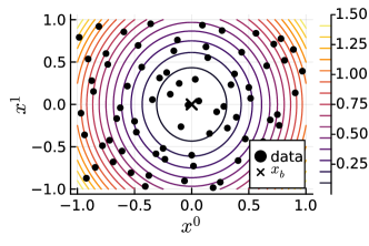
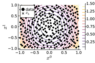
Figure 1: Training data points projected to the $(x^{0},x^{1})$-plane of $\xi_{80}$ (left) and $\xi_{300}$ (right).

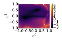
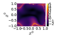
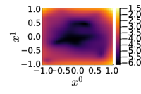
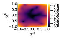
Figure 2: Plots of variances $\log_{10}(\|\mathrm{var}(\mathrm{EL}(\xi_{M}))\|)$ for $M=80$ (two left plots) and $M=300$ (two right plots) over $(x^{0},x^{1},0,0)$-plane and $(x^{0},0,\dot{x}^{0},0)$-plane. (Ranges of colourbars vary.)

Figure 3 shows a motion computed by solving $\mathrm{EL}(L_{M})=0$ with initial data $\overline{x}=(0.2,0.1,0,0)$ on the time interval $[0,100]$. In the plots of the first row, colours indicate the norm of the variance of $\mathrm{EL}(\xi_{M})$ along the computed trajectories. For $M=300$ the trajectory is close to the reference solution while largely different for $M=80$. This is consistent with the lower variance for $M=300$ compared to the experiment with $M=80$. The plots of the dynamics of $L_{300}$ (bottom row of Figure 3) show divergence of the computed motion from the reference solution towards the end of the time interval building up to a difference in $x^{0}$ component of about $0.1$ at $t=100$. (We will see later that a discrete model model performs better in this experiment.) However, the qualitative features of the motion are captured.

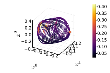
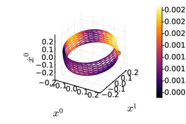
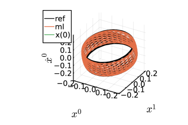
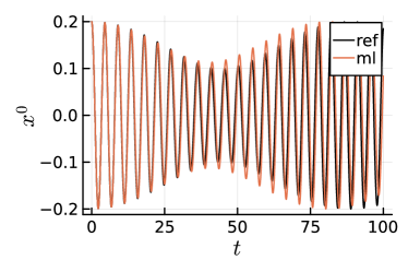
Figure 3: Top row: motion of $\xi_{80}$ (left) and $\xi_{300}$ (right) with variance $\|\mathrm{var}(\mathrm{EL}(\xi_{M}))\|$ encoded as colours (ranges of colourbars vary). Bottom row: motions of $\xi_{300}$ compared to reference.

Figure 4 shows the Hamiltonian $H_{M}=\mathrm{Ham}(L_{M})$ as well as $H_{M}\pm 0.2\sigma_{H_{M}}$. Here $\sigma_{H_{M}}$ denotes the standard deviation $\sqrt{\mathrm{var}\mathrm{Ham}(\xi_{M})}$. We observe a clear decrease of the standard deviation as $M$ increases from 80 to 300.

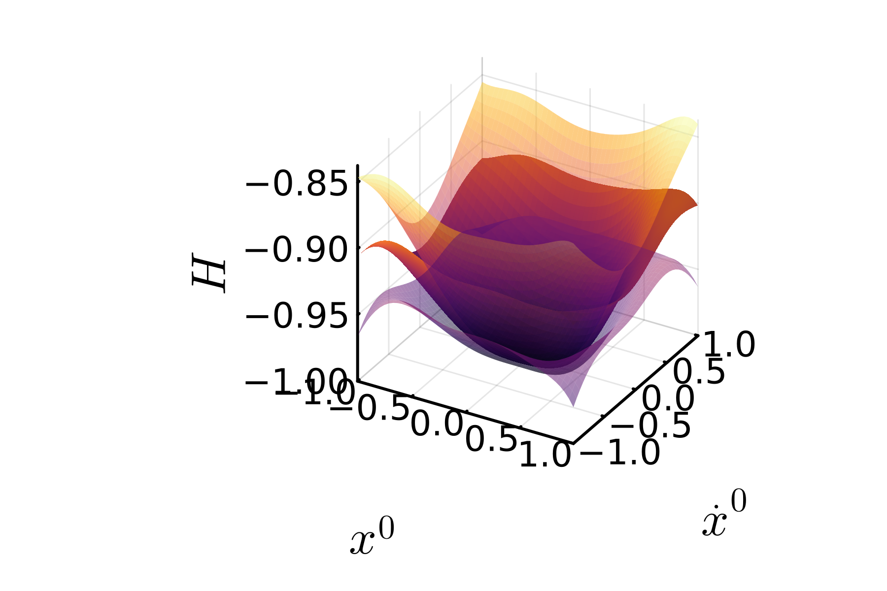
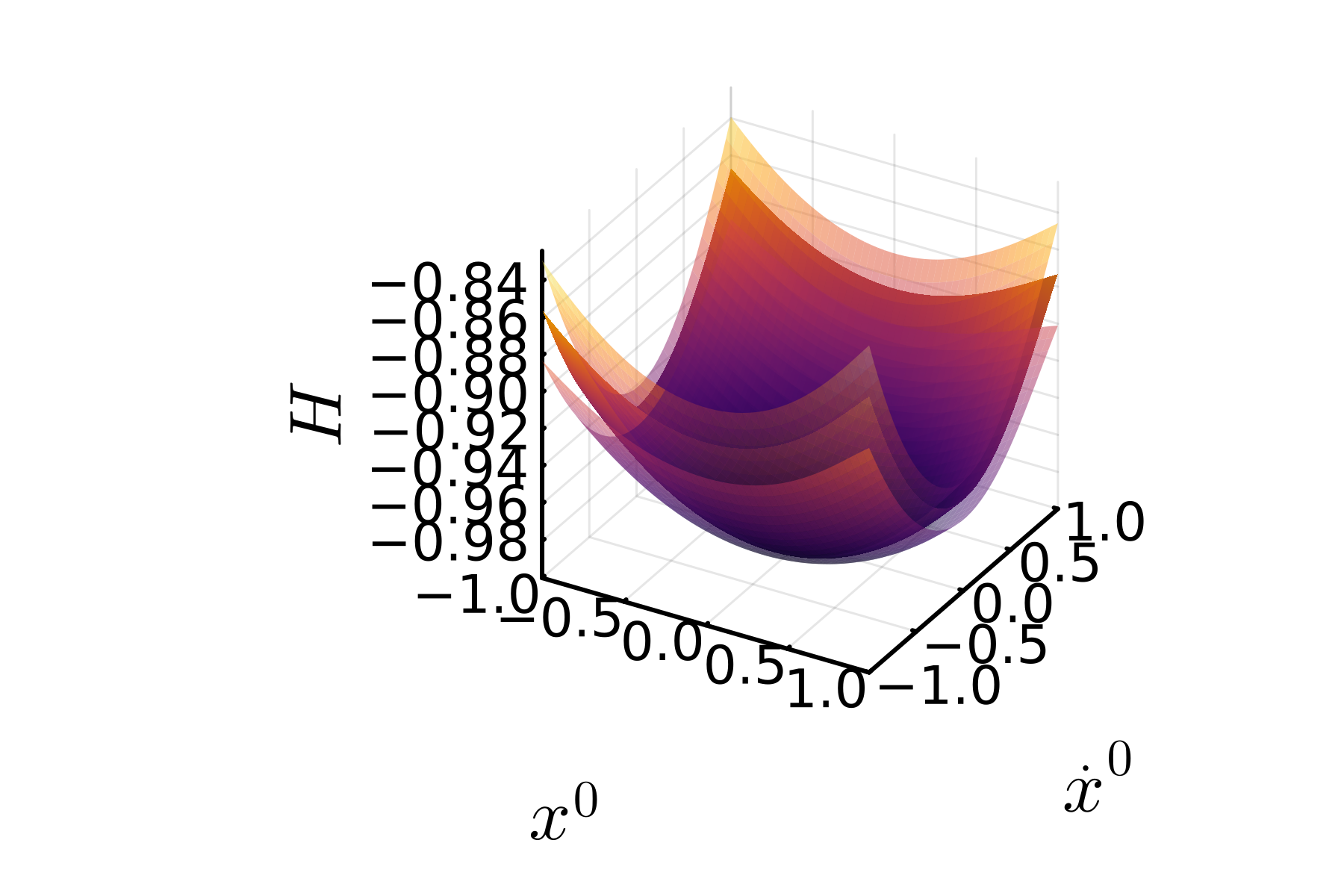
Figure 4: Mean of Hamiltonian $\mathrm{Ham}(\xi_{80})$, $\mathrm{Ham}(\xi_{300})$ over $(x^{0},0,\dot{x}^{0},0)$ plus/minus 20% standard deviation.

Figure 5 displays the error in the prediction of $\ddot{x}$ for points $\overline{x}=(x^{0},x^{1},0,0)\in\Omega$ and $\overline{x}=(x^{0},0,\dot{x}^{0},0)\in\Omega$. As the magnitudes of errors vary widely, $\log_{10}$ is applied before plotting, i.e. we show the quantity

$$\log_{10}\|\mathrm{Acc}_{\overline{x}}(L_{M})-\mathrm{Acc}_{\overline{x}}(L_{{\mathrm{ref}}})\|_{\mathbb{R}^{2}}.$$

One sees a clear decrease in error as $M$ is increased from 80 to 300.

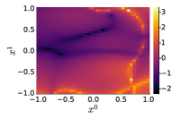
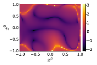
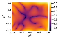
Figure 5: $\log_{10}$ norm of error of predicted acceleration $\ddot{x}$ for $\mathrm{Acc}(\xi_{M})$ over $x^{0},x^{1}$ plane and $x^{0},\dot{x}^{0}$ plane for $M=80$ (left two plots) and $M=300$ (right two plots). (The ranges of colourbars vary.)

Figure 6 shows a convergence plot for the relative error in predicted acceleration $\mathrm{err}_{\mathrm{Acc}}$, i.e. of

$$\mathrm{err}_{\mathrm{Acc}}(\overline{x})=\frac{\|\mathrm{Acc}_{\overline{x}}(L_{M})-\mathrm{Acc}_{\overline{x}}(L_{{\mathrm{ref}}})\|_{\mathbb{R}^{d}}}{\|\mathrm{Acc}_{\overline{x}}(L_{{\mathrm{ref}}})\|_{\mathbb{R}^{d}}}.$$

The data for the plot in Figure 6 was computed for the 1d harmonic oscillator $L_{{\mathrm{ref}}}(x)=\frac{1}{2}\dot{x}^{2}-\frac{1}{2}x^{2}$ with $(x,\dot{x})\in[-1,1]^{2}$ in quadruple precision. For each $M\in\{2^{1},2^{2},\ldots,2^{6}\}$ the error $\mathrm{err}_{\mathrm{Acc}}(\overline{x})$ was evaluated on a uniform mesh with $10\times 11$ mesh points in $[-1,1]\times[-1,1]\in T\mathbb{R}$. The plot shows the discrete $L_{p}$ error ($p=1,2,\infty$). We can see convergence with errors levelling out due to round-off errors at approximately $10^{-11}$.

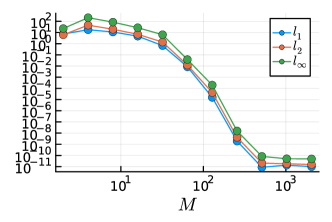
Figure 6: Convergence of $\mathrm{Acc}(L_{M})$ to true acceleration data.

5.2 Discrete Lagrangian

Now we consider dynamical data $\hat{x}^{(j)}=(x^{(j)}_{0},x^{(j)}_{1},x^{(j)}_{2})$ where $x^{(j)}_{0}$, $x^{(j)}_{1}$, $x^{(j)}_{2}$ are snapshots of true trajectories at times $t$, $t+h$, $t+2h$, respectively, with $j=1,\ldots,M$. Here $h=0.1$ and, again, $M\in\{80,300\}$. For data generation, we consider data $(x,p)\in[-1,1]^{4}\subset T^{\ast}\mathbb{R}^{2}$ from a Halton sequence from where we integrate $L_{{\mathrm{ref}}}$ from $[0,3h]$ using the 2nd order accurate variational midpoint rule [23] with step-size $h_{\mathrm{internal}}=h/10$. These dynamics are considered as true for the purpose of this experiment. Training data is visualised in Figure 7.

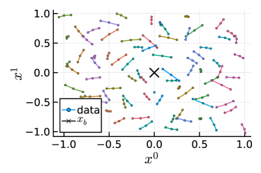
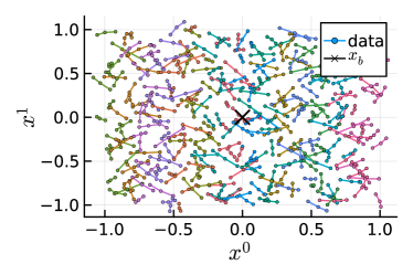
Figure 7: Training data. Each line connects snapshots points that constitute a training data point $\hat{x}$. Left: $M=80$, right: $M=300$.

Figure 8 (in analogy to Figure 2) shows how variance decreases as more data points become available. For the plots, $(x_{0},p_{0})\in T^{\ast}\mathbb{R}^{2}$ are used to compute $\hat{x}=(x_{0},x_{1},x_{2})$ using $L_{{\mathrm{ref}}}$. Here $p$ refers to the conjugate momentum of $L_{{\mathrm{ref}}}$. The plots display heatmaps of $\log_{10}(\|\mathrm{var}(\mathrm{DEL}_{\hat{x}}(\xi_{M}))\|)$.

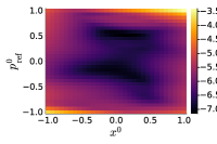
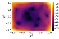
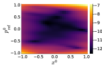
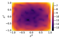
Figure 8: Plots of variances $\log_{10}(\|\mathrm{var}(\mathrm{EL}(\xi_{M}))\|)$ for $M=80$ (left two plots) and $M=300$ (right two plots) over $(x,p_{{\mathrm{ref}}})=(x^{0},x^{1},0,0)$-plane and $(x,p_{{\mathrm{ref}}})=(x^{0},0,p_{{\mathrm{ref}}}^{0},0)$-plane. (Ranges of colourbars vary.)

Figure 9 shows a motion for $t\in[0,100]$ of $\xi_{300}$ with same initial data as in Figure 3. With a maximal error in absolute norm smaller than $0.00043$ it is visually indistinguishable from the true motion. In the plot to the left, data for $\dot{x}^{0}$ was approximated to second order accuracy in $h$ with the central finite differences method.

Comparing Figure 9 and Figure 3, it is interesting to observe that with the same amount of data the discrete model performs better than the continuous model for predicting motions.

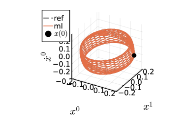
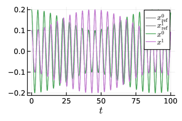
Figure 9: The motion of $\xi_{300}$ and the true motion are indistinguishable.

Reproducibility

Source code of the experiments can be found at https://github.com/Christian-Offen/Lagrangian_GP.

6 Convergence Analysis

This section contains convergence theorems for the considered method for regular continuous Lagrangians (Theorem 1) and discrete Lagrangians (Theorem 2) in the infinite-data limit as observations become topologically dense, i.e. as the maximal distance between data points converges to zero.

6.1 Continuous Lagrangians

6.1.1 Convergence theorem (continuous, temporal evolution)

Theorem 1

Let $\Omega\subset T\mathbb{R}^{d}\cong\mathbb{R}^{d}\times\mathbb{R}^{d}$ be an open, bounded non-empty domain. Consider a sequence of observations $\Omega_{0}^{E}=\{(x^{(j)},\dot{x}^{(j)},\ddot{x}^{(j)})\}_{j}\subset\Omega\times\mathbb{R}^{d}$ of a dynamical system governed by the Euler–Lagrange equation of an (unknown) non-degenerate Lagrangian $L_{{\mathrm{ref}}}\in\mathcal{C}^{2}(\overline{\Omega})$ (definition of $\mathcal{C}^{2}(\overline{\Omega})$ below). Assume that $\{(x^{(j)},\dot{x}^{(j)})\}_{j}\subset\Omega$ is topologically dense. Let $K$ be a 4-times continuously differentiable kernel on $\Omega$, $\overline{x_{b}}\in\Omega$, $r_{b}\in\mathbb{R}$, $p_{b}\in\mathbb{R}$ and assume that $L_{{\mathrm{ref}}}$ is contained in the reproducing kernel Hilbert space $(U,\|\cdot\|_{U})$ to $K$ and fulfils the normalisation condition

$$\Phi_{N}(L_{{\mathrm{ref}}})=(p_{b},r_{b})\quad\text{with}\quad\Phi_{N}(L)=\left(\frac{\partial L}{\partial\dot{x}}(\overline{x}_{b}),L(\overline{x}_{b})\right).$$ (26)

Assume that $U$ embeds continuously into $\mathcal{C}^{2}(\overline{\Omega})$. Let $\xi\in\mathcal{N}(0,\mathcal{K})$ be a canonical Gaussian process on $U$ (see Section 4.1.1). Then the sequence of conditional means $L_{(j)}$ of $\xi$ conditioned on the first $j$ observations and the normalisation conditions

$$\mathrm{EL}(\xi)(x^{(i)},\dot{x}^{(i)},\ddot{x}^{(i)})=0\,(\forall i\leq j),\quad\Phi_{N}(\xi)=(p_{b},r_{b})$$ (27)

converges in $\|\cdot\|_{U}$ and in $\|\cdot\|_{\mathcal{C}^{2}(\overline{\Omega})}$ to a Lagrangian $L_{(\infty)}\in U$ that is

• consistent with the normalisation $\Phi_{N}(L_{(\infty)})=(p_{b},r_{b})$

• consistent with the dynamics, i.e. $\mathrm{EL}(L_{(\infty)})(\hat{x})$ for all $\hat{x}=(x,\dot{x},\ddot{x})$ with $(x,\dot{x})\in\Omega$ and $\mathrm{EL}(L_{{\mathrm{ref}}})(\hat{x})=0$.

• Moreover, $L_{(\infty)}$ is the unique minimiser of $\|\cdot\|_{U}$ among all Lagrangians with these properties.

_□

Remark 6

If $r_{b}=0$ and $p_{b}=0$, then the sequence $L_{(j)}$ is constantly zero with limit $L_{(\infty)}\equiv 0$. It is necessary to set $(r_{b},p_{b})\not=(0,0)$ to approximate a non-degenerate Lagrangian. _□

Remark 7

The regularity assumptions of the kernel (four times continuously differentiable) is required for the interpretation of $L_{(j)}$ as a conditional mean of a Gaussian process and for its convenient computation. However, it be relaxed to twice continuously differentiable as the proof will show. _□

6.1.2 Formal setting and proof (continuous, temporal evolution)

Let $\Omega\subset T\mathbb{R}^{d}$ be an open, bounded, non-empty domain. Following notion of [1], we consider the space of $m$-times continuously differentiable functions that extend to the topological closure $\overline{\Omega}$

$$\mathcal{C}^{m}(\overline{\Omega},\mathbb{R}^{k})=\{f\in\mathcal{C}^{m}(\Omega,\mathbb{R}^{k})\;|\;\partial^{\alpha}f\textrm{ extends continuously to }\overline{\Omega}\;\forall|\alpha|\leq m\},\quad m\in\mathbb{N}_{0}.$$

Here $\partial^{\alpha}f=\frac{\partial^{|\alpha|}f}{(\partial x^{1})^{\alpha_{1}}\ldots(\partial x^{d})^{\alpha_{d}}\partial(\dot{x}^{1})^{\dot{\alpha}_{1}}\ldots(\partial\dot{x}^{d})^{\dot{\alpha}_{d}}}$ denotes the partial derivative with respect to coordinates $\overline{x}=(x,\dot{x})=(x^{1},\ldots,x^{d},\dot{x}^{1},\ldots,\dot{x}^{d})$ for a multi-index $\alpha=(\alpha_{1},\ldots,\alpha_{d},\dot{\alpha}_{1},\ldots,\dot{\alpha}_{d})$ with $|\alpha|=\alpha_{1}+\ldots+\alpha_{d}+\dot{\alpha}_{1}+\ldots+\dot{\alpha}_{d}$. The space is equipped with the norm

$$\|f\|_{\mathcal{C}^{m}(\overline{\Omega},\mathbb{R}^{k})}=\max_{0\leq|\alpha|\leq m}\sup_{\overline{x}\in\Omega}\|\partial^{\alpha}f(\overline{x})\|.\textasciiacute$$ (28)

Here $\|\partial^{\alpha}f(\overline{x})\|$ denotes the Euclidean norm on $\mathbb{R}^{k}$ for $|\alpha|=1$ or an induced operator norm for $|\alpha|>1$. The space $\mathcal{C}^{m}(\overline{\Omega},\mathbb{R}^{k})$ is a Banach space [1, § 4]. We will use the shorthand $\mathcal{C}^{m}(\overline{\Omega})=\mathcal{C}^{m}(\overline{\Omega},\mathbb{R}^{1})$.

Assume that on a dense, countable subset $\Omega_{0}=\{\overline{x}^{(j)}=({x}^{(j)},\dot{x}^{(j)})\}_{j=1}^{\infty}\subset\Omega$ we have observations of acceleration data $\ddot{x}^{(j)}$ of a dynamical system generated by an (a priori unknown) Lagrangian $L_{{\mathrm{ref}}}\in\mathcal{C}^{2}(\overline{\Omega})$, which is non-degenerate, i.e. for all $(x,\dot{x})\in\overline{\Omega}$ the matrix $\frac{\partial^{2}L_{{\mathrm{ref}}}}{\partial\dot{x}\partial\dot{x}}(x,\dot{x})$ is invertible, and the induced function $g_{{\mathrm{ref}}}\in\mathcal{C}^{0}(\overline{\Omega},\mathbb{R}^{d})$ with

$$g_{{\mathrm{ref}}}(x,\dot{x})=\left(\frac{\partial^{2}L_{{\mathrm{ref}}}}{\partial\dot{x}\partial\dot{x}}(x,\dot{x})\right)^{-1}\left(\frac{\partial L_{{\mathrm{ref}}}}{\partial x}(x,\dot{x})-\frac{\partial^{2}L_{{\mathrm{ref}}}}{\partial x\partial\dot{x}}(x,\dot{x})\cdot\dot{x}\right)$$ (29)

recovers $\ddot{x}^{(j)}=g_{{\mathrm{ref}}}(\overline{x}^{(j)})=g_{{\mathrm{ref}}}({x}^{(j)},\dot{x}^{(j)})$.

Lemma 3

The linear functional $\Phi^{(\infty)}\colon\mathcal{C}^{2}(\overline{\Omega})\to\mathcal{C}^{0}(\overline{\Omega},\mathbb{R}^{d})$ with

$$\begin{split}\Phi^{(\infty)}(L)(x,\dot{x})&=\mathrm{EL}(L)(x,\dot{x},g_{{\mathrm{ref}}}(x,\dot{x}))\\ &=\frac{\partial^{2}L}{\partial\dot{x}\partial\dot{x}}(x,\dot{x})\cdot g_{{\mathrm{ref}}}(x,\dot{x})+\frac{\partial^{2}L}{\partial x\partial\dot{x}}(x,\dot{x})\cdot\dot{x}-\frac{\partial L}{\partial x}(x,\dot{x})\end{split}$$ (30)

is bounded. _□

Proof

A direct application of the triangle inequality shows

$$\|\Phi^{(\infty)}(L)\|_{\mathcal{C}^{0}(\overline{\Omega},\mathbb{R}^{d})}\leq\left(\|g_{{\mathrm{ref}}}\|_{\mathcal{C}^{0}(\overline{\Omega},\mathbb{R}^{d})}+\sup_{(x,\dot{x})\in\Omega}\|\dot{x}\|+1\right)\|L\|_{{}_{\mathcal{C}^{2}(\overline{\Omega})}}.$$

_■

Since for each $\overline{x}$ the evaluation functional $\mathrm{ev}_{\overline{x}}\colon f\mapsto f(\overline{x})$ on $\mathcal{C}^{0}(\overline{\Omega},\mathbb{R}^{d})$ is bounded, the following functions constitute bounded linear functionals for $j\in\mathbb{N}$:

$$\Phi_{j} \colon\mathcal{C}^{2}(\overline{\Omega})\to\mathbb{R}^{d},\quad\quad\Phi_{j}(L)=\Phi^{(\infty)}(L)(\overline{x}^{(j)})$$

$$\Phi^{(j)} \colon\mathcal{C}^{2}(\overline{\Omega})\to(\mathbb{R}^{d})^{j},\quad\Phi^{(j)}=(\Phi_{1},\ldots,\Phi_{j}).$$

For a reference point $\overline{x}_{b}\in\Omega$ and for $p_{b}\in\mathbb{R}^{d}$, $r_{b}\in\mathbb{R}$ we define the bounded linear functional

$$\Phi_{N} \colon\mathcal{C}^{2}(\overline{\Omega})\to\mathbb{R}^{d+1},\quad\quad\Phi_{N}(L)=\left(\frac{\partial L}{\partial\dot{x}}(\overline{x}_{b}),L(\overline{x}_{b})\right),$$ (31)

related to our normalisation condition, the shorthands $\Phi_{b}^{(k)}=(\Phi_{1},\ldots,\Phi_{k},\Phi_{N})$ and $\Phi_{b}^{(\infty)}=(\Phi^{(\infty)},\Phi_{N})$, and the data

$$y^{(k)} =(0,\ldots,0,p_{b},r_{b})\in(\mathbb{R}^{d})^{k}\times\mathbb{R}^{d}\times\mathbb{R}$$

$$y^{(\infty)} =(0,p_{b},r_{b})\in\mathcal{C}^{0}(\overline{\Omega},\mathbb{R}^{d})\times\mathbb{R}^{d}\times\mathbb{R}.$$

Assumption 1

Assume that there is a Hilbert space $U$ with continuous embedding $U\hookrightarrow\mathcal{C}^{2}(\overline{\Omega})$ such that

$$\{L\in\mathcal{C}^{2}(\overline{\Omega})\,|\,\Phi_{b}^{(\infty)}(L)=y^{(\infty)}\}\cap U\not=\emptyset$$

In other words, $U$ is assumed to contain a Lagrangian consistent with the normalisation and underlying dynamics.

The affine linear subspace

$$A^{(j)} =\{L\in U\,|\,\Phi_{b}^{(j)}(L)=y^{(j)}\}\quad(j\in\mathbb{N})$$

$$A^{(\infty)} =\{L\in U\,|\,\Phi_{b}^{(\infty)}(L)=y^{(\infty)}\}$$

are closed and non empty in $U$ by Assumption 1 and by the boundedness of $\Phi_{b}^{(j)}$ and $\Phi_{b}^{(\infty)}$ on $U\hookrightarrow\mathcal{C}^{2}(\overline{\Omega})$. Therefore, the following minimisation constitute convex optimisation problems on $B$ with unique minima in $A^{(j)}$ or $A^{(\infty)}$, respectively:

$$\begin{split}L_{(j)}&=\arg\min_{L\in A^{(j)}}\|L\|_{U}\\ L_{(\infty)}&=\arg\min_{L\in A^{(\infty)}}\|L\|_{U}\end{split}$$ (32)

Here $\|\cdot\|_{U}$ denotes the norm in $U$.

Remark 8

In the machine learning setting, $U$ is the reproducing kernel Hilbert space related to a kernel $K\colon\Omega\times\Omega\to\mathbb{R}$. Assume the domain of $\Omega$ is locally Lipschitz. When $K$ is the squared exponential kernel, for instance, its reproducing kernel Hilbert space embeds into any Sobolev space $W^{m}(\Omega)$ ($m>1$) [8, Thm.4.48]. In particular , it embeds into $W^{m}(\Omega)$ with $m>2+d/2$, which is embedded into $\mathcal{C}^{2}(\overline{\Omega})$ by the Sobolev embedding theorem [1, §4]. The element $L_{j}$ from (32) coincides with the conditional mean of the Gaussian process $\xi$ conditioned on $\Phi_{b}^{(j)}(\xi)=y^{(j)}$. _□

Proposition 5

The minima $L_{(j)}$ converge to $L_{(\infty)}$ in the norm $\|\cdot\|_{U}$ and, thus, in $\|\cdot\|_{\mathcal{C}^{2}(\overline{\Omega})}$. _□

Proof

The sequence of affine spaces $A^{(1)}\supseteq A^{(2)}\supseteq A^{(3)}\supseteq\ldots$ is monotonously decreasing and $A^{(\infty)}\subseteq\bigcap_{j=1}^{\infty}A^{(j)}$. Therefore, the sequence $L_{(j)}$ is monotonously increasing and its norm $\|L_{(j)}\|_{U}$ is bounded from above by $\|L_{(\infty)}\|_{U}$. Since $U$ is reflexive, there exists a subsequence $(L_{(j_{i})})_{i\in\mathbb{N}}$ that weakly converges to some $L^{\dagger}_{(\infty)}\in U$. (This follows from the Banach-Alaoglu theorem and the Eberlein-Šmulian theorem [12].) By the weak lower semi-continuity of the norm, we obtain

$$\|L^{\dagger}_{(\infty)}\|_{U}\leq\liminf_{i\to\infty}\|L_{(j_{i})}\|_{U}\leq\|L_{(\infty)}\|_{U}.$$ (33)

Lemma 4

The weak limit $L^{\dagger}_{(\infty)}$ of $(L_{(j_{i})})_{i\in\mathbb{N}}$ is contained in $A^{(\infty)}$. _□

Before providing the proof of Lemma 4, we show how this allows us to complete the proof of Proposition 5.

As $L^{\dagger}_{(\infty)}\in A^{(\infty)}$, we have $\|L_{(\infty)}\|_{U}\leq\|L^{\dagger}_{(\infty)}\|_{U}$ since $L_{(\infty)}$ is the global minimiser of the minimisation problem of (32). Together with (33) we conclude $\|L^{\dagger}_{(\infty)}\|_{U}=\|L_{(\infty)}\|_{U}$ and, by the uniqueness of the minimiser $L_{(\infty)}$, the equality $L^{\dagger}_{(\infty)}=L_{(\infty)}$. Thus, we have proved weak convergence $L_{(j_{i})}\rightharpoonup L_{(\infty)}$.

Together with the lower semi-continuity of the norm, and since $L_{(j_{i})}$ is monotonously increasing and bounded by $\|L_{(\infty)}\|_{U}$, we have

$$\|L_{(\infty)}\|_{U}\leq\liminf_{i\to\infty}\|L_{(j_{i})}\|_{U}\leq\limsup_{i\to\infty}\|L_{(j_{i})}\|_{U}\leq\|L_{(\infty)}\|_{U}$$

such that $\lim_{i\to\infty}\|L_{(j_{i})}\|_{U}=\|L_{(\infty)}\|_{U}$. Together with $L_{(j_{i})}\rightharpoonup L_{(\infty)}$ we conclude strong convergence $L_{(j_{i})}\to L_{(\infty)}$ in the Hilbert space $U$.

The particular weakly convergent subsequence $(L_{(j_{i})})_{i\in\mathbb{N}}$ of $(L_{(j)})_{j}$ was arbitrary. Thus, any weakly convergent subsequence of $(L_{(j)})_{j}$ converges strongly against $L_{(\infty)}$. It follows that any subsequence of $(L_{(j)})_{j}$ has a subsequence that converges to $L_{(\infty)}$. This implies that the whole series $(L_{(j)})_{j}$ converges to $L_{(\infty)}$.

It remains to prove Lemma 4.

Proof (Lemma 4)

Let $\overline{x}\in\Omega$. As the sequence $\Omega_{0}=(\overline{x}^{(m)})_{m=1}^{\infty}$ is dense in $\Omega$, there exists a subsequence $(\overline{x}^{(m_{l})})_{l=1}^{\infty}$ converging to $\overline{x}$. We have

$$\Phi^{(\infty)}_{b}(L^{\dagger}_{(\infty)})(\overline{x}) =\lim_{l\to\infty}\Phi^{(\infty)}_{b}(L^{\dagger}_{(\infty)})(\overline{x}^{(m_{l})})$$ (34)

$$=\lim_{l\to\infty}\underbrace{\lim_{i\to\infty}\Phi^{(\infty)}_{b}(L_{(j_{i})})(\overline{x}^{(m_{l})})}_{\stackrel{{\scriptstyle(\ast)}}{{=}}0}=0.$$ (35)

For this, in (34) we use that $\Phi^{(\infty)}_{b}(L^{\dagger}_{(\infty)})\in\mathcal{C}^{0}(\overline{\Omega})$. Equality in (35) follows because each projection to a component of $\Phi^{(\infty)}_{b}(\cdot)(\overline{x}^{(m_{l})})\colon U\to\mathbb{R}^{d}\times\mathbb{R}^{d+1}$ constitutes a bounded linear functional on $U$ and the sequence $(L_{(j_{i})})_{i\in\mathbb{N}}$ converges weakly to $L^{\dagger}_{(\infty)}$. Finally, equality $(\ast)$ holds because for each $l$ there exists $N\in\mathbb{N}$ such that $j_{N}\geq m_{l}$ and then for all $i\geq N$ we have $\Phi^{(\infty)}_{b}(L_{(j_{i})})(\overline{x}^{(m_{l})})=0$.

From $\Phi^{(\infty)}_{b}(L^{\dagger}_{(\infty)})(\overline{x})=0$ for all $\overline{x}\in\Omega$ we conclude $L^{\dagger}_{(\infty)}\in A^{(\infty)}$. _■

This completes the proof of Proposition 5. _■

Now we can easily prove Theorem 1:

Proof (Theorem 1)

As by general theory (see Remark 4 or [30, Thm 12.5]), the conditional mean $L_{(j)}$ is the unique minimiser of the problem (32). Theorem 1 is, therefore, a direct consequence of Proposition 5. _■

6.2 Discrete Lagrangian

6.2.1 Statement of convergence theorem (discrete, temporal evolution)

Theorem 2

Let $\Omega_{a},\Omega_{b}\subset\mathbb{R}^{d}\times\mathbb{R}^{d}$ be open, bounded, non-empty domains. Let $\Omega=\Omega_{a}\cup\Omega_{b}$. Consider a sequence of observations

$$\hat{\Omega}_{0}=\{\hat{x}^{(j)}=({x_{0}}^{(j)},{x_{1}}^{(j)},{x_{2}}^{(j)})\}_{j=1}^{\infty}$$

of a discrete dynamical system with (not explicitly known) globally Lipschitz continuous discrete flow map $g\colon\Omega_{a}\to\Omega_{b}$ related to a discrete Lagrangian $L_{d}^{{\mathrm{ref}}}\in\mathcal{C}^{1}(\overline{\Omega})$, i.e.

• $g(x_{0}^{(j)},x_{1}^{(j)})=(x_{1}^{(j)},x_{2}^{(j)})$ for all $j\in\mathbb{N}$,

• $\mathrm{DEL}(L_{d}^{{\mathrm{ref}}})(x_{0},g(x_{0},x_{1}))=0$ for all $(x_{0},x_{1})\in\Omega_{a}$,

• $\nabla_{1,2}L_{d}^{{\mathrm{ref}}}(x_{1},x_{2})\in\mathbb{R}^{d\times d}$ is invertible for all $(x_{1},x_{2})\in\overline{\Omega}_{b}$.

Assume that $\{({x_{0}}^{(j)},{x_{1}}^{(j)})\}_{j=1}^{\infty}$ is dense in $\Omega_{a}$. Let $K$ be a twice continuously differentiable kernel on $\Omega$, $\mathcal{u}_{b}\in\Omega$, $r_{b}\in\mathbb{R}$, $p_{b}\in\mathbb{R}$ and assume that $L^{{\mathrm{ref}}}_{d}$ is contained in the reproducing kernel Hilbert space $(U,\|\cdot\|_{U})$ to $K$ and fulfils the normalisation condition

$$\Phi_{N}(L^{{\mathrm{ref}}}_{d})=(p_{b},r_{b})\quad\text{with}\quad\Phi_{N}(L_{d})=\left(-\nabla_{2}L_{d}(\mathcal{u}_{b}),L_{d}(\mathcal{u}_{b})\right)$$ (36)

and that $U$ embeds continuously into $\mathcal{C}^{1}(\overline{\Omega})$. Let $\xi\in\mathcal{N}(0,\mathcal{K})$ be a centred Gaussian random variable over $U$. Then the sequence of conditional means $L_{d,(j)}$ of $\xi$ conditioned on the first $j$ observations and the normalisation conditions

$$\mathrm{DEL}(\xi)(\hat{x}^{(i)})=0\,(\forall i\leq j),\quad\Phi_{N}(\xi)=(p_{b},r_{b})$$ (37)

converges in $\|\cdot\|_{U}$ and in $\|\cdot\|_{\mathcal{C}^{1}(\overline{\Omega})}$ to a Lagrangian $L_{d,(\infty)}\in U$ that is

• consistent with the normalisation $\Phi_{N}(L_{d,(\infty)})=(p_{b},r_{b})$

• consistent with the dynamics, i.e. $\mathrm{DEL}(L_{d,(\infty)})(\hat{x})=0$ for all $\hat{x}=(x_{0},x_{1},x_{2})$ with $(x_{0},x_{1})\in\Omega_{a}$,$(x_{1},x_{2})\in\Omega_{b}$ and $\mathrm{DEL}(L_{d}^{{\mathrm{ref}}})(\hat{x})=0$.

• Moreover, $L_{d}$ is the unique minimizer of $\|\cdot\|_{U}$ among all discrete Lagrangians in $U$ with the properties above.

_□

Remark 9

The regularity assumption of $K$ (twice continuously differentiable) is needed for the interpretation of $L_{d,(j)}$ as a conditional mean of a Gaussian process and for a convenient computation of $L_{d,(j)}$. However, the proof will show that a relaxation to continuous differentiability is possible. _□

6.2.2 Formal setting and proof (discrete, temporal evolution)

Let $\Omega_{a},\Omega_{b}\subset\mathbb{R}^{d}\times\mathbb{R}^{d}$ be open, bounded, non-empty domains, let $\Omega=\Omega_{a}\cup\Omega_{b}$. Let $\hat{\Omega}=\{(x_{0},x_{1},x_{2})\,|\,(x_{0},x_{1})\in\Omega_{a},(x_{1},x_{2})\in\Omega_{b}\}$ and let

$$\hat{\Omega}_{0}=\{(x_{0}^{(j)},x_{1}^{(j)},x_{2}^{(j)})\}_{j=1}^{\infty}\subset\hat{\Omega}\quad\text{with }(x_{0}^{(j)},x_{1}^{(j)})\in\Omega_{a},(x_{1}^{(j)},x_{2}^{(j)})\in\Omega_{b}\;\text{for all }j\in\mathbb{N}.$$

Assume that $\{(x_{0}^{(j)},x_{1}^{(j)})\}_{j=1}^{\infty}$ is dense in $\Omega_{a}$.

Remark 10 (Interpretation of $\hat{\Omega}_{0}$)

The set $\hat{\Omega}_{0}$ corresponds to a collection of observation data in the infinite data limit. It can be obtained as a collection of three consecutive snapshots of motions of the dynamical system that we observe and for which we seek to learn a discrete Lagrangian. In a typical scenario where $L_{d}^{{\mathrm{ref}}}\colon\mathbb{R}^{d}\times\mathbb{R}^{d}\to\mathbb{R}$ is the exact discrete Lagrangian to some underlying continuous Lagrangian, the motions leave the diagonal of $\mathbb{R}^{d}\times\mathbb{R}^{d}$ invariant. It is sensible to consider $\Omega_{a}$ and $\Omega_{b}$ that are neighbourhoods of compact sections of the diagonal in $\mathbb{R}^{d}\times\mathbb{R}^{d}$. _□

We consider the discrete Lagrangian operator

$$\begin{split}&{{\mathrm{DEL}}}\colon\mathcal{C}^{1}(\overline{\Omega})\to\mathcal{C}^{0}(\overline{\hat{\Omega}},\mathbb{R}^{d})\\ &{{\mathrm{DEL}}}(L_{d})(x_{0},x_{1},x_{2})=\nabla_{2}L_{d}(x_{0},x_{1})+\nabla_{1}L_{d}(x_{1},x_{2}).\end{split}$$ (38)

Here $\nabla_{j}L_{d}$ denotes the partial derivatives with respect to the $j$th input argument of $L_{d}$.

Assume that the observations $\hat{\Omega}_{0}=\{(x_{0}^{(j)},x_{1}^{(j)},x_{2}^{(j)})\}_{j=1}^{\infty}$ correspond to a discrete Lagrangian dynamical system governed by $L_{d}^{{\mathrm{ref}}}\in\mathcal{C}^{1}(\overline{\Omega})$ with globally Lipschitz continuous flow map $g\colon\Omega_{a}\to\Omega_{b}$, i.e. ${{\mathrm{DEL}}}(L_{d}^{{\mathrm{ref}}})(x_{0},g(x_{0},x_{1}))=0$ for all $(x_{0},x_{1})\in\Omega_{a}$ and $g(x_{0}^{(j)},x_{1}^{(j)})=(x_{1}^{(j)},x_{2}^{(j)})$ for all $j\in\mathbb{N}$.

Lemma 5

The linear functional $\Phi^{(\infty)}\colon\mathcal{C}^{1}(\overline{\Omega})\to\mathcal{C}^{0}(\overline{\Omega}_{a},\mathbb{R}^{d})$ with

$$\Phi^{(\infty)}(L_{d})(x_{0},x_{1},x_{2})={{\mathrm{DEL}}}(L_{d})(x_{0},g(x_{0},x_{1}))$$ (39)

is bounded. _□

Proof

Indeed, $g$ extends to a globally Lipschitz continuous map $g\colon\overline{\Omega}_{a}\to\overline{\Omega}_{b}$ such that $\Phi^{(\infty)}\colon\mathcal{C}^{1}(\overline{\Omega})\to\mathcal{C}^{0}(\overline{\Omega}_{a},\mathbb{R}^{d})$ is a well-defined map between Banach spaces defined via (39). Let $\|L_{d}\|_{\mathcal{C}^{1}(\overline{\Omega})}\leq 1$. In particular,

$$\sup_{(x_{0},x_{1})\in\Omega_{a}}\|\nabla_{2}L_{d}(x_{0},x_{1})\|\leq 1\quad\text{and}\quad\sup_{(x_{1},x_{2})\in\Omega_{b}}\|\nabla_{2}L_{d}(x_{1},x_{2})\|\leq 1.$$ (40)

Therefore, by the triangle inequality

$$\begin{split}\sup_{(x_{0},x_{1})\in\Omega_{a}}{{\mathrm{DEL}}}(L_{d})(x_{0},g(x_{0},x_{1}))&\leq 1+\sup_{(x_{0},x_{1})\in\Omega_{a}}\|\nabla_{2}L_{d}(g(x_{0},x_{1}))\|\\ &\leq 1+\sup_{(x_{1},x_{2})\in\Omega_{b}}\|\nabla_{2}L_{d}(x_{1},x_{2})\|\leq 2.\end{split}$$ (41)

_■

We can now proceed in direct analogy to the continuous setting (Section 6.1.2) with $L$ replaced by $L_{d}$ and the functional $\Phi_{N}$ of (31) (normalisation conditions) replaced by the corresponding functional for discrete Lagrangians. The details are provided in the following.

Since for each $\overline{x}$ the evaluation functional $\mathrm{ev}_{\overline{x}}\colon f\mapsto f(\overline{x})$ on $\mathcal{C}^{0}(\overline{\Omega}_{a},\mathbb{R}^{d})$ is bounded, the following functions constitute bounded linear functionals for $j\in\mathbb{N}$:

$$\Phi_{j} \colon\mathcal{C}^{1}(\overline{\Omega})\to\mathbb{R}^{d},\quad\quad\Phi_{j}(L_{d})=\Phi^{(\infty)}(L_{d})(\overline{x}^{(j)})$$

$$\Phi^{(j)} \colon\mathcal{C}^{1}(\overline{\Omega})\to(\mathbb{R}^{d})^{j},\quad\Phi^{(j)}=(\Phi_{1},\ldots,\Phi_{j}).$$

For a reference point $\overline{x}_{b}\in\Omega$ and for $p_{b}\in\mathbb{R}^{d}$, $r_{b}\in\mathbb{R}$ we define the bounded linear functional

$$\Phi_{N} \colon\mathcal{C}^{1}(\overline{\Omega})\to\mathbb{R}^{d+1},\quad\quad\Phi_{N}(L)=\left(-\nabla_{1}L_{d}(\overline{x_{b}}),L_{d}(\overline{x}_{b})\right),$$ (42)

related to our normalisation condition for discrete Lagrangians. We will further use the shorthands $\Phi_{b}^{(k)}=(\Phi_{1},\ldots,\Phi_{k},\Phi_{N})$ and $\Phi_{b}^{(\infty)}=(\Phi^{(\infty)},\Phi_{N})$, and define

$$y^{(k)} =(0,\ldots,0,p_{b},r_{b})\in(\mathbb{R}^{d})^{k}\times\mathbb{R}^{d}\times\mathbb{R}$$

$$y^{(\infty)} =(0,p_{b},r_{b})\in\mathcal{C}^{0}(\overline{\Omega},\mathbb{R}^{d})\times\mathbb{R}^{d}\times\mathbb{R}.$$

In analogy to Assumption 1 we consider the following assumption.

Assumption 2

Assume that there is a Hilbert space $U$ with continuous embedding $U\hookrightarrow\mathcal{C}^{1}(\overline{\Omega})$ such that

$$\{L_{d}\in\mathcal{C}^{1}(\overline{\Omega})\,|\,\Phi_{b}^{(\infty)}(L_{d})=y^{(\infty)}\}\cap U\not=\emptyset$$

In other words, $U$ is assumed to contain a Lagrangian consistent with the normalisation and underlying dynamics.

The affine linear subspace

$$A^{(j)} =\{L_{d}\in U\,|\,\Phi_{b}^{(j)}(L_{d})=y^{(j)}\}\quad(j\in\mathbb{N})$$

$$A^{(\infty)} =\{L_{d}\in U\,|\,\Phi_{b}^{(\infty)}(L_{d})=y^{(\infty)}\}$$

are closed in $U$ and not empty by Assumption 2. Therefore, the following extremisation problems constitute convex optimisation problems on $U$ with unique minima in $A^{(j)}$ or $A^{(\infty)}$, respectively:

$$\begin{split}{L_{d}}_{(j)}&=\arg\min_{{L_{d}}\in A^{(j)}}\|{L_{d}}\|_{U}\\ {L_{d}}_{(\infty)}&=\arg\min_{{L_{d}}\in A^{(\infty)}}\|{L_{d}}\|_{U}\end{split}$$ (43)

Here $\|\cdot\|_{U}$ denotes the norm in $U$.

Proposition 6

The minima ${L_{d}}_{(j)}$ converge to ${L_{d}}_{(\infty)}$ in the norm $\|\cdot\|_{U}$ and, thus, in $\|\cdot\|_{\mathcal{C}^{1}(\overline{\Omega})}$. _□

Proof

The proof is in complete analogy to Proposition 5. _■

Proof (Theorem 2)

The unique minimisers $L_{d(j)}$ in (43) are the conditional means considered in Theorem 2 as by Remark 4. Thus, Theorem 2 follows from Proposition 6. _■

7 Summary

We have introduced a method to learn general continuous Lagrangians and discrete Lagrangians from observational data of dynamical system that are governed by variational ordinary differential equations. The method is based on kernel-based, meshless collocation methods for solving partial differential equations [36]. In our context, collocation methods are used to solve the Euler–Lagrange equations that we interpret as a partial differential equations for a Lagrangian function $L$, or discrete Lagrangian $L_{d}$, respectively. Additionally, the use of Gaussian processes gives access to a statistical framework that allows for a quantification of the model uncertainty of the identified dynamical system. This could be used for adaptive sampling of data points. Uncertainty quantification can be efficiently computed for any quantity that is linear in the Lagrangian, such as the Hamiltonian or symplectic structure of the system, which is of relevance in the context of system identification.

The article overcomes the major difficulty that Lagrangians are not uniquely determined by a system’s motions and the presence of degenerate solutions to the Euler–Lagrange equations. This is tackled by a careful consideration of normalisation conditions that reduce the gauge freedom of Lagrangians but do not restrict the generality of the ansatz. Our method profits from implicit regularisation that can be understood as an extremisation of a reproducing kernel Hilbert space norm, based on techniques of game theory [30]. This interpretation as convex optimisation problems is the key ingredient that allows us to provide a rigorous proof of convergence of the method as the maximal distance of observation data points converges to zero.

In future research we will extend the method to dynamical systems governed by variational partial differential equations. Moreover, it is of interest to identify and prove convergence rates of the proposed method. A further direction is the combination with detection methods for Lie group variational symmetries [11, 20] or with detection methods of travelling waves [26, 28]. This may allow for a quantitative analysis of the interplay of symmetry assumptions and model uncertainty.

Data availability

The data that support the findings of this study are openly available in the GitHub repository Christian-Offen/Lagrangian_GP at
https://github.com/Christian-Offen/Lagrangian_GP. An archived version [25] of release v1.0 of the GitHub repository is openly available at https://doi.org/10.5281/zenodo.11093645.

Appendices

Appendix A Alternative regularisation

The following proposition justifies an alternative regularisation strategy. As it involves non-linear conditions, we prefer the regularisation strategy presented in the main body of the document. However, it is presented here for comparison with regularisation strategies for learning of Lagrangian densities using neural networks [28].

Proposition 7

Let $\overline{x}_{b}=(x_{b},\dot{x}_{b})\in T\mathbb{R}^{d}\cong\mathbb{R}^{d}\times\mathbb{R}^{d}$ and $\mathring{L}$ a Lagrangian with $\frac{\partial\mathring{L}}{\partial\dot{x}\partial\dot{x}}(\overline{x}_{b})$ non-degenerate. Let $c_{b}\in\mathbb{R}$, $p_{b}\in\mathbb{R}^{d}$, $c_{\omega}>0$. There exists a Lagrangian $L$ such that $L$ is equivalent to $\mathring{L}$ and

$$L(\overline{x}_{b})=c_{b},\quad\mathrm{Mm}(L)(\overline{x}_{b})=\frac{\partial L}{\partial\dot{x}}(\overline{x}_{b})=p_{b},\quad N_{\omega}(L)(\overline{x}_{b})=\left|\det\left(\frac{\partial^{2}L}{\partial\dot{x}\partial\dot{x}}(\overline{x}_{b})\right)\right|=c_{\omega}.$$ (44)

_□

Proof

Let $\mathring{c_{b}}=\mathring{L}(\overline{x}_{b})$, $\mathring{p_{b}}=\mathrm{Mm}(\mathring{L})(\overline{x}_{b})$, $\mathring{c_{\omega}}=N_{\omega}(\mathring{L})(\overline{x}_{b})$. The quantity $\mathring{c}_{\omega}$ is not zero since $\frac{\partial\mathring{L}}{\partial\dot{x}\partial\dot{x}}(\overline{x}_{b})$ is non-degenerate. We set

$$\rho=\sqrt[d]{\left|\frac{c_{\omega}}{\mathring{c_{\omega}}}\right|},\quad F(x)=x^{\top}(p_{b}-\rho\mathring{p_{b}}),\quad c=c_{b}-\dot{x}_{b}^{\top}(p_{b}-\rho\mathring{p_{b}})-\rho\mathring{c_{b}}.$$

Now the Lagrangian $L=\rho\mathring{L}+\mathrm{d}_{t}F+c$ is equivalent to $\mathring{L}$ and fulfils (14). _■

The condition $N_{\omega}(L)(\overline{x}_{b})=c_{\omega}>0$ may be compared to the regularisation strategies for training Lagrangians modelled as neural networks in [28]: denoting observation data by $\hat{x}^{(j)}=(x^{(j)},\dot{x}^{(j)},\ddot{x}^{(j)})$, in [28] (transferred to our continuous ode setting) parametrises $L$ as a neural network and considers the minimisation of a loss function function $\ell=\ell_{\mathrm{data}}+\ell_{\mathrm{reg}}$ with data consistency term

$$\ell_{\mathrm{data}}=\sum_{j}\|\mathrm{EL}(L)(\hat{x}^{(j)})\|^{2}$$

and with regularisation term $\ell_{\mathrm{reg}}$ that maximises the regularity of the Lagrangian at data points $\hat{x}^{(j)}=(x^{(j)},\dot{x}^{(j)},\ddot{x}^{(j)})$

$$\ell_{\mathrm{reg}}=\sum\left\|\left(\frac{\partial^{2}L}{\partial\dot{x}\partial\dot{x}}(x^{(j)},\dot{x}^{(j)})\right)^{-1}\right\|.$$

The corresponding statement for discrete Lagrangians is as follows.

Proposition 8

Let $\overline{x}_{b}=(x_{0b},x_{1b})\in\mathbb{R}^{d}\times\mathbb{R}^{d}$ and $\mathring{L}_{d}$ a discrete Lagrangian with $\mathrm{Mm}^{-}(\overline{x}_{b})$ non-degenerate. Let $c_{b}\in\mathbb{R}$, $p_{b}\in\mathbb{R}^{d}$, $c_{\omega}>0$. There exists a discrete Lagrangian $L_{d}$ such that $L_{d}$ is equivalent to $\mathring{L}_{d}$ and

$$L_{d}(\overline{x}_{b})=c_{b},\quad\mathrm{Mm}^{-}(L_{d})(\overline{x}_{b})=p_{b},\quad N_{\omega}^{-}(L_{d})(\overline{x}_{b})=\left|\det\left(\frac{\partial^{2}L_{d}}{\partial x_{0}\partial x_{1}}(\overline{x}_{b})\right)\right|=c_{\omega}.$$ (45)

_□

Proof

Let $\mathring{c_{b}}=\mathring{L}_{d}(\overline{x}_{b})$, $\mathring{p_{b}}=\mathrm{Mm}^{-}(\mathring{L}_{d})(\overline{x}_{b})$, $\mathring{c_{\omega}}=N_{\omega}^{-}(\mathring{L}_{d})(\overline{x}_{b})$. The quantity $\mathring{c}_{\omega}$ is not zero since $\frac{\partial\mathring{L}_{d}}{\partial x_{0}\partial x_{1}}(\overline{x}_{b})$ is non-degenerate. We set

$$\rho=\sqrt[d]{\left|\frac{c_{\omega}}{\mathring{c_{\omega}}}\right|},\quad F(x)=x^{\top}(p_{b}-\rho\mathring{p_{b}}),\quad c=c_{b}-\rho\mathring{c_{b}}-(x_{1b}-x_{0b})^{\top}(p_{b}-\rho\mathring{p_{b}}).$$

Now the Lagrangian $L_{d}=\rho\mathring{L}_{d}+\Delta_{t}F+c$ is equivalent to $L_{d}$ and fulfils (45). _■

Again, the condition $N_{\omega}^{-}(L)(\overline{x}_{b})=c_{\omega}>0$ may be compared to the regularisation strategies for training discrete Lagrangians modelled as neural networks in [28]: denoting observation data by $\hat{x}^{(j)}=(x^{(j)}_{0},x_{1}^{(j)},x_{2}^{(j)})$, in [28] (when transferred to our discrete ode setting) parametrises $L_{d}$ as a neural network and considers the minimisation of a loss function function $\ell=\ell_{\mathrm{data}}+\ell_{\mathrm{reg}}$ with data consistency term

$$\ell_{\mathrm{data}}=\sum_{j}\|\mathrm{DEL}(L_{d})(\hat{x}^{(j)})\|^{2}$$

and with regularisation term $\ell_{\mathrm{reg}}$ that maximises the regularity of the Lagrangian at data points $\hat{x}^{(j)}=(x^{(j)}_{0},x_{1}^{(j)},x_{2}^{(j)})$:

$$\ell_{\mathrm{reg}}=\sum\left\|\left(\frac{\partial^{2}L}{\partial x_{0}\partial x_{1}}(x_{0}^{(j)},x_{1}^{(j)})\right)^{-1}\right\|.$$

Appendix B Derivation of symplectic structure induced by discrete Lagrangians

Denote the coordinate of the domain of definition $\mathbb{R}^{d}\times\mathbb{R}^{d}$ of a discrete Lagrangian $L_{d}$ by $(x_{0},x_{1})$. Consider the two discrete Legendre transforms $\Phi^{\pm}\colon\mathbb{R}^{d}\times\mathbb{R}^{d}\to T^{\ast}\mathbb{R}^{d}$ [23] with

$$\Phi^{-}(x_{0},x_{1})=(x_{0},-\frac{\partial L}{\partial x_{0}}(x_{0},x_{1}))\qquad\Phi^{+}(x_{0},x_{1})=(x_{1},\frac{\partial L}{\partial x_{1}}(x_{0},x_{1})).$$

When we pullback the canonical symplectic structure $\sum_{k=1}^{d}\mathrm{d}q^{k}\wedge\mathrm{d}p_{k}$ on $T^{\ast}\mathbb{R}^{d}$ to the discrete phase space $\mathbb{R}^{d}\times\mathbb{R}^{d}$ with $\Phi^{\pm}$ we obtain

$$\mathrm{Sympl}^{-}(L_{d}) =\sum_{s=1}^{d}\mathrm{d}x_{0}^{s}\wedge\mathrm{d}\left(-\frac{\partial L_{d}}{\partial x^{s}_{0}}\right)=\sum_{r,s=1}^{d}-\frac{\partial^{2}L_{d}}{\partial x_{0}^{s}\partial x_{0}^{r}}\mathrm{d}x_{0}^{s}\wedge\mathrm{d}x_{0}^{r}-\frac{\partial^{2}L_{d}}{\partial x_{0}^{s}\partial x_{1}^{r}}\mathrm{d}x_{0}^{s}\wedge\mathrm{d}x_{1}^{r}$$

$$=\sum_{r,s=1}^{d}-\frac{\partial^{2}L_{d}}{\partial x_{0}^{s}\partial x_{1}^{r}}\mathrm{d}x_{0}^{s}\wedge\mathrm{d}x_{1}^{r}$$

$$\mathrm{Sympl}^{+}(L_{d}) =\sum_{s=1}^{d}\mathrm{d}x_{1}^{s}\wedge\mathrm{d}\left(\frac{\partial L_{d}}{\partial x^{s}_{1}}\right)=\sum_{r,s=1}^{d}\frac{\partial^{2}L_{d}}{\partial x_{1}^{s}\partial x_{0}^{r}}\mathrm{d}x_{1}^{s}\wedge\mathrm{d}x_{0}^{r}+\frac{\partial^{2}L_{d}}{\partial x_{1}^{s}\partial x_{1}^{r}}\mathrm{d}x_{1}^{s}\wedge\mathrm{d}x_{1}^{r}$$

$$=\sum_{r,s=1}^{d}\frac{\partial^{2}L_{d}}{\partial x_{1}^{s}\partial x_{0}^{r}}\mathrm{d}x_{1}^{s}\wedge\mathrm{d}x_{0}^{r}$$

We see $\mathrm{Sympl}^{-}(L_{d})=\mathrm{Sympl}^{+}(L_{d})$.

The 2-form corresponds to the notion of a discrete Lagrangian symplectic form in [23, §1.3.2].

References

- [1] Robert A. Adams and John J.F. Fournier. Sobolev Spaces, volume 140 of Pure and Applied Mathematics. Elsevier, 2003. doi:10.1016/S0079-8169(03)80006-5.
- [2] Takehiro Aoshima, Takashi Matsubara, and Takaharu Yaguchi. Deep discrete-time lagrangian mechanics. ICLR SimDL, 5 2021. URL: https://simdl.github.io/files/49.pdf.
- [3] Tom Bertalan, Felix Dietrich, Igor Mezić , and Ioannis G. Kevrekidis. On learning Hamiltonian systems from data. Chaos, 29(12):121107, dec 2019. doi:10.1063/1.5128231.
- [4] J F Carinena and L A Ibort. Non-noether constants of motion. Journal of Physics A: Mathematical and General, 16(1):1, 1 1983. doi:10.1088/0305-4470/16/1/010.
- [5] Renyi Chen and Molei Tao. Data-driven prediction of general Hamiltonian dynamics via learning exactly-symplectic maps. In Marina Meila and Tong Zhang, editors, Proceedings of the 38th International Conference on Machine Learning, volume 139 of Proceedings of Machine Learning Research, pages 1717–1727. PMLR, 18–24 Jul 2021. URL: https://proceedings.mlr.press/v139/chen21r.html, arXiv:arXiv:2103.05632.
- [6] Yifan Chen, Bamdad Hosseini, Houman Owhadi, and Andrew M. Stuart. Solving and learning nonlinear pdes with gaussian processes. Journal of Computational Physics, 447:110668, 2021. doi:10.1016/j.jcp.2021.110668.
- [7] Yuhan Chen, Baige Xu, Takashi Matsubara, and Takaharu Yaguchi. Variational principle and variational integrators for neural symplectic forms. In ICML Workshop on New Frontiers in Learning, Control, and Dynamical Systems, 2023. URL: https://openreview.net/forum?id=XvbJqbW3rf.
- [8] Andreas Christmann and Ingo Steinwart. Kernels and Reproducing Kernel Hilbert Spaces, pages 110–163. Springer New York, New York, NY, 2008. doi:10.1007/978-0-387-77242-4_4.
- [9] Miles Cranmer, Sam Greydanus, Stephan Hoyer, Peter Battaglia, David Spergel, and Shirley Ho. Lagrangian neural networks, 2020. doi:10.48550/ARXIV.2003.04630.
- [10] Marco David and Florian Méhats. Symplectic learning for Hamiltonian neural networks. Journal of Computational Physics, 494:112495, 2023. doi:10.1016/j.jcp.2023.112495.
- [11] Eva Dierkes, Christian Offen, Sina Ober-Blöbaum, and Kathrin Flaßkamp. Hamiltonian neural networks with automatic symmetry detection. Chaos, 33(6):063115, 06 2023. 063115. doi:10.1063/5.0142969.
- [12] Joseph Diestel. Sequences and Series in Banach Spaces. Springer New York, 1984. doi:10.1007/978-1-4612-5200-9.
- [13] Sølve Eidnes and Kjetil Olsen Lye. Pseudo-hamiltonian neural networks for learning partial differential equations. Journal of Computational Physics, 500:112738, 2024. doi:10.1016/j.jcp.2023.112738.
- [14] Giulio Evangelisti and Sandra Hirche. Physically consistent learning of conservative lagrangian systems with gaussian processes. In 2022 IEEE 61st Conference on Decision and Control (CDC). IEEE, 2022. doi:10.1109/CDC51059.2022.9993123.
- [15] I.M. Gelfand, S.V. Fomin, and R.A. Silverman. Calculus of Variations. Dover Books on Mathematics. Dover Publications, 2000.
- [16] Samuel Greydanus, Misko Dzamba, and Jason Yosinski. Hamiltonian Neural Networks. In H. Wallach, H. Larochelle, A. Beygelzimer, F. d’Alché Buc, E. Fox, and R. Garnett, editors, Advances in Neural Information Processing Systems, volume 32. Curran Associates, Inc., 2019. URL: https://proceedings.neurips.cc/paper/2019/file/26cd8ecadce0d4efd6cc8a8725cbd1f8-Paper.pdf, arXiv:1906.01563.
- [17] Marc Henneaux. Equations of motion, commutation relations and ambiguities in the Lagrangian formalism. Annals of Physics, 140(1):45–64, 1982. doi:10.1016/0003-4916(82)90334-7.
- [18] Jianyu Hu, Juan-Pablo Ortega, and Daiying Yin. A structure-preserving kernel method for learning Hamiltonian systems, 2024. arXiv:2403.10070.
- [19] Pengzhan Jin, Zhen Zhang, Aiqing Zhu, Yifa Tang, and George Em Karniadakis. SympNets: Intrinsic structure-preserving symplectic networks for identifying Hamiltonian systems. Neural Networks, 132:166–179, 2020. doi:10.1016/j.neunet.2020.08.017.
- [20] Yana Lishkova, Paul Scherer, Steffen Ridderbusch, Mateja Jamnik, Pietro Liò, Sina Ober-Blöbaum, and Christian Offen. Discrete Lagrangian neural networks with automatic symmetry discovery. IFAC-PapersOnLine, 56(2):3203–3210, 2023. 22nd IFAC World Congress. doi:10.1016/j.ifacol.2023.10.1457.
- [21] G. Marmo and G. Morandi. On the inverse problem with symmetries, and the appearance of cohomologies in classical Lagrangian dynamics. Reports on Mathematical Physics, 28(3):389–410, 1989. doi:10.1016/0034-4877(89)90071-2.
- [22] Giuseppe Marmo and C. Rubano. On the uniqueness of the Lagrangian description for charged particles in external magnetic field. Il Nuovo Cimento A, 98(4):387–399, 10 1987. doi:10.1007/bf02902083.
- [23] Jerrold E. Marsden and Matthew West. Discrete mechanics and variational integrators. Acta Numerica, 10:357–514, 2001. doi:10.1017/S096249290100006X.
- [24] Sina Ober-Blöbaum and Christian Offen. Variational learning of Euler–Lagrange dynamics from data. Journal of Computational and Applied Mathematics, 421:114780, 2023. doi:10.1016/j.cam.2022.114780.
- [25] Christian Offen. Software: Christian-Offen/Lagrangian_GP: Initial release of GitHub Repository, 4 2024. doi:10.5281/zenodo.11093645.
- [26] Christian Offen and Sina Ober-Blöbaum. Learning discrete lagrangians for variational pdes from data and detection of travelling waves. In Frank Nielsen and Frédéric Barbaresco, editors, Geometric Science of Information, volume 14071, pages 569–579, Cham, 2023. Springer Nature Switzerland. doi:10.1007/978-3-031-38271-0_57.
- [27] Christian Offen and Sina Ober-Blöbaum. Symplectic integration of learned Hamiltonian systems. Chaos, 32(1):013122, 1 2022. doi:10.1063/5.0065913.
- [28] Christian Offen and Sina Ober-Blöbaum. Learning of discrete models of variational PDEs from data. Chaos, 34:013104, 1 2024. doi:10.1063/5.0172287.
- [29] Juan-Pablo Ortega and Daiying Yin. Learnability of linear port-Hamiltonian systems, 2023. arXiv:2303.15779.
- [30] Houman Owhadi and Clint Scovel. Operator-Adapted Wavelets, Fast Solvers, and Numerical Homogenization: From a Game Theoretic Approach to Numerical Approximation and Algorithm Design. Cambridge Monographs on Applied and Computational Mathematics. Cambridge University Press, 2019. doi:10.1017/9781108594967.
- [31] Hong Qin. Machine learning and serving of discrete field theories. Scientific Reports, 10(1), 11 2020. doi:10.1038/s41598-020-76301-0.
- [32] Joaquin Quiñonero-Candela and Carl Edward Rasmussen. A unifying view of sparse approximate gaussian process regression. Journal of Machine Learning Research, 6(65):1939–1959, 2005. URL: http://jmlr.org/papers/v6/quinonero-candela05a.html.
- [33] Christopher Rackauckas and Qing Nie. Differentialequations.jl–a performant and feature-rich ecosystem for solving differential equations in julia. Journal of Open Research Software, 5(1):15, 2017. doi:10.5334/jors.151.
- [34] Katharina Rath, Christopher G. Albert, Bernd Bischl, and Udo von Toussaint. Symplectic Gaussian process regression of maps in Hamiltonian systems. Chaos, 31(5):053121, 05 2021. doi:10.1063/5.0048129.
- [35] Tomáš Roubíček. Calculus of Variations, pages 1–38. John Wiley & Sons, Ltd, 2015. doi:10.1002/3527600434.eap735.
- [36] Robert Schaback and Holger Wendland. Kernel techniques: From machine learning to meshless methods. Acta Numerica, 15:543–639, 2006. doi:10.1017/S0962492906270016.
- [37] Florian Schäfer, Matthias Katzfuss, and Houman Owhadi. Sparse Cholesky factorization by Kullback–Leibler minimization. SIAM Journal on Scientific Computing, 43(3):A2019–A2046, 2021. doi:10.1137/20M1336254.
- [38] Mats Vermeeren. Modified equations for variational integrators. Numerische Mathematik, 137(4):1001–1037, 6 2017. doi:10.1007/s00211-017-0896-4.