Consensus + Innovations Approach for Online Distributed Multi-Area Inertia Estimation

Abstract

The reduction of overall system inertia in modern power systems due to the increasing deployment of distributed energy resources is generally recognized as a major issue for system stability. Consequently, real-time monitoring of system inertia is critical to ensure a reliable and cost-effective system operation. Large-scale power systems are typically managed by multiple transmission system operators, making it difficult to have a central entity with access to global measurement data, which is usually required for estimating the overall system inertia. We address this problem by proposing a fully distributed inertia estimation algorithm with rigorous analytical convergence guarantees. This method requires only peer-to-peer sharing of local parameter estimates between neighboring control areas, eliminating the need for a centralized collection of real-time measurements. We robustify the algorithm in the presence of typical power system disturbances and demonstrate its performance in simulations based on the well-known New England IEEE-39 bus system.

I Introduction

The worldwide energy transition is leading to a progressive replacement of conventional synchrounous generators (SGs) by power-electronic interfaced distributed energy resources (DERs) [1, 2, 3]. SGs, which physically provide instantaneous energy reserve through the inertia of their rotating mass, play a key role in smoothing out power fluctuations in the grid. While it is possible to control DERs to support the grid and contribute to the total inertia [1], the vast majority of DERs installed nowadays do not provide inertia. Hence, the total inertia available in power systems decreases [4]. At the same time, new demand-response technologies and increasingly complex loads are installed, resulting in higher and reverse power flows [3]. Consequently, power systems are more frequently operated closer to the stability limits, and the overall dynamics become faster [5]. The European Network of Transmission System Operators for Electricity (ENTSOE) recently identified the decrease in system inertia as the most critical power system stability issue for the continental European grid [6]. As such, tracking the total inertia and assessing the stability of the system becomes increasingly challenging for transmission system operators (TSOs) in the uncertain and deregulated environment of modern power systems [7, 8]. This problem is further aggravated by the fact that large multi-area power systems are typically operated by a number of independent TSOs, each responsible for a separate control area. Since estimating the total inertia usually requires measurement data from the entire system, cooperation among TSOs becomes imperative.

The development of methods for estimating the power system inertia has recently received considerable research attention. The presented schemes follow a centralized approach and can be broadly categorized into offline, online, and forecasting methods [4]. For in-depth discussions, the reader is referred to [4, 9, 10] for recent reviews on the subject. While many promising solutions have been proposed—to the best of the author’s knowledge—no online distributed method with rigorous analytical convergence guarantees and robustness in the presence of disturbances has been presented. In such a way, the application in a practical setting and during different grid operation conditions can be facilitated as only peer-to-peer sharing of local parameter estimates between neighboring control areas is needed, avoiding a central entity and sharing of real-time measurements. This significantly reduces the communication infrastructure required and avoids the potential disclosure of sensitive data.

In this context, we propose an online robust consensus + innovations (C+I)-based distributed parameter estimator (see [11] for a theoretical analysis of the algorithm) for the inertia in multi-area power systems. More precisely, our contributions are three-fold:

• Based on the center of inertia (COI) dynamics of each control area, we derive linear regression equations (LREs) depending only on local measurements, which enable the subsequent distributed parameter estimation scheme.

• We propose a method to estimate in real-time the inertia constants of all control areas and the total inertia of the multi-area power system in a fully distributed manner. Moreover, we analytically establish the global convergence of the parameter estimates to the true parameter vector under standard assumptions. Lastly, we robustify the algorithm in the presence of typical disturbances in power systems, such as parameter variations, measurement noise, and disturbances in the communication channels.

• A simulation study based on the well-known New England IEEE-39 bus system [12], illustrates the effectiveness of the proposed algorithm. It is shown that the method accurately tracks the total inertia and the inertia constants of all control areas at each control area during regular grid operation, even in the presence of various disturbances.

The remainder of this paper is organized as follows. In Section II, the mathematical model of a multi-area power system is presented. Based on that, a robust C+I-based multi-area inertia estimator is introduced in Section III. In Section IV, simulation results are presented. Lastly, in Section V, conclusions and a brief outlook on future work are provided.

II Modeling of multi-area power systems

We consider a large-scale power system with a total of $n>1$ interconnected control areas operated by different TSOs and comprised of $N$ $>$ $1$ SGs. The dynamic behavior of the $i$th SG is represented by a standard swing equation model describing the electromechanical dynamics and given by (see, e.g., [13])

$$\begin{split}\dot{\delta}_{i}(t)&=\Delta\omega_{i}(t)=\omega_{i}(t)-\omega_{\mathrm{s}},\\ \dot{\omega}_{i}(t)&=\frac{\omega_{\mathrm{s}}}{2H_{i}}\left(p_{\mathrm{m},i}(t)-p_{\mathrm{e},i}(t)\right),\end{split}$$ (1)

where the subscript $i$ denotes the variables associated to the $i$th SG, with $\delta_{i}(t)\in\operatorname{\mathbb{R}}$ denoting the rotor angle, $\omega_{i}(t)\in\operatorname{\mathbb{R}_{\geq 0}}$ the shaft speed, $p_{\mathrm{e},i}(t)\in\operatorname{\mathbb{R}_{\geq 0}}$ the electrical air-gap power, the mechanical power $p_{\mathrm{m},i}(t)\in\operatorname{\mathbb{R}_{\geq 0}}$, $\omega_{\mathrm{s}}\in\operatorname{\mathbb{R}_{\geq 0}}$ the nominal synchronous speed, and $H_{i}\in\operatorname{\mathbb{R}_{>0}}$ the inertia constant. To simplify the presentation, in the remainder of the paper, all powers and inertia constants are given in a common global per-unit system. It is assumed that the shaft speed $\omega_{i}$ is close to the nominal synchronous speed $\omega_{s}$, which is a usual assumption in power systems (see, e.g., [13, Chapter 2] and [14, Chapter 5]). Moreover, assuming the stator resistance $R_{\mathrm{s}}$ is zero, the electrical air-gap power $p_{\mathrm{e},i}(t)$ of each SG can be approximated by the terminal electrical power $p_{\mathrm{t},i}(t)\in\operatorname{\mathbb{R}_{\geq 0}}$, which can be measured by the TSO (see, e.g., [15]).

In the following, we consider that the SGs of the power system are strongly coupled to each other. Thus, the COI frequency can be used to represent the principal frequency dynamics of the overall power system. The COI frequency $\omega^{\mathrm{coi}}(t)\in\operatorname{\mathbb{R}_{\geq 0}}$ is defined as (see, e.g., [13, Chapter 2])

$$\omega^{\mathrm{coi}}(t)=\frac{\sum_{i=1}^{N}H_{i}\omega_{i}(t)}{\sum_{i=1}^{N}H_{i}}.$$

As all inertia constants $H_{i}$ are given in the same global per-unit system, the total inertia of the power system $H^{\mathrm{tot}}\in\operatorname{\mathbb{R}_{>0}}$ is calculated as

$$H^{\mathrm{tot}}=\sum_{i=1}^{N}H_{i}.$$

Hence, the dynamics of the COI frequency can be expanded as

$$\dot{\omega}^{\mathrm{coi}}(t)=\frac{\sum_{i=1}^{N}H_{i}\dot{\omega}_{i}(t)}{\sum_{i=1}^{N}H_{i}}=\frac{\omega_{\mathrm{s}}}{{2H^{\mathrm{tot}}}}\left(p_{\mathrm{m}}^{\mathrm{tot}}(t)-p_{\mathrm{e}}^{\mathrm{tot}}(t)\right),$$ (2)

where the total generated electrical power $p_{\mathrm{e}}^{\mathrm{tot}}(t)\in\operatorname{\mathbb{R}_{\geq 0}}$ and the total mechanical power $p_{\mathrm{m}}^{\mathrm{tot}}(t)\in\operatorname{\mathbb{R}_{\geq 0}}$ are defined as

$$p_{\mathrm{e}}^{\mathrm{tot}}(t)=\sum_{i=1}^{N}p_{\mathrm{e},i}(t)\quad\text{and}\quad p_{\mathrm{m}}^{\mathrm{tot}}(t)=\sum_{i=1}^{N}p_{\mathrm{m},i}(t),$$

respectively.

As large-scale power systems are usually operated by several independent TSOs, typically no central entity has access to real-time power and frequency measurements of the overall power system and, hence, estimating the total inertia constant $H^{\mathrm{tot}}$ from (2) is difficult in a practical setting. Nevertheless, the same approach as detailed above can be followed for each control area within a multi-area power system. Here, the COI frequency can be used to represent the principal frequency dynamics of each control area. The COI frequency of the $j$th area $\omega^{\mathrm{coi}}_{j}(t)\in\operatorname{\mathbb{R}_{\geq 0}}$ is given by

$$\omega^{\mathrm{coi}}_{j}(t)=\frac{\sum_{i\in\mathcal{N}^{\mathrm{sg}}_{j}}H_{i}\omega_{i}(t)}{\sum_{i\in\mathcal{N}^{\mathrm{sg}}_{j}}H_{i}},$$ (3)

where the set of SGs in the $j$th control area is denoted by $\mathcal{N}^{\mathrm{sg}}_{j}$. The total inertia of the $j$th area $H^{\mathrm{ca}}_{j}\in\operatorname{\mathbb{R}_{>0}}$ follows from

$$H^{\mathrm{ca}}_{j}=\sum_{i\in\mathcal{N}^{\mathrm{sg}}_{j}}H_{i}.$$

Consequently, the dynamics of the COI frequency of the $j$th area can be expressed as

$$\dot{\omega}^{\mathrm{coi}}_{j}(t)=\frac{\sum_{i\in\mathcal{N}^{\mathrm{sg}}_{j}}H_{i}\dot{\omega}_{i}(t)}{\sum_{i\in\mathcal{N}^{\mathrm{sg}}_{j}}H_{i}}=\frac{\omega_{\mathrm{s}}}{{2H^{\mathrm{ca}}_{j}}}\left(p_{\mathrm{m},j}^{\mathrm{ca}}(t)-p_{\mathrm{e},j}^{\mathrm{ca}}(t)\right),$$ (4)

where the total generated electrical power of the $j$th area $p_{\mathrm{e},j}^{\mathrm{ca}}(t)\in\operatorname{\mathbb{R}_{\geq 0}}$ and the total mechanical power of the $j$th area $p_{\mathrm{m},j}^{\mathrm{ca}}(t)\in\operatorname{\mathbb{R}_{\geq 0}}$ are defined as

$$p_{\mathrm{e},j}^{\mathrm{ca}}(t)=\sum_{i\in\mathcal{N}^{\mathrm{sg}}_{j}}p_{\mathrm{e},i}(t)\quad\text{and}\quad p_{\mathrm{m},j}^{\mathrm{ca}}(t)=\sum_{i\in\mathcal{N}^{\mathrm{sg}}_{j}}p_{\mathrm{m},i}(t),$$

respectively.

If the total inertia constants in all areas are known, the total inertia of the overall power system can be calculated from

$$H^{\mathrm{tot}}=\sum_{j=1}^{n}H^{\mathrm{ca}}_{j}.$$ (5)

As the COI frequency of the $j$th area (3) depends on the unknown inertia constants $H_{i}$, we approximate it by the average frequency of that control area ${\omega}^{\mathrm{av}}_{j}(t)\in\operatorname{\mathbb{R}_{\geq 0}}$ (cf. [16]) as

$${\omega}^{\mathrm{av}}_{j}(t)=\frac{\sum_{i\in\mathcal{N}^{\mathrm{sg}}_{j}}\omega_{i}(t)}{|\mathcal{N}^{\mathrm{sg}}_{j}|},$$ (6)

where $|\mathcal{N}^{\mathrm{sg}}_{j}|$ denotes the cardinality of the set $\mathcal{N}^{\mathrm{sg}}_{j}$, i.e., the number of SGs within the $j$th control area. Then, the dynamics of the COI frequency of the $j$th area (4) can be approximated by the dynamics of the average frequency as

$$\dot{\omega}^{\mathrm{av}}_{j}(t)=\frac{\omega_{\mathrm{s}}}{{2H^{\mathrm{ca}}_{j}}}\left(p_{\mathrm{m},j}^{\mathrm{ca}}(t)-p_{\mathrm{e},j}^{\mathrm{ca}}(t)\right).$$ (7)

As detailed above, the electrical air-gap power $p_{\mathrm{e},i}(t)$ of each SG can be approximated by the terminal electrical power $p_{\mathrm{t},i}(t)$ and, hence, the total generated electrical power of the $j$th control area $p_{\mathrm{e},j}^{\mathrm{ca}}(t)\in\operatorname{\mathbb{R}_{\geq 0}}$ can be approximated as the sum of the terminal electrical powers $p_{\mathrm{t},i}(t)$ via

$$p_{\mathrm{e},j}^{\mathrm{ca}}(t)=\sum_{i\in\mathcal{N}^{\mathrm{sg}}_{j}}p_{\mathrm{t},i}(t).$$

In the following, it is assumed that the TSOs have access to local measurements from their control area. More precisely, the assumption on available measurements is summarized as follows.

Assumption 1.

The system operator of the $j$th control area has access to the signals ${\omega}^{\mathrm{av}}_{j}(t)$, $p_{\mathrm{m},j}^{\mathrm{ca}}(t)$, and $p_{\mathrm{e},j}^{\mathrm{ca}}(t)$.

Remark 1.

The total mechanical power $p_{\mathrm{m},j}^{\mathrm{ca}}(t)$ of the $j$th control area can be composed of a constant and a time-varying part. The constant part depends on the (piecewise) constant power setpoints for each SG within one control area, which are typically known to the respective TSO. The optional time-varying part is due to possible primary-frequency control of some of the SGs and can, e.g., be modeled via a governor and turbine model [16].

Remark 2.

The frequency dynamics of today’s transmission systems, e.g., the synchronous grid of continental Europe, is dominated by SGs. Nevertheless, in modern power systems, SGs are continuously phased out, and at the same time, power-electronics interfaced DERs based on renewable energy sources are implemented in large numbers. Thus, in the future, at least a part of the total inertia has to be provided by DERs through grid-forming control [1]. This can be achieved, e.g., by controlling the DERs to follow the dynamics of the swing equation, as virtual synchronous machines [17] or using droop control [18, 19] among others. Consequently, the frequency dynamics of DERs can be included in the COI frequency dynamics (2) and (4). Differing from the SG model (1), the damping term in DERs under grid-forming control is due to the structure of the control scheme itself (see, e.g., [20, 21]). Hence, it must be incorporated in the COI frequency dynamics as an additional unknown constant, which can be included in the estimation method, e.g., following a similar approach as presented in [22].

III An online robust C+I-based distributed multi-area inertia estimator

In the following, a distributed estimation scheme is developed to reconstruct in real-time the inertia constants $H^{\mathrm{ca}}_{j}$ of all control areas as well as the total inertia constant of the interconnected power system $H^{\mathrm{tot}}$ at each control area using the measurements introduced in Assumption 1.

For this, communication between the control areas is required and it is assumed that neighboring control areas communicate their local parameter estimates with each other in a peer-to-peer fashion. The communication structure among the $n$ control areas is represented by an undirected, time-dependent graph $\mathcal{G}(t)=\left(\mathcal{V},\mathcal{E}(t)\right)$, where $\mathcal{V}=\{1,2,...,n\}$ is the set of nodes, $\mathcal{E}(t)\subseteq\mathcal{V}\times\mathcal{V}$ is the set of edges at time $t$, and the cardinality of $\mathcal{E}(t)$ is denoted by $n_{\mathrm{e}}(t)$. In this way, communication failures can be included in the model as the communication structure is allowed to change over time. The oriented incidence matrix $D(t)\in\mathbb{R}^{n\times n_{\mathrm{e}}(t)}$ is constructed by assigning an arbitrary orientation to the edges of the graph $\mathcal{G}(t)$ at time $t$, and is defined element-wise as $D_{ij}(t)=1$, if $i$ is the source of the $l$th edge, $D_{ij}(t)=-1$, if $i$ is the sink of the $l$th edge, and $D_{ij}(t)=0$ otherwise. The Laplacian matrix $L(t)\in\mathbb{R}^{n\times n}$ of the graph $\mathcal{G}(t)$ at time $t$ is defined as [23]

$$L(t)=D(t)D^{\top}(t).$$ (8)

To obtain LREs, the unknown constants $a^{\mathrm{ca}}_{j}\in\operatorname{\mathbb{R}_{>0}}$ of the $j$th control area and $a^{\mathrm{tot}}\in\operatorname{\mathbb{R}_{>0}}$ of the overall power system are introduced as

$$a^{\mathrm{ca}}_{j}=\frac{\omega_{\mathrm{s}}}{{2H^{\mathrm{ca}}_{j}}},\quad a^{\mathrm{tot}}=\frac{\omega_{\mathrm{s}}}{{2H^{\mathrm{tot}}}}=\frac{1}{{\sum_{j=1}^{n}a^{\mathrm{ca}}_{j}}},$$ (9)

respectively. Hence, by defining the linear second-order filter $\mathcal{F}\in\operatorname{\mathbb{C}}$ as

$$\mathcal{F}(s)=\frac{\lambda_{1}\lambda_{2}}{(\lambda_{1}+s)(\lambda_{2}+s)},$$

with $s$ being the complex frequency domain parameter and $\lambda_{i}\in\operatorname{\mathbb{R}_{>0}},\ i=\{1,2\}$ denoting tuning parameters, a local LRE can be formulated for each control area by applying $\mathcal{F}$ to (7), i.e.,

$$\mathcal{F}\left[s\left[{\omega}^{\mathrm{av}}_{j}\right]\right]=\mathcal{F}\left[p_{\mathrm{m},j}^{\mathrm{ca}}-p_{\mathrm{e},j}^{\mathrm{ca}}\right]a^{\mathrm{ca}}_{j}.$$ (10)

As the aim is to estimate all inertia constants of all control areas, the parameter vector $\theta\in\operatorname{\mathbb{R}}^{n}$ to be estimated is defined as follows

$$\theta=\begin{bmatrix}a^{\mathrm{ca}}_{1}&a^{\mathrm{ca}}_{2}&\dots&a^{\mathrm{ca}}_{n}\end{bmatrix}^{\top}.$$

Furthermore, we define the local output $y_{j}\in\operatorname{\mathbb{R}}$ of the $j$th control area as $y_{j}\coloneqq\mathcal{F}\left[s\left[{\omega}^{\mathrm{av}}_{j}\right]\right],$ and $\nu_{j}\in\operatorname{\mathbb{R}}$ as $\nu_{j}$  $\coloneqq$ $\mathcal{F}\left[p_{\mathrm{m},j}^{\mathrm{ca}}-p_{\mathrm{e},j}^{\mathrm{ca}}\right].$ Then, the local LRE (10) for the $j$th control area can be expressed in dependence of the global parameter vector $\theta$ in the form of the following LRE

$$y_{j}=c_{j}\theta,$$

where $c_{j}\in\operatorname{\mathbb{R}}^{1\times n}$ denotes the regressor of the $j$th control area and is defined as

$$c_{j}\coloneqq\begin{cases}\begin{bmatrix}\nu_{1}&{0}^{\top}_{(n-1)}\end{bmatrix}&\mathrm{for}\ j=1,\vspace{0.1cm}\\ \begin{bmatrix}{0}^{\top}_{(n-1)}&\nu_{n}\end{bmatrix}&\mathrm{for}\ j=n,\vspace{0.1cm}\\ \begin{bmatrix}{0}^{\top}_{(j-1)}&\nu_{j}&{0}^{\top}_{(n-j)}\end{bmatrix}&\mathrm{otherwise},\end{cases}$$

with ${0}_{h}$ representing a $h\times 1$ vector of zeros.

The goal is to estimate consistent parameters $\theta$ at all control areas, which can be achieved by a C+I-type distributed parameter estimation algorithm [24, 11]. With this algorithm, each control area $j$ continuously updates its local estimate $\hat{\theta}_{j}\in\operatorname{\mathbb{R}}^{n}$ using

$$\dot{\hat{\theta}}_{j}=-\alpha\Gamma_{j}\sum_{k\in\mathcal{N}_{j}}(\hat{\theta}_{j}-\hat{\theta}_{k})-\Gamma_{j}c_{j}^{\top}\left(c_{j}\hat{\theta}_{j}-y_{j}\right),$$ (11)

where $\mathcal{N}_{j}$ denotes the set of neighbors of the $j$th control area at time $t$, $\Gamma_{j}\in\mathbb{R}^{n\times n}$ is the gradient descent gain matrix of the $j$th control area, and $\alpha\in\mathbb{R}$ is the additional consensus gain. Notably, this algorithm only requires the communication of the local inertia estimates to neighboring control areas without the need to disclose the underlying local frequency and power measurements.

For establishing the convergence properties of the parameter estimates $\hat{\theta}_{j}\ \forall j=\{1,\cdots,n\}$ in (11), the subsequent standard assumptions are imposed.

Assumption 2.

1. The cooperative Persistency of Excitation condition is fulfilled, i.e., there exist positive constants $T$, $\bar{\iota}_{1}\geq\underline{\iota}_{1}>0$, all independent of $t$, such that for all $t\geq T$ it holds that

   $$\bar{\iota}_{1}I_{N}\geq\int_{t-T}^{t}\sum_{j=1}^{n}c_{j}^{\top}(s){c_{j}}(s)\mathrm{d}s\geq\underline{\iota}_{1}I_{N}.$$

2. All the local regressors are uniformly upper-bounded in the norm, with the upper bound given by $r_{2}>0$, i.e., $\|c_{j}^{\top}(t)c_{j}(t)\|\leq r_{2}\quad\forall\,t\geq 0\quad\forall j=\{1,\cdots,n\}.$

3. The graph $\mathcal{G}(t)$ is connected on average, meaning that $\int_{t-T}^{t}L(s)\mathrm{d}s$, with $T$ as in Assumption 2.1, has only one zero eigenvalue $\lambda_{1}$, and all remaining ones are positive and accept a lower bound denoted by the constant $0<\underline{\lambda}\leq\lambda_{k}(t)\quad\forall k\geq 2$. Furthermore, the time-varying Laplacian $L(t)$ in (8) is uniformly upper-bounded in the norm, with upper bound $r_{3}>0$, i.e., $\|L(t)\|\leq r_{3}\quad\forall\,t\geq 0.$

4. For each control area, its gradient descent gain matrix $\Gamma_{j}$ in (11) is symmetric and positive definite, with the upper bound given by $r_{1}>0$, i.e., $\|\Gamma_{j}\|\leq r_{1}\quad\forall j=\{1,\cdots,n\}.$ Moreover, the additional consensus gain $\alpha$ in (11) is chosen to be strictly positive.

In the literature, Assumption 2 is widely used and is in line with standard practice (see, e.g., [25] for Assumption 2.2, [24] for Assumption 2.1 and Assumption 2.3, while Assumption 2.4 can always be satisfied by proper design). With Assumption 2, global convergence of the estimates $\hat{\theta}_{j}\ \forall j=\{1,\cdots,n\}$ in (11) to the true parameter vector $\theta$, follows by invoking [11, Theorem 1].

From (9), the online estimate of the unknown parameter vector at the $j$th control area $\hat{\theta}_{j}$ can be directly used to estimate the unknown constant of the overall power system $a^{\mathrm{tot}}_{j}$ at the $j$th control area via

$$\hat{a}^{\mathrm{tot}}_{j}=\frac{1}{\sum_{i=1}^{n}\frac{1}{\hat{\theta}_{j,i}}},$$

where $\hat{\theta}_{j,i}\in\operatorname{\mathbb{R}}$ denotes the $i$th component of the parameter estimate at the $j$th control area. Hence, at each control area, the inertia constants $H^{\mathrm{ca}}_{j}$ of all control areas as well as the total inertia constant of the interconnected power system $H^{\mathrm{tot}}$ can be reconstructed accurately by employing (9).

Moreover, following [11, Corollary 4], the gains of the distributed multi-area inertia estimator $\bar{\Gamma}=\operatorname{diag}\left(\Gamma_{1},\cdots,\Gamma_{n}\right)$ and $\alpha$ in (11) can be tuned systematically. In this way, the $\mathcal{L}_{2}$-gain from a disturbance input to a specified performance output can be minimized utilizing the semi-definite program provided in [11, Corollary 4]. Thus, the proposed algorithm (11) can be robustified in the presence of typical disturbances, such as measurement noise, disturbances in the communication channels, and parameter variations. Due to space limitations, the exact procedure is not explained here, but follows the one described in [11]. Hence, the interested reader is referred to [11] for further details.

IV Simulation results

In this section, simulation results utilizing the C+I-based multi-area inertia estimator introduced in (11) are presented. For this, the well-known New England IEEE 39 bus system [12] is used with the SGs modeled via a 9-dimensional model including automatic voltage regulators and power system stabilizers. The power system is divided into three control areas. The SG 1 models the interconnection to an external power grid and, therefore, has a very large inertia constant [26]. Hence, control area 1 is assumed to be the external grid and contains only SG 1. Control area 2 comprises SGs 2-7, and control area 3 contains SGs 8-10. A schematic representation of the considered control areas and the communication topology is depicted in Figure 1.

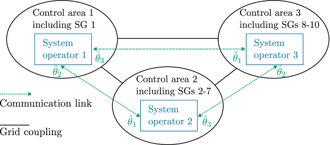
Figure 1: Schematic representation of the considered control areas and the communication topology.

To validate the performance of the method during regular grid conditions, load variations are introduced. The resulting frequencies at all buses are in the range of $60\pm 0.05$ Hz, which is consistent with the typical operation of transmission grids [27]. The available measurements satisfy Assumption 1, i.e., the system operator of the $j$th control area can measure ${\omega}^{\mathrm{av}}_{j}$, $p_{\mathrm{m},j}^{\mathrm{ca}}$, and $p_{\mathrm{e},j}^{\mathrm{ca}}$. Furthermore, initially, all areas communicate their local inertia estimates with all other areas.

To validate the performance of the proposed inertia estimator, we consider a scenario in which the inertia constant at the control area 1 is slowly time-varying. As control area 1 models the interconnection to an external grid, it is assumed that not only SGs but also modern DERs contribute to the total inertia of this sub-grid. Since modern DERs do not provide inertia through the physical inertia of the rotating mass as in the case of SGs, but through the control scheme applied in the form of virtual inertia, their inertia contribution may not be constant or even designed to be time-varying [28, 29, 30]. Additionally, the inertia constant of control area 1 is reduced stepwise at $t=40$ s, resembling, e.g., a disconnection of a large SG. Furthermore, the communication is disturbed by removing the communication link between control area 2 and control area 3 for $t\geq 5$ s. Nevertheless, the graph modeling the communication topology remains connected. Lastly, we consider three cases with varying measurement noise: A nominal, i.e., noisefree case, a case with zero mean Gaussian noise, and a case with zero mean Laplacian noise added to the measurements. In [31], Laplacian noise was recommended to simulate realistic measurement errors. The signal-to-noise ratio of the measurement noise is set to $58$ dB and $95$ dB for the active power and frequency measurements, respectively. These values were determined to resemble the noise power in real-world applications by analyzing measurements from the German extra-high voltage grid obtained in [32]. To achieve robust performance in the presence of these disturbances, the gains of the algorithm are tuned using [11, Corollary 4]. The optimal gains found with this procedure are $\bar{\Gamma}^{*}=2.45I_{n^{2}}$ and $\alpha^{*}=0.4$. All simulations are carried out using MATLAB and the Julia programming language.

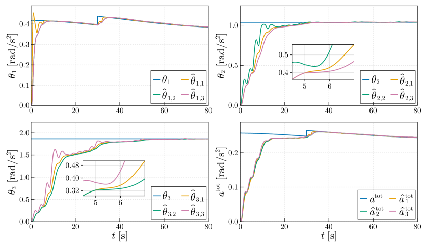
(a) Case 1: Noisefree measurements.

(b) Case 2: Measurements disturbed by zero mean Gaussian noise.

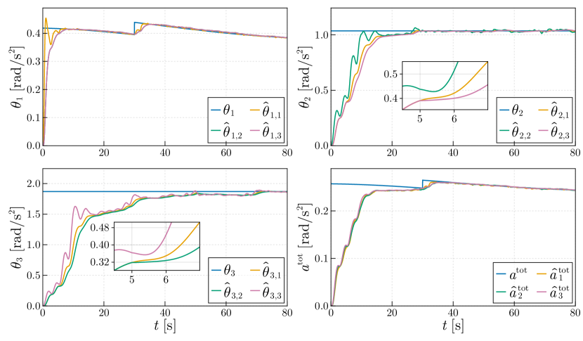
(c) Case 3: Measurements disturbed by zero mean Laplacian noise.

Figure 2: Distributed inertia estimation in the presence of load variations with time-varying inertia at control area 1 and a loss of the communication link between control area 2 and 3 for $t\geq 5$ s.

The simulation results for all three cases are shown in Figure 2. It can be seen that the distributed multi-area inertia estimator, in (11), can accurately estimate the unknown parameters of all control areas and of the overall power system at all control areas. Initially and after the step change at $t=40$ s, the estimation of the time-varying parameter of control area 1 converges very quickly. The convergence of the estimation of the unknown parameters of control areas 2 and 3 takes slightly longer. The disturbance in the communication, i.e., the failure of the communication link between control areas 2 and 3 for $t\geq 5$ s, yields a delay in the estimation, which is most visible in the estimation of the unknown parameters of control areas 2 and 3. As seen from the zoomed-in plot at around $t=5$ s, the values of $\hat{\theta}_{2,1}$ and $\hat{\theta}_{2,2}$ as well as of $\hat{\theta}_{3,1}$ and $\hat{\theta}_{3,2}$ deviate from each other as the information can not be shared via the lost communication link anymore and travels a further way, i.e., via control area 1. As the graph describing the communication topology remains connected even after the loss of the communication link, the estimates still converge at all control areas. Overall, the robust distributed multi-area inertia estimator performs very well in all cases and is capable of correctly estimating the unknown parameters even in the presence of disturbances.

V Conclusions and future work

In this work, we presented a novel C+I-based online robust distributed inertia estimation method for multi-area power systems with rigorous analytical convergence guarantees. We are not aware of any other fully distributed scheme addressing this problem, i.e., without requiring a central entity with access to global measurement information. This is especially relevant as large-scale interconnected power systems are usually operated by multiple independent TSOs. Therefore, having a centralized inertia estimation entity may be difficult in a practical setting due to the potential disclosure of sensitive data and because it requires an elaborate infrastructure for real-time sharing of measurements. Instead, the proposed method requires only peer-to-peer sharing of local parameter estimates between neighboring control areas. In this way, sharing of the actual measurement data is not necessary.

More specifically, we derived a LRE from the COI frequency model for each control area, which allowed us to apply a C+I-based distributed parameter estimator to this problem setup. We analytically proved the Global Exponential Stability (GES) of the origin of the resulting error dynamics and robustified the algorithm in the presence of typical disturbances in power systems. Lastly, the algorithm was validated using simulation results based on the well-known New England IEEE 39 bus system. Here, the method could accurately reconstruct the inertia constants in the presence of communication disturbances, measurement noise, and variations in the inertia constant of the external grid.

In the future, we plan to validate the method in a large-scale simulation study based on a dynamic 1013-machine ENTSOE model through several test cases.

References

- [1] F. Dörfler and D. Groß, “Control of Low-Inertia Power Systems,” Annual Review of Control, Robotics, and Autonomous Systems, vol. 6, pp. 415–445, May 2023.
- [2] M. Paolone, T. Gaunt, X. Guillaud, M. Liserre, S. Meliopoulos, A. Monti, T. Van Cutsem, V. Vittal, and C. Vournas, “Fundamentals of power systems modelling in the presence of converter-interfaced generation,” Electric Power Systems Research, vol. 189, p. 106811, 2020.
- [3] W. Winter, K. Elkington, G. Bareux, and J. Kostevc, “Pushing the Limits: Europe’s New Grid: Innovative Tools to Combat Transmission Bottlenecks and Reduced Inertia,” IEEE Power and Energy Magazine, vol. 13, pp. 60–74, Jan. 2015.
- [4] E. Heylen, F. Teng, and G. Strbac, “Challenges and opportunities of inertia estimation and forecasting in low-inertia power systems,” Renewable and Sustainable Energy Reviews, vol. 147, p. 111176, 2021.
- [5] F. Milano, F. Doerfler, G. Hug, D. J. Hill, and G. Verbic, “Foundations and Challenges of Low-Inertia Systems (Invited Paper),” in 2018 Power Systems Computation Conference (PSCC), pp. 1–25, June 2018.
- [6] P. Christensen, et al., “High Penetration of Power Electronic Interfaced Power Sources and the Potential Contribution of Grid Forming Converters,” tech. rep., ENTSO-E Technical Group on High Penetration of Power Electronic Interfaced Power Sources, Belgium, 2020.
- [7] A. Ulbig, T. S. Borsche, and G. Andersson, “Impact of Low Rotational Inertia on Power System Stability and Operation,” IFAC Proceedings Volumes, vol. 47, pp. 7290–7297, Jan. 2014.
- [8] E. Ørum, “Future system inertia,” tech. rep., Brussels, Belgium, 2015.
- [9] K. Prabhakar, S. K. Jain, and P. K. Padhy, “Inertia estimation in modern power system: A comprehensive review,” Electric Power Systems Research, vol. 211, p. 108222, Oct. 2022.
- [10] B. Tan, J. Zhao, M. Netto, V. Krishnan, V. Terzija, and Y. Zhang, “Power system inertia estimation: Review of methods and the impacts of converter-interfaced generations,” International Journal of Electrical Power & Energy Systems, vol. 134, p. 107362, Jan. 2022.
- [11] N. Lorenz-Meyer, J. G. Rueda-Escobedo, J. A. Moreno, and J. Schiffer, “A robust consensus + innovations-based distributed parameter estimator,” 2024. Unpublished. Preprint available in arXiv:2401.14158.
- [12] I. Hiskens, “IEEE PES Task Force on Benchmark Systems for Stability Controls,” technical report, 2013.
- [13] G. Andersson, Dynamics and Control of Electric Power Systems. Lecture Notes, ETH Zürich, 2012.
- [14] J. Machowski, B. Janusz W., and B. James R., Power System Dynamics: Stability and Control. West Sussex, United Kingdom: John Wiley & Sons, second ed., 2008.
- [15] E. Ghahremani and I. Kamwa, “Local and Wide-Area PMU-Based Decentralized Dynamic State Estimation in Multi-Machine Power Systems,” IEEE Transactions on Power Systems, vol. 31, pp. 547–562, Jan. 2016.
- [16] J. Schiffer, P. Aristidou, and R. Ortega, “Online Estimation of Power System Inertia Using Dynamic Regressor Extension and Mixing,” IEEE Transactions on Power Systems, vol. 34, no. 6, pp. 4993–5001, 2019.
- [17] S. D’Arco and J. A. Suul, “Virtual synchronous machines — Classification of implementations and analysis of equivalence to droop controllers for microgrids,” in 2013 IEEE Grenoble Conference, pp. 1–7, June 2013.
- [18] E. Barklund, N. Pogaku, M. Prodanovic, C. Hernandez-Aramburo, and T. Green, “Energy Management in Autonomous Microgrid Using Stability-Constrained Droop Control of Inverters,” IEEE Transactions on Power Electronics, vol. 23, pp. 2346–2352, Sept. 2008.
- [19] J. Schiffer, R. Ortega, A. Astolfi, J. Raisch, and T. Sezi, “Conditions for stability of droop-controlled inverter-based microgrids,” Automatica, vol. 50, pp. 2457–2469, Oct. 2014.
- [20] C. Schöll and H. Lens, “Design- and simulation-based comparison of grid-forming converter control concepts,” in Proceedings of the 20th Wind Integration Workshop, (Germany), pp. 310–316, IET, 2021.
- [21] J. Schiffer, D. Goldin, J. Raisch, and T. Sezi, “Synchronization of droop-controlled microgrids with distributed rotational and electronic generation,” in 52nd IEEE Conference on Decision and Control, (Firenze), pp. 2334–2339, IEEE, Dec. 2013.
- [22] N. Lorenz-Meyer, A. Bobtsov, R. Ortega, N. Nikolaev, and J. Schiffer, “PMU-based decentralised mixed algebraic and dynamic state observation in multi-machine power systems,” IET Generation, Transmission & Distribution, vol. 14, no. 25, pp. 6267–6275, 2020.
- [23] F. Bullo, Lectures on Network Systems, vol. 1. Kindle Direct Publishing, 2020.
- [24] W. Chen, C. Wen, S. Hua, and C. Sun, “Distributed Cooperative Adaptive Identification and Control for a Group of Continuous-Time Systems With a Cooperative PE Condition via Consensus,” IEEE Transactions on Automatic Control, vol. 59, pp. 91–106, Jan. 2014.
- [25] J. G. Rueda-Escobedo and J. A. Moreno, “Strong Lyapunov functions for two classical problems in adaptive control,” Automatica, vol. 124, p. 109250, 2021.
- [26] D. Linaro, F. Bizzarri, D. del Giudice, C. Pisani, G. M. Giannuzzi, S. Grillo, and A. M. Brambilla, “Continuous estimation of power system inertia using convolutional neural networks,” Nature Communications, vol. 14, p. 4440, July 2023.
- [27] T. Weissbach, Verbesserung des Kraftwerks- und Netzregelverhaltens bezüglich handelsseitiger Fahrplanänderungen. PhD thesis, University of Stuttgart, 2009.
- [28] G. S. Misyris, S. Chatzivasileiadis, and T. Weckesser, “Robust Frequency Control for Varying Inertia Power Systems,” in 2018 IEEE PES Innovative Smart Grid Technologies Conference Europe, (Sarajevo), pp. 1–6, IEEE, Oct. 2018.
- [29] J. Chen, M. Liu, F. Milano, and O’Donnell, “Adaptive virtual synchronous generator considering converter and storage capacity limits,” CSEE Journal of Power and Energy Systems, vol. 8, no. 2, pp. 580–590, 2020.
- [30] M. Liu, J. Chen, and F. Milano, “On-Line Inertia Estimation for Synchronous and Non-Synchronous Devices,” IEEE Transactions on Power Systems, vol. 36, pp. 2693–2701, May 2021.
- [31] S. Wang, J. Zhao, Z. Huang, and R. Diao, “Assessing Gaussian Assumption of PMU Measurement Error Using Field Data,” IEEE Transactions on Power Delivery, vol. 33, pp. 3233–3236, Dec. 2018.
- [32] N. Lorenz-Meyer, R. Suchantke, and J. Schiffer, “Dynamic state and parameter estimation in multi-machine power systems—Experimental demonstration using real-world PMU-measurements,” Control Engineering Practice, vol. 135, p. 105491, 2023.