Time, Travel, and Energy in the Uniform Dispersion Problem

Abstract

We investigate the algorithmic problem of uniformly dispersing a swarm of robots in an unknown, gridlike environment. In this setting, our goal is to comprehensively study the relationships between performance metrics and robot capabilities. We introduce a formal model comparing dispersion algorithms based on makespan, traveled distance, energy consumption, sensing, communication, and memory. Using this framework, we classify several uniform dispersion algorithms according to their capability requirements and performance. We prove that while makespan and travel can be minimized in all environments, energy cannot, as long as the swarm’s sensing range is bounded. In contrast, we show that energy can be minimized even by simple, “ant-like” robots in synchronous settings and asymptotically minimized in asynchronous settings, provided the environment is topologically simply connected. Our findings offer insights into fundamental limitations that arise when designing swarm robotics systems for exploring unknown environments, highlighting the impact of environment’s topology on the feasibility of energy-efficient dispersion.

I Introduction

In hazardous unknown environments such as collapsed buildings or leaking chemical factories, the deployment of human teams for mapping, search and rescue, or data gathering can be ineffective and dangerous. In recent years, swarm robotics, which involves the use of numerous simple robots working together to achieve a common goal, has emerged as a promising solution for exploring and monitoring such environments. The promise of swarm robotics is that a large number of cheap, expendable robots guided by local sensing-based algorithms and signals can adapt to such environments on the fly, offering an alternative to human intervention [1, 2].

A notable approach to using swarms for exploration and monitoring is the concept of ”flooding” or ”uniform dispersion” [3, 4, 5, 6, 7, 8, 9, 10]. This approach involves gradually deploying a swarm of small, expendable robotic agents at a fixed entry point in the environment and allowing them to explore and settle until the area is fully covered. By operating autonomously and in parallel, these robots can efficiently gather crucial data while reducing the risk to human personnel [8]. Potential applications range from search and rescue missions and environmental monitoring to scientific exploration.

In this work, we study the algorithmic problem the heart of such an approach: flooding an unknown, discrete grid-like environment with a swarm of robots that gradually enter from a source location. This problem, known in the literature as the uniform dispersion problem, was formally posed by Hsiang et al. [3] (building on the earlier work of Howard et al. [11]) and has attracted significant attention in the literature–see “Related Work”. By studying the uniform dispersion problem in a formal mathematical setting, we can gain insights into the fundamental trade-offs and limitations of swarm robotics algorithms, which can inform the design of such systems.

A good uniform dispersion algorithm must try to optimize one or more key metrics:

1. Makespan: The time it takes for the swarm to fully cover the environment.

2. Travel: The distance traveled by each robot, which impacts, e.g., wear on the robots.

3. Energy: The energy consumed by each robot during the exploration process. We formally measure a robot’s energy use as the amount of time it is active in the environment. Energy is of primary importance in robotics, due to battery life and cost considerations.

Since cheap and expendable robots are central to swarm robotics, in addition to these performance metrics, a good uniform dispersion algorithm should strive to minimize the hardware requirements for successful execution, such as sensing range, communication bandwidth (using local signals), and memory or computation capabilities [12, 13, 14, 15]. Optimizing these metrics and minimizing the required capabilities raises important questions about the relationships between them:

• What is the connection between minimizing makespan, energy, and travel? Under what conditions can we minimize all of these metrics simultaneously?

• Given a robot with specific capabilities, which of the following metrics can it minimize: makespan, total distance traveled, or energy consumption? How do the robot’s capabilities influence its ability to optimize these performance measures?

This work aims to be a comprehensive investigation of such questions in a uniform dispersion setting. We introduce a formal model that enables us to compare uniform dispersion algorithms in terms of three performance metrics: makespan, travel, and energy, and three capability requirements: sensing, communication, and persistent state memory (a proxy for the dispersion strategy’s complexity). Robots with sensing range $V$, communication bandwidth $B$ and persistent state memory $S$ are described as $(V,B,S)$-robots. Using this framework, we identify sufficient robot capabilities for minimizing each performance metric. The results are summarized in Table I.

TABLE I: A summary of uniform dispersion results by performance metric and environment type.

Metric	Environment	Can be minimized by
Makespan	General	(2, $\mathcal{O}(1)$, $\mathcal{O}(1)$)-robots
		(Hsiang et al. [3])
Travel	General	(2, 1, $\mathcal{O}(n\log n)$)-robots
Energy	General	Cannot minimize assuming constant $V$
Energy	Simply Connected	(2, 0, 5)-robots
		(2, 1, 5)-robots (Asynchronously)

Our results show that, although there exist uniform dispersion algorithms that minimize makespan (a result due to Hsiang et al. [3]) and travel (our own result) in general environments, there does not exist an algorithm that minimizes total energy in general environments, assuming robots do not know the environment in advance (in other words, $(V,\infty,\infty)$-robots cannot minimize energy for any given, constant $V$). In fact, we prove that even a centralized algorithm with unlimited computational power but without prior knowledge of the environment cannot minimize energy (Section III). Informally, this is because an energy-optimal algorithm necessarily minimizes both makespan and travel, hence energy necessitates both deciding quickly and optimal path-finding–two goals in conflict with each other.

Given the above, we are led to ask whether energy can be minimized in more restricted types of environments. We show that a sufficient topological condition is simply-connectedness [16]. A simply connected environment is one where any closed loop can be continuously shrunk to a point without leaving the environment. Informally, this means the environment has no “holes” or “obstacles” that a loop could get stuck around. Examples of simply connected environments include convex shapes like rectangles, as well as more complex shapes like mazes or building floors, as long as they don’t have any enclosed holes. We describe an algorithm, “Find-Corner Depth-First Search” (FCDFS), that minimizes energy in such environments. FCDFS is an algorithm for $(2,0,5)$-robots, meaning it requires no communication and has small, constant sensing range and memory requirements. This makes it executable by very simple “ant-like” robots, in contrast with our impossibility results in non-simply connected environments.

An “ant-like” robot is a robot with small, constant persistent state memory and sensing range, and no communication capabilities [17, 18]. Such robots have attracted significant attention due to their simplicity and robustness, as well as the interesting algorithmic challenges they pose (see e.g. [19]). In Section -A, we show that ant-like robots are “strongly” decentralized: they are fundamentally incapable of computing the same decisions as a centralized algorithm (Proposition .1). The core idea of FCDFS is maintaining a “geometric invariant”: the environment must remain simply connected after a robot settles, blocking part of the environment off. In other words, it is reliant on robots actively reshaping the environment to guide other robots. This is an example of a concept from ant-robotics and biology called “stigmergy”: indirect communication via the environment [8, 20, 21].

The results we described above all assume a synchronous setting where robots all activate simultaneously at every time step, but in real world applications, we expect asynchronicity. It is thus important to ask whether FCDFS generalizes to asynchronous settings. We show that it does in Section V, where we consider an asynchronous setting with random robot activation times. We show that, asymptotically, an asynchronous variant of FCDFS remains time, travel, and energy-efficient in this setting. To prove this, we relate FCDFS to the “Totally Asymmetric Simple Exclusion Process” (TASEP) in statistical physics, studied extensively in e.g. [22, 23, 24]. This proof technique originally appeared in [7] in the context of makespan. We adapt the ideas in [7] and extend them to also bound (maximal individual) energy.

I-A Related Work

This work builds upon and significantly develops results from [15], which introduces the FCDFS algorithm, proving its energy optimality in a simply-connected, synchronous setting along with the related impossibility result Proposition III.10. We contextualize the results of [15] by interpreting them within our formal model of robot capabilities, which enables us to compare different uniform dispersion algorithms in a principled way. Expanding on [15], we prove there exists a formal distinction between optimizing energy use and distance travelled by showing that the former is impossible but the latter is possible in general environments. We introduce an asynchronous version of FCDFS (“AsynchFCDFS”) and prove efficient performance guarantees. Additionally, as part of our formal study of energy, travel, and makespan, we prove results related to the formal distinction between centralized algorithms, decentralized algorithms, and “strongly” decentralized, ant-like algorithms - see Section III and Section -A. Note that certain definitions differ somewhat between the two papers (due to our more nuanced model), affecting the way quantities are expressed in some results.

A large body of work exists on deploying robotic swarms for covering, exploring, or monitoring unknown environments [2]. Decentralized approaches are often favored, as they tend to be more adaptive than centralized control to uncertain environmental conditions, e.g., [25, 26, 27, 11, 3, 10, 4, 8, 28]. Among these approaches, significant attention has been given to uniform dispersion in particular. Foundational work on uniform dispersion can be traced back to Hsiang et al. [3] and Howard et al. [11]. Substantial subsequent developments focused on provably guaranteeing uniform dispersion under conditions such as asynchronicity, reduced or corrupted memory, myopic sensing capabilities, and adaptation to sudden robot crashes [29, 5, 30, 31, 6, 7, 4, 8]. Works on dispersion and similar problems have either considered environments as continuous [20, 11, 26, 32] or discrete environments [29, 33], with our work leaning towards the latter for its simplicity in representing complex environments, and due to our focusing on global performance efficiencies rather than local dynamics.

Energy is a primary constraint in robotics, and consequently, many works have dealt with predicting, or optimizing energy use in swarms [34, 21]. Whereas Hsiang et al. focused on makespan and travelled distance as optimization targets [3], the first work to consider activity time as a proxy for energy use in a uniform dispersion context is [15] (whose results this present work builds upon). Subsequently, in [8, 35], redundancy - i.e., having more robots than necessary - is shown to sometimes enable energy savings in a dual-layer uniform dispersion strategy.

Our investigation of energy-efficient dispersion is grounded in the concept of co-design, which involves studying what kinds of environments can improve robots’ performance in a given task [36].

To bound the makespan and energy use of an asynchronous version of our energy-optimal algorithm, we relate it to the “Totally Asymmetric Simple Exclusion Process” (TASEP) in statistical physics, studied extensively in e.g. [22, 23, 24]. This process has been used to study traffic flow [37] and biological transport [38]. We are particularly interested in what is known as TASEP with step initial conditions. Two accessible references on this that have been particularly helpful to us are Romik, 2015 [39] and Kriecherbauer and Krug, 2020 [40].

II Model

In the uniform dispersion problem, a swarm of autonomous robots (also called “agents”) $A_{1},A_{2},\ldots$ are tasked with completely filling an a priori unknown discrete region $R$, attempting to reach a state such that every location in $R$ contains a robot. We assume $R$ is a subset of size $n$ of the infinite grid $\mathbb{Z}^{2}=\mathbb{Z}\times\mathbb{Z}$, and represent its locations via coordinates $(x,y)$ where $x$ and $y$ are both integers. Two locations $(x_{1},y_{1})$ and $(x_{2},y_{2})$ are connected if and only if the Manhattan distance $|x_{1}-x_{2}|+|y_{1}-y_{2}|$ is exactly $1$. The complement of $R$, denoted $R^{c}$, is defined as the subregion $\mathbb{Z}^{2}-R$. We call the vertices of $R^{c}$ walls.

Each robot (or “agent”) is represented as a mobile point in $R$. Robots are dispersed over time onto $R$ and move within it. Robots are identical and anonymous, are initialized with identical orientation, and use the same local algorithm to decide their next movements. Collisions are disallowed: a robot may not move to a location occupied by another robot, nor may two robots move to the same location simultaneously.

Time is discretized into time steps $t=1,2,\ldots$. At the beginning of every time step, all robots perform a Look-Compute-Move operation sequence. During the “Look” phase, robots examine their current environment and any messages broadcast by other robots in the previous time step. In the “Compute-Move” phases the robots move to a location computed by their algorithm (or stay in place), and afterwards broadcast a message if they wish. The beginning of time step $t$ refers to the configuration of robots before the Look-Compute-Move sequence of time $t$, and the end of time step $t$ refers to the configuration after. We shall say “at time $t$” for shorthand when the usage is clear from context.

A unique vertex $s$ in $R$ is designated as the source vertex (sometimes called the “door” in the literature [30]). If at the beginning of a time step there is no mobile robot at $s$, a new robot emerges at $s$ at the end of that time step. We label the emerging robots $A_{1},A_{2},A_{3},\ldots$ in order of their arrival, such that $A_{i}$ is the $i$th robot to emerge from $s$.

All robots are initially active, and eventually settles. Settled robots never move from their current position. In other words, a robot “settles” after it arrives at its final, desired location. A robot may not move and settle in the same time step.

We wish to study warms of autonomous robots whose goal is to attain uniform dispersion while minimizing three performance metrics: makespan, travel, and energy.

Definition II.1.

The makespan of an algorithm ALG over $R$, denoted $\mathcal{M}$, is the first time step $t$ such that at the end of $t$, every location contains a settled robot.

Definition II.2.

Assuming the robots act according to an algorithm ALG, let $T_{i}$ be the number of times $A_{i}$ moves. The total travel of ALG over $R$ is defined as $T_{total}=\sum_{i=1}^{n}T_{i}$. The maximal individual travel is $T_{max}=\max_{1\leq i\leq n}T_{i}$.

Whereas travel measures the distance a robot has moved since its arrival, energy measures the amount of time during which it was active and consumed energy. Hence, a robot’s energy use continues increasing even when when it stays put, as long as it isn’t settled:

Definition II.3.

Assuming the robots act according to an algorithm ALG, let $t_{i}^{start}$ be the time step $A_{i}$ arrives at $s$, and let $t_{i}^{end}$ be the time step $A_{i}$ settles. We define the energy use of $A_{i}$ to be $E_{i}=t_{i}^{end}-t_{i}^{start}$. The total energy of ALG over $R$ is defined as $E_{total}=\sum_{i=1}^{n}E_{i}$. The maximal individual energy use is $E_{max}=\max_{1\leq i\leq n}E_{i}$.

Robot capabilities

We are interested in studying autonomous robots with limited visibility that do not know their environment in advance. Primarily, we are interested in simple robots that have highly limited sensing, computation, and local signaling capabilities (as well as robots that cannot communicate at all). By “local signalling” we mean that each robot can broadcast a local visual or auditory signal by physical means, for example by emitting lights or sounds, which is received by all robots that sense it, and those robots can identify the robot that sent the message. This communication scheme is distinct from, e.g., radio communication. Let us parametrize the robots’ capabilities as follows:

1. Visibility range ($V$). A robot located at $p=(x,y)$ senses locations of $\mathbb{Z}^{2}$ at Manhattan distance $V$ or less from $p$. The robot knows the position relative to $p$ of every vertex of $p^{\prime}\in\mathbb{Z}^{2}$ it senses (i.e., it knows $p^{\prime}-p$). We assume the robot can tell whether $p^{\prime}$ is $s$ and whether $p^{\prime}$ contains an obstacle (i.e., another robot or a wall). However, it cannot tell from sensing alone whether an obstacle is a wall, a settled robot, or an active robot.

2. Communication bandwidth ($B$). Each robot can broadcast a binary string of length $B$ to all robots that sense it. When $B=0$, robots cannot broadcast.

3. Persistent state memory ($S$). Each robot has a state memory of $S$ bits that persists from time step to time step (meaning at a given time $t$ each robot can be in any of $2^{S}$ states).

Note that persistent state memory is distinct from memory use during a given time step. In swarm robotics, persistent state memory is often a metric of interest, because it is seen as an indirect measure of the swarm strategy’s complexity and ability to recover from errors [5, 30, 41]. We do not consider other types of memory use in this work.

With the above capability measures in mind, we can characterize a robot’s capabilities by a 3-tuple $(V,B,S)$. A “powerful” robot might have very large $V$, $B$, or $S$, whereas a simple robot has small $V$, $B$, and $S$. The parameters $V$, $B$ and $S$ determine the possible algorithms robots can run. A central goal of ours is to study what algorithms become available to the designer of the swarm as we increase the values $V$, $B$ or $S$. When can increasing these parameters improve the quality of the robots’ dispersion strategy, by enabling them to minimize a given performance metric?

Definition II.4.

An $(v,b,s)$-robot is a robot with capabilities $V=v$, $B=b$, $S=s$. A $(v,b,s)$-algorithm is an algorithm that can be executed by $(v,b,s)$-robots.

III Comparing Makespan, Travel, and Energy

The central topic of our work is the relationship between agent capabilities and the agents’ ability to complete uniform dispersion while optimizing makespan, travel, or energy. The agent model we presented in Section II enables us to formally study uniform dispersion algorithms from these lens. In this section, we show how makespan and travel relate to energy, and study the ability of various types of agents to optimize these performance metrics.

We are mainly interested in the question of how well decentralized $(V,B,S)$-robots can perform compared to “omniscient” $(\infty,\infty,\infty)$-robots, i.e., robots that have full knowledge of the environment in advance and unlimited capabilities (this can be thought of as the optimal “offline” solution). To this end, let us define the performance omniscient robots can attain over an environment $R$:

Definition III.1.

For a given grid environment $R$ with source $s$, denote by $E_{total}^{*}$ the lowest possible total energy consumed by any $(\infty,\infty,\infty)$-algorithm that successfully attains uniform dispersion mission in $R$. Similarly define $E_{max}^{*}$, $T_{total}^{*}$, $T_{max}^{*}$ and $\mathcal{M}^{*}$.

Let $\textrm{dist}(\cdot,\cdot)$ be the distance between two vertices in $R$. We start our analysis with the following observation:

Observation III.2.

Let $R$ be an environment with $n$ locations $v_{1},v_{2},\ldots v_{n}$ and source $s$. For any algorithm,

1. $E_{total}-n\geq T_{total}\geq\sum_{i=1}^{n}{\textrm{dist}(s,v_{i})}$

2. $E_{max}-1\geq T_{max}\geq\max_{1\leq i\leq n}{\textrm{dist}(s,v_{i})}$

3. $\mathcal{M}\geq 2n$

Proof.

$E_{total}-n\geq T_{total}$ is true because for all $i$, $E_{i}$ increases whenever $A_{i}$ moves, and $A_{i}$ spends one time step in which it does not move becoming settled. $T_{total}\geq\sum_{i=1}^{n}{\textrm{dist}(s,v_{i})}$ because every $v_{i}$ must be reached by some robot that arrived at $s$. By similar reasoning $E_{max}-1\geq T_{max}\geq\max_{1\leq i\leq n}{\textrm{dist}(s,v_{i})}$. Furthermore, $\mathcal{M}\geq 2n$, since we require $n$ robots to settle in all vertices, and new robots can only arrive at $s$ in time steps where $s$ is unoccupied, meaning it takes at least $2n-1$ timesteps for $n$ robots to arrive, and an extra time step for the final arrived robot to settle. ∎

Proposition III.3.

Let $R$ be an environment with $n$ locations $v_{1},v_{2},\ldots v_{n}$ and source $s$. Then:

1. $E_{total}^{*}-n=T_{total}^{*}=\sum_{i=1}^{n}{\textrm{dist}(s,v_{i})}$

2. $E_{max}^{*}-1=T_{max}^{*}=\max_{1\leq i\leq n}{\textrm{dist}(s,v_{i})}$

3. $\mathcal{M}^{*}=2n$

Furthermore, these best values are all simultaneously obtained by the same $(\infty,0,0)$-algorithm.

Proof.

Let $R(t)$ be the initial environment $R$ after removing every vertex that is occupied by a settled robot at time $t$. The algorithm is simply this: at every time step, each robot takes a step that increases its distance from $s$ in $R(t)$. If there are multiple steps it can take to attain this, it picks the first one in clockwise order. If the robot cannot take any steps to increase its distance from $s$, it settles. We shall show that this algorithm optimizes all makespan, travel, and energy metrics.

First, note that when enacting this algorithm, two active robots $A_{i}$, $A_{i-1}$ are always at distance $2$ or more from each other. This is because (by the way agent entrances are handled in our formal model) they must have arrived at least two time steps apart, and $A_{i}$ has been increasing its distance from $s$ with each of its steps. Consequently, active robots never block each others’ paths. It stems from this that the lowest-index active robot $A_{i}$ will eventually settle in some vertex $v\in R(t)$ that has no neighbors in $R(t)$, $v^{\prime}\in R(t)$ such that $dist(s,v^{\prime})>dist(s,v)$. This implies that for any vertex $u\in R(t)$, the distance from $s$ to $u$ in $R(t)$ is necessarily the same as in $R$. Hence $A_{i}$ arrives at $v$ having taken a shortest path in $R$.

Since, by the above, every robot takes a shortest path to its settling location without breaks, the algorithm’s total travel is $\sum_{i=1}^{n}{\textrm{dist}(s,v_{i})}$, its total energy is $n+\sum_{i=1}^{n}{\textrm{dist}(s,v_{i})}$, its maximal travel is $\max_{1\leq i\leq n}{\textrm{dist}(s,v_{i})}$, and its maximal energy is $1+\max_{1\leq i\leq n}{\textrm{dist}(s,v_{i})}$.

Also by the above, an unsettled agent remains at $s$ for precisely one time step, hence a new agent enters $s$ every two time steps. Hence, after $2n-1$ time steps, $R$ contains $n$ robots, the last of whom settles at time step $2n$, i.e., $\mathcal{M}^{*}=2n$. This concludes the proof. ∎

Proposition III.3 shows that robots with complete sensing (or prior knowledge) of the environment can match the lower bounds in III.2, and therefore $E_{total}^{*}$, $E_{max}^{*}$, $T_{total}^{*}$, $T_{max}^{*}$ and $\mathcal{M}^{*}$ are explicitly known for any environment $R$. We will call an algorithm optimal with respect to some performance metric if it matches, when executed over any graph $R$, the value in Proposition III.3 for that respective parameter.

Note that an $E_{max}$-optimal algorithm is necessarily $T_{max}$-optimal, and an $E_{total}$-optimal algorithm is necessarily $T_{total}$-optimal. The reverse is not true, because in some algorithms, a robot might stop in place for several time steps despite not being settled. We compare the difficulty of minimizing energy to minimizing travel or makespan in Propositions III.4, III.5, and III.10. Taken together, these results say that there exist swarm-robotic algorithms that minimize makespan and travel, but no such algorithm exists for minimizing energy. This shows that minimizing energy is fundamentally harder than minimizing travel or makespan.

Proposition III.4.

There is a $(2,\mathcal{O}(1),\mathcal{O}(1))$-algorithm that obtains $\mathcal{M}=\mathcal{M^{*}}$ in any environment. [3]

Proof.

(Sketch.) This result is due to Hsiang et al. [3]. In [3], it is shown an algorithm called ‘Depth-First Leader-Follower” (DFLF) obtains $2n$ makespan. We briefly sketch the main ideas here.

DFLF operates as follows: by default, each robot $A_{i+1}$ chases its predecessor $A_{i}$ by taking a step along the shortest path to it. The first robot $A_{1}$ is designated as a ‘leader-explorer’ and attempts, at every time step, to move to an unexplored location (it keeps track of these locations with finite memory by exploiting the property that already-explored location either contains a robot $A_{i}$, or will contain one in the next time step). When $A_{1}$ cannot move to an unexplored location it settles, and $A_{2}$ becomes the new leader-explorer, and so on. This results in the robots exploring $R$ via the edges of an implicit spanning tree, and the analysis of [3] shows this algorithm obtains $2n$ makespan.∎

Proposition III.5.

There is a $(2,1,\mathcal{O}(n\log n))$-algorithm that obtains $T_{total}=T_{total}^{*}$ and $T_{max}=T_{max}^{*}$ in any environment consisting of $n$ locations or less.

Before proving Proposition III.5, we shall prove a more general claim. A centralized algorithm is an algorithm where a central computer sees, simultaneously, what all the robots in the environment see, and issues commands simultaneously to all of them at the beginning of each time step. If the robots have sensing range $V$, such an algorithm can see any location that is at distance $V$ or less from any robot in the swarm, and control the movements of the robots based on this information. By definition, centralized algorithms require no communication, so they can be parametrized by the visibility $V$ of the robots they control, and the number of persistent state memory bits $S$ that they maintain between time steps.

We wish to show that under certain conditions, decentralized robots can simulate centralized algorithms. For example, let us observe that when the sensing range $V$ is large, centralized algorithms can easily be simulated:

Observation III.6.

Let ALG be a centralized algorithm requiring $\mathcal{S}_{R}$ persistent state memory and visibility $V$ to run over an environment $R$ of diameter $\mathcal{D}$ (i.e., the distance between any two locations in $R$ is at most $\mathcal{D}$). Then ALG can be simulated in $R$ by decentralized $(\mathcal{D},0,\mathcal{S}_{R})$-robots.

Proof.

When robots see the entire region (i.e., $V=\mathcal{D}$), they all have access to the same information and can simulate ALG independently. ∎

III.6 says that when robots’ sensing range $V$ is large enough, any centralized algorithm can be simulated by a decentralized algorithm. Let us now show that when the robots’ memory capacity $S$ is large enough, decentralized robots can simulate a large class of centralized algorithms at the cost of some multiplicative delay in execution time, even when visibility and communication are heavily restricted.

Definition III.7.

If robots executing an algorithm ALG only move during time steps that are multiples of $\Delta$, ALG is said to have delay $\Delta$.

Definition III.7 helps us capture the idea of a decentralized algorithm simulating a centralized one at the cost of some multiplicative delay $\Delta$ in execution time. Any centralized algorithm ALG can be slowed down into a $\Delta$-delay algorithm ALG’ by simply waiting $\Delta-1$ time steps between each movement command that ALG issues. If a decentralized algorithm simulates ALG’, meaning that at any time step $t$, the decentralized algorithm and ALG’ move robots to the exact same positions, we say that it simulates ALG at delay $\Delta$.

Definition III.8.

Given a swarm of robots executing some (centralized or decentralized) algorithm ALG over an environment $R$, we define $G_{t}^{V}$ to be a graph whose vertices are all robots that have entered the environment at time $t$ or before and where there is an edge between every two robots $A_{i}$, $A_{j}$ whose distance to each other is at most $V$. $G_{t}^{V}$ is called the $V$-visibility graph at time $t$.

An algorithm ALG is called $V$-visibility preserving over an environment $R$ if $G_{t}^{V}$ is connected at every time step $t$.

Proposition III.9.

Let $R$ be a region consisting of $n$ locations. Let ALG be any centralized $V$-visibility preserving algorithm that requires $\mathcal{S}_{R}$ bits of memory and visibility $V$ when executed over $R$. Then ALG can be simulated by a decentralized $(V,1,\mathcal{O}(n\log n)+\log\Delta+\mathcal{S}_{R})$-algorithm at delay $\Delta$ for some $\Delta\geq CVn\log n$ where $C$ is a sufficiently large constant independent of $R$ and ALG.

Proof.

We describe a decentralized $(V,1,\mathcal{O}(n\log n)+\log\Delta+\mathcal{S}_{R})$-algorithm simulating ALG at delay $\Delta$.

Let ALG’ be the $\Delta$-delay version of ALG. Our robots will operate in phases, each consisting of $\Delta$ time steps. The location of a robot $A$ during the entirety of phase $i$ will correspond exactly to its location at the end of time step $\Delta i$ of ALG’.

Defining $s$ to be located at $(0,0)$, the algorithm has robots keep track of the $(x,y)$ coordinates of themselves and of other robots’ positions, as well as the coordinates of obstacles. It works as follows: whenever a robot enters a new phase, it spends $\mathcal{O}(V\log n)$ time steps broadcasting a “status message” containing its location, and the coordinates of any previously unreported obstacles it sees. The message requires $\mathcal{O}(V\log n)$ bits because the perimeter of the set of visible locations for each robot consists of at most $4V$ locations, and we report $\log n$ bits per coordinate. Any robot that receives a reported robot or obstacle position then broadcasts it to its neighbours (once per position).

By this propagation process, assuming the visibility graph $G_{t}^{V}$ remains connected, every robot learns the positions of all the other robots during the current phase, and any new obstacle they see, upon receiving at most $n-1$ status update messages. It receives this information during every phase. Hence, by taking into account the robots’ visibility range $V$ and remembering also previously-reported obstacle coordinates, it can know what every robot currently sees. This means it knows everything ALG’ sees at any given time step. Since every robot also has the memory capacity required to execute ALG’ ($\mathcal{S}_{R}$), it can simulate its next step according to ALG’. At every time step, each robot maintains an internal counter. When this counter reaches $\Delta$, the robot moves according to ALG’, resets the counter to $0$, updates its phase, and begins entire process anew. Robots only keep track of the parity (even or odd) of their phase, to save memory.

Since there are at most $n$ messages of length $\mathcal{O}(V\log n)$ that need to be propagated, and every robot can transmit one bit per time step, each phase takes at most $\mathcal{O}(Vn\log n)$ time steps. Hence, assuming delay $\Delta\geq C\cdot Vn\log n$ for a sufficiently large constant $C$, the decentralized robots have sufficient time to receive all messages, and they simultaneously simulate the next step of ALG when the counter reaches $\Delta$.

Keeping track of the counter requires $\log\Delta$ bits. Keeping track of robot and obstacle coordinates requires $\mathcal{O}(n\log n)$ bits. In total, we require $\mathcal{O}(n\log n)+\log\Delta+\mathcal{S}_{R}$ bits of memory. ∎

Proposition III.9 says that robots with extra memory can simulate any $V$-visibility preserving centralized algorithm, assuming we also slow the algorithm down by a factor of $\Delta=\mathcal{O}(Vn\log n)$ (we suspect that this result can be optimized to require smaller $\Delta$, but we do not pursue this here). Note that the class of $V$-visibility preserving algorithms is quite expressive: for example, it includes the uniform dispersion algorithms of Hsiang et al. and others [3, 5, 6], and the uniform dispersion algorithms presented in this work.

Let us now prove Proposition III.5.

Proof.

Let us first describe a centralized algorithm that minimizes travel. The algorithm operates in phases. At each phase it continues expanding a BFS tree of the environment. Specifically, Let $T(i)$ be the set of nodes belonging to the tree at phase $i$. At the beginning of phase $i$, there is a robot at every node of $T(i)$. $T(1)$ contains only the source vertex, $s$. $T(i)$ contains all nodes at distance $i$ from $s$. $T(i+1)$ is obtained by sending a robot to each location at distance $i+1$ from $s$, thereby adding nodes and edges to the tree (the centralized algorithm sees and can compute these locations due to having a robot at every location at distance $i$ from $s$), and also a robot to each location in $T(i)$ that is left empty by its robot leaving it. The robots strictly traverse using only the edges of the BFS tree, hence always take shortest paths to their location (note that this may force a robot to wait in place for several time steps while waiting for a robot to leave the tree node it wishes to move to). Hence, this algorithm obtains optimal travel: the sum total of movements made by the robots is $T_{total}^{*}=\sum_{i=1}^{n}{\textrm{dist}(s,v_{i})}$ and the maximal individual travel is $T_{max}^{*}=\max_{1\leq i\leq n}{\textrm{dist}(s,v_{i})}$.

This is a $2$-visibility preserving centralized algorithm requiring $\mathcal{O}(n\log n)$ memory, as at each phase we need to store in memory at most $n-1$ edges representing the tree, and each edge connects two locations whose coordinates can be stored using $\mathcal{O}(\log n)$ bits (setting $s$ as $(0,0)$). By Proposition III.9, a decentralized $(2,1,\mathcal{O}(n\log n))$-algorithm therefore exists simulating a $\Delta=\mathcal{O}(n\log n)$-delay version of it. ∎

Propositions III.4 and III.5 establish that decentralized swarm-robotic algorithms exist minimizing makespan and travel in all environments. These algorithms assume constant sensing range $V$ and communication bandwidth $B$, and either constant memory capacity $S$ (Proposition III.4) or memory capacity that scales with the size of the environment (Proposition III.5). Let us now show that, as long as the robots’ sensing range is finite, no algorithm exists for minimizing energy in all environments, irrespective of memory capacity and communication bandwidth. In fact, we shall prove that even a centralized algorithm does not exist for minimizing energy:

Proposition III.10.

Assuming robots’ sensing range $V$ is finite, no centralized algorithm for uniform dispersion is $E_{total}$-optimal in all environments.

The proof relies on the construction of a set of environments. Given any algorithm for minimizing energy, ALG, we shall prove it is sub-optimal in at least one environment in the set.

The environment $G(k,r)$ is depicted in Figure 1. It connects $10r$ columns of width $1$. Adjacent columns are spaced $2r$ cells apart. The bottom row is connected to all the columns, and has length $20r^{2}$. All columns but the $1$st and $k$th columns have height $30r^{2}$. The $1$st and $k$th columns have height $30r^{2}+1$, and are connected to the top row, as seen in the Figure. The source, $s$, is assumed to be at the bottom left.

Figure 1: Sketch of the environment $G(k,r)$ (not drawn to scale).

With this construction in mind, let us prove Proposition III.10.

Proof.

Assume for contradiction that ALG is a uniform dispersion algorithm that is total energy-optimal in all environments. We study the actions of ALG over the environment $G(k,V)$. We shall show that there exists $1\leq k\leq 10V$ for which ALG is sub-optimal over $G(k,V)$, or some rotation and reflection of $G(k,V)$.

At time $t=0$, $A_{1}$ can move either up or right. Since any distinct feature of $G(k,V)$ is at least at distance $V+1$ from $A_{1}$, these directions are indistinguishable to $A_{1}$. Hence, we can assume w.l.o.g. that ALG makes $A_{1}$ take a step up (if it steps right, we simply rotate and reflect $G(k,V)$).

By assumption, the energy use of ALG over $G(k,V)$ is $E_{total}^{*}=n+\sum_{v\in G(k,V)}{\textrm{dist}(s,v)}$. This assumption implies that every robot travels a shortest path to wherever it eventually settles, without rests. In particular, $A_{1}$ must be active for precisely $\textrm{dist}(A_{1},v_{1})+1$ time steps, where $v_{1}$ is the destination at which $A_{1}$ chooses to settle.

We make several observations:

1. Once $A_{1}$ stepped up, it has committed to stepping up and right until reaching $v_{1}$, as staying in place or going in a third direction causes its path to $v_{1}$ to be longer than $\textrm{dist}(s,v_{1})$ steps, causing the total energy use of ALG to be greater than $E_{total}^{*}$–a contradiction.

2. $v_{1}$ cannot be a vertex in the first column or in the top row except the top vertex of column $k$ or one vertex to its left, as should $v_{1}$ not equal these, settling there would block off the path to parts of the top row via the first column, and force other robots to travel these parts through column $k$. This is sub-optimal, and will cause the total energy to increase beyond $E_{total}^{*}$–a contradiction.

3. $v_{1}$ cannot be any vertex in the $k$th column other than the top of the $k$th column, as this would require $A_{1}$ to step downwards.

(*) From (1)-(3) we conclude that $v_{1}$ must equal precisely the top vertex of the $k$th column or one vertex to its left.

Let $T=30V^{2}+2$ be the time step at the end of which $A_{1}$ reaches the top row. Since ALG is energy-optimal, no robot can stay at $s$ for more than one time step, so by the time $A_{1}$ reaches the top row, there will be $4V$ robots in $G(k,V)$ that have been around for at least $T-8V-2$ time steps (energy optimality forces robots to always move away from $s$, so a new robot must emerge at $s$ once per two time steps). Each of these $4V$ robots must have already entered one of the columns or settled, since they travel optimal paths to their destination, and the total length of the bottom row is $20V^{2}<T-8V-2$.

Note that at and before time $T$, none of the top vertices of the other columns have been seen, so ALG must follow the course of action outlined above independent of $k$. Note further that as there are $10V$ columns, there must exist a column, column $k^{*}$, that none of the robots $A_{1},\ldots,A_{4V}$ have entered. Let us set $k=k^{*}$. We shall show that ALG must act sub-optimally in $G(k^{*},V)$.

When $A_{1}$ reaches $v_{1}$, the above indicates that any other robot currently present in the $k^{*}$th column (if there are any) emerged at $s$ at least $2\cdot 4V$ time steps after $A_{1}$. Therefore it is at distance at least $8V$ from $A_{1}$, meaning that there is a segment of $6V$ vertices in column $k^{*}$ that no robot has seen yet. This indicates that ALG must make the same decision for $A_{1}$ whether these vertices exist or not. However, if any one of these vertices does not exist, then column $k^{*}$ is not connected to the top row, indicating that $A_{1}$ cannot settle at the top of the $k^{*}$th column or to its left, else it will block off part of the environment. We arrived at a contradiction to (*).∎

By adding more columns to the $G(k,r)$ construction and increasing the height of the columns, we can force $A_{1}$ to go down more and more steps, causing the difference between $E_{total}^{*}$ and the total energy use of ALG to be arbitrarily large.

Our argument does not exclude the possibility of an algorithm that is $E_{max}$-optimal, and we do not know if such an algorithm exists. We leave this as an open problem for interested readers.

IV Minimizing Energy in Simply Connected Regions

We’ve shown that no swarm algorithm exists that optimizes energy in every environment, regardless of the robots’ capabilities. In this section, we will show that it is possible to minimize energy in a large class of environments called “simply connected” environments:

Definition IV.1.

A environment $R$ is said to be simply connected if $R$ is connected and $R^{c}$ is connected (i.e., there is a path between any two vertices in $R^{c}$ consisting only of vertices in $R^{c}$).

Equivalently, $R$ is simply connected if and only if it contains no “holes”: any path $v_{1}v_{2}\ldots v_{1}$ of vertices in $R$ that forms a closed curve does not surround any vertices of $R^{c}$.

Surprisingly, not only can we minimize energy in simply connected environments, we can do so with a $(2,0,5)$-algorithm. Such an algorithm can be considered a “strongly decentralized”, ant-like algorithm, i.e., an algorithm requiring no communication, and small, constant visibility range and persistent state memory, to run in its target class of environments (in this case, simply connected environments). We elaborate on the claim that such algorithms are strongly decentralized in Section -A. The main result of this section is an algorithm for $(2,0,5)$-robots, called “Find-Corner Depth-First Search” (FCDFS), that enables the robots to disperse over any simply-connected region $R$ while being energy-, travel- and makespan-optimal:

Proposition IV.2.

FCDFS is an $E_{total}$, $E_{max}$, $T_{total}$, $T_{max}$, and $\mathcal{M}$-optimal $(2,0,5)$-algorithm for uniform dispersion in simply connected environments.

FCDFS ensures that the path of a robot from $s$ to its eventual destination (the vertex at which it settles) is a shortest path in $R$. The idea of the algorithm lies in the distinction between a corner and a hall (see Figure 2 and Figure 3):

Definition IV.3.

A vertex $v$ of a grid environment $R$ is called a corner if either:

1. $v$ has one or zero neighbours in $R$, or

2. $v$ has precisely two neighbours $u$ and $u^{\prime}$ in $R$, and $u$ and $u^{\prime}$ have a common neighbour $w$ that is distinct from $v$.

Definition IV.4.

A vertex $v$ of $R$ is called a hall if it has precisely two neighbours $u$ and $u^{\prime}$, and $u$ and $u^{\prime}$ are both adjacent to the same vertex $w$ in $R^{c}$.

Figure 2: Possible corners. White vertices are locations in $R$, and blue vertices are walls, i.e., vertices in $R^{c}$.

Figure 3: A hall.

Essentially, halls are vertices in $R$ that are blocked by walls on two sides, and have an additional wall $w$ diagonal to them. Corners are either dead-ends, or vertices in $R$ that are blocked by walls on two sides, and have a vertex $w$ of $R$ diagonal to them. If $v$ is either a hall or a corner, $w$ is called the “diagonal” of $v$, and is denoted $diag(v)$. We observe that diagonals are uniquely specified.

Robots executing FCDFS attempt to move only in ‘primary’ and ‘secondary’ directions, where the secondary direction is always a 90-degree clockwise rotation of the primary direction (for example ”up and right”, ”right and down”, or ”down and left”). They may only change their primary direction once they arrive at a hall (Figure 4, Figure 5), and they settle once both their primary and secondary directions are blocked and they are at a corner.

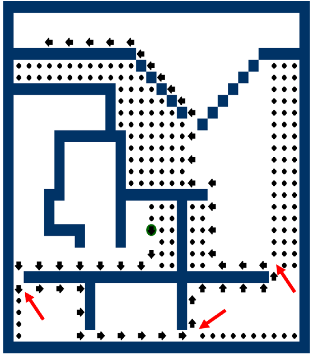
Figure 4: A snapshot from an example run of FCDFS. $s$ is the green circle, black arrows are active robots, black “dots” are settled robots, the blue region is $R^{c}$ and the white region is $R$. The primary direction of each robot is indicated by the direction the arrow representing it is facing. Red arrows point to some of the halls.

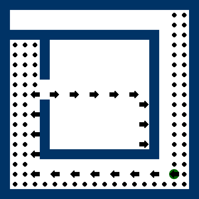
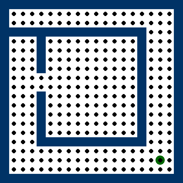
Figure 5: Snapshots from a simulation of FCDFS. Rather than block active robots, the settled robots form halls to enable the swarm to explore more of the environment.

As in Proposition III.3, let $R(t)$ be the initial environment $R$ after removing every vertex that is occupied by a settled robot at time $t$. A robot running FCDFS at time $t$ is searching for the corners and halls of $R(t)$. However, since we assume no communication capabilities, robots are unable to distinguish between active robots, and walls or settled robots. Hence, it is important to design FCDFS so that a robot never misidentifies a corner of $R(t)$ as a hall due to an active robot (rather than a wall or a settled robot) occupying the diagonal and being identified as an obstacle. For this purpose we enable our robots to remember their two previous locations. We will show that an active robot can occupy the diagonal of a corner at time $t$ if and only if its predecessor occupied this diagonal at time $t-2$, thereby allowing the predecessor to distinguish between ’real’ and ’fake’ halls.

Pseudo-code for FCDFS is given in Algorithm 1. The code outlines the Compute step of the Look-Compute-Move cycle. Note that since our robots operate in Look-Compute-Move cycles, when the pseudocode says “step,” we mean that this is the step the robot will take during the Move phase, and not a movement that occurs during computation. In Algorithm 1, we denote by $prev(A)$ the position of a robot $A$ at the beginning of the previous time step, and by $next(A)$ its position at the beginning of the next time step. Section -B shows how FCDFS can be implemented using $5$ bits of persistent state memory (see Algorithm 3).

Algorithm 1 Find-Corner Depth-First Search (local rule for active robots)

Let $v$ be the current location of $A$.

if all neighboring vertices of $v$ are occupied then

     Settle.

else if $A$ has never moved then$\triangleright$ Initialization

     Search clockwise, starting from the ”up” direction, for an unoccupied vertex, and set primary direction to point to that vertex.

end if

if $A$ can move in its primary direction then

     Step in the primary direction.

else if $A$ can step in secondary direction then

     Step in the secondary direction.

else$\triangleright$ We are at a corner or a hall.

     if Three neighboring vertices of $v$ are occupied then

         Settle.$\triangleright$ Corner with three walls.

     else if $prev(prev(A))=diag(v)$ or $diag(v)$ is unoccupied then

         Settle.

     else$\triangleright$ We think we are at a hall.

         Set primary direction to point to the neighbour of $v$ different from $prev(A)$.

         Move in the primary direction.

     end if

end if

IV-A Analysis

In this section we analyze the FCDFS algorithm and prove its optimality.

Lemma IV.5.

Let $c$ be a corner of a simply connected region $R$. Then:

1. $R-c$ (the region $R$ after removing $c$) is simply connected.

2. For any two vertices $u,v$ in $R-c$, the distance between $u$ and $v$ is the same as in $R$.

Proof.

Removing $c$ does not affect connectedness, nor does it affect the distance from $u$ to $v$, as any path going through $c$ can instead go through $diag(c)$. Further, as $c$ is adjacent to two walls, no path in $R-c$ can surround it, so $R-c$ also remains simply connected. ∎

An articulation point (also known as a separation or cut vertex) is a vertex of a graph whose deletion increases the number of connected components of the graph (i.e. disconnects the graph) [42].

Lemma IV.6.

The halls of a simply connected region are articulation points.

Proof.

Let $h$ be a hall of a simply connected region $R$. Suppose for contradiction that $h$ is not an articulation point, and let $u$ and $u^{\prime}$ be the neighbours of $h$. Then there is a path from $u$ to $u^{\prime}$ that does not pass through $h$. Let $P$ be this path, and let $P^{\prime}$ be the path from $u$ to $u^{\prime}$ that goes through $h$.

When embedded in the plane in the usual way, $R$ is in particular a simply connected topological space. The hall $h$ is embedded onto a unit square, whose four corners each touch a wall: three touch the two walls adjacent to $h$, and the fourth touches $diag(h)$. Joined together to form a closed curve, the paths $P$ and $P^{\prime}$ form a rectilinear polygon that must contain at least one corner of $h$ in its interior. Hence, the curve $PP^{\prime}$ in $R$ contains a part of $R^{c}$. This is a contradiction to the assumption that $R$ is simply connected, as it implies $R^{c}$ has at least two disconnected components. (See Figure 6).∎

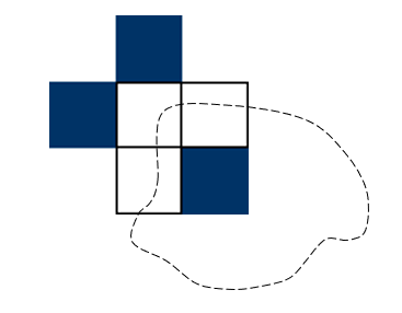
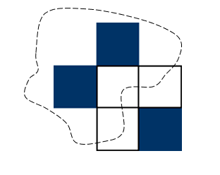
Figure 6: The two possibilities for $PP^{\prime}$.

Lemma IV.6 indicates that $R$ can be decomposed into a tree structure $T(R)$ as follows: first, partition $R$ into the distinct connected components $C_{1},C_{2},\ldots,C_{m}$ that result from the deletion of all halls. Letting the vertices of $T(R)$ each represent one of these components, connect $C_{i}$ and $C_{j}$ by an edge if they are both adjacent to the same hall in $R$. We set $C_{1}$ to be the root of the tree, and to be the connected component containing the door vertex $s$.

By Lemma IV.5, assuming our robots correctly stop only at corners, $R(t)$ can in the same manner be decomposed into a tree $T(R(t))$ whose vertices represent connected components $C_{1}(t),C_{2}(t),\ldots$. These components are each a sub-region of some connected component $C_{i}$ of $R$.

In the next several propositions, we make the no fake halls at time $t$ assumption. This is the assumption that for any $t^{\prime}<t$, at the end of time step $t^{\prime}$: robots can only become settled at corners of $R(t^{\prime})$, and can only change primary directions at halls of $R(t^{\prime})$. We will later show that the “no fake halls” assumption is always true, so the propositions below hold unconditionally.

Proposition IV.7.

Assuming no fake halls at time $t$, a robot $A_{i}$ active at the beginning of time step $t$ has traveled an optimal path in $R$ from $s$ to its current position.

Proof.

By the assumption, the only robots that became settled did so at corners. Consequently, by Lemma IV.5, $R(t)$ is a connected graph, and there is a path in $R(t)$ from $s$ to $A_{i}$. The path $A_{i}$ took might not be in $R(t)$, but whatever articulation points (and in particular halls) $A_{i}$ passed through must still exist, by definition.

Since $A_{i}$ is active at the beginning of time $t$, by the algorithm, it has taken a step every unit of time up to $t$. Until $A_{i}$ enters its first hall, and between any two halls $A_{i}$ passes through, it only moves in its primary and secondary directions. This implies that the path $A_{i}$ takes between the halls of $R(t)$ must be optimal (since it is optimal when embedded onto the integer grid $\mathbb{Z}^{2}$). We note also that $A_{i}$ never returns to a hall $h$ it entered a connected component of $R(t)$ from, since the (possibly updated) primary direction pulls it away from $h$.

We conclude that $A_{i}$’s path consists of taking locally optimal paths to traverse the connected components of the tree $T(R(t))$ in order of increasing depth. Since in a tree there is only one path between the root and any vertex, this implies that $A_{i}$’s path to its current location is at least as good as the optimal path in $R(t)$. By Lemma IV.5, b, this implies that $A_{i}$’s path is optimal in $R$. ∎

Corollary IV.8.

Assuming no fake halls at time $t$,

1. For all $i<j$, the distance between the robots $A_{i}$ and $A_{j}$, if they are both active at the beginning of $t$, is at least $2(j-i)$

2. No collisions (two robots occupying the same vertex) have occurred.

Proof.

For proof of (a), note that at least two units of time pass between every arrival of a new robot (since in the first time step after its arrival, a newly-arrived robot blocks $s$). Hence, when $A_{j}$ arrives, $A_{i}$ will have walked an optimal path towards its eventual location at time $t$, and it will be at a distance of $2(j-i)$ from $s$. This distance is never shortened up to time $t$, as $A_{i}$ will keep taking a shortest path.

(b) follows immediately from (a). ∎

Using Corollary IV.8 it is straightforward to show:

Lemma IV.9.

Suppose $A_{i}$ is active at the beginning of time step $t$. Assuming no fake halls at time $t$, $next(A_{i+1})=prev(A_{i})$.

Lemma IV.9 also implies that if $A_{i}$ is active at the beginning of time step $t$, then $A_{i+1}$ will be active at the beginning of time step $t+1$.

We can now show that the “no fake halls” assumption is true, and consequently, the propositions above hold unconditionally.

Proposition IV.10.

For any $t$, at the end of time step $t$: robots only become settled at corners of $R(t)$, and only change primary directions halls of $R(t)$ (not including the primary direction decided at initialization).

Proof.

The proof of the proposition is by induction. The base case for $t=1$ is trivially true.

Suppose that up to time $t-1$, the proposition holds. Note that this means the “no fake halls” assumption holds up to time $t$, so we can apply the lemmas and propositions above to the algorithm’s configuration at the beginning of time $t$.

We will show that the proposition statement also holds at time $t$. Let $A_{i}$ be an active robot whose location at the beginning of $t$ is $v$. First, consider the case where $v=s$. The algorithm only enables $A_{i}$ to settle at $s$ if it is surrounded by obstacles at all directions. Any obstacle adjacent to $A_{i}$ must be a wall of $R(t)$ (as any active robot must be at a distance at least $2$ from $A_{i}$, due to Corollary IV.8). Hence, if $A_{i}$ settles at $s$, $s$ is necessarily a corner, as claimed.

We now assume that $v\neq s$. We separate the proof into two cases:

Case 1: Suppose $A_{i}$ becomes settled at the end of time step $t$. Then by the algorithm, at the beginning of $t$, $A_{i}$ detects obstacles in its primary and secondary directions. These must be walls of $R(t)$ due to Corollary IV.8, so $v$ is either a corner or a hall of $R(t)$. If three neighbors of $v$ are occupied then $v$ is a corner. Otherwise, since $A_{i}$ settled, we further know that either $diag(v)$ is empty, or $prev(prev(A_{i}))=diag(v)$. In the former case, $v$ is a corner of $R(t)$. In the latter case, we know from Lemma IV.9 and from the fact that no collisions occur that the only obstacle detected at $diag(v)$ is $A_{i+1}$, which is an active robot, so $v$ is again a corner of $R(t)$. In either case a corner is detected and the agent is settled.

Case 2: Suppose $A_{i}$ changed directions at the end of time step $t$. Then it sees two adjacent obstacles, and an obstacle at $diag(v)$. As in case 1, we infer that $v$ is either a corner or a hall. If it is a corner, then $diag(v)$ is an active agent. By Corollary IV.8, it is either $A_{i+1}$ or $A_{i-1}$. It cannot be $A_{i+1}$, as then $A_{i}$’s position two time steps ago would have been $diag(v)$, so it would become settled instead of changing directions. It cannot be $A_{i-1}$, as $diag(v)$ is at least as close to $s$ as $v$ is, and $A_{i-1}$ has arrived earlier than $A_{i}$, and has been taking a shortest path to its destination. Hence, $diag(v)$ cannot be an active agent, and $v$ must be a hall as claimed. ∎

We have shown that the no fake halls assumption is justified at all times $t$, hence we can assume that the propositions introduced in this section hold unconditionally.

Proposition IV.11.

Let $V$ be the number of vertices of $R$. At the end of time step $2n$, every cell is occupied by a settled robot.

Proof.

Propositions IV.7 and IV.10 imply that robots take a shortest path in $R$ to their destination. That means that as long as the destination of a robot is not $s$ itself, robots will step away from $s$ one unit of time after they arrive. Until then, this means that robots arrive at $s$ at rate one per two time steps.

Every robot’s end-destination is a corner, and by the initialization phase of the algorithm, the destination is never $s$ unless $s$ is completely surrounded. Since there are no collisions, there can be at most $n$ robots in $R$ at any given time. By Lemma IV.5, robots that stop at corners keep $R$ connected. Furthermore, every $R(t)$ is a rectilinear polygon, so unless it has exactly one vertex, it necessarily has at least two corners. This means that the destination of every robot is different from $s$ unless $s$ is the only unoccupied vertex. Hence, a robot whose destination is $s$ will only arrive when $s$ is the only unoccupied vertex, and this will happen when $n$ robots have arrived, that is, after at most $2n-1$ time steps. After another time step, this robot settles, giving us a makespan of $2n$. This is exact, since it is impossible to do better than $2n$ makespan. ∎

Propositions IV.11 and IV.7, alongside the “no fake halls” proof, complete our analysis. They show that FCDFS has an optimal makespan of $\mathcal{M}=\mathcal{M}^{*}=2n$, and also that $E_{max}=E_{max}^{*}=1+\max_{v\in R}{\textrm{dist}(s,v)}$ and $E_{total}=E_{total}^{*}=n+\sum_{v\in R}{\textrm{dist}(s,v)}$, since every robot travels a shortest path to its destination without stopping. By the same reasoning, $T_{max}=T_{max}^{*}=\max_{v\in R}{\textrm{dist}(s,v)}$ and $T_{total}=T_{total}^{*}=\sum_{v\in R}{\textrm{dist}(s,v)}$.

In practice, the energy savings of FCDFS are dependent on the shape of the environment $R$. We take as a point of comparison the Depth-First Leader-Follower algorithm of Hsiang et al. [3], described in Proposition III.4. On a 1-dimensional path environment of length $n$, both FCDFS and DFLF require the same total travel, $\mathcal{O}(n^{2})$, so no improvement is attained. In contrast, on an $n$-by-$n$ square grid, DFLF requires total travel $\mathcal{O}(n^{4})$ in the worst case, and FCDFS requires $\mathcal{O}(n^{3})$ - significantly less. This is because the DFLF strategy starting from a corner might cause the leader, $A_{1}$, to “spiral” inwards into the grid, covering every one of its $n^{2}$ vertices in $n^{2}-1$ moves. The robot $A_{i}$ will then make $n^{2}-i$ moves, for a sum total of $O(n^{4})$. FCDFS, on the other hand, distributes the path lengths more uniformly. More environments are compared in Section VI. Note that both algorithms take the exact same amount of time to finish.

Where is it best to place $s$? If we want to minimize the total travel, by the formula given above, the best place to place $s$ is the vertex of $R$ that minimizes the sum of distances $\sum_{v\in R}{\textrm{dist}(s,v)}$ (there may be several). This is the discrete analogue of the so-called Fermat-Toricelli point, or the “geometric median” [43].

IV-B Alternate Optimal Strategies

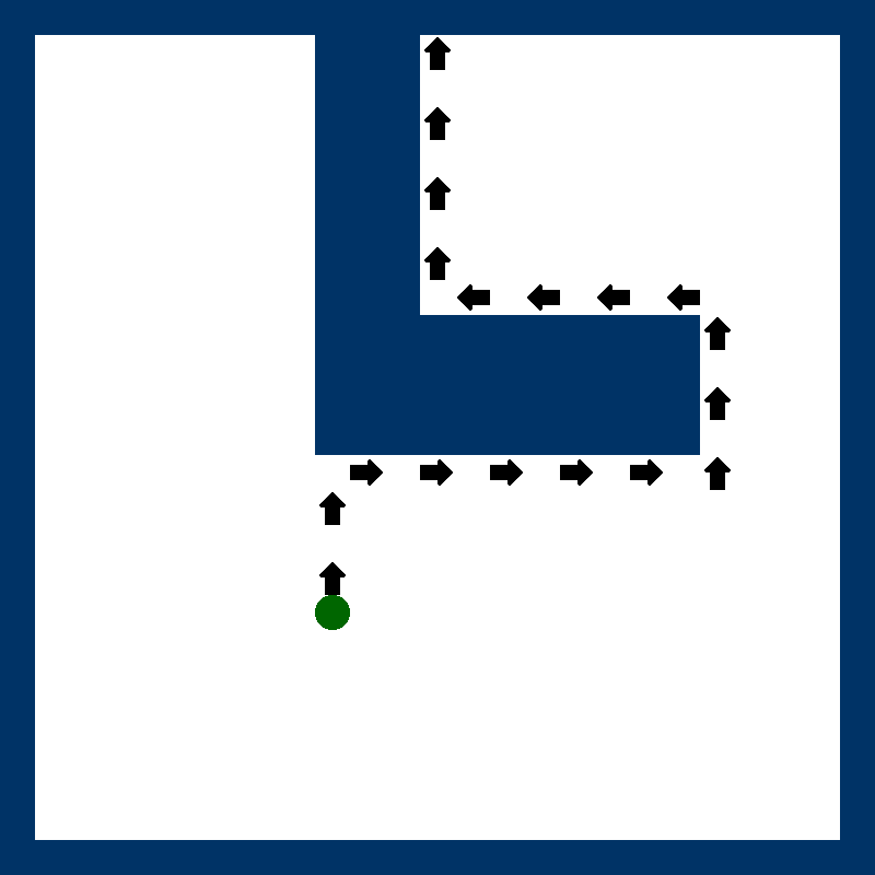
Figure 7: Robots navigate according to “left hand on wall” until a corner is found.

The key idea of FCDFS to maintain a “geometric invariant”: the environment must remain simply connected after a robot settles. As long as this invariant is maintained, the underlying details of the algorithm can vary. For example, a possible variant of FCDFS that is similarly time- and energy-optimal is shown in Figure 7 (analysis omitted). Rather than stick to their secondary and primary directions, robots move using a “left hand on wall” rule until they hit a corner or a wall.

V Asynchronous FCDFS

In real-world multi-robot systems, each autonomous robot activates asynchronously, independent of other robots. One way to introduce asynchronicity into our system is to assume that at every time step, each robot has only a probability $p$ of waking up. When a robot wakes up, it performs the same Look-Compute-Move cycle as before. The source vertex $s$ wakes up at every time step with probability $p$, and upon wake-up inserts a robot into $R$, assuming no robot is currently located at $s$. Since we assume our robots communicate by light, sound, or other local physical signals, we assume that the last message broadcast by a robot $A_{i}$ continues to be broadcast in subsequent time steps, until $A_{i}$ broadcasts a new message. In other words, we assume that as long as $A_{i}$ is active, it continuously broadcasts its last message. This is akin to $A_{i}$ turning on a light or continuously emitting a sound.

These modifications, leaving everything else in our model the same (Section II), result in an asynchronous model of swarms with local signalling. We wish to find a version of FCDFS that works in this asynchronous setting, and to study its performance. FCDFS as implemented in Algorithm 1 relies crucially on the synchronous time scheme to identify halls. This is primarily because, assuming $0$ bits of communication bandwidth, robots in our model cannot tell the difference between obstacles (or settled robots) and active robots. In an asynchronous time scheme, the inability to recognize active robots can also cause robots to split away from the trail of robots that tends forms under FCDFS (see Figure 4). Both these issues can be fixed by enabling the robot executing FCDFS to detect active robots. This can be done by giving robots a single bit of communication bandwidth ($B=1$) and having them broadcast ‘$1$’ as long as they are active, indicating that they are active robots (in fact, this requires “less” than a bit of memory, since the robots never need to broadcast ‘$0$’). Note that, strictly speaking, such robots are no longer ant-like, but they still have very low capability requirements.

An asynchronous version of FCDFS incorporating the above idea is outlined in Algorithm 2. We call this version “AsynchFCDFS” and it is a $(2,1,5)$-algorithm.

Algorithm 2 Asynchronous Find-Corner Depth-First Search (local rule for active robots)

Broadcast “1”.$\triangleright$ Inform other robots that you are active.

Let $v$ be the current location of $A$.

Let $v_{primary}$ be the closest vertex in the primary direction of $A$.

Let $v_{secondary}$ be the closest vertex in the secondary direction of $A$.

if all neighbouring vertices of $v$ contain obstacles that are not robots broadcasting “1” then

     Settle.

else if $A$ has never moved then$\triangleright$ Initialization

     if a neighbor of $v$ contains a robot broadcasting “1” then

         Do nothing this time step.$\triangleright$ Wait until active robots move away.

     else

         Search clockwise, starting from the ”up” direction, for an unoccupied vertex and set primary direction to point to that vertex.

     end if

end if

if $v_{primary}$ contains a robot broadcasting “1” then

     Do nothing this time step.

else if $v_{primary}$ is empty then

     Step in the primary direction.

else if $v_{secondary}$ contains a robot broadcasting “1” then

     Do nothing this time step.

else if $v_{secondary}$ is empty then

     Step in the secondary direction.

else$\triangleright$ We are at a corner or a hall.

     if Three neighboring vertices of $v$ contain walls or settled robots then

         Settle.$\triangleright$ Corner with three walls.

     else if $diag(v)$ is unoccupied or contains a robot broadcasting “1” then

         Settle.

     else$\triangleright$ We think we are at a hall.

         Set primary direction to point to the neighbour of $v$ different from $prev(A)$.

         Move in the primary direction.

     end if

end if

Essentially, Algorithm 2 causes every robot to follow the same path it would under regular FCDFS, by requiring that it wait in place if an active robot is occupying the direction it wants to step in, until that active robot frees up space. This immediately tells us that Algorithm 2 is $T_{total}$ and $T_{max}$-optimal. Our main goal is thus to analyze the energy and makespan cost of the “pauses”. Since our robots’ activation times are now drawn from a random distribution, we will bound these costs probabilistically.

Studying the interactions of independently activating autonomous particles (in this case, modelling our robots) is generally considered a difficult and technical problem. Our key strategy is to side-step the difficulties of analyzing these interactions from scratch by relating a swarm of robots executing AsynchFCDFS to the “Totally Asymmetric Simple Exclusion Process” (TASEP) in statistical physics. Our high level strategy is to use coupling to show that, in the worst case, AsynchFCDFS behaves similar to what is referred to as TASEP with step initial conditions, which is nowadays well-understood [22, 23, 38, 37, 24]. The main idea for this approach comes from [7], in which the makespan of a different (“dual-layered”) uniform dispersion algorithm is studied using similar techniques. We generalize the techniques of [7] to study makespan and energy in our setting.

Define the constant $\alpha=\frac{1}{2}(1-\sqrt{1-p})$. We show the following bound on makespan:

Proposition V.1.

The makespan of AsynchFCDFS over any region $R$ with $n$ vertices fulfills $\mathcal{M}\leq(\frac{1}{\alpha}+o(1))n$ asymptotically almost surely for $n\to\infty$ (i.e., with probability converging to $1$ as $n$ grows to infinity).

Setting $p=1$ gives $\mathcal{M}=(2+o(1))n$, asymptotically matching the synchronous case. Regarding energy consumption, we are able to show:

Proposition V.2.

In an execution of AsynchFCDFS over any region $R$ with $n$ vertices, $E_{max}\leq 2(\frac{1}{\alpha}+o(1))\max_{v\in R}{\textrm{dist}(s,v)}$ asymptotically almost surely for $n\to\infty$.

We shall also pose the following conjecture, based on a heuristic argument and numerical simulations:

Conjecture V.3.

In an execution of AsynchFCDFS over any region $R$ with $n$ vertices, $E_{total}\leq(\frac{c}{\alpha}+o(1))\sum_{i=1}^{n}{\textrm{dist}(s,v_{i})}$ asymptotically almost surely for $n\to\infty$ and some constant $c>0$.

Since $p/\alpha\leq 4$ and $\mathcal{M}$ is bounded below by $n/(p-o(1))$ asymptotically almost surely (as robots are inserted at rate $p$), Proposition V.1 indicates that AsynchFCDFS’s makespan is asymptotically within a constant factor of optimal performance. Similarly, $E_{max}\geq\frac{1}{p-o(1)}\max_{v\in R}{\textrm{dist}(s,v)}$ a.a.s. (since robots move at rate $p$), so Proposition V.2 implies AsynchFCDFS is asymptotically within a constant factor of optimal maximal individual energy use. V.3 hypothesizes the same is true regarding total energy use. Hence, we believe AsynchFCDFS to be highly energy- and makespan-efficient in asynchronous settings, just as FCDFS is in synchronous settings.

V-A Analysis

The execution of (synchronous) FCDFS over a region of interest $R$ is deterministic, and so we know in advance the path each robot shall take. Let us define a graph, $G(R)$, whose nodes are the locations of $R$ and where there is an edge between two locations $v_{i},v_{j}$ if at some point a robot moves from $v_{i}$ to $v_{j}$ during an execution of FCDFS. Recalling our analysis of FCDFS, it is not difficult to prove that $G(R)$ is a tree. Although robot wake-up times are random in our asynchronous model, the ultimate path each robot follows according to AsynchFCDFS is deterministic - it is the same path that robot would follow under FCDFS. Hence, in AsynchFCDFS, too, each robot moves down the edges of the tree $G(R)$.

To study the makespan of AsynchFCDFS, we use coupling, drawing on a technique from [7]. Suppose that there is an infinite collection of agents $A_{1},A_{2},\ldots A_{\infty}$, such that each agent $A_{i}$ wakes up with probability $p$ at every time step $t=0,1,\ldots$. We can associate with every agent $A_{i}$ a list of the times it wakes up, called $\mathcal{S}_{i}$. Suppose further that we execute FCDFS over different regions, say $R$ and $R^{\prime}$. Let $A_{i}^{R}$ and $A_{i}^{R^{\prime}}$ be the $i$th agents to enter $R$ and $R^{\prime}$ respectively. We couple $A_{i}^{R}$ and $A_{i}^{R^{\prime}}$ by assuming that both $A_{i}^{R}$ and $A_{i}^{R^{\prime}}$’s wake-up times are determined by $\mathcal{S}_{i}$. For formal purposes, when $A_{i}^{R}$ or $A_{i}^{R^{\prime}}$ are not yet inside $R$, we still consider them to “wake up” at time steps $t\in\mathcal{S}_{i}$. This is a purely “virtual” wake-up: such robots do and affect nothing upon wake-up. The source vertices of $R$ and $R^{\prime}$ can similarly be coupled.

Let $P_{n}$ be a “straight path” region consisting of the vertices $\{p_{i}\mid 0\leq i<n\}$ where $p_{i}=(i,0)$ and the source, $s$, is located at $p_{0}$. Furthermore, consider the stochastic process called TASEP with step initial conditions [24], which consists of an infinite path region $P(\infty)=\{p_{i}\mid i\in(-\infty,\infty)\}$, where there is no source $s$ but instead the agent $A_{i}$ is initially located at $p_{-i}$. Finally, let $R$ be any region of interest consisting of $n$ vertices. To study the asymptotic performance of FCDFS over $R$, we shall couple the agents over TASEP, $P_{n}$ and $R$ (see Figure 8). Let us denote by $A_{i}^{\mathrm{TASEP}}$, $A_{i}^{P(n)}$, $A_{i}^{R}$, the $i$th agent in each of these coupled processes, respectively.

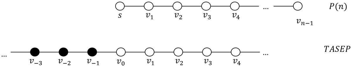
Figure 8: Illustration of $P(n)$ and TASEP with step initial conditions. Black vertices contain agents. Note that TASEP is infinite and lacks a source vertex.

We require a notion of the distance an agent has travelled on $R$ and $P(n)$:

Definition V.4.

The depth at time $t$ of an agent $A_{i}^{R}$ executing FCDFS over a region $R$, denoted $depth_{i}^{R}(t)$, is the number of times $A_{i}$ has moved before time $t$. $depth_{i}^{R}(t)=-1$ if $A_{i}$ has not entered $R$ by time $t$, and $0$ at time of entry. We similarly define $depth_{i}^{P(n)}(t)$.

Note that any robot that increases its depth is moving down the tree $G(R)$ from its current location $v\in G(R)$ to one of $v$’s descendants. Let us prove the following statement:

Lemma V.5.

If the agent $A_{i}^{R}$ is not settled at time $t$ then:

1. $A_{i}^{P(n)}$ is not settled at time $t$, and

2. $depth_{i}^{R}(t)\geq depth_{i}^{P(n)}(t)$.

Proof.

We prove this lemma by induction over $t$. At $t=0$, statements (1) and (2) are vacuously true. Now suppose we are at time $t+1$, and statements (1) and (2) hold at time $t$. Suppose for contradiction that statements (1) or (2) don’t hold at time $t+1$. This means there exists $i$ such that $A_{i}^{R}$ is not settled at time $t+1$ and either (a) $A_{i}^{P(n)}$ is settled at time $t+1$, or (b) $depth_{i}^{R}(t+1)<depth_{i}^{P(n)}(t+1)$.

Assume first, for contradiction, that (a) is true and (b) is not true. By the structure of $P(n)$, $A_{i}^{P(n)}$ being settled means that $depth_{i}^{P(n)}(t)=n-i-1$ and that (if $i>1$) all of $v_{n-i},\ldots v_{n-1}$ contain the settled robots $A_{1}^{P(n)},\ldots A_{i-1}^{P(n)}$ at time $t$. By (1) and (2), this means that $A_{1}^{R},\ldots A_{i-1}^{R}$ are settled at time $t$. Since $A_{i}^{R}$ is not settled at time $t+1$, this must mean that either it moved and increased its depth since time $t$, or it was adjacent a active agent in one of its primary directions at time $t$. The latter is impossible, since (by the FCDFS algorithm) such an agent must have been one of the agents $A_{1}^{R},\ldots A_{i-1}^{R}$. Hence, $A_{i}^{R}$ must have moved at time $t$. By our assumptions, this implies $depth_{i}^{R}(t+1)\geq depth_{i}^{P(n)}(t)+1=n-i$. But this is impossible, since there are at least $i-1$ settled agents in $R$ at time $t+1$, hence the maximum depth an active agent can have is $n-i-1$. Contradiction.

Next, let us assume for contradiction that (b) is true. By the inductive assumption, this implies that $depth_{i}^{P(n)}(t)=depth_{i}^{R}(t)$ and $depth_{i}^{P(n)}(t+1)=depth_{i}^{R}(t+1)+1$, which can only occur if $A_{i}^{P(n)}$ moves at time $t$ and $A_{i}^{R}$ does not. $A_{i}^{R}$ not moving at time $t$ implies (due to the fact it is moving along the edges of the tree $G(R)$) that there is some $j<i$ such that $depth_{j}^{R}(t)=depth_{i}^{R}(t)+1$. Since $A_{i}^{P(n)}$ does move at time $t$, by the structure of $P(n)$ we infer that $depth_{j}^{P(n)}(t)>depth_{i}^{P(n)}(t)+1$. However, again by (2), at time $t$ we have $depth_{j}^{R}(t)\geq depth_{j}^{P(n)}(t)$, which implies $depth_{j}^{R}(t)>depth_{i}^{P(n)}(t)+1=depth_{i}^{R}(t)+1$. Contradiction. ∎

Let $x_{i}(t)$ be the $x$ coordinate of $A_{i}^{\mathrm{TASEP}}$’s location at time $t$ (where the $x$ coordinate of $v_{i}\in P(\infty)$ is $i$). It is straightforward, using coupling and induction as in Lemma V.5, to show that:

Lemma V.6.

If the agent $A_{i}^{P(n)}$ is not settled at time $t$ then $depth_{i}^{P(n)}(t)\geq x_{i}(t)$.

Lemma V.6 can also be rephrased as: if $depth_{i}^{P(n)}(t)<x_{i}(t)$ then $A_{i}^{P(n)}$ is settled. As a corollary, we infer:

Corollary V.7.

If at least $n+1$ TASEP agents have non-negative $x$ coordinate at time $t_{0}$ then the makespan of FCDFS over $R$ obeys $\mathcal{M}\leq t_{0}$.

Note that here we are referring to the makespan of FCDFS over $R$ in given an arbitrary list of wake-up times. The list of wake-up times is randomly distributed (and so is $\mathcal{M}$), but Corollary V.7 is true for any such list.

Proof.

Suppose for contradiction that some agent $A_{i}^{R}$, $1\leq i\leq n$, is not settled, but the $n+1$ agents $A_{1}^{\mathrm{TASEP}},\ldots A_{n}^{\mathrm{TASEP}}$ have non-negative $x$ coordinate. By Lemma V.5 we infer that $A_{i}^{P(n)}$ is not settled, and by Lemma V.5 we infer $depth_{i}^{P(n)}(t)\geq x_{i}(t)$. However, the maximum possible depth of $A_{i}^{P(n)}$ is $n-i$, whereas $x_{i}(t)$ is at least $n-i+1$, since at least $n-i+1$ agents are located to its left and to the right of $v_{0}$. Contradiction. ∎

We can now prove Proposition V.1. We use a similar idea as Lemma III. 14 of [7].

Proof of Proposition V.1.

Let $F(t)$ denote the number of agents in TASEP that have non-negative $x$ coordinate at time $t$. It is known (see, e.g., [24, 40]) that $F(t)$ fulfills:

$$\lim_{t\to\infty}\mathbb{P}(F(t)-\alpha t\leq Vt^{1/3}s)=1-TW_{2}(-s)$$ (1)

where $V=2^{-4/3}p^{1/3}(1-p)^{1/6}$ and $TW_{2}(-s)$ is the Tracy-Widom distribution. $TW_{2}(-s)$ obeys the asymptotics $TW_{2}(-s)=O(e^{-c_{1}s^{3}})$ and $1-TW_{2}(s)=O(e^{-c_{2}s^{3/2}})$ as $s\to\infty$ for some $c_{1},c_{2}>0$.

Let $t_{k}=(1/\alpha+k^{-1/3})k$. We wish to show that $\mathcal{M}\leq t_{n+1}$ asymptotically almost surely as $n\to\infty$. By Corollary V.7, this is equivalent to showing that $X_{n}=\mathbb{P}(F(t_{n})<n)$ tends to $0$ as $n\to\infty$ (because the probability that $\mathcal{M}\leq t$ is at least $1-X_{n+1}$). Define the probability

$$p(n,s)=\mathbb{P}(F(t_{n})-\alpha t_{n}\leq Vt_{n}^{1/3}s)$$ (2)

$p(n,s)$ is clearly monotonic non-decreasing in $s$. Define $s_{n}=(n-\alpha t_{n})V^{-1}t_{n}^{-1/3}$, yielding $X_{n}=p(n,s_{n})$. For any constant $C$, define $Y_{n}=p(n,C)$. Since $s_{n}$ tends to $-\infty$ as $n\to\infty$, we must have $s_{n}<C$ for sufficiently large $n$, hence $X_{n}\leq Y_{n}$ for sufficiently large $n$. Using Equation 1 and taking $C\to-\infty$ shows that $X_{n}$ tends to $1-TW_{2}(\infty)=0$ as $n\to\infty$, completing the proof. ∎

The proof of Proposition V.2 uses a similar technique to that of Proposition V.1, so we omit some repetitive details and focus on the new ideas:

Proof sketch of Proposition V.2.

Let $d=\max_{v\in R}{\textrm{dist}(s,v)}$. Consider the execution of AsynchFCDFS over some region $R$ with $n$ vertices. The key idea of the proof is that at any given time, there can be no more than $d$ active robots in $R$. This is because all active agents always trace the path of the active agent $A_{i}$ with smallest index $i$ until it settles, and the path of $A_{i}$ is always a shortest path from $s$ to some vertex $v$. This path can contain at most $d$ vertices, and so there can be at most $d$ active agents.

Consider a new agent $A_{j}$ that has emerged from $s$ at time step $t$. Since there can be at most $d$ active agents at a time, $A_{j}$ is necessarily settled once $d$ newer agents have emerged from $s$. The time it takes $d$ agents to emerge after $A_{j}$ is dominated by the time it takes $2d$ agents to emerge in $R(t)$ (we can show this formally by the same type of coupling as Lemma V.5). As we’ve seen in the proof of Proposition V.1, the time it takes $2d$ agents to emerge in $R(t)$ is dominated by the time it takes $2d$ agents to attain non-negative coordinates in TASEP, which we’ve previously shown is asymptotically almost surely less than $2(1/\alpha+o(1))d$ for large values of $d$. We complete the proof by noting that $d$ necessarily tends to $\infty$ as $n\to\infty$. ∎

We believe V.3, which states that $E_{total}$ is within a constant factor of optimal energy use, to be true, because every robot in AsynchFCDFS travels the same optimal path it does in FCDFS, and our results in this section hint that it may move at a linear rate toward this destination (indeed, Proposition V.2 establishes this for robots that travel distance $\max_{v\in R}{\textrm{dist}(s,v)}$). However, we struggled bounding $E_{total}$ with our current approach. The main challenge is that Equation 1 is given as a limit, making it difficult to estimate the energy costs of agents that move short or intermediate distances. We pose this as a question for future work.

VI Empirical Analysis

To verify our theoretical findings, we ran numerical simulations on simply-connected environments of different sizes and obstacle placements. To measure the improvement attained by FCDFS and AsynchFCDFS, we compared it to Hsiang et al.’s DFLF and BFLF algorithms [3]. DFLF is described in Proposition III.4. BFLF (Breadth-First Leader-Follower) is a different makespan-optimal dispersion algorithm that seeks to spread out the agents in a more even way by having multiple leaders, reducing total and maximal individual travel at the cost of energy. Table II summarizes simulation results in two different environments. We see that (as anticipated) the travel for FCDFS and AsynchFCDFS is identical, but makespan and energy use are larger for smaller $p$. Additionally, AsynchFCDFS’s average performance is below (i.e., better than) the bounds of Propositions V.1 and V.2, and V.3 for the tested $p$ values.

Next, we were interested in how FCDFS and AsynchFCDFS’s performance varies as $n$ (the environment size) grows. We plotted the performance of these algorithms alongside DFLF and BFLF on square grids of increasing size: see Figure 9. We see that, although the synchronous algorithms DFLF, BFLF and FCDFS are matched in terms of makespan, FCDFS attains significantly better energy and travel. The asynchronous variant of FCDFS attains worse makespan, as expected (since robots are inactive in some timesteps), but still attains better energy and travel than DFLF and BFLF for $p=0.5,0.75$. AsynchFCDFS’s maximal individual energy use and makespan are below the bounds anticipated by Propositions V.1 and V.2, and total energy use is below the bound anticipated by V.3.

TABLE II: Simulation results over the environments shown in Figures 4 and 5. Each measured performance metric written in the Table is the rounded average of $10$ trials.

Experiment Name	$\boldsymbol{T_{\textbf{total}}}$	$\boldsymbol{T_{\textbf{max}}}$	$\boldsymbol{E_{\textbf{total}}}$	$\boldsymbol{E_{\textbf{max}}}$	$\boldsymbol{\mathcal{M}}$
FCDFS, Fig. 4 Env. ($n=669$)	$35\,103$	$99$	$35\,772$	$100$	$1338$
AsynchFCDFS ($p=0.75$), Fig. 4 Env.	$35\,103$	$99$	$69\,092$	$137$	$2565$
AsynchFCDFS ($p=0.5$), Fig. 4 Env.	$35\,103$	$99$	$118\,658$	$171$	$4350$
BFLF, Fig. 4 Env.	$39\,649$	$117$	$122\,787$	$197$	$1338$
DFLF, Fig. 4 Env.	$91\,959$	$260$	$92\,628$	$261$	$1338$
FCDFS, Fig. 5 Env. ($n=277$)	$5909$	$38$	$6186$	$39$	$554$
AsynchFCDFS ($p=0.75$), Fig. 5 Env.	$5909$	$38$	$11\,783$	$46$	$1027$
AsynchFCDFS ($p=0.5$), Fig. 5 Env.	$5909$	$38$	$20\,001$	$68$	$1725$
BFLF, Fig. 5 Env.	$7313$	$56$	$28\,358$	$130$	$554$
DFLF, Fig. 5 Env.	$17\,214$	$134$	$17\,491$	$135$	$554$

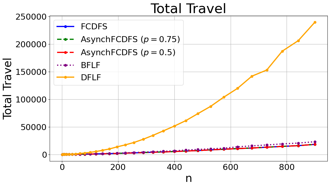
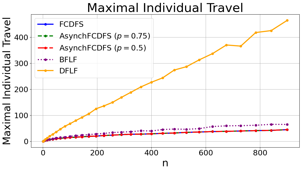
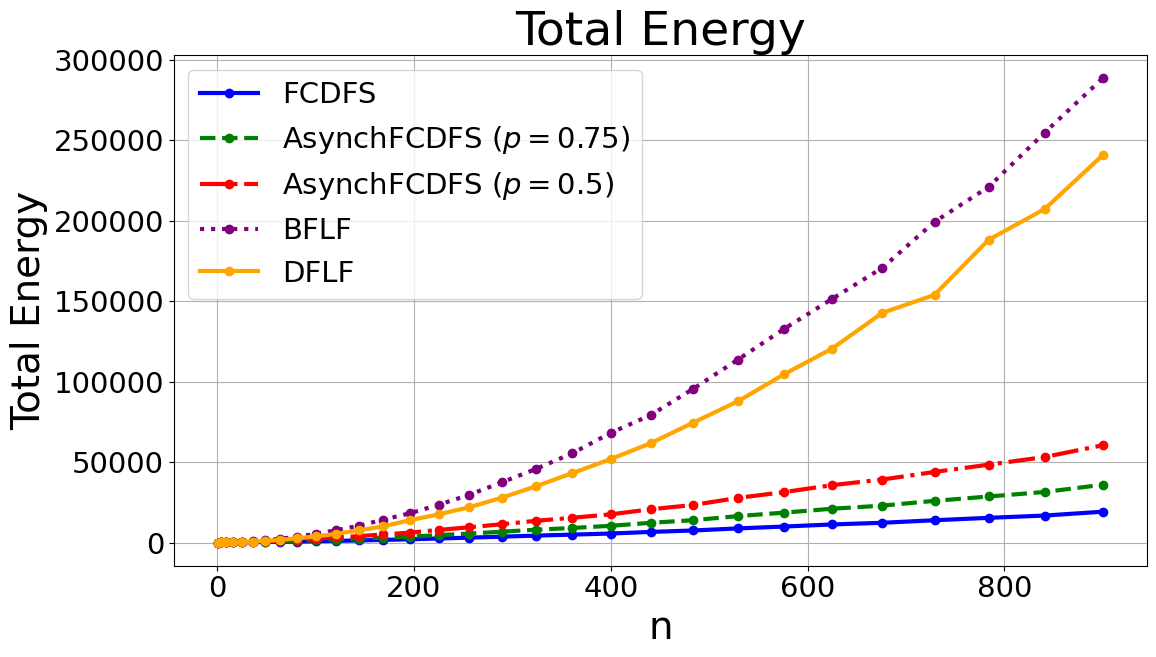
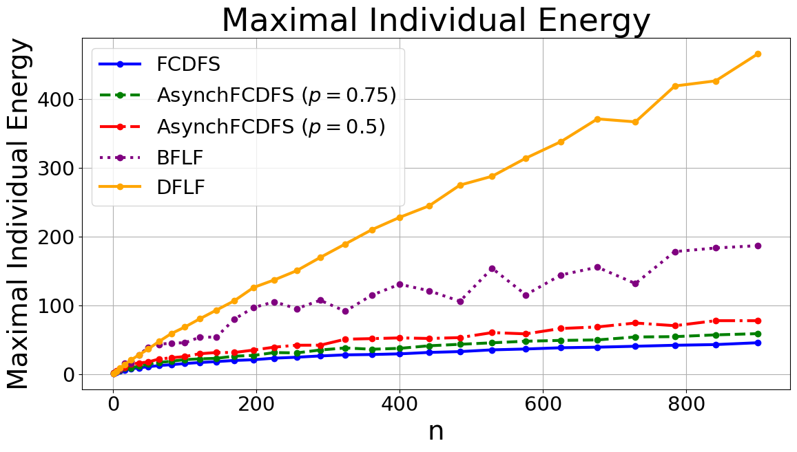
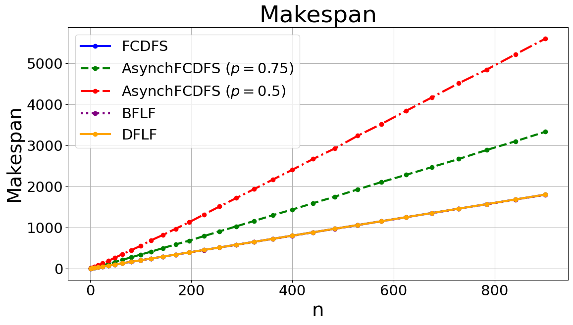
Figure 9: Comparative results of the algorithms across different metrics. For each $k\in[1,30]$, we generated $40$ different square grid environments of size $n=k\times k$ with randomly placed source locations. Each data point is the average of $40$ simulations of its respective algorithm, one per grid environment. In each graph, the $x$ axis is $n$ and the $y$ axis is the performance measure of interest. Note that some algorithms overlap perfectly on metrics such as makespan.

VII Conclusion

This work studied time, travel, and energy use in the uniform dispersion problem. We presented a formal model for comparing swarm algorithms in terms of robot capabilities, and proved that while makespan and travel can be minimized in all environments by swarm robotic algorithms with low capability requirements, energy cannot be minimized even by a centralized algorithm, assuming constant sensing range. In contrast, we showed that energy can be minimized in simply connected environments by an algorithm called FCDFS, executable even by minimal “ant-like” robots with small constant sensing range and memory, and no communication. We extended FCDFS to the asynchronous setting, showing it attains energy consumption within a constant factor of the optimum.

Our results shed light on the relationships between the capabilities of robots, their environment, and the quality of the collective behavior they can achieve. The fact that robots can minimize the travel or makespan even with very limited capabilities, but cannot minimize energy even with arbitrarily strong capabilities, attests to the difficulty of designing energy-efficient collective behaviors. On the other hand, the fact that energy can be minimized by ant-like robots in common types of environments suggests energy efficiency in swarm robotic systems may be practically attainable, especially in restricted settings. Broadly, our results point to the importance of co-design approaches in swarm robotics, carefully tailoring the capabilities of robots to the specific features of the environment they are expected to operate in.

The capability-based modeling approach we presented for uniform dispersion can be applied to other canonical problems in swarm robotics, such as gathering, formation, or path planning. Doing so may reveal additional gaps in capability requirements between robots optimizing different objectives, as well as new co-design opportunities.

References

- [1] E. Şahin, “Swarm robotics: From sources of inspiration to domains of application,” in International workshop on swarm robotics, pp. 10–20, Springer, 2004.
- [2] A. Quattrini Li, “Exploration and mapping with groups of robots: Recent trends,” Current Robotics Reports, vol. 1, no. 4, pp. 227–237, 2020.
- [3] T.-R. Hsiang, E. M. Arkin, M. A. Bender, S. P. Fekete, and J. S. Mitchell, “Algorithms for rapidly dispersing robot swarms in unknown environments,” in Algorithmic Foundations of Robotics V, pp. 77–93, Springer, 2004.
- [4] O. Rappel and J. Ben-Asher, “Area coverage – A swarm based approach,” in 59th Israel Annual Conference on Aerospace Sciences, IACAS 2019, pp. 35–55, Israel Annual Conference on Aerospace Sciences, 2019.
- [5] E. M. Barrameda, S. Das, and N. Santoro, “Uniform dispersal of asynchronous finite-state mobile robots in presence of holes,” in International Symposium on Algorithms and Experiments for Sensor Systems, Wireless Networks and Distributed Robotics, pp. 228–243, Springer, 2013.
- [6] A. Hideg and T. Lukovszki, “Uniform dispersal of robots with minimum visibility range,” in International Symposium on Algorithms and Experiments for Sensor Systems, Wireless Networks and Distributed Robotics, pp. 155–167, Springer, 2017.
- [7] M. Amir and A. M. Bruckstein, “Fast uniform dispersion of a crash-prone swarm.,” Robotics: Science and Systems, 2020.
- [8] O. Rappel, M. Amir, and A. M. Bruckstein, “Stigmergy-based, dual-layer coverage of unknown regions,” in Proceedings of the 2023 International Conference on Autonomous Agents and Multiagent Systems, pp. 1439–1447, 2023.
- [9] E. M. Barrameda, S. Das, and N. Santoro, “Deployment of asynchronous robotic sensors in unknown orthogonal environments,” in International Symposium on Algorithms and Experiments for Sensor Systems, Wireless Networks and Distributed Robotics, pp. 125–140, Springer, 2008.
- [10] E. M. Barrameda, S. Das, and N. Santoro, “Uniform Dispersal of Asynchronous Finite-State Mobile Robots in Presence of Holes,” in Algorithms for Sensor Systems (P. Flocchini, J. Gao, E. Kranakis, and F. Meyer auf der Heide, eds.), vol. 8243, pp. 228–243, Berlin, Heidelberg: Springer Berlin Heidelberg, 2014.
- [11] A. Howard, M. J. Matarić, and G. S. Sukhatme, “An incremental self-deployment algorithm for mobile sensor networks,” Autonomous Robots, vol. 13, no. 2, pp. 113–126, 2002.
- [12] E. D. Demaine, M. Hajiaghayi, H. Mahini, A. S. Sayedi-Roshkhar, S. Oveisgharan, and M. Zadimoghaddam, “Minimizing movement,” ACM Transactions on Algorithms (TALG), vol. 5, no. 3, p. 30, 2009.
- [13] Z. Liao, J. Wang, S. Zhang, J. Cao, and G. Min, “Minimizing movement for target coverage and network connectivity in mobile sensor networks,” network, vol. 4, p. 8, 2015.
- [14] Z. Friggstad and M. R. Salavatipour, “Minimizing movement in mobile facility location problems,” ACM Transactions on Algorithms (TALG), vol. 7, no. 3, p. 28, 2011.
- [15] M. Amir and A. M. Bruckstein, “Minimizing travel in the uniform dispersal problem for robotic sensors,” in Proceedings of the 18th International Conference on Autonomous Agents and MultiAgent Systems, International Foundation for Autonomous Agents and Multiagent Systems, 2019.
- [16] K. D. Joshi, Introduction to general topology. New Age International, 1983.
- [17] A. Shiloni, N. Agmon, and G. A. Kaminka, Of robot ants and elephants. Citeseer, 2010.
- [18] A. Shats, M. Amir, and N. Agmon, “Competitive ant coverage: The value of pursuit,” in 2023 IEEE/RSJ International Conference on Intelligent Robots and Systems (IROS), pp. 6733–6740, IEEE, 2023.
- [19] J.-L. Deneubourg, S. Goss, N. Franks, A. Sendova-Franks, C. Detrain, and L. Chrétien, “The dynamics of collective sorting robot-like ants and ant-like robots,” in From animals to animats: proceedings of the first international conference on simulation of adaptive behavior, pp. 356–365, 1991.
- [20] T. Stirling, S. Wischmann, and D. Floreano, “Energy-efficient indoor search by swarms of simulated flying robots without global information,” Swarm Intelligence, vol. 4, no. 2, pp. 117–143, 2010.
- [21] T. Stirling and D. Floreano, “Energy-Time Efficiency in Aerial Swarm Deployment,” in Distributed Autonomous Robotic Systems (A. Martinoli, F. Mondada, N. Correll, G. Mermoud, M. Egerstedt, M. A. Hsieh, L. E. Parker, and K. Støy, eds.), vol. 83, pp. 5–18, Berlin, Heidelberg: Springer Berlin Heidelberg, 2013.
- [22] M. Prähofer and H. Spohn, “Current fluctuations for the totally asymmetric simple exclusion process,” in In and out of equilibrium, pp. 185–204, Springer, 2002.
- [23] C. A. Tracy and H. Widom, “Asymptotics in asep with step initial condition,” Communications in Mathematical Physics, vol. 290, no. 1, pp. 129–154, 2009.
- [24] K. Johansson, “Shape fluctuations and random matrices,” Communications in Mathematical Physics, vol. 209, pp. 437–476, feb 2000.
- [25] D. Peleg, “Distributed Coordination Algorithms for Mobile Robot Swarms: New Directions and Challenges,” in Distributed Computing – IWDC 2005, pp. 1–12, Springer, Berlin, Heidelberg, Dec. 2005.
- [26] J. Cortes, S. Martinez, T. Karatas, and F. Bullo, “Coverage control for mobile sensing networks,” IEEE Transactions on Robotics and Automation, vol. 20, pp. 243–255, Apr. 2004.
- [27] V. P. Tran, M. A. Garratt, K. Kasmarik, and S. G. Anavatti, “Robust multi-robot coverage of unknown environments using a distributed robot swarm,” arXiv preprint arXiv:2111.14295, 2021.
- [28] V. P. Tran, M. A. Garratt, K. Kasmarik, and S. G. Anavatti, “Dynamic frontier-led swarming: Multi-robot repeated coverage in dynamic environments,” IEEE/CAA Journal of Automatica Sinica, vol. 10, no. 3, pp. 646–661, 2023.
- [29] E. M. Barrameda, S. Das, and N. Santoro, “Deployment of Asynchronous Robotic Sensors in Unknown Orthogonal Environments,” in Algorithmic Aspects of Wireless Sensor Networks (S. P. Fekete, ed.), vol. 5389, pp. 125–140, Berlin, Heidelberg: Springer Berlin Heidelberg, 2008.
- [30] A. Hideg and L. Blázovics, “Area coverage using distributed randomized methods,” in Cybernetics & Informatics (K&I), 2016, pp. 1–5, IEEE, 2016.
- [31] A. Hideg, T. Lukovszki, and B. Forstner, “Improved runtime for the synchronous multi-door filling,” Periodica Polytechnica Electrical Engineering and Computer Science, vol. 66, no. 1, pp. 12–19, 2022.
- [32] Ö. Arslan, “Statistical coverage control of mobile sensor networks,” IEEE Transactions on Robotics, vol. 35, no. 4, pp. 889–908, 2019.
- [33] D. Rabinovich, M. Amir, and A. M. Bruckstein, “Optimally reordering mobile agents on parallel rows,” Theoretical Computer Science, vol. 985, p. 114330, 2024.
- [34] F. Aznar, M. Pujol, R. Rizo, F. A. Pujol, and C. Rizo, “Energy-Efficient Swarm Behavior for Indoor UAV Ad-Hoc Network Deployment,” Symmetry (20738994), vol. 10, p. 632, Nov. 2018. Publisher: MDPI Publishing.
- [35] O. Rappel, J. Ben-Asher, and A. Bruckstein, “Exploration of unknown indoor regions by a swarm of energy-constrained drones,” 05 2023.
- [36] J. Gielis, A. Shankar, and A. Prorok, “A critical review of communications in multi-robot systems,” Current robotics reports, vol. 3, no. 4, pp. 213–225, 2022.
- [37] D. Chowdhury, L. Santen, and A. Schadschneider, “Statistical physics of vehicular traffic and some related systems,” Physics Reports, vol. 329, no. 4-6, pp. 199–329, 2000.
- [38] T. Chou, K. Mallick, and R. Zia, “Non-equilibrium statistical mechanics: from a paradigmatic model to biological transport,” Reports on progress in physics, vol. 74, no. 11, p. 116601, 2011.
- [39] D. Romik, The surprising mathematics of longest increasing subsequences. No. 4, Cambridge University Press, 2015.
- [40] T. Kriecherbauer and J. Krug, “A pedestrian’s view on interacting particle systems, kpz universality and random matrices,” Journal of Physics A: Mathematical and Theoretical, vol. 43, no. 40, p. 403001, 2010.
- [41] M. Amir, D. Rabinovich, and A. M. Bruckstein, “Patrolling grids with a bit of memory,” 2023.
- [42] R. Diestel, Graph Theory (Graduate Texts in Mathematics). Springer, jun 2017.
- [43] J. Krarup and S. Vajda, “On torricelli’s geometrical solution to a problem of fermat,” IMA Journal of Management Mathematics, vol. 8, no. 3, pp. 215–224, 1997.