1 Introduction

Axions and axion-like particles (ALPs, denoted $a$ in the following) are spin-0 particles that are singlets under the Standard Model (SM) gauge groups. ALPs appear in many well-motivated SM extensions, where they arise as pseudo-Nambu-Goldstone bosons of an approximate axion shift-symmetry. As a consequence, the masses of ALPs can naturally be much smaller than the energy scale of the underlying ultraviolet (UV) model, making them an attractive target for the Large Hadron Collider (LHC) and the future High-Luminosity LHC (HL-LHC). While axions have originally been introduced as a potential solution to the strong-CP problem [1, 2, 3, 4], ALPs are featured in a variety of SM extensions [5, 6, 7] including string theory [8, 9], supersymmetric theories [10], dark-matter models [11, 12, 13] and composite Higgs models [14].

Early analyses have focused on generic ALPs with masses below the GeV-range. However, also heavier ALPs with masses of tens or hundreds of GeV that can be resonantly produced at colliders are under active investigation, both in the $pp$ [15, 16, 17, 18] and $\gamma\gamma$ (light-by-light scattering) [19, 20] production channels. In particular, the so-called QCD axion addressing the strong-CP problem can have a mass in the TeV range if its mass receives additional contributions from the confinement scale associated with extra non-abelian gauge groups [21, 22], making it potentially accessible at the LHC [23, 24]. In this context, one should note that such heavy QCD axions are less prone to the so-called axion quality problem [25, 26, 27, 28, 29, 30] of the usual Peccei-Quinn mechanism, such that they are also denoted high-quality axions in recent literature [31]. This further motivates searches for ALPs at the LHC and future accelerators.

In recent studies, limits on ALP couplings arising from existing collider searches have been investigated with a main focus on the ALP couplings to the SM gauge bosons, both for resonant [35, 36, 37, 38, 39, 40] and non-resonant ALP contributions [41, 42, 43, 44, 45]. However, generic ALPs are also expected to be coupled to the SM fermions at the electroweak (EW) scale, e.g. via contributions that are induced by renormalisation-group running even if ALP–fermion couplings are absent in the UV [46, 47, 48, 49]. ALP–fermion couplings are typically assumed to have a flavor-hierarchical structure [50, 51, 52, 53]. Moreover, the couplings of ALPs to fermions are typically proportional to the fermion masses. This results in a particular relevance of the ALP coupling to top quarks. Interactions between the ALP and top quarks are also motivated based on naturalness arguments and (non-minimal) composite Higgs models [14, 54]. Limits on the ALP–top-quark coupling have been derived from $t\bar{t}a$ searches, from the effects of ALPs on ${t\bar{t}}$, ${t\bar{t}}{t\bar{t}}$ and ${t\bar{t}}b\bar{b}$ production [55, 56, 57, 58] as well as from renormalization group (RG) running effects on observables beyond those involving top quarks at the LHC [38]. Constraints from low-energy colliders for ALPs have been derived in Ref. [40]. Moreover, new searches for ALPs at existing [59, 60, 61] and future colliders [62, 63, 64] have been proposed.

In this work (see Ref. [65] for preliminary results), we address ALP contributions to ${t\bar{t}}$ production in the dilepton decay channel for ALPs with masses above the ${t\bar{t}}$ threshold. The possibility to search for new $s$-channel resonances in the $t\bar{t}$ invariant mass distribution at the LHC has been studied in Refs. [66, 67, 68, 69, 70, 71, 72], emphasizing the importance of signal–background interference effects on the shape of the $m_{t\bar{t}}$ distribution and the resulting characteristic “peak-dip” structures. A first search taking into account the interference with the SM background for scalar ${t\bar{t}}$ production has been published by the ATLAS collaboration using $20.3~{}\mathrm{fb}^{-1}$ of 8 TeV $pp$ collisions [73]. Exploring $35.9~{}\mathrm{fb}^{-1}$ of 13 TeV LHC data, the CMS collaboration could further enhance the sensitivity to ${t\bar{t}}$ production via scalar and pseudoscalar resonances [74]. Recently, a preliminary result from ATLAS based on the full Run 2 data set was presented yielding similar expected constraints on the coupling between top quarks and the scalar/pseudoscalar boson [75].

We perform a reinterpretation of the published CMS search for pseudoscalars in terms of ALPs to $t\bar{t}$ production and extend it by considering an ALP with a more general coupling structure which features an additional (besides the contribution induced by the top-quark loop) effective coupling to gluons. Such an additional contribution to the effective gluon coupling could originate, for instance, from heavy vector-like quarks or from colored scalars predicted in Supersymmetry, as studied in Refs. [70, 71]. We address the question how an ALP with both top-quark and gluon couplings could be distinguished from the case where the coupling of the new particle to gluons is induced exclusively through the SM-like top-quark loop. We will refer to the second, more restrictive scenario as a pseudoscalar Higgs boson, denoted as $A$, as it could result from models extending the SM only in the Higgs sector, such as the Two Higgs doublet model (2HDM) [77, 78, 4, 79]. Note that we only use the terms “ALP” and “pseudoscalar Higgs boson” to distinguish between the scenarios with more general and restrictive couplings structures, respectively. In principle, ALPs and pseudoscalar Higgs bosons could feature both coupling structures.

Our analysis is based on the invariant $t\bar{t}$ mass distribution. As our study involves the leptons from the top-quark decay, thereby going beyond the analysis level of stable top quarks as considered, e.g., in Ref. [70, 58], we are able to employ angular variables. Since top quarks decay on timescales shorter than the one of QCD interactions, these variables are sensitive to the $t\bar{t}$ spin correlation which was measured both at the Tevatron $p\bar{p}$ [80] and the LHC $pp$ colliders [81, 82]. Such measurements thus provide additional sensitivity to the presence of new particles above the ${t\bar{t}}$ threshold. The $t\bar{t}$ spin correlation also provides information about the spin and the CP properties of the new particle [83, 68, 84, 69, 70]. Focusing on new spin-0 particles, we consider two benchmark scenarios: (i) a 400 GeV ALP with a relative width of $2.5\%$ and (ii) an 800 GeV ALP with a relative width of $5\%$. Scenario (i) is motivated by a local $3.5\,\sigma$ excess observed by the CMS collaboration in the 400 GeV mass region [74], which has sparked some attention in the literature [85, 86, 87]. No excess at this mass value has been reported in the latest ATLAS result [75]. We will investigate to what extent an ALP with the same mass and width can be distinguished from a pseudoscalar Higgs boson depending on the effective ALP–gluon coupling, even if both particles are produced with the same total cross section. We showcase that the LHC has significant discovery potential for ALPs in this mass range in the near future. Under the assumption that no deviations from the SM expectation will be observed, we set current and projected limits at several stages of the (HL-)LHC program on the ALP couplings to fermions and gluons in terms of the Wilson coefficients of the linear representation of the ALP–SM Lagrangian. Furthermore, we compare these limits to the ones from existing experimental bounds from LHC searches in other final states, most notably from searches for resonances decaying into di-photons [88] and measurements of the production of four top-quarks [89]. We also compare our bounds to other experimental limits, for instance from the study of renormalisation group (RG) running effects that mix ALP Effective Field Theory (EFT) operators and dimension-six Standard Model Effective Field Theory (SMEFT) operators, denoted ALP–SMEFT interference [43, 44].

The paper is organized as follows. In Sect. 2 we introduce the theoretical framework, calculate the partial width of the ALP and describe the Monte Carlo simulation used in our analysis. In Sect. 3 we present our main results, namely ALP bounds from existing searches, the analysis of the sensitivity for distinguishing an ALP from a pseudoscalar Higgs boson, and projected ALP bounds at the LHC, and we compare these to other existing limits. We summarize our results and conclude in Sect. 4.

2 Theoretical framework and event simulation

2.1 The ALP Lagrangian

ALPs are pseudoscalars which preserve the softly broken axion shift symmetry $a(x)\to a(x)+c$, with $c$ being a constant. The general linear ALP–SM Lagrangian at dimension five [51] is given by

$$\mathcal{L}\;=\; \mathcal{L}_{\textrm{SM}}+\frac{1}{2}(\partial_{\mu}a)(\partial^{\mu}a)+\frac{m_{a}^{2}}{2}a^{2}-\frac{a}{f_{a}}c_{G}\,G^{a}_{\mu\nu}\tilde{G}^{a\mu\nu}-\frac{a}{f_{a}}c_{B}\,B_{\mu\nu}\tilde{B}^{\mu\nu}$$

$$-\frac{a}{f_{a}}c_{W}\,W^{I}_{\mu\nu}\tilde{W}^{I\mu\nu}-\frac{\partial^{\mu}a}{f_{a}}\sum_{f}\bar{\Psi}_{f}\mathbf{c}_{f}\gamma_{\mu}\Psi_{f}\,,$$ (1)

where $f_{a}$ and $m_{a}$ denote the ALP decay constant and mass, respectively, and $G$, $W$ and $B$ are the gauge fields associated to the $SU(3)$, $SU(2)$ and $U(1)$ gauge symmetries of the strong and electroweak interactions. The sum in the last term runs over the fermionic fields $f=u_{R},d_{R},Q_{L},L_{L},e_{R}$. In principle, the $\mathbf{c}_{f}$ are $3\times 3$ matrices in flavor space, but we neglect flavor mixing in the following. The invariance of the ALP couplings under the transformation $a\to a+c$ is manifest in the couplings of the ALP to fermions, which are expressed in terms of the derivative of $a$. Additional operators arise from the transformation $a\to a+c$ when it is applied to the operators that couple the ALP to the gauge fields. These terms can be removed (besides instanton effects in QCD [3, 4]) by field redefinitions. The ALP mass term softly breaks the axion shift symmetry. The presence of this explicit breaking of the shift symmetry allows for heavier ALPs compared to the classical QCD axion whose mass is generated only by non-perturbative QCD effects. Different possibilities to generate the ALP mass term in such a way that the possible ALP mass window is extended to larger masses (while maintaining a solution to the strong QCD problem) have been proposed in the literature [22, 21, 90, 91, 92, 93, 94, 95, 23, 24, 96, 97, 98, 99, 31, 100, 101, 102, 103, 104], e.g. via additional strong interactions or via the axion kinematic misalignment mechanism.

The form of the ALP Lagrangian as shown in Eq. (1) makes the shift symmetry explicit in the ALP-fermion couplings. For our analysis, it is more convenient to work in a basis which makes the connection of the ALP with a generic pseudoscalar, for instance in the 2HDM, more apparent. To this end, we re-write the fermionic operators in terms of dimension-four Yukawa-like ALP–fermion couplings. In this basis the effective Lagrangian can be written as [37, 49, 105]

$$\mathcal{L}=\mathcal{L}_{\rm SM}+ \frac{1}{2}(\partial_{\mu}a)(\partial^{\mu}a)+\frac{m_{a}^{2}}{2}a^{2}-\frac{a}{f_{a}}c_{\tilde{G}}\,G^{a}_{\mu\nu}\tilde{G}^{a\mu\nu}-\frac{a}{f_{a}}c_{\tilde{B}}\,B_{\mu\nu}\tilde{B}^{\mu\nu}-\frac{a}{f_{a}}c_{\tilde{W}}\,W^{I}_{\mu\nu}\tilde{W}^{I\mu\nu}$$

$$+\frac{a}{f_{a}}\left[\bar{Q}_{L}\tilde{H}\,{\bf\tilde{Y}}_{U}u_{R}+\bar{Q}_{L}H\,{\bf\tilde{Y}}_{D}d_{R}+\bar{L}_{L}H\,{\bf\tilde{Y}}_{E}e_{R}+\text{h.c.}\right]\,,$$ (2)

where $\tilde{\bf Y}_{f}=i\left({\bf Y_{f}}\,{\bf c_{f,R}}-{\bf c_{f,L}}\,{\bf Y_{f}}\right)$, with $\bf Y_{f}$ being the SM Yukawa couplings, and $\tilde{H}=i\sigma_{2}H$, where $H$ is the SM Higgs doublet. Furthermore, the fermion couplings are written as ${\bf c_{f,R}}={\bf c_{u}},\,{\bf c_{d}},\,{\bf c_{e}}$ and ${\bf c_{f,L}}={\bf c_{Q}},\,{\bf c_{L}}$ for quarks and leptons. Note that the couplings of the axion to the gauge fields in Eq. (2), written with a tilde (e.g. $c_{{\tilde{G}}}$), and those in the more manifestly shift-invariant Lagrangian shown in Eq. (1) (e.g. $c_{G}$) are in general different (but related) parameters.

In our study, we only consider ALP couplings to top quarks and gluons, thus setting $c_{\tilde{W}}=c_{\tilde{B}}=0$ and ${\bf c_{d}}={\bf c_{L}}={\bf c_{e}}=0$. Rewriting the ALP couplings to up-type quarks yields

$$\mathcal{L}_{\textrm{up}} =\frac{ia}{f_{a}}\bar{Q}_{L}\tilde{H}\left({\bf Y_{U}}\,{\bf c_{u}}-{\bf c_{Q}}\,{\bf Y_{U}}\right)u_{R}+\textrm{h.c.}$$

$$=\frac{ia}{f_{a}}\bar{q}\tilde{H}\left(c_{u}^{33}-c_{Q}^{33}\right)Y_{t}\,t_{R}+\textrm{h.c.}\,+\,\dots$$

$$=c_{t}\frac{ia}{f_{a}}\,\bar{q}\tilde{H}\,Y_{t}\,t_{R}+\textrm{h.c.}\,+\,\dots\,,$$ (3)

where $Y_{t}$ is the top-quark Yukawa coupling, we have defined $c_{t}\equiv c_{u}^{33}-c_{Q}^{33}$, and the ellipsis refers to terms involving first and second generation quarks. Moreover, $t_{R}$ is the right-handed top-quark spinor, and the left-handed top- and bottom-quark spinors are contained in the $SU(2)$ doublet $q=(t_{L},b_{L})^{T}$. With these simplifications, we finally obtain the following form of the ALP Lagrangian

$$\mathcal{L}=\mathcal{L}_{\text{SM}}+\frac{1}{2}(\partial_{\mu}a)(\partial^{\mu}a)+\frac{m_{a}^{2}}{2}a^{2}-\frac{a}{f_{a}}c_{\tilde{G}}\,G^{a}_{\mu\nu}\tilde{G}^{a\mu\nu}+ic_{t}\,\frac{a}{f_{a}}\left(\bar{q}\,Y_{t}\,\tilde{H}\,t_{R}+\mathrm{h.c.}\right)\,,$$ (4)

which we will use for our analysis below. This form of the Lagrangian facilitates the comparison with other models including pseudoscalars. One of the primary aims of the present paper is to investigate the potential to distinguish between an ALP with generic effective couplings to the top quark and gluon from a state which only couples to gluons effectively via a top quark loop, i.e. for which $c_{{\tilde{G}}}=0$. As already stated above, we denote this second scenario pseudoscalar Higgs boson in order to distinguish it from the generic case. In order to facilitate the comparison with the CMS analysis of Ref. [74], we repeat here the considered Lagrangian (using the notation of Ref. [74]):

$$\mathcal{L}_{A}=\frac{1}{2}(\partial_{\mu}A)(\partial^{\mu}A)+\frac{m_{A}^{2}}{2}A^{2}+ig_{At\bar{t}}\,\frac{m_{t}}{v}\bar{t}\gamma_{5}\,t\,A\,,$$ (5)

where $m_{t}=vY_{t}/\sqrt{2}$ is the top-quark mass, and $v\approx 246\ \mathrm{GeV}$ denotes the vacuum expectation value of the Higgs field. Comparing Eqs. (4) and (5) after EW symmetry breaking, we find that the two expressions are equal to each other for

$$c_{{\tilde{G}}}=0\,,\qquad c_{t}=g_{At\bar{t}}\,\frac{f_{a}}{v}\,.$$ (6)

Furthermore, in order to compare to recent work presented in the derivative basis [56], we note that for the considered case where the ALP couples only to gluons and top quarks the gluon couplings in Eqs. (1) and (2) are related by [49]

$$c_{\tilde{G}}=c_{G}+\frac{\alpha_{s}}{8\pi}c_{t}\ ,$$ (7)

where $\alpha_{s}$ denotes the QCD coupling. In particular, a model in which the ALP couples exclusively to the top quark via a derivative coupling, $c_{G}=0$, corresponds to the case $c_{{\tilde{G}}}=\alpha_{s}/(8\pi)c_{t}$ in the notation adopted in our paper. We refer to this scenario as top-philic to facilitate the comparison with Ref. [56].

The total width of the ALP is treated as a free parameter in our analysis. In this way, we can account for the cases of possible ALP couplings to SM particles beyond top quarks and gluons leading to additional ALP decay channels and also of possible ALP decays to further beyond SM (BSM) particles, for instance decays to particles that are undetectable at the LHC. Both of these cases enter the $gg\to t\bar{t}$ process only via their effect of the total width and the corresponding modification of the $a\to{t\bar{t}}$ branching ratio. Keeping the ALP width as a free parameter allows us to account for these possible additional ALP interactions. In our analysis below, we will indicate the parameter regions where the sum of the partial widths of the ALP decays into $t\bar{t}$, $gg$ and $\gamma\gamma$ would be larger than the assumed total width.

2.2 Effective ALP couplings

In the following, we discuss the effective couplings of the ALP to gluons and photons, including effects from top-quark loops.

The effective ALP–gluon–gluon vertex receives contributions in our setup from the operator proportional to $c_{\tilde{G}}$ shown in Eq. (4) and from the top-quark loop. The effective $agg$ coupling is given by

$$g_{agg}^{\mathrm{eff}}=\frac{c_{\tilde{G}}}{f_{a}}+\frac{i}{2}\frac{\alpha_{s}}{4\pi}\frac{c_{t}}{f_{a}}\left[B_{1}\left(\frac{4m_{t}^{2}}{m_{a}^{2}}\right)-1\right]\ ,$$ (8)

where the loop function is given by $B_{1}(\tau)=1-\tau f^{2}(\tau)$ with

$$f(\tau)=\frac{\pi}{2}+\frac{i}{2}\ln\left(\frac{1+\sqrt{1-\tau}}{1-\sqrt{1-\tau}}\right)\,.$$ (9)

For the case of a non-vanishing ALP–top-quark coupling, the ALP obtains a loop-induced coupling to photons although we assume $c_{\tilde{B}}=c_{\tilde{W}}=0$. While the ALP–photon coupling enters the $pp\to a\to{t\bar{t}}$ process mainly indirectly via its impact on the $a\to t\bar{t}$ branching ratio, see above, it is furthermore relevant in this context because it gives rise to additional constraints on the ALP parameter space from resonant di-photon searches at the LHC. The corresponding $a\gamma\gamma$ vertex can be expressed in terms of the effective coupling

$$g_{a\gamma\gamma}^{\mathrm{eff}}=i\frac{\alpha}{4\pi}N_{c}Q_{t}^{2}\frac{c_{t}}{f_{a}}\left[B_{1}\left(\frac{4m_{t}^{2}}{m_{a}^{2}}\right)-1\right]\ ,$$ (10)

where $N_{c}=3$ and $Q_{t}=2/3$ are the color multiplicity and the electric charge of the top quark, respectively, $\alpha$ is the fine-structure constant, and the loop function $B_{1}$ is identical to the one for the ALP–gluon coupling given in Eq. (8).

2.3 Partial widths of the ALP

In the mass region we are investigating here, relevant decay modes of the ALP are the decays into top-quark pairs and into gluons, but also the loop-induced decays into photons, see the discussion above. The partial width for the decay into top quarks can be written at leading order as

$$\Gamma(a\to t\bar{t})=\frac{m_{a}m_{t}^{2}N_{c}|g_{t}^{\text{eff}}|^{2}}{8\pi}\sqrt{1-\frac{4m_{t}^{2}}{m_{a}^{2}}}\,.$$ (11)

We assume that sub-leading QCD corrections that would enter the effective top-quark coupling $g_{t}^{\text{eff}}$ are negligible. In addition to the direct ALP–top–quark coupling $c_{t}$, contributions from diagrams involving $c_{{\tilde{G}}}$ arise at loop-level. These next-to-leading order effects are neglected in our analysis. Thus, in our analysis we use $g_{t}^{\rm eff}=c_{t}/f_{a}$ with $c_{t}$ defined in Eq. (4).

The partial width for the ALP decay into gluons is given by [38]

$$\Gamma(a\to gg)=\frac{2\,m_{a}^{3}N_{c}^{2}|g_{agg}^{\text{eff}}|^{2}}{9\pi}\left[1+\frac{83}{4}\,\frac{\alpha_{s}(m_{a})}{\pi}\right]\ ,$$ (12)

where the second term in the brackets contains the leading one-loop QCD corrections [106], and the effective ALP-gluon coupling $g_{agg}^{\rm eff}$ is given in Eq. (8).

As explained above, we assume vanishing contact interactions between the ALP and the weak gauge bosons, i.e. $c_{\tilde{B}}=c_{\tilde{W}}=0$. Thus, at leading order the decay of the ALP to photons is induced only through a top-quark loop. The corresponding partial decay width can be written as

$$\Gamma(a\to\gamma\gamma)=\frac{m_{a}^{3}|g_{a\gamma\gamma}^{\text{eff}}|^{2}}{4\pi}\ ,$$ (13)

where the effective coupling $g_{a\gamma\gamma}^{\rm eff}$ is given in Eq. (10).

In the next sections, we will consider the impact of an ALP on ${t\bar{t}}$ production at the LHC. As already discussed above, potential additional ALP decays which would modify the $a\to{t\bar{t}}$ branching ratio are taken into account by keeping the total ALP width as a free parameter. This includes additional top-quark-loop induced contributions, e.g. into the electroweak gauge bosons, decays induced through effective ALP–SM couplings beyond the coupling to gluons and top quarks, and ALP decays into additional BSM particles. For the considered benchmark scenarios below, the branching ratio into $t\bar{t}$ typically dominates. For instance, for an ALP at $m_{a}=400$ GeV with $c_{t}/f_{a}=3.0\ \mathrm{TeV}^{-1}$, $c_{\tilde{G}}/f_{a}=0.015\ \mathrm{TeV}^{-1}$ and a fixed width of $\Gamma/m_{a}=2.5\%$, the branching ratios for the decays into SM particles considered in this analysis are $\textrm{BR}(a\to t\bar{t})=65\,\%$, $\textrm{BR}(a\to gg)=0.84\,\%$ and $\textrm{BR}(a\to\gamma\gamma)=1.3\cdot 10^{-5}$.

2.4 Monte Carlo simulation setup and observables

toploop (140,80) i1,i2 o1,o2 gluon,tension=0.6i1,l1 gluon,tension=0.6i2,l2 phantom,tension=0.3l1,o1 phantom,tension=0.3l2,o2 $g$i1 $g$i2 fermion,tension=.5,label=$t$,label.side=rightl2,l1 fermion,tension=.5l1,v1 fermion,tension=.5v1,l2 fermion,label=$\bar{t}$,tension=.5,label.side=righto1,v2 fermion,label=$t$,tension=.5v2,o2 dashes,label=$a$,tension=.5v1,v2 v1 v2  gluoncoupling (140,80) i1,i2 o1,o2 gluonv1,i1 gluonv1,i2 $g$i1 $g$i2 fermion,label=$\bar{t}$o1,v2 fermion,label=$t$, label.side=rightv2,o2 dashes,label=$a$v1,v2 v1 v2

Figure 1: BSM Feynman diagrams contributing to the process $gg\to{t\bar{t}}$ (for simplicity, the decay of the produced top quarks, which is taken into account in our analysis, is not shown). The left diagram contains a top quark loop and scales with the coupling $c_{t}^{2}$, while the right diagram contains an additional effective $agg$ coupling and scales with $c_{{\tilde{G}}}c_{t}$.

In view of the above discussion of the ALP couplings, we consider two possible BSM diagrams for the process $gg\to{t\bar{t}}$ which can be seen in Fig. 1 (where the decays of $t$ and $\bar{t}$ are omitted for simplicity): one containing a top-quark loop (left), scaling with the coupling $c_{t}^{2}$, and one containing the effective tree-level $agg$ coupling (right), scaling with $c_{{\tilde{G}}}c_{t}$. Both diagrams, as well as their interference with each other and with the SM background for ${t\bar{t}}$ production, contribute to the $a\to{t\bar{t}}$ signal, which in general depends non-linearly on both couplings $c_{t}$ and $c_{{\tilde{G}}}$. In the absence of CP violation, as we assume throughout this paper, there is no interference contribution between the $s$-channel exchange of the Higgs boson at 125 GeV and the one of CP-odd BSM particles (here ALP $a$ or pseudoscalar Higgs boson $A$). Therefore, the Higgs boson at 125 GeV does not contribute to the signal in our analysis.

In the following we will investigate the sensitivity of LHC searches in the $t\bar{t}$ final state to ALPs and we will analyze differences between an ALP $a$ with $c_{{\tilde{G}}}\neq 0$ and a pseudoscalar Higgs boson $A$ without additional contributions to the gluon coupling besides the one from the top-quark loop. To this end, we generate Monte Carlo (MC) events of the process $gg\rightarrow a/A\rightarrow{t\bar{t}}\rightarrow{b\bar{b}\ell^{+}\ell^{-}\nu\bar{\nu}}$ at leading order (LO) in QCD using the general-purpose MC generator MadGraph 5 [107]. For the ALP events, we use an adapted version of the Universal FeynRules Output (UFO) model [108] provided in Ref. [37], which we modified to explicitly include the quark loop-induced production using a form factor taken from Ref. [109]. For the pseudoscalar Higgs boson, an in-house UFO model is used.

Events for the SM ${t\bar{t}}$ background are generated at next-to-leading order (NLO) in QCD using the MC generator Powheg [110, 111, 112, 113]. The NNPDF 3.1 parton distribution function (PDF) set [114] is employed for the generation of both the signals and the SM background. The events are showered and hadronized with the Pythia 8.3 program [115].

To estimate higher-order effects on the event yields, we calculate the cross section for resonant $gg\rightarrow A$ production at NNLO in QCD for a 2HDM pseudoscalar Higgs boson using the 2HDMC [116] and SusHi [117] programs. We then define a $K$ factor $K_{\mathrm{res}}$ for the resonant $A$ signal as the ratio of the NNLO cross section to the LO one predicted by MadGraph. For the $A$/SM interference signal, we define the $K$ factor as $K_{\mathrm{int}}=\sqrt{K_{\mathrm{res}}K_{\mathrm{SM}}}$, where $K_{\mathrm{SM}}$ is the SM $K$ factor, which normalises to the NNLO+NNLL SM ${t\bar{t}}$ cross section of 833.9 pb as calculated with Top++ 2.0 [118]. The same $K$ factors are used for both the pseudoscalar Higgs boson as well as the ALP with $c_{{\tilde{G}}}\neq 0$.

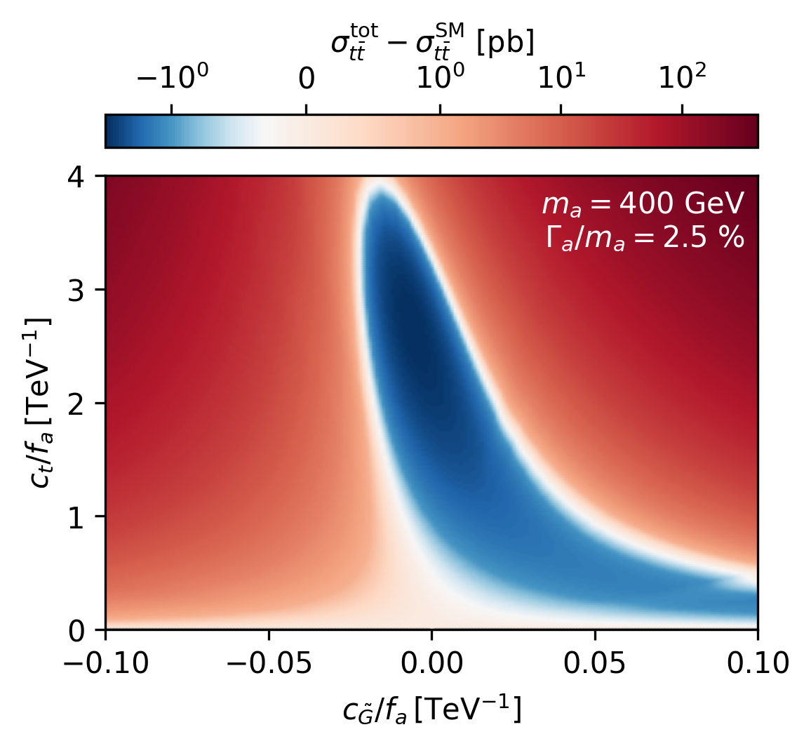
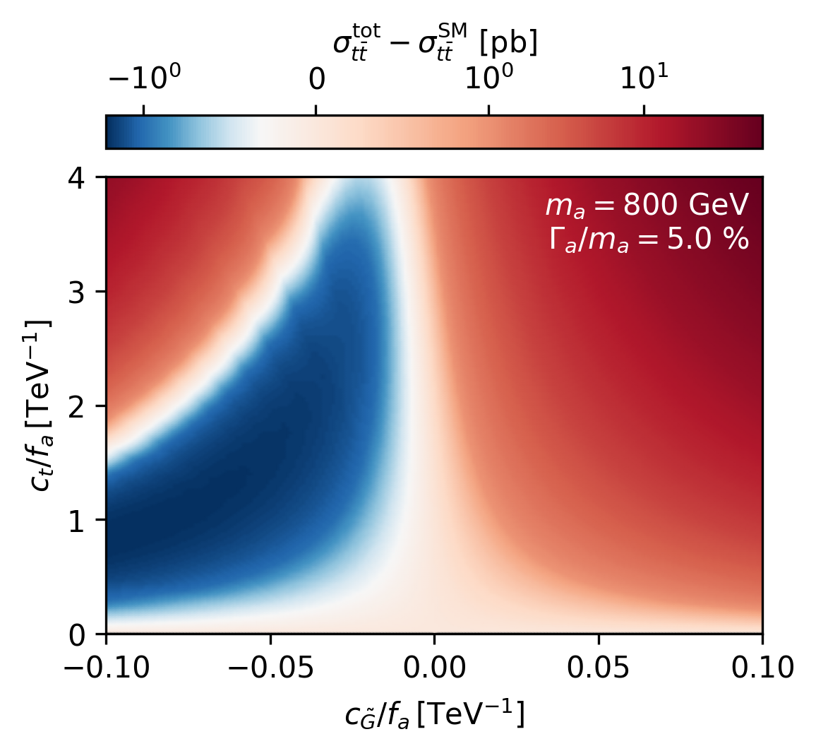
Figure 2: The background-subtracted inclusive $pp\to{t\bar{t}}$ cross section, including resonant $pp\to a$ production and ALP/SM interference, $\sigma_{t\bar{t}}^{\rm tot}-\sigma_{t\bar{t}}^{\rm SM}$, is shown in the plane of the ALP couplings $c_{{\tilde{G}}}/f_{a}$ and $c_{t}/f_{a}$ for different ALP masses and relative widths of $400\ \mathrm{GeV}$ and 2.5% (left) as well as $800\ \mathrm{GeV}$ and 5.0% (right). Negative values of $c_{t}$ are not shown as the cross section is symmetric under the sign change of both $c_{t}$ and $c_{{\tilde{G}}}$, see Eq. (14).

The results for the inclusive ${t\bar{t}}$ cross section incorporating the contributions from the resonant ALP signal and the ALP/SM interference, while the cross section corresponding to the SM ${t\bar{t}}$ background is subtracted, can be seen in Fig. 2 for the two ALP masses and widths of $m_{a}=400\ \mathrm{GeV}$, $\Gamma_{a}/m_{a}=2.5$% (left) and $m_{a}=800\ \mathrm{GeV}$, $\Gamma_{a}/m_{a}=5.0$% (right). The background-subtracted result $\sigma_{t\bar{t}}^{\rm tot}-\sigma_{t\bar{t}}^{\rm SM}$ is seen to be negative in a part of the $(c_{\tilde{G}}/f_{a},c_{t}/f_{a})$ parameter plane. This is due to the destructive interference between the diagrams shown in Fig. 1 and the SM diagrams contributing to $t\bar{t}$ production.

Explicitly, the background-subtracted inclusive cross section for the $400\ \mathrm{GeV}$, 2.5% case can be parameterized as

$$\sigma_{t\bar{t}}^{\rm tot}-\sigma_{t\bar{t}}^{\rm SM}= \Bigg{\{}\left[0.109c_{t}^{4}+22.3c_{t}^{3}c_{{\tilde{G}}}+1960c_{t}^{2}c_{{\tilde{G}}}^{2}\right]\left(\frac{\text{TeV}}{f_{a}}\right)^{4}$$

$$-\left[1.20c_{t}^{2}+97.2c_{t}c_{{\tilde{G}}}\right]\left(\frac{\text{TeV}}{f_{a}}\right)^{2}\Bigg{\}}\text{ pb}\,.$$ (14)

Note the symmetry of the the cross section under the sign change of both $c_{t}$ and $c_{{\tilde{G}}}$.

Following the CMS search for a heavy pseudoscalar Higgs boson [74], we discriminate the signal and background events based on two variables, the invariant mass of the ${t\bar{t}}$ system, $m_{{t\bar{t}}}$, and the spin correlation variable $c_{\mathrm{hel}}$. The latter is defined as

$$c_{\mathrm{hel}}=\cos{\varphi}=\hat{\ell}^{+}\cdot\hat{\ell}^{-}~{},$$ (15)

where $\varphi$ denotes the angle between the directions of flight $\hat{\ell}^{+}$ and $\hat{\ell}^{-}$ of the two leptons, defined respectively in the rest frames of their parent top or anti-top quarks. It can be shown that the distribution of this variable (without phase space cuts) has the form [120]

$$\frac{1}{\sigma}\frac{d\sigma}{dc_{\mathrm{hel}}}=\frac{1}{2}\left(1-D\,c_{\mathrm{hel}}\right)\ ,$$ (16)

where the slope $D$ is sensitive to the parity of a possible intermediate particle (in this case, the ALP or a pseudoscalar Higgs boson). Thus, this observable can be used to discriminate between the signal and the SM background.

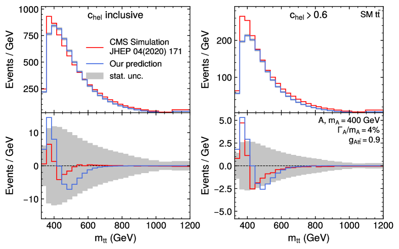
Figure 3: Differential distribution in $m_{{t\bar{t}}}$ for the SM (top) and for a pseudoscalar Higgs boson with $m_{A}=400\ \mathrm{GeV}$, 4.0% width and a coupling strength of $g_{{A{t\bar{t}}}}=0.9$, where the SM background has been subtracted (bottom). The left plot shows the distribution inclusive in the variable $c_{\mathrm{hel}}$, while the right plot shows it after selecting only events with $c_{\mathrm{hel}}>0.6$. Our smeared prediction (blue) is compared to the CMS simulation taken from [74] (red). All predictions are shown for an integrated luminosity of $35.9\,\mathrm{fb}^{-1}$. The gray bands show the expected statistical uncertainty from the SM ${t\bar{t}}$ background.

In order to account for the finite detector resolution we apply a Gaussian smearing with a standard deviation of $\sigma=15\%$ on $m_{{t\bar{t}}}$ . The magnitude of the smearing was extracted from a fit of the smeared generator predictions to both the SM ${t\bar{t}}$ background and the pseudoscalar Higgs-boson signal after the full detector simulation in Ref. [74]. A comparison between our $m_{{t\bar{t}}}$ distribution prediction and the CMS simulation is shown in Fig. 3. Note that we perform this comparison for $\Gamma_{a}/m_{a}=4\%$ as distributions for lower values of the relative width are not displayed in Ref. [74]. In the left panel, we show the distribution inclusive in $c_{\mathrm{hel}}$. In the right panel, we show the distribution after the cut $c_{\mathrm{hel}}>0.6$, highlighting the discrimination power of this variable. We will employ this cut for the rest of our analysis. While some discrepancy for the signal can be seen for the case of the (less sensitive) $c_{\mathrm{hel}}$-inclusive prediction, the distributions agree rather well with each other for $c_{\mathrm{hel}}>0.6$. For the SM background, some differences are present just above the ${t\bar{t}}$ threshold, which are expected to result from the details of the ${t\bar{t}}$ reconstruction in the experimental analysis.

We further approximate the experimental acceptance and efficiency for both signal and ${t\bar{t}}$ background as 10.6% before the $c_{\mathrm{hel}}$ requirement based on the numbers reported by CMS [74]. This acceptance is defined as the fraction of ${t\bar{t}}\rightarrow b\bar{b}\ell^{+}\ell^{-}\nu\bar{\nu}$ events ($\ell$ being electrons, muons or leptonically decaying taus) that pass all triggers and analysis cuts and contribute to the likelihood fit.

2.5 Systematic uncertainties

In analyzing the discrimination between a BSM signal and the SM expectation, we consider the following sources of systematic uncertainties:

• Unknown higher-order corrections in the calculation of both the signal and the ${t\bar{t}}$ background. In both cases, the corresponding uncertainties are estimated by varying the renormalization and factorization scales independently up and down by a factor of 2.

• The uncertainty in the PDF choice is estimated as the envelope of 100 pseudo-Hessian NNPDF 3.1 replicas, as recommended in Ref. [121].

• The value of the top-quark mass assumed in the simulation of the SM ${t\bar{t}}$ background. It is set to $m_{t}=172.5$ GeV by default and assigned a Gaussian uncertainty of $1\ \mathrm{GeV}$, as in Ref. [74].

• The uncertainty of the total rate of the SM ${t\bar{t}}$ background. It is taken as a log-normal uncertainty of 6% as in Ref. [74]. The inclusion of this uncertainty does not significantly influence our results.

Among these, the top-quark mass uncertainty is of particular importance for ALPs or pseudoscalar Higgs bosons with masses close to the ${t\bar{t}}$ production threshold, where the $m_{{t\bar{t}}}$ distribution for the SM ${t\bar{t}}$ background is strongly affected by even small variations in the top-quark mass for low $m_{{t\bar{t}}}$ values. In Fig. 4 on the left, we show the effect of such a variation for a luminosity of 35.9 $\mathrm{fb}^{-1}$, and compare it to the effect of a pseudoscalar Higgs-boson signal corresponding to the excess observed by CMS in the first-year Run 2 analysis [74]. As expected, we find that the top-quark mass variation has significant effects on the bins close to the ${t\bar{t}}$ threshold. The comparison with the expected signal for a pseudoscalar Higgs boson at 400 GeV shows that the variation of the top-quark mass in the SM background by $-1\ \mathrm{GeV}$ yields, after subtracting the SM background with $m_{t}=172.5\ \mathrm{GeV}$, some similarity with the peak–dip structure that is expected for the signal.

Since the effects of experimental cuts are taken into account only using acceptance factors, variations in acceptance due to the top-quark mass dependence are not included in our analysis. In particular, lowering the top-quark mass will result in lower transverse momenta of the top-quark decay products (leptons and jets), which in an experimental analysis would result in more events being rejected by triggers and lepton or jet quality cuts. This in return would mitigate the steep increase of observed events for low $m_{{t\bar{t}}}$ shown as the blue line in Fig. 4 (left). Similarly, the opposite is true for raising the top-quark mass (green line), in total leading to a smaller uncertainty due to the top quark mass. In addition to this, our method imposes the requirement $c_{\mathrm{hel}}>0.6$, while the experimental analysis considers the full range in $c_{\mathrm{hel}}$, split into five bins. A pseudoscalar Higgs boson signal is expected to contribute mostly for high $c_{\mathrm{hel}}$, while a variation due to a shift in the top mass affects all $c_{\mathrm{hel}}$ bins similarly, which gives additional power to distinguish the signal from a variation in the top-quark mass. As a result of both these effects, the uncertainty due to the top-quark mass is likely overestimated in our setup, and we will consider our results both including and excluding the uncertainty stemming from the top-quark mass in the following.

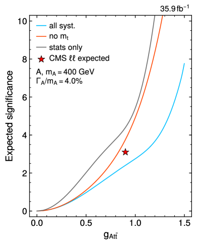
Figure 4: Left: The effect of a top-quark mass variation of $\pm 1\ \mathrm{GeV}$ in the SM ${t\bar{t}}$ background (green and blue lines; the central value is indicated by the black line in the upper plot, all displayed SM curves are normalized such that they yield the same total cross section) compared to the effect of a pseudoscalar Higgs boson with $m_{A}=400\ \mathrm{GeV}$, 4% width and $g_{{A{t\bar{t}}}}=0.9$ (red dashed line). The gray band in the lower plot, where the SM background has been subtracted, indicates the statistical uncertainty for an integrated luminosity of $35.9\,\mathrm{fb}^{-1}$. Right: The expected significance for the pseudoscalar Higgs boson as a function of its coupling $g_{{A{t\bar{t}}}}$ for the full set of systematic uncertainties, the full set except for the top-quark mass uncertainty, and for the case where only statistical uncertainties are taken into account. The expected significance reported by CMS for $g_{{A{t\bar{t}}}}=0.9$ is shown as the red star.

In order to compute expected significances and limits including the systematic uncertainties, we perform hypothesis tests based on a binned profile likelihood fit with the package pyhf [122, 123]. The expected number of events (SM background, resonant ALP production, and ALP–SM interference) in each bin of the differential distribution in $m_{{t\bar{t}}}$, as shown in Fig. 3, can be parameterized as a polynomial in the two ALP couplings $c_{t}/f_{a}$ and $c_{{\tilde{G}}}/f_{a}$. With this, we define the likelihood

$$\mathcal{L}(c_{t},c_{{\tilde{G}}},\theta_{j})=\prod_{i}\mathrm{Poisson}(N^{\mathrm{obs}}_{i}|N^{\mathrm{pred}}_{i}(c_{t},c_{{\tilde{G}}},\theta_{j}))\times\prod_{j}p(\theta_{j})\ ,$$ (17)

where $N^{\mathrm{obs}}_{i}$ is the observed number of events in bin $i$, $N^{\mathrm{pred}}_{i}$ is the predicted number of events for given values of the couplings, and $\theta_{j}$ are nuisance parameters encoding different theory-based systematic uncertainties as discussed above along with their corresponding prior distributions $p(\theta_{j})$. These are given by log-normal (for the ${t\bar{t}}$ rate uncertainty) or Gaussian (for all other uncertainties) distributions, with standard deviations as given above. Both shape and rate effects of the different uncertainty sources $\theta_{j}$ are fully taken into account in the predicted number of events $N^{\mathrm{pred}}_{i}(c_{t},c_{{\tilde{G}}},\theta_{j})$. For the HL-LHC projection all systematic uncertainties are halved since the accuracy of the theoretical predictions is expected to improve significantly on the relevant timescales. In the fit, the likelihood $\mathcal{L}$ is optimized simultaneously as a function of the couplings $c_{t}/f_{a},\,c_{{\tilde{G}}}/f_{a}$ and the nuisance parameters $\theta_{j}$.

In order to derive an expected limit for the ALP couplings, we define a test statistic $t_{c_{t},c_{{\tilde{G}}}}$ [124] as the profile likelihood ratio

$$t_{c_{t},c_{{\tilde{G}}}}=\min_{\theta_{j}}\left(-2\ln\frac{\mathcal{L}(c_{t},c_{{\tilde{G}}},\theta_{j})}{\hat{\mathcal{L}}}\right)\ ,$$ (18)

where

$$\hat{\mathcal{L}}=\max_{\hat{c}_{t},\hat{c}_{\tilde{G}},\hat{\theta}_{j}}\mathcal{L}(\hat{c}_{t},\hat{c}_{\tilde{G}},\hat{\theta}_{j})$$ (19)

is the value of the likelihood at the best-fit coupling and nuisance parameter values for given observed data. With this setup, the test statistic $t_{c_{t},c_{{\tilde{G}}}}$ is a measure of the agreement between the observed data and the ALP prediction for given couplings $c_{t}$ and $c_{{\tilde{G}}}$, taking into account systematic uncertainties.

To compute the expected significance for the detection of an ALP signal for given values of the ALP couplings, we assume that the observed data is equal to the prediction of the sum of the ALP signal and the SM ${t\bar{t}}$ background, and perform a hypothesis test for the background-only hypothesis, i.e. for the test statistic $t_{0,0}$ as defined in Eq. (18). The significance for rejecting the background-only hypothesis is given by $\sqrt{t_{0,0}}$ in this case.

We show the expected significance at a luminosity of $35.9\,\mathrm{fb}^{-1}$ for a pseudoscalar Higgs boson with $m_{A}=400\ \mathrm{GeV}$, $4.0\%$ width and varying coupling modifiers $g_{{A{t\bar{t}}}}$ (related to $c_{t}/f_{a}$ via Eq. (6)) in Fig. 4 on the right for different uncertainty models: with all systematic uncertainties including the one stemming from the top-quark mass, excluding the one from the top-quark mass, and with statistical uncertainties only. For $g_{{A{t\bar{t}}}}=0.9$, corresponding to the CMS excess, we find an expected significance of 2.3 standard deviations if all uncertainties including the one from the top-quark mass are taken into account, and 3.7 standard deviations for the case where the systematic uncertainty arising from the top-quark mass is not included. Comparing this to the expected significance in the di-lepton channel reported by CMS of 3.1 standard deviations [74], we find that the value that was obtained in the experimental analysis lies between our estimates when including or excluding the top-quark mass uncertainty. This is in line with our expectation, as mentioned above, that we overestimate the effect of top-quark mass variations because we do not incorporate acceptance effects. For the projected limits and significances that we will present below we will always quote the significances both including and excluding this uncertainty.

We also compute the significances for distinguishing a general ALP $a$ from a pseudoscalar Higgs boson $A$ with couplings $c_{t}/f_{a}=g_{{A{t\bar{t}}}}/v$ and $c_{{\tilde{G}}}=0$ (see Eq. (6)). Similarly to the definitions above (Eq. (18)), we assume the observed data to be equal to the expectation for the ALP, and calculate the expected significance for rejecting the pseudoscalar Higgs boson hypothesis as $\sqrt{t_{c_{t},c_{{\tilde{G}}}=0}}$.

3 Results

In this section we present the resulting limits on the Wilson coefficients of the ALP Lagrangian given in Eq. (4) and analyze the sensitivity for distinguishing between an ALP with non-vanishing $c_{{\tilde{G}}}$ coupling and a pseudoscalar Higgs boson of an extended Higgs sector for which $c_{{\tilde{G}}}=0$.

3.1 Translation of pseudoscalar Higgs boson limits

Since the additional pseudoscalar Higgs boson considered in Ref. [74] and an ALP exhibit the same coupling structure for $c_{\tilde{G}}=0$, the existing limits on the process $pp\rightarrow A\rightarrow t\bar{t}$ can be directly translated in this case into the first experimentally observed upper limits on the ALP coupling to the top quark using Eq. (6). In Fig. 5 we show the expected (black dashed) and observed (blue) upper limits on $c_{t}/f_{a}$ as a function of the ALP mass $m_{a}$ assuming a total relative width of $\Gamma_{a}/m_{a}=2.5$% and $\Gamma_{a}/m_{a}=5$% in the left and the right plot, respectively, based on the results of the CMS search for additional Higgs bosons in $t\bar{t}$ final states using $35.9~{}\mathrm{fb}^{-1}$ of data [74]. Also shown are the $1\sigma$ and $2\sigma$ uncertainty bands of the expected limits as green and yellow bands, respectively. Coupling values for which the predicted total width of the ALP, taking into account the $a\to{t\bar{t}}$, $a\to gg$ and $a\to\gamma\gamma$ decays, is larger than the assumed total width are indicated by the gray hatched band.

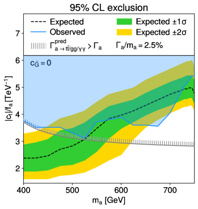
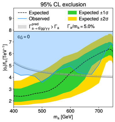
Figure 5: Limit on the coupling of an ALP to the top quark, $c_{t}/f_{a}$, in the case $c_{{\tilde{G}}}=0$, translated from Ref. [74], for a relative ALP width of 2.5% (left) and 5% (right). The hatched band shows the region in which the sum of the predicted partial widths for the $a\to{t\bar{t}},gg,\gamma\gamma$ decays exceeds the assumed total width.

In the left plot of Fig. 5 we can observe that in the ALP mass region $400\ \mathrm{GeV}<m_{a}\lesssim 550\ \mathrm{GeV}$ upper limits of $|c_{t}|/f_{a}$ between 3.0 and 3.8 $\ \mathrm{TeV}^{-1}$ are found. The expected limit in this mass region of $|c_{t}|/f_{a}\lesssim 2.5\ \mathrm{TeV}^{-1}$ is substantially smaller than the observed limits. This is a manifestation of the local excess observed by CMS (which, however, is not supported by the preliminary ATLAS result [75]). For larger masses the expected and observed limits are located in the parameter region where the predicted total width is larger than the assumed total width, so that no limits on $|c_{t}|/f_{a}$ that are compatible with the assumption of a 2.5% total width can be inferred. In the right plot a relative ALP width of 5% is assumed. In the mass range $400\ \mathrm{GeV}<m_{a}\lesssim 550\ \mathrm{GeV}$, where both the expected and the observed limit lie below the hatched band (and therefore the obtained results are compatible with the assumption of a 5% total width) coupling values of $|c_{t}|/f_{a}\gtrsim 4\ \mathrm{TeV}^{-1}$ are excluded.

3.2 Discrimination between an ALP and a 2HDM pseudoscalar Higgs boson

We now consider the case of an additional effective ALP–gluon coupling, $c_{{\tilde{G}}}\neq 0$, and investigate the sensitivity for distinguishing an ALP from a pseudoscalar Higgs boson with the same mass and total width and for which we assume $c_{{\tilde{G}}}=0$. Using the MC simulation described in Sect. 2.4, we analyze the resulting differences in the $m_{{t\bar{t}}}$ distribution.

We show in Fig. 6 the $m_{{t\bar{t}}}$ distributions after the cut $c_{\mathrm{hel}}>0.6$ for a pseudoscalar Higgs boson $A$ and for an ALP $a$ both with a mass of $400\ \mathrm{GeV}$, for several benchmark values of $c_{{\tilde{G}}}/f_{a}$ and $c_{t}/f_{a}$, given in Tab. 1. In each plot panel, the coupling $g_{A{t\bar{t}}}$ of the pseudoscalar Higgs boson is chosen such that its total cross-section contribution matches the one of the ALP for each benchmark. Two separate vertical axes show the background-subtracted number of events for two different choices of the integrated luminosity: $138~{}\mathrm{fb}^{-1}$ (Run 2) and $3~{}\mathrm{ab}^{-1}$ (HL-LHC). The light and dark shaded gray areas show the statistical uncertainty on the SM background corresponding to the two luminosity assumptions.

$a$		$A$
$c_{t}/f_{a}\,[\text{TeV}^{-1}]$	$c_{{\tilde{G}}}/f_{a}\,[\text{TeV}^{-1}]$	$g_{A{t\bar{t}}}$	$(\sigma^{\text{tot}}-\sigma^{\text{SM}})$ [pb]
$3.0$	$+0.015$	$0.95$	$+6.7$
$3.0$	$-0.015$	$0.43$	$-2.7$
$1.0$	$+0.025$	$0.75$	$-1.7$
$1.0$	$-0.025$	$0.87$	$+2.0$

Table 1: BSM cross-section contributions in the four considered parameter benchmarks for the ALP and pseudoscalar Higgs boson. The coupling $g_{{A{t\bar{t}}}}$ of the pseudoscalar Higgs boson is chosen such that its total cross-section contribution matches the one of the ALP for each benchmark.

For the pseudoscalar Higgs boson $A$ (dashed) a characteristic peak–dip structure located around the particle mass occurs in the $m_{{t\bar{t}}}$ distribution for sufficiently large values of $g_{{A{t\bar{t}}}}$ (upper left and lower right plot). For small values of $g_{{A{t\bar{t}}}}\lesssim 0.8$ (upper right and lower left plot), the depth of the dip, induced by the interference term, dominates over the height of the peak, which is mostly caused by contributions from the resonance term, leading to a deficit of events throughout most of the considered $m_{{t\bar{t}}}$ distribution.

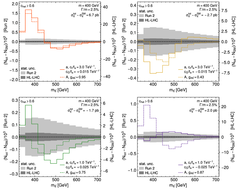
Figure 6: Differential distribution in $m_{{t\bar{t}}}$ for an ALP with different values of $c_{{\tilde{G}}}$ and $c_{t}$ and a pseudoscalar Higgs boson with different values of $g_{{A{t\bar{t}}}}$, both with a mass of $400\ \mathrm{GeV}$ and a total width of 2.5%. The couplings $c_{{\tilde{G}}}$, $c_{t}$ and $g_{{A{t\bar{t}}}}$ are chosen in the considered benchmark scenarios such that the ALP and the pseudoscalar Higgs boson have the same integrated cross section in a given panel. Event counts are shown for integrated luminosities corresponding to Run 2 ($138\,\mathrm{fb}^{-1}$, left axis) and the HL-LHC ($3\,\mathrm{ab}^{-1}$, right axis). The gray bands indicate the expected statistical uncertainties on the SM background for the two integrated luminosities.

Comparing the distributions of an ALP where $c_{{\tilde{G}}}\neq 0$ with those of a pseudoscalar Higgs boson, differences in the $m_{{t\bar{t}}}$ distributions become visible. In particular, if $c_{{\tilde{G}}}$ and $c_{t}$ have opposite sign, instead of the peak–dip structure a dip–peak structure may occur (upper right and lower right plots in Fig. 6). As expected, the differences between the distributions for an ALP and a pseudoscalar Higgs boson become more pronounced with increasing $|c_{{\tilde{G}}}|$ (lower left and lower right plots). For the upper left and upper right plots, the $a$ and $A$ distributions are qualitatively similar, featuring a peak–dip and dip–dominated structure, respectively. However, the position and depth of the dip as well as the high-mass tail of the distribution are different for the case where $c_{t}$ and $c_{{\tilde{G}}}$ have opposite signs (upper right plot). In the lower left plot, the ALP features a peak–dip structure, while the corresponding distribution for a pseudoscalar Higgs boson is dominated by a dip only. The most prominent difference in the distributions for an ALP and a pseudoscalar Higgs boson can be observed in the lower right plot. In this case, the $m_{{t\bar{t}}}$ distribution of the pseudoscalar Higgs boson features a peak–dip structure, while for the ALP a dip–peak structure occurs. In comparison to the indicated statistical uncertainties on the SM background for the two luminosity assumptions one can see that there is a certain sensitivity for discriminating between the hypothetical observation of an ALP and of a pseudoscalar Higgs boson already with the projection of the CMS analysis to the full Run 2 luminosity, and good prospects for all displayed scenarios for the case of the HL-LHC. These findings will be further quantified in the following.

In Tab. 2, we present the expected significances for the observation of an ALP or a pseudoscalar Higgs boson for three different integrated luminosities corresponding to Run 2, Run 2+3 and the HL-LHC. Analogously to Section 2.5, we present the significances for three different assumptions on the uncertainties: i) including statistical and all systematic uncertainties, ii) including statistical and systematic uncertainties but excluding the top-quark mass uncertainty, iii) considering statistical uncertainties only. In addition, as discussed in Sect. 2.5, we scale all systematic uncertainties by a factor of 0.5 for our projection to the HL-LHC in order to account for future improvements in prediction and analysis techniques. We find that the benchmark scenario with $c_{t}/f_{a}=3\ \mathrm{TeV}^{-1},c_{{\tilde{G}}}/f_{a}=0.015\ \mathrm{TeV}^{-1}$ can be distinguished from the SM expectation with a significance much above $5\,\sigma$ at the HL-LHC for the case where all systematic and statistical uncertainties are taken into account. For all the other displayed benchmark scenarios an expected sensitivity at the HL-LHC above the level of $5\,\sigma$ can be achieved if the uncertainty arising from the top-quark mass in the analysis can be significantly reduced compared to our simple estimate (see the discussion above). As indicated in the “no $m_{t}$ column”, for some of the displayed benchmark scenarios this level of significance could be reached in this case already with the integrated luminosity from Run 2 and Run 3.

Turning to the question of how well an ALP and a pseudoscalar Higgs boson can be distinguished from one another in the considered benchmark scenarios, the comparison of the predicted distributions for an ALP and a pseudoscalar Higgs boson in Fig. 6 with the statistical uncertainty (gray bands) shows that for the data that has been recorded at Run 2 the deviation between an ALP and a pseudoscalar Higgs boson is largest in comparison to the statistical uncertainty for the benchmark scenario with $c_{{\tilde{G}}}/f_{a}=-0.015\ \mathrm{TeV}^{-1}$, $c_{t}/f_{a}=3.0\ \mathrm{TeV}^{-1}$ (lower right plot of Fig. 6). In this case the peak–dip structure caused by the pseudoscalar Higgs boson would be expected to be well separable from the background, while the ALP produced with the same total cross section would give rise to a dip–peak structure that is significantly less pronounced. At the HL-LHC, all considered ALP benchmarks will be distinguishable from their pseudoscalar Higgs boson counterparts. More quantitatively, the significances for this comparison are given in Tab. 3. After LHC Runs 2(+3), only the benchmark scenario with $c_{t}/f_{a}=1\ \mathrm{TeV}^{-1}$ and $c_{{\tilde{G}}}/f_{a}=-0.025\ \mathrm{TeV}^{-1}$ has the potential to be distinguished from the case of a pseudoscalar Higgs boson with the same total cross section with (close to) $5\,\sigma$ significance. For all four considered benchmark scenarios, a $5\,\sigma$ distinction of an ALP from a pseudoscalar Higgs boson with $c_{{\tilde{G}}}=0$ will be possible at the HL-LHC, based on the result taking into account all systematic and statistical uncertainties. We note that in this case, as discussed above, the ALP signal itself may not be detectable with $5\,\sigma$ significance.

In case a new particle is detected at the LHC, the sensitivity for distinguishing between an ALP and a pseudoscalar Higgs boson would have an important impact on the future collider programme at the high-energy frontier. If one can show that only an ALP with $c_{{\tilde{G}}}\neq 0$ is in agreement with the experimental data, this could imply the existence of additional heavy BSM particles that are responsible for the additional contributions to the ALP–gluon contact interaction in the ALP EFT. The size of $c_{{\tilde{G}}}/f_{a}$ which is consistent with the data could then be used to gain information on whether these BSM particles could potentially be in reach of the LHC or other future colliders that are currently discussed.

$a$		$A$		Significance ($a$/$A$ vs. SM)
$c_{t}/f_{a}\,[\text{TeV}^{-1}]$	$c_{{\tilde{G}}}/f_{a}\,[\text{TeV}^{-1}]$	$g_{{A{t\bar{t}}}}$	Luminosity	all syst.	no $m_{t}$	stats only
$3.0$	$+0.015$	$0.95$	Run 2	$3.9$/$3.3$	$>10$/$8.9$	$>10$/$>10$
			Run 2+3	$5.2$/$4.3$	$>10$/$>10$	$>10$/$>10$
			HL-LHC	$>10$/$>10$	$>10$/$>10$	$>10$/$>10$
$3.0$	$-0.015$	$0.43$	Run 2	$2.1$/$1.2$	$2.2$/$1.5$	$4.4$/$2.9$
			Run 2+3	$3.0$/$1.5$	$3.0$/$2.0$	$6.5$/$4.3$
			HL-LHC	$8.7$/$4.2$	$8.8$/$5.7$	$>10$/$>10$
$1.0$	$+0.025$	$0.75$	Run 2	$1.1$/$2.4$	$2.6$/$4.7$	$4.0$/$6.3$
			Run 2+3	$1.4$/$3.1$	$3.2$/$6.0$	$5.9$/$9.4$
			HL-LHC	$3.9$/$8.4$	$8.2$/$>10$	$>10$/$>10$
$1.0$	$-0.025$	$0.87$	Run 2	$0.7$/$2.8$	$1.7$/$6.9$	$2.8$/$9.8$
			Run 2+3	$0.9$/$3.6$	$2.2$/$8.6$	$4.1$/$>10$
			HL-LHC	$2.3$/$9.9$	$5.5$/$>10$	$>10$/$>10$

Table 2: Significances for detecting an ALP or a pseudoscalar Higgs boson with a mass of 400 GeV and a width of 2.5% for the benchmark scenarios considered in Fig. 6. Three different treatments of the uncertainties as defined in Sect. 2.5 are shown. For the HL-LHC projection, all systematic uncertainties are scaled by a factor of 0.5. The “/” separates the significances of the ALP from those of the pseudoscalar Higgs boson.

$a$		$A$		Significance ($a$ vs. $A$)
$c_{t}/f_{a}\,[\text{TeV}^{-1}]$	$c_{{\tilde{G}}}/f_{a}\,[\text{TeV}^{-1}]$	$g_{{A{t\bar{t}}}}$	Luminosity	all syst.	no $m_{t}$	stats only
$3.0$	$+0.015$	$0.95$	Run 2	$1.3$	$1.9$	$3.3$
			Run 2+3	$1.8$	$2.3$	$4.9$
			HL-LHC	$5.3$	$5.7$	$>10$
$3.0$	$-0.015$	$0.43$	Run 2	$1.2$	$1.9$	$3.3$
			Run 2+3	$1.7$	$2.4$	$4.9$
			HL-LHC	$5.0$	$6.0$	$>10$
$1.0$	$+0.025$	$0.75$	Run 2	$1.5$	$2.3$	$2.7$
			Run 2+3	$2.0$	$3.1$	$3.9$
			HL-LHC	$5.8$	$8.8$	$>10$
$1.0$	$-0.025$	$0.87$	Run 2	$3.7$	$9.0$	$>10$
			Run 2+3	$4.6$	$>10$	$>10$
			HL-LHC	$>10$	$>10$	$>10$

Table 3: Significances for the discrimination of an ALP and a pseudoscalar Higgs boson for the benchmark scenarios considered in Fig. 6. The uncertainties are treated as in Tab. 2.

3.3 Projected ALP limits

As seen in Fig. 6, the LHC results of Run 2 and Run 3 and especially of the future high-luminosity phase are expected to yield significant improvements of the sensitivity to the ALP couplings $c_{{\tilde{G}}}$ and $c_{t}$. To quantify this, we derive estimates for the projected limits on the ALP couplings from the investigated $a\to{t\bar{t}}$ searches.

To this end, we use the same uncertainty setup as presented in Sect. 2.5 for computing significances. In a first step, we do not incorporate the systematic uncertainty arising from the top-quark mass. We assume that the observed data is equal to the SM expectation, i.e. that no deviation from the SM is found, and scan over values of the ALP couplings $c_{{\tilde{G}}}/f_{a}$ and $c_{t}/f_{a}$, each time performing a $\mathrm{CL_{s}}$ test [125, 126] using the test statistic given in Eq. (18). We assume the test statistic to be $\chi^{2}$-distributed with two degrees of freedom, and reject a set of values for the ALP couplings at 95% confidence level (CL) if the $\mathrm{CL_{s}}$ value for these couplings falls below a threshold of 0.05.

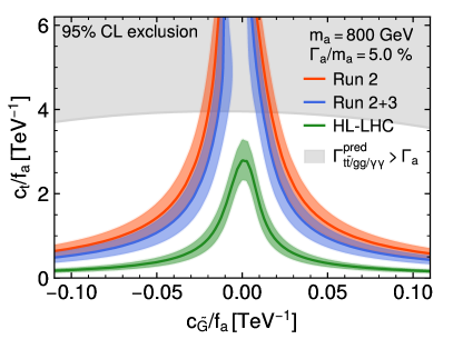
Figure 7: Projected expected limits on the ALP couplings $c_{{\tilde{G}}}/f_{a}$ and $c_{t}/f_{a}$ as obtained by the maximum likelihood fit for three different integrated luminosities, corresponding to LHC Run 2 (red), Run 2+3 (blue) and HL-LHC (green), and for $m_{a}=400\ \mathrm{GeV}$, $\Gamma_{a}/m_{a}=2.5\%$ (left) and $800\ \mathrm{GeV}$, $\Gamma_{a}/m_{a}=5.0\%$ (right). The shaded bands show the variations of the expected limit by one standard deviation. For all cases, all systematic uncertainties are included (scaled by a factor of 0.5 for the HL-LHC) except for the top-quark mass uncertainty. The region in which the assumed ALP width is lower than the total predicted width, taking into account the $a\to{t\bar{t}}$, $a\to gg$ and $a\to\gamma\gamma$ decays, is shown as the gray shaded area. In the left plot, the benchmark points from Fig. 6, with the same color coding, are shown as stars.

The projected limits resulting from this procedure are shown in Fig. 7 for $m_{a}=400\ \mathrm{GeV}$, $\Gamma_{a}/m_{a}=2.5\%$ (left plot) and $m_{a}=800\ \mathrm{GeV}$, $\Gamma_{a}/m_{a}=5\%$ (right plot). In both cases, we include all systematic uncertainties except for the top-quark mass uncertainty, as discussed in Sect. 2.5. For Run 2, we find a limit of $c_{t}/f_{a}\leq 3.5\ \mathrm{TeV}^{-1}$ for $m_{a}=400\ \mathrm{GeV}$ in the least sensitive case for $c_{{\tilde{G}}}$ (corresponding to values of $c_{{\tilde{G}}}/f_{a}=-0.02\ \mathrm{TeV}^{-1}$), while the limit is improved to $c_{t}/f_{a}\leq 0.34\ \mathrm{TeV}^{-1}$ for $|c_{{\tilde{G}}}|/f_{a}=0.1\ \mathrm{TeV}^{-1}$. For $m_{a}=800\ \mathrm{GeV}$, we find a limit of $c_{t}/f_{a}\leq 0.7\ \mathrm{TeV}^{-1}$ for $|c_{{\tilde{G}}}|/f_{a}=0.1\ \mathrm{TeV}^{-1}$, while no limit for the assumed total width can be set for $c_{{\tilde{G}}}=0$. The fact that the lowest sensitivity on $c_{t}$ is reached for a non-zero value of $c_{{\tilde{G}}}$ for $m_{a}=400\ \mathrm{GeV}$ results from a destructive signal–signal interference between the two possible production diagrams, which suppresses the signal cross section for small negative values of $c_{{\tilde{G}}}$. The four points indicated by stars in the left plot correspond to the four benchmark scenarios considered in Fig. 6. The red benchmark point and possibly also the green one can be probed already with the data from Run 2. The yellow benchmark point should become accessible with the integrated luminosity after Run 3 of the LHC, while the purple one becomes only accessible at the HL-LHC.

It should be noted that for $m_{a}=800\ \mathrm{GeV}$ and $\Gamma_{a}/m_{a}=5\%$, similar to Fig. 5, the expected exclusion limits on $c_{t}/f_{a}$ for Run 2 and Run 3 within the interval $|c_{{\tilde{G}}}|/f_{a}\leq 0.02$ lie in the region where the predicted total ALP decay width exceeds the width assumed in the analysis. For the integrated luminosities expected at the HL-LHC limits for both ALP masses can be set throughout the whole parameter space without a conflict with the assumed value for the total width. For the HL-LHC we find a significantly improved limit of $c_{t}/f_{a}\leq 1.4\,(2.8)\ \mathrm{TeV}^{-1}$ for $m_{a}=400\,(800)\ \mathrm{GeV}$. For $|c_{{\tilde{G}}}|/f_{a}=0.1\ \mathrm{TeV}^{-1}$, we find a limit of $c_{t}/f_{a}\leq 0.11\,(0.19)\ \mathrm{TeV}^{-1}$.

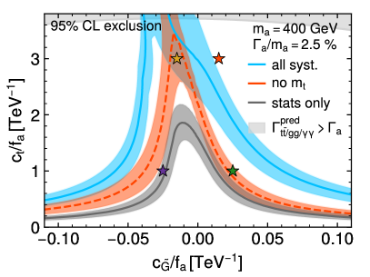
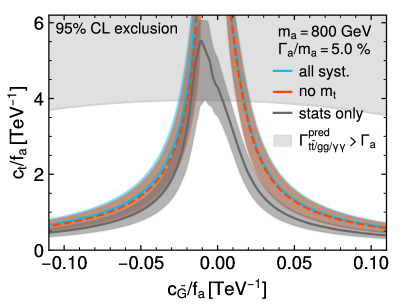
Figure 8: Projected expected limits on the ALP couplings $c_{{\tilde{G}}}/f_{a}$ and $c_{t}/f_{a}$ that are obtained as in Fig. 7, for $m_{a}=400\ \mathrm{GeV}$, $\Gamma_{a}/m_{a}=2.5\%$ (left plot) and $m_{a}=800\ \mathrm{GeV}$, $\Gamma_{a}/m_{a}=5\%$ (right plot) and for three different treatments of the uncertainties as defined in Sect. 2.5: with all systematic uncertainties including the top-quark mass uncertainty (blue), excluding the top-quark mass uncertainty but keeping other uncertainties (red), and considering statistical uncertainties only (gray). All limits are shown for an integrated luminosity of $138\,\mathrm{fb}^{-1}$, corresponding to Run 2.

We now analyze the impact of the treatment of the uncertainties, in particular the effect of taking into account the systematic uncertainty arising from the top-quark mass. To this end, in Fig. 8 we show the same limits for an integrated luminosity corresponding to Run 2 for the three different treatments of the uncertainties as in Tabs. 2–3. For $m_{a}=400\ \mathrm{GeV}$ (left plot), i.e. close to the ${t\bar{t}}$ production threshold, it can be seen that including the top-quark mass uncertainty significantly weakens the projected limits. As discussed in Sect. 2.5, this uncertainty is likely overestimated in our analysis, and we expect the limits that would be found in an experimental analysis to lie between the cases including or excluding the top-quark mass uncertainty (blue and red lines).

For $m_{a}=800\ \mathrm{GeV}$ (right plot), on the other hand, it can be seen that the effect of the top-quark mass uncertainty is very small. For this mass, the signal does not manifest itself as a peak–dip structure close to the ${t\bar{t}}$ production threshold and thus has a very different shape compared to modifications of the $m_{t\bar{t}}$ distribution caused by a variation of the mass of the top quark.

3.4 Comparison with other experimental limits

In this section we compare the projected limits on the ALP couplings obtained in the previous section to other current experimental limits on these parameters. Focusing on an ALP at $m_{a}=400\ \mathrm{GeV}$ and a relative width of $\Gamma_{a}/m_{a}=2.5\%$, we show in Fig. 9 our projected 95% CL limits on the coupling coefficients $c_{{\tilde{G}}}/f_{a}$ and $c_{t}/f_{a}$ based on the $pp\to a\to t\bar{t}$ process for an integrated luminosity of $138~{}\mathrm{fb}^{-1}$ collected during Run 2 (as shown by the red curve in Fig. 7). For the specific scenario of the top-philic ALP (see Eq. (7)), indicated by the black dot-dashed line, we find from the intersection with the red curve a projected limit of $c_{t}/f_{a}<1.7\ \mathrm{TeV}^{-1}$, which is complementary to the limit set at lower masses in Ref. [56]. Our limits are compared with the current limits resulting from LHC searches for di-photon resonances [88] (green shaded area) and from the measurement of the total cross section for the production of four top quarks [89] (blue shaded area), both based also on $138~{}\mathrm{fb}^{-1}$. Moreover, we depict the indirect limit on $c_{t}/f_{a}$, which is approximately independent of $c_{{\tilde{G}}}/f_{a}$ for $m_{a}=400\ \mathrm{GeV}$, resulting from a global analysis of ALP–SMEFT interference effects [44] (hatched gray line). In the following we briefly summarize how the existing exclusion regions displayed in Fig. 9 were obtained and discuss the assumptions on which they are based.

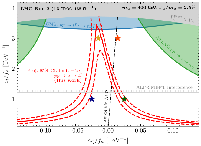
Figure 9: Limits on the ALP Wilson coefficients $c_{t}/f_{a}$ and $c_{{\tilde{G}}}/f_{a}$ from various sources: The red line shows our result for the projected expected 95% CL upper limit on the ALP couplings $c_{{\tilde{G}}}/f_{a}$ and $c_{t}/f_{a}$ from ALP searches in the invariant $t\bar{t}$ mass distribution and angular correlations for an ALP with a mass of $400\ \mathrm{GeV}$ and relative width of $2.5\%$ for the case where all statistical and systematic uncertainties are included except for the top-quark mass uncertainty (see Fig. 7). The red dashed lines indicate the $\pm 1\sigma$ uncertainty band. The green shaded areas are excluded at 95% CL from LHC searches for narrow di-photon resonances performed by ATLAS [88], and the blue shaded area is excluded from the CMS cross section measurement for the production of four top quarks [89], where both analyses are based on the full Run 2 dataset. Values of $c_{t}/f_{a}$ above the gray hatched line are excluded by ALP–SMEFT interference effects [44] (see text for details). Coupling values for which the predicted sum of the partial widths for $a\to{t\bar{t}},gg,\gamma\gamma$ is larger than the assumed total width of the ALP are indicated with the gray shaded area. The black dot-dashed line represents the couplings corresponding to a top-philic ALP.

Direct searches for resonant $gg\to a\to\gamma\gamma$ production

As explained above, the ALP coupling to top quarks induces at the one-loop level a coupling of the ALP to two photons, see Eq. (10). Searches for the ALP as a narrow di-photon resonance profit from a relatively small background, while interference effects between ALP production and the SM background are negligible. Existing LHC searches for high-mass di-photon resonances can therefore be used as a different way for probing ALPs as considered here. However, the di-photon branching ratio is strongly suppressed for ALP masses above the ${t\bar{t}}$ threshold. For an ALP mass of $m_{a}=400\ \mathrm{GeV}$ we can apply the 95% CL cross-section limits resulting from the ATLAS high-mass di-photon resonance search [88] as implemented in HiggsTools [127, 128, 129, 130, 131, 132]. We obtain the theoretical prediction for the resonant cross section of the ALP in the same way as described in Sect. 2.4, i.e. we compute the resonant gluon-fusion production cross-section at LO with MadGraph 5 and apply a $K$-factor $K_{\mathrm{res}}$ to account for higher-order QCD effects. As described in Sect. 2.3, the prediction for the decay $a\to\gamma\gamma$ is based on the loop-induced coupling involving the top-quark loop.

We stress again in this context that we treat the total width of the ALP as a free parameter in our analysis. Accordingly, for the coupling regions below the gray area in Fig. 9, where the predicted sum of the partial widths for the $t\bar{t}$, $gg$ and $\gamma\gamma$ decays is smaller than the assumed total width, the ALP would necessarily feature additional couplings to other SM or BSM particles. If those additional couplings of the ALP involve charged particles, the partial width for $a\to\gamma\gamma$ would receive additional loop-induced contributions besides the contribution from the top-quark loop. As a consequence, the exclusion regions resulting from the di-photon searches shown in Fig. 9 can be significantly modified via the impact of additional ALP couplings on the di-photon branching ratio.

Direct sensitivity to $a\to t\bar{t}$ in the production of four top quarks

At $m_{a}=400\ \mathrm{GeV}$ and assuming $\Gamma_{a}/m_{a}=2.5\%$, the ALP investigated here mainly decays into top-quark pairs. For the case where the ALP is produced in association with two top quarks, this decay mode contributes to the production of four top quarks at the LHC. This final state was recently measured for the first time using the Run 2 dataset collected at 13 TeV by both the CMS [89, 134] and the ATLAS [135, 136] collaborations. These measurements can be used to set upper limits on the process $pp\to t\bar{t}a\to t\bar{t}t\bar{t}$. The exclusion region shown in Fig. 9 is based on the CMS measurement in the same-sign di-lepton plus multilepton channel [89], which has the smallest statistical and systematic uncertainties among the currently existing measurements. CMS found a cross section of $\sigma_{t\bar{t}t\bar{t}}=17.7^{+4.4}_{-4.0}~{}\mathrm{fb}$, which agrees with the SM prediction $\sigma_{t\bar{t}t\bar{t}}^{\rm SM}=13.4~{}\mathrm{fb}$ [137] at about the level of $1\,\sigma$. We use as an upper limit on the cross section the upper value of the $2\,\sigma$ uncertainty band, which corresponds approximately to a 95% CL limit. As a simple estimate of the theoretical prediction for the ALP model, the cross section for $pp\to t\bar{t}a\to t\bar{t}t\bar{t}$ is added to the cross section that is predicted within the SM. This is conservative in the sense that taking into account a lower acceptance for events arising from the resonant process of ALP production than for the non-resonant SM-like contribution is expected to reduce the impact of this constraint on the displayed parameter space. Since for the final state with four top quarks the interference effects between the resonant ALP contribution and the non-resonant SM background are much less important compared to the case of $t\bar{t}$ production, they have been neglected here. The cross section for the production of the ALP in association with two top quarks was obtained with the help of HiggsTools as a function of $c_{t}$, and the decay width for $a\to t\bar{t}$ was computed according to Eq. (11) as in our analysis for the ${t\bar{t}}$ final state. The resulting exclusion limit only mildly depends on $c_{{\tilde{G}}}$ since $c_{{\tilde{G}}}$ enters this process only in the branching ratio for the $a\to{t\bar{t}}$ decay, which is the dominant decay mode for the considered coupling values. We find that the exclusion limit from the measurement of the production of four top quarks is significantly weaker than our projected limit from the $t\bar{t}$ searches except for the region of small negative values of $c_{{\tilde{G}}}/f_{a}$ where the latter limit is weakest. The limit on $c_{t}/f_{a}$ that we obtain for $c_{{\tilde{G}}}=0$ can be furthermore compared to limits that CMS has obtained in a search for new spin-0 particles in final states with three or four top quarks published in Ref. [138]. CMS found in the 2HDM interpretation a lower limit of $\tan\beta=1.2$ at a mass of 400 GeV (see upper right plot of Fig. 8 therein), which in terms of the ALP Wilson coefficients corresponds to a limit of $c_{t}/f_{a}=3.4$. This is in good agreement with the limit that we have obtained using the total cross section measurement of Ref. [89].

Indirect effects from ALP–SMEFT interference

ALP couplings can also be constrained indirectly through their impact on observables described in the SMEFT framework. The RG evolution induces non-zero SMEFT coefficients at scales probed at LEP or the LHC even if the ALP couplings are the only BSM contributions present at the UV scale [43]. This effect has been used to constrain the Wilson coefficients of the ALP effective Lagrangian by reinterpreting SMEFT constraints from LHC Higgs and top data as well as electroweak precision observables. The resulting bounds on ALP couplings to gluons and top quarks are [44]

$$|c_{t}|/f_{a}<1.2/\text{TeV},\,\qquad|c_{\tilde{G}}|/f_{a}<0.74/\text{TeV}\,,\quad {\rm for}\;m_{a}=400\,\text{GeV}$$

$$|c_{t}|/f_{a}<1.3/\text{TeV},\,\qquad|c_{\tilde{G}}|/f_{a}<0.83/\text{TeV}\,,\quad {\rm for}\;m_{a}=800\,\text{GeV}\,.$$ (20)

The limit on $c_{t}$ is dominated by its contribution to the SMEFT Wilson coefficient $C_{HD}$ corresponding to the SMEFT operator

$$\mathcal{O}_{HD}=(H^{\dagger}D_{\mu}H)^{*}(H^{\dagger}D^{\mu}H)\,,$$ (21)

which is tightly constrained from electroweak precision observables, most notably from the $W$-boson mass. For $c_{{\tilde{G}}}$ the reinterpretation of Higgs limits on $C_{uG}$, $C_{HG}$, corresponding to the dimension-six SMEFT operators

$$\mathcal{O}_{HG}=\left(\phi^{\dagger}\phi\right)\,G^{a}_{\mu\nu}G^{a\mu\nu}\,,\quad\mathcal{O}_{uG}=\left(\bar{Q}_{L}\sigma_{\mu\nu}u_{R}\right)T^{a}\tilde{\phi}\,G^{a\mu\nu}\,,$$ (22)

dominates the bounds. While these bounds are independent of, for instance, the ALP decay width or its branching ratios, they assume that all SMEFT Wilson coefficients are exactly zero at the high scale $\Lambda=4\pi f_{a}$. However, the presence of additional non-zero SMEFT Wilson coefficients at $\Lambda$ can influence the limits on the ALP coefficients $c_{t}$ and $c_{\tilde{G}}$ in either direction.

One can see in Fig. 9 that the expected limits from an investigation of the invariant $t\bar{t}$ mass distribution (red line) are substantially stronger than current limits both from LHC searches for narrow resonances decaying into two photons (green shaded area), and from the cross section measurement for the production of four top quarks (blue shaded area). Only in the region where the limits from the $m_{t\bar{t}}$ distribution become weak, i.e. for small values of $c_{{\tilde{G}}}$, the limits from the searches for four top quarks become comparable. The projected limits obtained in our analysis are the only limits from direct searches at the LHC that are comparable or stronger than the indirect limits on $c_{t}/f_{a}$ from the ALP–SMEFT interference effects (gray hatched line). We find limits on $c_{t}/f_{a}$ that are up to an order of magnitude stronger than the indirect bound on $c_{t}/f_{a}$ for values of $|c_{{\tilde{G}}}|/f_{a}\gtrsim 0.05$, whereas for smaller values of $|c_{{\tilde{G}}}|/f_{a}$ the indirect limit from the ALP–SMEFT interference is stronger.

4 Summary and Conclusion

Axion-like particles (ALPs) are singlets under the SM gauge groups and appear in many well-motivated extensions of the SM as the lightest degree of freedom due to their nature as pseudo-Nambu-Goldstone bosons of an approximate axion shift-symmetry. Therefore, ALPs are an attractive target for the LHC and the HL-LHC in the hunt for BSM physics. In this paper we studied the gluon-fusion production of an ALP at the LHC with subsequent decay into a pair of top quarks. This channel is directly sensitive to both the ALP–fermion and the ALP–gluon couplings in the production, and to the ALP–fermion coupling in the decay. Motivated by recent searches for additional Higgs bosons in $t\bar{t}$ final states by the ATLAS and CMS collaborations, we have analyzed the current limits and future prospects for probing the parameter space of the effective ALP Lagrangian.

We have performed a recasting of the published CMS search for a CP-odd Higgs boson, extending it to the case of an ALP with a more general coupling structure. In our simulation the decay of the top quarks has been included, thus going beyond previous phenomenological studies of ALP searches in $m_{t\bar{t}}$ distributions. Since top quarks decay on timescales much smaller than the one of the strong interaction, angular variables of the decay products can be used to gain sensitivity to spin information of the top quarks. This information can be utilized to enhance the sensitivity for discriminating a signal from the background and for characterizing the properties of a possible signal. Exploiting the information from the invariant-mass distribution of the final-state top quarks, $m_{t\bar{t}}$, and the spin correlation variable, $c_{\mathrm{hel}}$, we have investigated in particular how the production of an ALP with generic couplings to gluons and top quarks can be distinguished from the production of a pseudoscalar which couples to gluons exclusively via a top-quark loop.

In order to incorporate the effects of a finite detector resolution into our phenomenological analysis, we have applied a Gaussian smearing with $\sigma=15\%$ on the $m_{{t\bar{t}}}$ distribution. We determined the appropriate magnitude of the smearing from a fit of the smeared generator predictions to both the SM ${t\bar{t}}$ background and the expected signal for a CP-odd Higgs-boson that was obtained in the CMS analysis based on a full detector simulation. By comparing the distributions with and without imposing the cut $c_{\mathrm{hel}}>0.6$ on the helicity variable we have demonstrated the high discrimination power of this variable.

In our analysis we have investigated in detail different sources of systematic uncertainties. In this context we have pointed out in particular the importance of the systematic uncertainty that is associated with the uncertainty on the mass of the top quark, which strongly affects the $m_{{t\bar{t}}}$ distribution for the SM ${t\bar{t}}$ background in the low-mass region just above the ${t\bar{t}}$ threshold. In our phenomenological analysis we have used a Gaussian uncertainty of $\pm 1\ \mathrm{GeV}$ for the top-quark mass. For the example of an expected signal of a CP-odd Higgs boson at 400 GeV we have demonstrated that the variation of the top-quark mass in the SM background by $-1\ \mathrm{GeV}$ yields, after subtracting the SM background with $m_{t}=172.5\ \mathrm{GeV}$, a pattern resembling the peak–dip structure that is expected for the signal. Since in our phenomenological analysis, which does not take into account variations in the acceptance arising from the top-quark mass dependence, the uncertainty associated with the top-quark mass is likely to be overestimated, we have presented our results with and without the uncertainty stemming from the top-quark mass. In order to compute expected significances and limits including the systematic uncertainties, we have performed hypothesis tests based on a binned profile likelihood fit.

As a first step in our numerical analysis we have employed the results from the CMS search for a CP-odd Higgs boson using $35.9$ fb^-1 of data collected at $\sqrt{s}=13$ TeV (with a similar expected sensitivity as the preliminary Run 2 ATLAS result) to derive limits on the effective ALP Lagrangian in terms of the Wilson coefficient $c_{t}$ for the case $c_{{\tilde{G}}}=0$. For the example of an ALP in the mass range of $400\ \mathrm{GeV}<m_{a}\lesssim 550\ \mathrm{GeV}$ and with a relative width of 5%, coupling values of $|c_{t}|/f_{a}\gtrsim 4\ \mathrm{TeV}^{-1}$ are excluded. We have then investigated the expected significances for the observation of an ALP or a pseudoscalar Higgs boson for the integrated luminosities corresponding to Run 2 and Run 2$+$3 of the LHC as well as to the HL-LHC. For a benchmark scenario with $c_{t}/f_{a}=3\ \mathrm{TeV}^{-1}$ and $c_{{\tilde{G}}}/f_{a}=0.015\ \mathrm{TeV}^{-1}$, taking into account all systematic and statistical uncertainties, we have shown that the discrimination from the SM expectation is possible with very high significance at the HL-LHC. For all the other investigated benchmark scenarios for ALPs and pseudoscalar Higgs bosons we have found that an expected sensitivity at the HL-LHC above the level of $5\,\sigma$ can be achieved if the uncertainty arising from the top-quark mass in the analysis can be significantly reduced compared to our simple estimate. In this case such a level of significance could be reached already with the integrated luminosity from Run 2 and Run 3 for some of the investigated benchmark scenarios.

As a further step we determined the significances for distinguishing a generic ALP from a pseudoscalar Higgs boson that couples to gluons exclusively via a top-quark loop. We have found that at the HL-LHC all considered ALP benchmarks will be distinguishable from their pseudoscalar Higgs boson counterparts for the case where the latter have the same mass and relative width as the considered ALP and where the couplings are such that the integrated cross sections for the two types of BSM particles are the same. Already with the data from Run 2 and Run 3 of the LHC a significant sensitivity for distinguishing between an ALP and a pseudoscalar Higgs boson is achieved. We note that this kind of information can have important implications for the future collider programme at the high-energy frontier because of the different prospects for detecting additional BSM particles.

Turning from the prospects for discovering new particles to projected limits from ALP searches, we have determined projected limits on the ALP couplings to fermions and gluons in terms of the Wilson coefficients of the ALP–SM Lagrangian under the assumption that no deviations from the SM expectation will be observed. Including all systematic uncertainties except for the top-quark mass uncertainty, we have found for Run 2 a projected limit of $c_{t}/f_{a}\leq 3.5\ \mathrm{TeV}^{-1}$ for $m_{a}=400\ \mathrm{GeV}$ in the least sensitive case for $c_{{\tilde{G}}}$ (corresponding to values of $c_{{\tilde{G}}}/f_{a}=-0.02\ \mathrm{TeV}^{-1}$), while the limit is improved to $c_{t}/f_{a}\leq 0.34\ \mathrm{TeV}^{-1}$ for $|c_{{\tilde{G}}}|/f_{a}=0.1\ \mathrm{TeV}^{-1}$. For $m_{a}=800\ \mathrm{GeV}$ we have obtained a projected limit for Run 2 of $c_{t}/f_{a}\leq 0.7\ \mathrm{TeV}^{-1}$ for $|c_{{\tilde{G}}}|/f_{a}=0.1\ \mathrm{TeV}^{-1}$. For the HL-LHC we find a significantly improved projected limit of $c_{t}/f_{a}\leq 1.4\,(2.8)\ \mathrm{TeV}^{-1}$ for $m_{a}=400\,(800)\ \mathrm{GeV}$ and $c_{{\tilde{G}}}\approx 0$. For $|c_{{\tilde{G}}}|/f_{a}=0.1\ \mathrm{TeV}^{-1}$, we have obtained a projected limit of $c_{t}/f_{a}\leq 0.11\,(0.19)\ \mathrm{TeV}^{-1}$. Regarding the impact of taking into account the systematic uncertainty arising from the top-quark mass, as expected we have found significant effects for the case of $m_{a}=400\ \mathrm{GeV}$, i.e. close to the ${t\bar{t}}$ production threshold, while for $m_{a}=800\ \mathrm{GeV}$ this uncertainty has only a very small effect.

In order to assess the impact of our projected limits for Run 2 of the LHC, in a final step we have compared those limits from the $t\bar{t}$ searches (focusing on the case $m_{a}=400\ \mathrm{GeV}$) with existing experimental bounds from LHC searches for narrow di-photon resonances and from measurements of the production of four top quarks. We have also shown for comparison the constraints from global analyses of ALP–SMEFT interference effects, which arise from renormalization group running effects that induce a mixing between ALP EFT operators and SMEFT operators. We showed that our projected limits from the $t\bar{t}$ searches are significantly stronger than the ones from the measurement of the production of four top quarks except for the region of small negative values of $c_{{\tilde{G}}}/f_{a}$, where our projected limit from the $t\bar{t}$ searches is weakest. For the largest values of $|c_{{\tilde{G}}}|/f_{a}$ considered in our analysis, our projected limits from the $t\bar{t}$ searches are up to an order of magnitude stronger. The current limits from searches for $a\to\gamma\gamma$ (for the considered case that the di-photon decay of the ALP is only generated via the top-quark loop contribution) have turned out to be always substantially weaker compared to our projected limits from the $t\bar{t}$ searches. In comparison to the indirect limits obtained from ALP–SMEFT interference effects, which rely on the assumption that the ALP dimension five operators are the only BSM contribution present at the UV scale, we have found that the projected direct limits from the $t\bar{t}$ searches at the LHC are the only ones that can give rise to limits comparable or below the indirect limit on $c_{t}/f_{a}$ from ALP–SMEFT interference effects. Overall, the limits on $c_{t}/f_{a}$ that can be obtained from ALP searches in the $m_{t\bar{t}}$ distribution are expected to be the strongest limits in the range $c_{{\tilde{G}}}/f_{a}<-0.04\ \mathrm{TeV}^{-1}$ and $c_{{\tilde{G}}}/f_{a}>0.02\ \mathrm{TeV}^{-1}$.

To conclude, we derived limits on the ALP coupling to the top quark for ALPs with a mass above the ${t\bar{t}}$ threshold. First, we reinterpreted existing limits on pseudoscalar Higgs bosons for ALPs in the case where no contact interaction with gluons exists beyond the one induced by the top-quark loop. As the main part of our analysis, we explored the sensitivities to distinguish ALPs from heavy pseudoscalar Higgs bosons. Within the considered benchmark scenarios, we find that a distinction can be possible already using the LHC Run 2 dataset, with substantially improved prospects at the HL-LHC. Assuming the absence of a signal, we derived expected limits dependent on the ALP–top and ALP–gluon couplings which are significantly stronger than existing direct limits from other searches. They also complement indirect limits derived from ALP–SMEFT interference. We encourage the experimental collaborations to adopt the strategies outlined in our paper for future ALP searches at the LHC.

5 Acknowledgements

We thank Katharina Behr, Quentin Bonnefoy and Susanne Westhoff for useful discussions. A.B. is supported by the Cluster of Excellence “Precision Physics, Fundamental Interactions, and Structure of Matter” (PRISMA⁺ EXC 2118/1) funded by the German Research Foundation (DFG) within the German Excellence Strategy (Project ID 390831469). The work of T.B. is supported by the German Bundesministerium für Bildung und Forschung (BMBF, Federal Ministry of Education and Research) – project 05H21VKCCA. The work of S.H. has received financial support from the grant PID2019-110058GB-C21 funded by MCIN/AEI/10.13039/501100011033 and by “ERDF A way of making Europe”, and in part by by the grant IFT Centro de Excelencia Severo Ochoa CEX2020-001007-S funded by MCIN/AEI/10.13039/501100011033. S.H. also acknowledges support from Grant PID2022-142545NB-C21 funded by MCIN/AEI/10.13039/501100011033/ FEDER, UE. A.G., L.J., C.S. and G.W. acknowledge support by the Deutsche Forschungsgemeinschaft (DFG, German Research Foundation) under Germany‘s Excellence Strategy – EXC 2121 “Quantum Universe” – 390833306. This work has been partially funded by the Deutsche Forschungsgemeinschaft (DFG, German Research Foundation) - 491245950.

References

- [1] R.D. Peccei and H.R. Quinn, CP Conservation in the Presence of Instantons, Phys. Rev. Lett. 38 (1977) 1440.
- [2] R.D. Peccei and H.R. Quinn, Constraints Imposed by CP Conservation in the Presence of Instantons, Phys. Rev. D 16 (1977) 1791.
- [3] S. Weinberg, A New Light Boson?, Phys. Rev. Lett. 40 (1978) 223.
- [4] F. Wilczek, Problem of Strong and Invariance in the Presence of Instantons, Phys. Rev. Lett. 40 (1978) 279.
- [5] L. Di Luzio, M. Giannotti, E. Nardi and L. Visinelli, The landscape of QCD axion models, Phys. Rept. 870 (2020) 1 [2003.01100].
- [6] K. Choi, S.H. Im and C. Sub Shin, Recent Progress in the Physics of Axions and Axion-Like Particles, Ann. Rev. Nucl. Part. Sci. 71 (2021) 225 [2012.05029].
- [7] F. Chadha-Day, J. Ellis and D.J.E. Marsh, Axion dark matter: What is it and why now?, Sci. Adv. 8 (2022) abj3618 [2105.01406].
- [8] E. Witten, Some Properties of O(32) Superstrings, Phys. Lett. B 149 (1984) 351.
- [9] P. Svrcek and E. Witten, Axions In String Theory, JHEP 06 (2006) 051 [hep-th/0605206].
- [10] J.M. Frere, D.R.T. Jones and S. Raby, Fermion Masses and Induction of the Weak Scale by Supergravity, Nucl. Phys. B 222 (1983) 11.
- [11] J. Preskill, M.B. Wise and F. Wilczek, Cosmology of the Invisible Axion, Phys. Lett. B 120 (1983) 127.
- [12] L.F. Abbott and P. Sikivie, A Cosmological Bound on the Invisible Axion, Phys. Lett. B 120 (1983) 133.
- [13] M. Dine and W. Fischler, The Not So Harmless Axion, Phys. Lett. B 120 (1983) 137.
- [14] E. Katz, A.E. Nelson and D.G.E. Walker, The Intermediate Higgs, JHEP 08 (2005) 074 [hep-ph/0504252].
- [15] ATLAS collaboration, Search for Higgs boson decays into two new low-mass spin-0 particles in the 4 channel with the ATLAS detector using collisions at TeV, Phys. Rev. D 102 (2020) 112006 [2005.12236].
- [16] ATLAS collaboration, Search for Higgs boson decays into a pair of pseudoscalar particles in the final state with the ATLAS detector in collisions at =13 TeV, Phys. Rev. D 105 (2022) 012006 [2110.00313].
- [17] CMS collaboration, Search for an exotic decay of the Higgs boson to a pair of light pseudoscalars in the final state with two muons and two b quarks in pp collisions at 13 TeV, Phys. Lett. B 795 (2019) 398 [1812.06359].
- [18] ATLAS collaboration, Search for Higgs Boson Decays into a Boson and a Light Hadronically Decaying Resonance Using 13 TeV Collision Data from the ATLAS Detector, Phys. Rev. Lett. 125 (2020) 221802 [2004.01678].
- [19] ATLAS collaboration, Measurement of light-by-light scattering and search for axion-like particles with 2.2 nb-1 of Pb+Pb data with the ATLAS detector, JHEP 03 (2021) 243 [2008.05355].
- [20] CMS collaboration, Evidence for light-by-light scattering and searches for axion-like particles in ultraperipheral PbPb collisions at 5.02 TeV, Phys. Lett. B 797 (2019) 134826 [1810.04602].
- [21] V.A. Rubakov, Grand unification and heavy axion, JETP Lett. 65 (1997) 621 [hep-ph/9703409].
- [22] B. Holdom and M.E. Peskin, Raising the Axion Mass, Nucl. Phys. B 208 (1982) 397.
- [23] S. Dimopoulos, A. Hook, J. Huang and G. Marques-Tavares, A collider observable QCD axion, JHEP 11 (2016) 052 [1606.03097].
- [24] T. Gherghetta, N. Nagata and M. Shifman, A Visible QCD Axion from an Enlarged Color Group, Phys. Rev. D 93 (2016) 115010 [1604.01127].
- [25] H.M. Georgi, L.J. Hall and M.B. Wise, Grand Unified Models With an Automatic Peccei-Quinn Symmetry, Nucl. Phys. B 192 (1981) 409.
- [26] G. Lazarides, C. Panagiotakopoulos and Q. Shafi, Phenomenology and Cosmology With Superstrings, Phys. Rev. Lett. 56 (1986) 432.
- [27] R. Holman, S.D.H. Hsu, T.W. Kephart, E.W. Kolb, R. Watkins and L.M. Widrow, Solutions to the strong CP problem in a world with gravity, Phys. Lett. B 282 (1992) 132 [hep-ph/9203206].
- [28] S.M. Barr and D. Seckel, Planck scale corrections to axion models, Phys. Rev. D 46 (1992) 539.
- [29] S. Ghigna, M. Lusignoli and M. Roncadelli, Instability of the invisible axion, Phys. Lett. B 283 (1992) 278.
- [30] M. Kamionkowski and J. March-Russell, Planck scale physics and the Peccei-Quinn mechanism, Phys. Lett. B 282 (1992) 137 [hep-th/9202003].
- [31] A. Hook, S. Kumar, Z. Liu and R. Sundrum, High Quality QCD Axion and the LHC, Phys. Rev. Lett. 124 (2020) 221801 [1911.12364].
- [32] A. Valenti, L. Vecchi and L.-X. Xu, Grand Color axion, JHEP 10 (2022) 025 [2206.04077].
- [33] R.S. Bedi, T. Gherghetta and M. Pospelov, Enhanced EDMs from small instantons, Phys. Rev. D 106 (2022) 015030 [2205.07948].
- [34] Q. Bonnefoy, Heavy fields and the axion quality problem, Phys. Rev. D 108 (2023) 035023 [2212.00102].
- [35] K. Mimasu and V. Sanz, ALPs at Colliders, JHEP 06 (2015) 173 [1409.4792].
- [36] J. Jaeckel and M. Spannowsky, Probing MeV to 90 GeV axion-like particles with LEP and LHC, Phys. Lett. B 753 (2016) 482 [1509.00476].
- [37] I. Brivio, M.B. Gavela, L. Merlo, K. Mimasu, J.M. No, R. del Rey et al., ALPs Effective Field Theory and Collider Signatures, Eur. Phys. J. C 77 (2017) 572 [1701.05379].
- [38] M. Bauer, M. Neubert and A. Thamm, Collider Probes of Axion-Like Particles, JHEP 12 (2017) 044 [1708.00443].
- [39] N. Craig, A. Hook and S. Kasko, The Photophobic ALP, JHEP 09 (2018) 028 [1805.06538].
- [40] M. Bauer, M. Neubert, S. Renner, M. Schnubel and A. Thamm, Flavor probes of axion-like particles, JHEP 09 (2022) 056 [2110.10698].
- [41] M.B. Gavela, J.M. No, V. Sanz and J.F. de Trocóniz, Nonresonant Searches for Axionlike Particles at the LHC, Phys. Rev. Lett. 124 (2020) 051802 [1905.12953].
- [42] S. Carra, V. Goumarre, R. Gupta, S. Heim, B. Heinemann, J. Kuechler et al., Constraining off-shell production of axionlike particles with Z and WW differential cross-section measurements, Phys. Rev. D 104 (2021) 092005 [2106.10085].
- [43] A.M. Galda, M. Neubert and S. Renner, ALP — SMEFT interference, JHEP 06 (2021) 135 [2105.01078].
- [44] A. Biekötter, J. Fuentes-Martín, A.M. Galda and M. Neubert, A global analysis of axion-like particle interactions using SMEFT fits, JHEP 09 (2023) 120 [2307.10372].
- [45] T. Biswas, Probing the Interactions of Axion-Like Particles with Electroweak Bosons and the Higgs Boson in the High Energy Regime at LHC, 2312.05992.
- [46] K. Choi, S.H. Im, C.B. Park and S. Yun, Minimal Flavor Violation with Axion-like Particles, JHEP 11 (2017) 070 [1708.00021].
- [47] J. Martin Camalich, M. Pospelov, P.N.H. Vuong, R. Ziegler and J. Zupan, Quark Flavor Phenomenology of the QCD Axion, Phys. Rev. D 102 (2020) 015023 [2002.04623].
- [48] M. Chala, G. Guedes, M. Ramos and J. Santiago, Running in the ALPs, Eur. Phys. J. C 81 (2021) 181 [2012.09017].
- [49] M. Bauer, M. Neubert, S. Renner, M. Schnubel and A. Thamm, The Low-Energy Effective Theory of Axions and ALPs, JHEP 04 (2021) 063 [2012.12272].
- [50] C.D. Froggatt and H.B. Nielsen, Hierarchy of Quark Masses, Cabibbo Angles and CP Violation, Nucl. Phys. B 147 (1979) 277.
- [51] H. Georgi, D.B. Kaplan and L. Randall, Manifesting the Invisible Axion at Low-energies, Phys. Lett. B 169 (1986) 73.
- [52] T. Gherghetta and A. Pomarol, Bulk fields and supersymmetry in a slice of AdS, Nucl. Phys. B 586 (2000) 141 [hep-ph/0003129].
- [53] K. Agashe, R. Contino and A. Pomarol, The Minimal composite Higgs model, Nucl. Phys. B 719 (2005) 165 [hep-ph/0412089].
- [54] B. Gripaios, A. Pomarol, F. Riva and J. Serra, Beyond the Minimal Composite Higgs Model, JHEP 04 (2009) 070 [0902.1483].
- [55] F. Esser, M. Madigan, V. Sanz and M. Ubiali, On the coupling of axion-like particles to the top quark, JHEP 09 (2023) 063 [2303.17634].
- [56] S. Blasi, F. Maltoni, A. Mariotti, K. Mimasu, D. Pagani and S. Tentori, Top-philic ALP phenomenology at the LHC: the elusive mass-window, 2311.16048.
- [57] S. Bruggisser, L. Grabitz and S. Westhoff, Global analysis of the ALP effective theory, JHEP 01 (2024) 092 [2308.11703].
- [58] A.V. Phan and S. Westhoff, Precise tests of the axion coupling to tops, 2312.00872.
- [59] T. Ferber, A. Filimonova, R. Schäfer and S. Westhoff, Displaced or invisible? ALPs from B decays at Belle II, JHEP 04 (2023) 131 [2201.06580].
- [60] J.K. Behr and A. Grohsjean, Dark Matter Searches with Top Quarks, Universe 9 (2023) 16 [2302.05697].
- [61] L. Rygaard, J. Niedziela, R. Schäfer, S. Bruggisser, J. Alimena, S. Westhoff et al., Top Secrets: long-lived ALPs in top production, JHEP 10 (2023) 138 [2306.08686].
- [62] Y. Hosseini and M. Mohammadi Najafabadi, Prospects for Probing Axionlike Particles at a Future Hadron Collider through Top Quark Production, Universe 8 (2022) 301 [2208.00414].
- [63] S. Chigusa, S. Girmohanta, Y. Nakai and Y. Zhang, Aiming for tops of ALPs with a muon collider, JHEP 01 (2024) 077 [2310.11018].
- [64] C.-X. Yue, H. Wang and Y.-Q. Wang, Detecting the coupling of axion-like particles with fermions at the ILC, Phys. Lett. B 848 (2024) 138368 [2311.16768].
- [65] A. Biekötter, T. Biekötter, A. Grohsjean, S. Heinemeyer, L. Jeppe, C. Schwanenberger et al., Distinguishing Axion-Like Particles and 2HDM Higgs bosons in production at the LHC, PoS EPS-HEP2023 (2024) 474.
- [66] K.J.F. Gaemers and F. Hoogeveen, Higgs Production and Decay Into Heavy Flavors With the Gluon Fusion Mechanism, Phys. Lett. B 146 (1984) 347.
- [67] D. Dicus, A. Stange and S. Willenbrock, Higgs decay to top quarks at hadron colliders, Phys. Lett. B 333 (1994) 126 [hep-ph/9404359].
- [68] W. Bernreuther, M. Flesch and P. Haberl, Signatures of Higgs bosons in the top quark decay channel at hadron colliders, Phys. Rev. D 58 (1998) 114031 [hep-ph/9709284].
- [69] R. Frederix and F. Maltoni, Top pair invariant mass distribution: A Window on new physics, JHEP 01 (2009) 047 [0712.2355].
- [70] M. Carena and Z. Liu, Challenges and opportunities for heavy scalar searches in the channel at the LHC, JHEP 11 (2016) 159 [1608.07282].
- [71] A. Djouadi, J. Ellis, A. Popov and J. Quevillon, Interference effects in production at the LHC as a window on new physics, JHEP 03 (2019) 119 [1901.03417].
- [72] H. Bahl, R. Kumar and G. Weiglein, Analysis of interference effects in the di-top final state for CP-mixed scalars in extended Higgs sectors, PoS EPS-HEP2023 (2024) 057.
- [73] ATLAS collaboration, Search for Heavy Higgs Bosons Decaying to a Top Quark Pair in Collisions at with the ATLAS Detector, Phys. Rev. Lett. 119 (2017) 191803 [1707.06025].
- [74] CMS collaboration, Search for heavy Higgs bosons decaying to a top quark pair in proton-proton collisions at 13 TeV, JHEP 04 (2020) 171 [1908.01115].
- [75] ATLAS collaboration, Search for heavy neutral Higgs bosons decaying to a top quark pair in 140 fb-1 of proton-proton collision data at TeV, Tech. Rep. ATLAS-CONF-2024-001, CERN, Geneva (2024).
- [76] K. Behr, private communication.
- [77] T.D. Lee, A Theory of Spontaneous T Violation, Phys. Rev. D 8 (1973) 1226.
- [78] J.E. Kim, Weak Interaction Singlet and Strong CP Invariance, Phys. Rev. Lett. 43 (1979) 103.
- [79] G.C. Branco, P.M. Ferreira, L. Lavoura, M.N. Rebelo, M. Sher and J.P. Silva, Theory and phenomenology of two-Higgs-doublet models, Phys. Rept. 516 (2012) 1 [1106.0034].
- [80] D0 collaboration, Evidence for spin correlation in production, Phys. Rev. Lett. 108 (2012) 032004 [1110.4194].
- [81] CMS collaboration, Measurement of the top quark polarization and spin correlations using dilepton final states in proton-proton collisions at 13 TeV, Phys. Rev. D 100 (2019) 072002 [1907.03729].
- [82] ATLAS collaboration, Measurements of top-quark pair spin correlations in the channel at TeV using collisions in the ATLAS detector, Eur. Phys. J. C 80 (2020) 754 [1903.07570].
- [83] W. Bernreuther and A. Brandenburg, Tracing CP violation in the production of top quark pairs by multiple TeV proton proton collisions, Phys. Rev. D 49 (1994) 4481 [hep-ph/9312210].
- [84] V. Barger, T. Han and D.G.E. Walker, Top Quark Pairs at High Invariant Mass: A Model-Independent Discriminator of New Physics at the LHC, Phys. Rev. Lett. 100 (2008) 031801 [hep-ph/0612016].
- [85] E. Arganda, L. Da Rold, D.A. Díaz and A.D. Medina, Interpretation of LHC excesses in ditop and ditau channels as a 400-GeV pseudoscalar resonance, JHEP 11 (2021) 119 [2108.03058].
- [86] T. Biekötter, A. Grohsjean, S. Heinemeyer, C. Schwanenberger and G. Weiglein, Possible indications for new Higgs bosons in the reach of the LHC: N2HDM and NMSSM interpretations, Eur. Phys. J. C 82 (2022) 178 [2109.01128].
- [87] J.M. Connell, P. Ferreira and H.E. Haber, Accommodating hints of new heavy scalars in the framework of the flavor-aligned two-Higgs-doublet model, Phys. Rev. D 108 (2023) 055031 [2302.13697].
- [88] ATLAS collaboration, Search for resonances decaying into photon pairs in 139 fb-1 of collisions at =13 TeV with the ATLAS detector, Phys. Lett. B 822 (2021) 136651 [2102.13405].
- [89] CMS collaboration, Observation of four top quark production in proton-proton collisions at s=13TeV, Phys. Lett. B 847 (2023) 138290 [2305.13439].
- [90] Z. Berezhiani, L. Gianfagna and M. Giannotti, Strong CP problem and mirror world: The Weinberg-Wilczek axion revisited, Phys. Lett. B 500 (2001) 286 [hep-ph/0009290].
- [91] L. Gianfagna, M. Giannotti and F. Nesti, Mirror world, supersymmetric axion and gamma ray bursts, JHEP 10 (2004) 044 [hep-ph/0409185].
- [92] S.D.H. Hsu and F. Sannino, New solutions to the strong CP problem, Phys. Lett. B 605 (2005) 369 [hep-ph/0408319].
- [93] A. Hook, Anomalous solutions to the strong CP problem, Phys. Rev. Lett. 114 (2015) 141801 [1411.3325].
- [94] H. Fukuda, K. Harigaya, M. Ibe and T.T. Yanagida, Model of visible QCD axion, Phys. Rev. D 92 (2015) 015021 [1504.06084].
- [95] C.-W. Chiang, H. Fukuda, M. Ibe and T.T. Yanagida, 750 GeV diphoton resonance in a visible heavy QCD axion model, Phys. Rev. D 93 (2016) 095016 [1602.07909].
- [96] A. Kobakhidze, Heavy axion in asymptotically safe QCD, 1607.06552.
- [97] P. Agrawal and K. Howe, Factoring the Strong CP Problem, JHEP 12 (2018) 029 [1710.04213].
- [98] P. Agrawal and K. Howe, A Flavorful Factoring of the Strong CP Problem, JHEP 12 (2018) 035 [1712.05803].
- [99] M.K. Gaillard, M.B. Gavela, R. Houtz, P. Quilez and R. Del Rey, Color unified dynamical axion, Eur. Phys. J. C 78 (2018) 972 [1805.06465].
- [100] C. Csáki, M. Ruhdorfer and Y. Shirman, UV Sensitivity of the Axion Mass from Instantons in Partially Broken Gauge Groups, JHEP 04 (2020) 031 [1912.02197].
- [101] R.T. Co, L.J. Hall and K. Harigaya, Axion Kinetic Misalignment Mechanism, Phys. Rev. Lett. 124 (2020) 251802 [1910.14152].
- [102] T. Gherghetta and M.D. Nguyen, A Composite Higgs with a Heavy Composite Axion, JHEP 12 (2020) 094 [2007.10875].
- [103] A. Kivel, J. Laux and F. Yu, Supersizing axions with small size instantons, JHEP 11 (2022) 088 [2207.08740].
- [104] B. Gavela, P. Quílez and M. Ramos, The QCD axion sum rule, JHEP 04 (2024) 056 [2305.15465].
- [105] Q. Bonnefoy, C. Grojean and J. Kley, Shift-Invariant Orders of an Axionlike Particle, Phys. Rev. Lett. 130 (2023) 111803 [2206.04182].
- [106] M. Spira, A. Djouadi, D. Graudenz and P.M. Zerwas, Higgs boson production at the LHC, Nucl. Phys. B 453 (1995) 17 [hep-ph/9504378].
- [107] J. Alwall, R. Frederix, S. Frixione, V. Hirschi, F. Maltoni, O. Mattelaer et al., The automated computation of tree-level and next-to-leading order differential cross sections, and their matching to parton shower simulations, JHEP 07 (2014) 079 [1405.0301].
- [108] C. Degrande, C. Duhr, B. Fuks, D. Grellscheid, O. Mattelaer and T. Reiter, UFO - The Universal FeynRules Output, Comput. Phys. Commun. 183 (2012) 1201 [1108.2040].
- [109] J. Bonilla, I. Brivio, M.B. Gavela and V. Sanz, One-loop corrections to ALP couplings, JHEP 11 (2021) 168 [2107.11392].
- [110] P. Nason, A New method for combining NLO QCD with shower Monte Carlo algorithms, JHEP 11 (2004) 040 [hep-ph/0409146].
- [111] S. Frixione, P. Nason and C. Oleari, Matching NLO QCD computations with Parton Shower simulations: the POWHEG method, JHEP 11 (2007) 070 [0709.2092].
- [112] S. Alioli, P. Nason, C. Oleari and E. Re, A general framework for implementing NLO calculations in shower Monte Carlo programs: the POWHEG BOX, JHEP 06 (2010) 043 [1002.2581].
- [113] S. Frixione, P. Nason and G. Ridolfi, A Positive-weight next-to-leading-order Monte Carlo for heavy flavour hadroproduction, JHEP 09 (2007) 126 [0707.3088].
- [114] NNPDF collaboration, Parton distributions from high-precision collider data, Eur. Phys. J. C 77 (2017) 663 [1706.00428].
- [115] C. Bierlich et al., A comprehensive guide to the physics and usage of PYTHIA 8.3, 2203.11601.
- [116] D. Eriksson, J. Rathsman and O. Stal, 2HDMC: Two-Higgs-Doublet Model Calculator Physics and Manual, Comput. Phys. Commun. 181 (2010) 189 [0902.0851].
- [117] R.V. Harlander, S. Liebler and H. Mantler, SusHi: A program for the calculation of Higgs production in gluon fusion and bottom-quark annihilation in the Standard Model and the MSSM, Comput. Phys. Commun. 184 (2013) 1605 [1212.3249].
- [118] M. Czakon and A. Mitov, Top++: A Program for the Calculation of the Top-Pair Cross-Section at Hadron Colliders, Comput. Phys. Commun. 185 (2014) 2930 [1112.5675].
- [119] A. Banfi, N. Kauer, A. Lind, J.M. Lindert and R. Wood, Higgs interference effects in top-quark pair production in the 1HSM, 2309.16759.
- [120] W. Bernreuther, A. Brandenburg, Z.G. Si and P. Uwer, Top quark pair production and decay at hadron colliders, Nucl. Phys. B 690 (2004) 81 [hep-ph/0403035].
- [121] J. Butterworth et al., PDF4LHC recommendations for LHC Run II, J. Phys. G 43 (2016) 023001 [1510.03865].
- [122] L. Heinrich, M. Feickert and G. Stark, “pyhf: v0.7.4.” 10.5281/zenodo.1169739.
- [123] L. Heinrich, M. Feickert, G. Stark and K. Cranmer, pyhf: pure-Python implementation of HistFactory statistical models, Journal of Open Source Software 6 (2021) 2823.
- [124] G. Cowan, K. Cranmer, E. Gross and O. Vitells, Asymptotic formulae for likelihood-based tests of new physics, Eur. Phys. J. C 71 (2011) 1554 [1007.1727].
- [125] T. Junk, Confidence level computation for combining searches with small statistics, Nucl. Instrum. Meth. A 434 (1999) 435 [hep-ex/9902006].
- [126] A.L. Read, Presentation of search results: the CLs technique, Journal of Physics G: Nuclear and Particle Physics 28 (2002) 2693.
- [127] P. Bechtle, O. Brein, S. Heinemeyer, G. Weiglein and K.E. Williams, HiggsBounds: Confronting Arbitrary Higgs Sectors with Exclusion Bounds from LEP and the Tevatron, Comput. Phys. Commun. 181 (2010) 138 [0811.4169].
- [128] P. Bechtle, O. Brein, S. Heinemeyer, G. Weiglein and K.E. Williams, HiggsBounds 2.0.0: Confronting Neutral and Charged Higgs Sector Predictions with Exclusion Bounds from LEP and the Tevatron, Comput. Phys. Commun. 182 (2011) 2605 [1102.1898].
- [129] P. Bechtle, O. Brein, S. Heinemeyer, O. Stål, T. Stefaniak, G. Weiglein et al., : Improved Tests of Extended Higgs Sectors against Exclusion Bounds from LEP, the Tevatron and the LHC, Eur. Phys. J. C74 (2014) 2693 [1311.0055].
- [130] P. Bechtle, S. Heinemeyer, O. Stal, T. Stefaniak and G. Weiglein, Applying Exclusion Likelihoods from LHC Searches to Extended Higgs Sectors, Eur. Phys. J. C 75 (2015) 421 [1507.06706].
- [131] P. Bechtle, D. Dercks, S. Heinemeyer, T. Klingl, T. Stefaniak, G. Weiglein et al., HiggsBounds-5: Testing Higgs Sectors in the LHC 13 TeV Era, Eur. Phys. J. C 80 (2020) 1211 [2006.06007].
- [132] H. Bahl, T. Biekötter, S. Heinemeyer, C. Li, S. Paasch, G. Weiglein et al., HiggsTools: BSM scalar phenomenology with new versions of HiggsBounds and HiggsSignals, Comput. Phys. Commun. 291 (2023) 108803 [2210.09332].
- [133] CMS collaboration, Search for physics beyond the standard model in high-mass diphoton events from proton-proton collisions at 13 TeV, Phys. Rev. D 98 (2018) 092001 [1809.00327].
- [134] CMS collaboration, Evidence for four-top quark production in proton-proton collisions at s=13TeV, Phys. Lett. B 844 (2023) 138076 [2303.03864].
- [135] ATLAS collaboration, Measurement of the tt production cross section in collisions at = 13 TeV with the ATLAS detector, JHEP 11 (2021) 118 [2106.11683].
- [136] ATLAS collaboration, Observation of four-top-quark production in the multilepton final state with the ATLAS detector, Eur. Phys. J. C 83 (2023) 496 [2303.15061].
- [137] M. van Beekveld, A. Kulesza and L.M. Valero, Threshold Resummation for the Production of Four Top Quarks at the LHC, Phys. Rev. Lett. 131 (2023) 211901 [2212.03259].
- [138] CMS collaboration, Search for production of four top quarks in final states with same-sign or multiple leptons in proton-proton collisions at 13 TeV, Eur. Phys. J. C 80 (2020) 75 [1908.06463].
- [139] Particle Data Group collaboration, Review of Particle Physics, PTEP 2020 (2020) 083C01.
- [140] CDF collaboration, High-precision measurement of the boson mass with the CDF II detector, Science 376 (2022) 170.