Transitionless Quantum Driving of the Tomonaga-Luttinger Liquid

Abstract

Shortcuts to adiabaticity (STA) make the fast preparation of many-body states possible, circumventing the limitations of adiabatic strategies. We propose a fast STA protocol for generating interacting states in the Tomonaga-Luttinger liquid by counter-diabatic driving, stirring the dynamics with an auxiliary control field. To this end, we exploit the equivalence between the time-dependent Tomonaga-Luttinger liquid and an ensemble of quantum oscillators with driven mass and frequency. We specify the closed-form expression of the counterdiabatic control and demonstrate its efficiency in suppressing excitations.

Introduction.– Many-body quantum systems in low spatial dimensions are characterized by enhanced correlations in contrast to their three-dimensional counterparts. In one spatial dimension, the canonical Fermi liquid theory breaks down. In this setting, the Tomonaga-Luttinger liquid (TLL) provides a universal low-energy description of interacting fermions or bosons Tomonaga (1950); Luttinger (1963) in terms of bosonic collective degrees of freedom Mattis and Lieb (1965). Due to its broad applicability, the TLL has been used as a test-bed for nonequilibrium quantum phenomena in theoretical and experimental studies Giamarchi (2004); Iucci and Cazalilla (2009); Cazalilla et al. (2011); Guan et al. (2013); Cazalilla (2006); Cazalilla and Chung (2016); Kinoshita T (2006); Rigol et al. (2007); Kaminishi et al. (2015, 2018); Yamamoto et al. (2022). Works to date predominantly focus on the nonequilibrium dynamics of the TLL following a sudden interaction quench Dóra and Moessner (2017); Dóra (2014); Dóra et al. (2013); Bácsi and Dóra (2013); Dóra and Moca (2020); Bácsi et al. (2019); Pollmann et al. (2013); Kennes and Meden (2013); Nessi and Iucci (2013); Vu et al. (2020); Wei and Lu (2021), motivated by experimental progress Klanjšek et al. (2008); Rüegg et al. (2008). In addition, understanding the nonequilibrium dynamics induced by control protocols involving finite-time driving is often necessary for the preparation of many-body states, useful in quantum technologies ranging from quantum simulation to adiabatic quantum computing Albash and Lidar (2018); Carcy et al. (2021); Haller et al. (2010); Cedergren et al. (2017). Shortcuts to Adiabaticity (STA) offer an attractive framework for fast state preparation without the requirement for slow driving Chen et al. (2010); Torrontegui et al. (2013); del Campo and Kim (2019); Guéry-Odelin et al. (2019). A universal scheme for implementing STA relies on counter-diabatic driving (CD), which stirs the quantum evolution along the prescribed trajectory by using counterdiabatic controls Demirplak and Rice (2003, 2005, 2008); Berry (2009). While the application of STA by CD to many-body systems is generally challenging del Campo et al. (2012); Takahashi and del Campo (2024), it is largely facilitated in systems with continuous variables characterized by self-similar dynamics Chen et al. (2010); del Campo (2011); del Campo and Boshier (2012); Jarzynski (2013); del Campo (2013); Deffner et al. (2014). The latter naturally arises in certain systems of ultracold gases in time-dependent traps Kagan et al. (1996); Castin and Dum (1996); Deng et al. (2016). In these systems, STA schemes have been implemented with both weak and strong interactions Schaff et al. (2010, 2011a, 2011b); Rohringer et al. (2015); Deng et al. (2018a, b); Diao et al. (2018); Henson et al. (2018).

The distribution of energy scales in the TLL hampers the engineering of finite-time driving schemes as an alternative to adiabatic protocols. One approach relies on reverse engineering the TLL time evolution using a semiclassical sine-Gordon potential as an auxiliary control Dupays et al. (2024). As an alternative, CD provides a universal scheme for the engineering of STA. We focus on the engineering of STA in the TLL by counterdiabatic tailoring of the time-dependent interactions, paving the way to a manifold of applications ranging from optimal control Rahmani and Chamon (2011) to quantum thermodynamics Schmiedmayer (2018); Chen et al. (2019); Gluza et al. (2021). The TLL can describe the low-energy excitations of one-dimensional models such as the Lieb-Liniger Lieb (1963), the Tonks-Girardeau gas Tonks (1936); Girardeau (1960), the Fermi gas Bácsi et al. (2020), and the Bose-Hubbard model in the continuum Cazalilla (2003). CD in systems of continuous variables generally requires assisting the dynamics with velocity-dependent terms in the Hamiltonian description. In many important applications, such terms can be effectively realized by a local potential, making use of a rotating frame Torrontegui et al. (2013); del Campo (2013); Deffner et al. (2014). However, depending on the specific system, it may not be possible to recast the CD term in a local form, i.e., as an external potential or interaction term.

This work reports STA protocols for the CD preparation of many-body states in the interaction-driven TLL. After computing the counterdiabatic controls in closed form, we establish the link between this model and an ensemble of quantum oscillators with driven mass and frequencies. We demonstrate the influence of the CD protocol on the stability of the TLL and find a range of driving speeds for which the CD protocol is relevant. We then demonstrate its efficiency in suppressing nonadiabatic energy excitations and show that the form of the CD potential varies with the nature of the interactions.

Representations of the TLL Hamiltonian. Let us consider the driven TLL Hamiltonian, the derivation of which is reviewed in SM ; Iucci and Cazalilla (2009); Dupays et al. (2024),

$$H_{\rm TL}(t) =\sum_{p\neq 0}\hbar\omega(p,t)K_{0}(p)+\sum_{p\neq 0}\frac{\hbar g(p,t)}{2}\left[K_{-}(p)+K_{+}(p)\right]$$

$$-\sum_{p\neq 0}\frac{\hbar\omega(p,t)}{2},$$ (1)

where $v_{F}$ is the Fermi velocity. In terms of the interaction potentials $g_{2/4}(p,t)$, $\omega(p,t)=|p|\left[v_{F}+\frac{g_{4}(p,t)}{2\pi}\right]$ and $g(p,t)=|p|\frac{g_{2}(p,t)}{2\pi}$. The Hamiltonian (1) is spanned by the generators of the $\mathfrak{su}(1,1)$ group

$$K_{0}(p) =\frac{1}{2}\left[b^{\dagger}(p)b(p)+b^{\dagger}(-p)b(-p)+1\right],$$ (2)

$$K_{+}(p) =b^{\dagger}(p)b^{\dagger}(-p),\quad K_{-}(p)=b(p)b(-p),$$ (3)

that verify the commutation rules $[K_{0}(p),K_{\pm}(p)]=\pm K_{\pm}(p)$, $[K_{-}(p),K_{+}(p)]=2K_{0}(p)$. Alternatively, the TLL Hamiltonian can be written as a function of a phase operator $\phi(x)$ and its conjugated density fluctuation operator $\Pi(x)=\frac{\partial_{x}\theta(x)}{\pi}$, that verify the commutation relation $[\phi(x),\Pi(x^{\prime})]=i\delta(x-x^{\prime})$. Consider a momentum-independent interaction potential, satisfying $g_{2/4}(p,t)=\tilde{g}_{2/4}(t)$, where the tilde is used to clearly distinguish the coupling coefficients from the general $g_{2/4}(p,t)$. This corresponds to a contact interaction in real space for which the TLL Hamiltonian reads

$$H_{\rm TL}(t)=\frac{\hbar v_{s}(t)}{2}\int_{0}^{L}\left[\frac{\pi}{K(t)}\Pi(x)^{2}+\frac{K(t)}{\pi}(\partial_{x}\phi(x))^{2}\right]dx,$$

where the sound velocity $v_{s}$ and the Luttinger parameter $K$ are functions of the interaction potentials

CD control and the driven TLL. As a control approach, CD guides the nonadiabatic dynamics of a given system along a prescribed adiabatic trajectory Demirplak and Rice (2003, 2005, 2008); Berry (2009). It removes the requirement of slow driving in adiabatic methods by introducing auxiliary controls. Specifically, consider the adiabatic trajectory associated with a system described by the time-dependent Hamiltonian $H_{0}(t)=\sum_{n}E_{n}(t)|n(t)\rangle\langle n(t)|$. The adiabatic evolution associated to the Hamiltonian $H_{0}(t)$ is given by the state $|\Psi_{n}(t)\rangle=e^{i\theta_{n}(t)}e^{i\gamma_{n}(t)}|n(t)\rangle$ for an initial state in the $n$-th eigenstate $|n(0)\rangle$, with the dynamical phase $\theta_{n}(t)=-\frac{1}{\hbar}\int_{0}^{t}dt^{\prime}E_{n}(t^{\prime})$ and the Berry phase $\gamma_{n}(t)=i\int_{0}^{t}dt^{\prime}\langle n(t^{\prime})|\partial_{t^{\prime}}n(t^{\prime})\rangle$. The CD makes the adiabatic evolution to $H_{0}(t)$ the exact evolution when the dynamics is generated by the controlled Hamiltonian that reads $H(t)=H_{0}(t)+H_{\rm CD}(t)$, with the auxiliary CD term

$$H_{\rm CD}=i\hbar\sum_{n}\left(|\partial_{t}n\rangle\langle n|-\langle n|\partial_{t}n\rangle|n\rangle\langle n|\right),$$ (5)

where $|n\rangle=|n(t)\rangle$, for short. The instantaneous eigenstates of $H_{0}(t)$ can be written in terms of the evolution operator for parallel transport, $U_{t}=\sum_{n}|n(t)\rangle\langle n(0)|$ as $|n\rangle=U_{t}|n(0)\rangle$. As a result, the first CD term in Eq. (5) can be expressed as $i\hbar\sum_{n}|\partial_{t}n\rangle\langle n|=i\hbar\partial_{t}U_{t}U^{\dagger}_{t}$. Furthermore, the Berry phase can be written as the expectation value $-i\hbar\langle n(0)|U^{\dagger}_{t}\partial_{t}U_{t}|n(0)\rangle$.

Let us focus on the case of the driven TLL when $H_{0}(t)$ is given by $H_{\rm TL}(t)$ in Eq. (1). One can diagonalize the instantaneous TLL Hamiltonian (1) by applying the Bogoliubov transformation $U(\eta_{t})=\exp\left\{\sum_{p\neq 0}\frac{\eta_{t}}{2}[K_{+}(p)-K_{-}(p)]\right\}$ satisfying the condition $\tanh[2\eta_{t}]=-\frac{g(p,t)}{\omega(p,t)}$. We define the time-dependent bosonic operators $a(p,t)=U(\eta_{t})b(p)U^{\dagger}(\eta_{t})$, satisfying

$$a(p,t) =\cosh(\eta_{t})b(p)-\sinh(\eta_{t})b^{\dagger}(-p),$$ (6)

$$b(p) =\cosh(\eta_{t})a(p,t)+\sinh(\eta_{t})a^{\dagger}(-p,t).$$ (7)

After the Bogoliubov transformation, the Hamiltonian (1) can be brought to the diagonal form

$$H_{\rm TL}(t) = \sum_{p\neq 0}\epsilon(p,t)a^{\dagger}(p,t)a(p,t)+E_{0}(t),$$ (8)

with the ground state energy $E_{0}(t)=\frac{1}{2}\sum_{p\neq 0}\left[\epsilon(p,t)-\hbar\omega(p,t)\right]$, and $\epsilon(p,t)=\hbar\sqrt{[\omega(p,t)]^{2}-[g(p,t)]^{2}}$. In other words, the instantaneous evolution of the TLL can be seen as the Bogoliubov transformation of the free TLL Hamiltonian. As noticed in Haldane (1981), the ground state energy does not diverge if $\epsilon(p,t)$ tends to $\omega(p,t)$ for high momenta.

Counterdiabatic control using invariant of motions. The CD guides the nonadiabatic dynamics of the TLL along the prescribed adiabatic trajectory. The latter can be built from a unitary evolution. The supplementary gauge potential due to the nonadiabatic dynamics gives rise to the CD Hamiltonian. To formalize this idea, we exploit the theory of invariants of motions developed by Lewis and Riesenfeld for the $SU(1,1)$ dynamical group Lewis and Riesenfeld (1969a), as further described in SM . Making use of the initial invariant of motion $I^{0}=\sum_{p\neq 0}\hbar\omega_{0p}K_{0}(p)$, upon rescaling $I^{0}/\sigma^{2}_{t}$ with a scalar function $\sigma_{t}$, we build the dynamics for the interaction quench using a unitary time-evolution operator corresponding to a Bogoliubov transformation $Q(\gamma_{p})=\exp\left\{\sum_{p\neq 0}\frac{\ln(\gamma_{p})}{2}[K_{+}(p)-K_{-}(p)]\right\}$. In terms of it, the Hamiltonian reads

$$\mathcal{H}(t) =\sum_{p\neq 0}Q(\gamma_{p})\frac{K_{0}(p)\hbar\omega_{0p}}{\sigma^{2}_{t}}Q^{\dagger}(\gamma_{p})+i\hbar\frac{\partial Q}{\partial t}Q^{\dagger},$$

$$=\hbar\sum_{p\neq 0}\bigg{\{}\omega_{\rm CD}(p,t)K_{0}(p)+\frac{g_{\rm CD}(p,t)}{2}[K_{+}(p)+K_{-}(p)]$$

$$+i\frac{\dot{\gamma_{p}}}{2\gamma_{p}}\left[K_{+}(p)-K_{-}(p)\right]\bigg{\}}.$$ (9)

To match the TLL, the frequency and interaction coupling obey

$$\omega_{\rm CD}(p,t) = \frac{\omega_{0p}}{2}\left[\left(\frac{\gamma_{p}}{\sigma_{t}}\right)^{2}+\frac{1}{(\sigma_{t}\gamma_{p})^{2}}\right],$$

$$g_{\rm CD}(p,t) = \frac{\omega_{0p}}{2}\left[\frac{1}{(\sigma_{t}\gamma_{p})^{2}}-\left(\frac{\gamma_{p}}{\sigma_{t}}\right)^{2}\right].$$ (11)

As a result, $\omega_{\rm CD}(p,t)=g_{\rm CD}(p,t)+\omega_{0p}\left(\frac{\gamma_{p}}{\sigma_{t}}\right)^{2}$. The first part of Hamiltonian (Transitionless Quantum Driving of the Tomonaga-Luttinger Liquid) can be identified with the TLL (1) provided that

$$K_{p}(t)=\gamma_{p}^{2},\quad\sigma^{2}_{t}=\frac{v_{F}}{v_{s,p}(t)},\quad\omega_{0p}=v_{F}|p|,$$ (12)

using the momentum-dependent counterpart of (Transitionless Quantum Driving of the Tomonaga-Luttinger Liquid)

$$\leavevmode\resizebox{460.35788pt}{}{$K_{p}(t)=\sqrt{\frac{2\pi v_{F}+g_{4}(p,t)-g_{2}(p,t)}{2\pi v_{F}+g_{4}(p,t)+g_{2}(p,t)}},\quad v_{s,p}(t)=\sqrt{\left[v_{F}+\frac{g_{4}(p,t)}{2\pi}\right]^{2}-\left(\frac{g_{2}(p,t)}{2\pi}\right)^{2}}$}.$$

The supplementary term corresponds to the CD Hamiltonian

$$H_{\rm CD}(t)=i\hbar\sum_{p\neq 0}\frac{\dot{\gamma}_{p}}{2\gamma_{p}}[K_{+}(p)-K_{-}(p)].$$ (14)

The quantum state evolution is found by considering the unitary transformation applied to the system and the dynamical phase. Consider a state initially prepared in an interacting excited state $|\{n_{p}\},0\rangle=\bigotimes_{p}|n_{p},0\rangle=\bigotimes_{p}\frac{\left[a^{\dagger}(p,0)\right]^{n_{p}}}{\sqrt{n_{p}!}}|\Omega\rangle$ where $n_{p}$ is the occupation number of the $p$ mode, and $|\Omega\rangle$ the ground state of the noninteracting TLL. For a generic interacting state, $\gamma_{p}(0)\neq 1$, and the evolution of the eigenstates of the TLL Hamiltonian under CD takes the form

$$|\Psi(t)\rangle=\exp\left[-\frac{i}{\hbar}\sum_{p\neq 0}\int_{0}^{t}\frac{\epsilon(p,0)n_{p}(0)}{\sigma^{2}_{s}}ds\right]Q(\gamma_{p})|\{n_{p}\},0\rangle.$$

Note that we can, in particular, take the ground state of the noninteracting Hamiltonian as initial state $|\{n_{p}\},0\rangle=|\Omega\rangle$; as detailed in SM , which refers to Truax (1985).

Counterdiabatic control as a time-dependent mass and frequency oscillator. A natural physical interpretation of the CD Hamiltonian emerges by mapping the TLL model to an ensemble of quantum harmonic oscillators with time-dependent mass and frequency (1). To this end, we define the operators $X_{p}=\sqrt{\frac{\hbar}{2\omega_{0p}}}[b^{\dagger}(p)+b(-p)]$ and $P_{p}=i\sqrt{\frac{\hbar\omega_{0p}}{2}}[b^{\dagger}(p)-b(-p)]$. We define an effective mass $M_{p}(t)$ and frequency $\Omega_{p}(t)$ related to the interaction parameters as $|p|[v_{F}+\frac{g_{4}(p,t)}{2\pi}+\frac{g_{2}(p,t)}{2\pi}]=\frac{M_{p}(t)\Omega^{2}(p,t)}{\omega_{0p}}$ and $|p|[v_{F}+\frac{g_{4}(p,t)}{2\pi}-\frac{g_{2}(p,t)}{2\pi}]=\frac{\omega_{0p}}{M_{p}(t)}$; see further details in SM , which refers to Torrontegui et al. (2013); Muga et al. (2010). This yields

$$H_{\rm TL}(t)=\sum_{p\neq 0}\frac{P_{p}P_{-p}}{2M_{p}(t)}+\sum_{p\neq 0}\frac{1}{2}M_{p}(t)\Omega^{2}_{p}(t)X_{p}X_{-p},$$

with

$$\Omega(p,t)=v_{s,p}(t)|p|,\quad M_{p}(t)=\frac{\omega_{0p}}{K_{p}(t)v_{s,p}(t)|p|}.$$ (16)

As a result, the CD Hamiltonian for the TLL is given by

$$H_{\rm CD}(t) =\sum_{p\neq 0}\frac{\dot{K}_{p}(t)}{4K_{p}(t)}[P_{p}X_{-p}+X_{p}P_{-p}],$$ (17)

$$=-\frac{1}{4}\sum_{p\neq 0}\left(\frac{\dot{\Omega}(p,t)}{\Omega(p,t)}+\frac{\dot{M}_{p}(t)}{M_{p}(t)}\right)[P_{p}X_{-p}+X_{p}P_{-p}].$$

For each mode, the CD Hamiltonian is reminiscent of that for the harmonic oscillator with time-dependent mass and frequency SM . In particular, in the case $g_{2}(p,t)=g_{4}(p,t)$, $M_{p}(t)=1$, and one recovers the CD term for the time-dependent harmonic oscillator. Note that our result applies to any system described by the $SU(1,1)$ algebra Zhang et al. (2022); Rybin et al. (1998). This exact expression admits an intuitive interpretation given the explicit form of the $K_{\pm}(p)$ in Eq. (3). Indeed, the CD term in the TLL is equivalent to the sum of the generator of a two-mode squeezing, acting on the modes annihilated by $b(p)$ and $b(-p)$, respectively. For its further characterization, we resort to bosonization.

Bosonized CD Hamiltonian. For a momentum-independent interaction potential satisfying $g_{2}(p,t)=\tilde{g}_{2}(t)$ and $g_{4}(p,t)=\tilde{g}_{4}(t)$, the Hamiltonian can be directly expressed as a function of the fields $\phi(x)$ and $\theta(x)$ as

$$\mathcal{H}(t) = \frac{\hbar v_{s}(t)}{2}\int_{0}^{L}\left[\frac{\pi}{K(t)}\Pi(x)^{2}+\frac{K(t)}{\pi}(\partial_{x}\phi(x))^{2}\right]dx$$ (18)

$$- \hbar\frac{\dot{K}(t)}{4K(t)}\int_{0}^{L}dx\left[\Pi(x)\phi(x)+\phi(x)\Pi(x)\right],$$

where we recognize $\{\Pi(x),\phi(x)\}$ as the generator of squeezing of the bosonized fields. The bosonized TLL Hamiltonian with the CD controls (18) is thus a field-theoretic generalization of the generalized harmonic oscillator Funo et al. (2017) with instantaneous spectrum given by

$$\epsilon(p,t)=\hbar\sqrt{v^{2}_{s}(t)|p|^{2}-\left(\dot{K}(t)/[2K(t)]\right)^{2}}.$$ (19)

To ensure the stability of the TLL along the STA, the spectrum needs to remain real-valued SM . For contact interactions, this implies $\left|\dot{v}_{s}(t)/v^{2}_{s}(t)\right|<2\pi/L$, setting a lower bound to the driving speed, generalizing that in the harmonic oscillator SM ; Chen et al. (2010); Funo et al. (2017).

In the position representation, it is informative to represent the Hamiltonian in terms of the densities of right and left movers. The bosonic operators are linked to the densities $\rho_{s}(p)$ labeled by $s=1$ for right movers and $s=-1$ for left movers $b(p)=\sqrt{\frac{2\pi}{L|p|}}\left[\Theta(p)\rho_{1}(-p)+\Theta(-p)\rho_{-1}(-p)\right]$ and $b^{\dagger}(p)=\sqrt{\frac{2\pi}{L|p|}}\left[\Theta(p)\rho_{1}(p)+\Theta(-p)\rho_{-1}(p)\right]$, with the Heaviside step function $\Theta(x)=1$ for $x>0$ and $\Theta(x)=0$ otherwise. The densities in real space are linked to the fields through $\rho_{j}(x)=\Psi^{\dagger}_{j}(x)\Psi_{j}(x)=\frac{1}{L}\sum_{p}e^{-ipx}\rho_{j}(p)$. Assuming the contact interaction potential for the reference Hamiltonian satisfying $g_{2/4}(x-x^{\prime},t)=\tilde{g}_{2/4}(t)\delta(x-x^{\prime})$, the CD term can be implemented by tailoring the long-range interaction between the densities so that $H_{\rm CD}(t)$ equals

$$\frac{\hbar\pi\dot{K}(t)}{2K(t)}\int_{0}^{L}dxdx^{\prime}\left[\rho_{1}(x)\rho_{-1}(x^{\prime})-\rho_{1}(x^{\prime})\rho_{-1}(x)\right]\frac{(x^{\prime}-x)}{L}.$$

Further details are found in the SM, which refers to ref. Zwillinger (2014). This long-range interaction resembles the $1{\rm D}$ Coulomb interaction Dhar et al. (2017); Beau et al. (2020); Yang and del Campo (2022), but differs by the absence of absolute value. Note that the full CD Hamiltonian preserves the even parity symmetry.

Implementing STA by CD in the driven TLL.

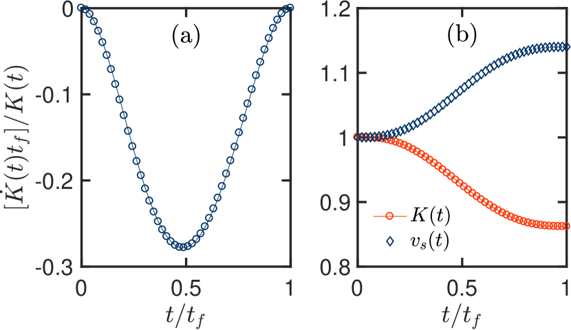
Figure 1: Modulation in time of the amplitude of (a) the counter-diabatic driving Hamiltonian and (b) the Luttinger parameters for an interacting driving protocol following a fifth-order interpolating ansatz with $g_{2}(0)=g_{4}(0)=0$, $g_{2}(t_{f})=2g_{4}(t_{f})=1v_{F}$.

By way of example, let us consider the protocol for the delta interacting potential for the reference Hamiltonian. The modulation of the interaction coupling can be chosen $\tilde{g}_{2/4}(t)=\tilde{g}_{2/4}(0)+[\tilde{g}_{2/4}(t_{f})-\tilde{g}_{2/4}(0)]\mathscr{P}(t/t_{f})$ with a fifth-order polynomial ansatz $\mathscr{P}(t/t_{f})=10(t/t_{f})^{3}-15(t/t_{f})^{4}+6(t/t_{f})^{5}$. The modulation of the Luttinger parameter thus fulfills

$$\frac{\dot{K}(t)}{K(t)}=\frac{\dot{\tilde{g}}_{4}\tilde{g}_{2}-\dot{\tilde{g}}_{2}(2\pi v_{F}+\tilde{g}_{4})}{(2\pi v_{F}+\tilde{g}_{4})^{2}-\tilde{g}^{2}_{2}}.$$

The condition on the driving speed simplifies when $\tilde{g}_{2}(t)=\tilde{g}_{4}(t)=\tilde{g}_{24}(t)$ and $\tilde{g}_{24}(0)=0$ to $t_{f}>L\frac{|\tilde{g}_{24}(t_{f}){\rm max}\dot{\mathscr{P}}(t/t_{f})|}{(2\pi v_{F})^{2}}$. The adiabatic mean energy is equal to the mean energy in the presence of CD. This result allows for preparing an interacting TLL in finite time without nonadiabatic final residual energy. Under CD, the mean energy evolves as the rescaled initial energy Funo et al. (2017)

$$\langle\mathcal{H}(t)\rangle = \frac{v_{s}(t)}{v_{F}}\langle\mathcal{H}(0)\rangle,$$ (20)

with $v_{s}(t)$ given in Eq. (Transitionless Quantum Driving of the Tomonaga-Luttinger Liquid). To this end, it is required that the TLL Hamiltonian parameters are modulated in time as shown in Fig. 1, along a finite-time interaction quench associated with the fifth-order interpolating ansatz. More generally, any long-range interaction may be assumed for $g_{2}(p,t)/(2\pi)$ and $g_{4}(p,t)/(2\pi)$. As we next discuss, an appropriate choice of the potential may facilitate the experimental implementation.

Let us consider the Lorentzian interaction potential

$$V_{2/4}(x-x^{\prime},t)=\frac{\lambda}{\pi}\frac{R_{2/4}(t)}{(x-x^{\prime})^{2}+R^{2}_{2/4}(t)},$$ (21)

that has been previously discussed in the context of the TLL Iucci and Cazalilla (2009); Dóra et al. (2011). In the limit of vanishing interaction range $R_{2/4}(t)\rightarrow 0$, the Lorentzian interaction potential reduces to the contact potential as $V_{2/4}(x-x^{\prime},t)=\lambda\delta(x-x^{\prime})$. We further note that in momentum space, the corresponding interaction strength decays exponentially as $g_{2/4}(p,t)=\lambda\exp(-R_{2/4}(t)|p|)$, denoted by $g_{2/4}$ for short in the following. Let us consider the case $g_{2}=g_{4}=g_{24}=\lambda\exp(-R_{2/4}(t)|p|)$, modifying the potential accordingly

$$\frac{\dot{K}(t)}{2K(t)}=\frac{|p|}{2}\frac{\dot{R}_{2/4}(t)g_{24}}{(2\pi v_{F}+2g_{24})}.$$

The long-range interaction acts as a cutoff parameter where only the momenta $|p|<\frac{1}{R_{2/4}(t)}$ contribute. As a consequence, one can perform a Taylor expansion of the exponential for small $R_{2/4}(t)|p|$. To match with the linear approximation of the Luttinger liquid theory, one can further neglect the higher order terms in $\mathcal{O}(|p|^{2})$ leading to the simplified CD term

$$H_{\rm CD}(t) \approx i\hbar\Delta(t)\sum_{p>0}|p|\left[K_{+}(p)-K_{-}(p)\right]$$ (22)

$$\approx\hbar\Delta(t)\int_{0}^{L}dxdx^{\prime}\frac{\rho_{1}(x)\rho_{-1}(x^{\prime})-\rho_{1}(x^{\prime})\rho_{-1}(x)}{(x^{\prime}-x)},$$

with $\Delta(t)=\frac{1}{2}\frac{\dot{R}_{2/4}(t)\lambda}{(2\pi v_{F}+2\lambda)}$. This Hamiltonian belongs to the Schulz-Shastry model Schulz and Shastry (1998), which can be engineered with gauge potentials Dóra and Moessner (2016), making possible the implementation of STA by CD in the driven TLL.

Conclusion. We have engineered fast-driving shortcut protocols for the nonadiabatic preparation of many-body quantum states in the TLL. To this end, we have identified the auxiliary Hamiltonian controls for transitionelss quantum driving of the TLL, exploiting its analogy with an ensemble of harmonic oscillators with time-dependent mass and frequency. The auxiliary CD Hamiltonian control is the sum of generators of two-mode squeezing in terms of bosonic operators and admits a natural representation upon bosonization. We have specified the CD protocol in terms of the time-dependent TLL parameters and an external potential. The auxiliary CD Hamiltonian could be engineered through a long-range interaction between right and left movers densities that varies according to the form of the $g_{2}$ and $g_{4}$ scattering. Our results open new avenues for engineering shortcuts to adiabaticity and fast quantum control protocols using effective field theories providing an alternative to adiabatic strategies. They should find broad applications in many-particle quantum thermodynamic devices, the study of thermalization, and control of ultracold gases in tight-waveguides and one-dimensional conducting systems.
Acknowledgements.— We are indebted to Baláz Dóra and Per Moosavi for insightful comments. We would like to thank Masahito Ueda, Federico Balducci, Iñigo L. Egusquiza, Apollonas S. Matsoukas Roubeas, Armin Rahmani, and Jing Yang for the interesting discussions. This project was supported by the Luxembourg National Research Fund (FNR Grant No. 16434093). It has received funding from the QuantERA II Joint Programme with co-funding from the European Union’s Horizon 2020 research and innovation programme.

I Details on the derivation of the Tomonaga-Luttinger model

The free Hamiltonian of the TLL can be expressed as Mattis and Lieb (1965)

$$H_{0} = \sum_{p\neq 0}\hbar v_{F}|p|b^{\dagger}(p)b(p)+\frac{\pi v_{F}}{L}(N^{2}+J^{2}),$$ (S1)

with $v_{F}$ the Fermi velocity. The bosonic operators verify the usual commutation rule $[b(p),b^{\dagger}(p^{\prime})]=\delta_{p,p^{\prime}}$ and their link to the densities of right and left movers $\rho_{\pm 1}(p)$ is given in the main text Luttinger (1963); Haldane (1981). Let us now introduce interactions in the model so that the complete Hamiltonian reads $H_{\rm TL}=H_{0}+V$, where the interaction potential takes the form $V=\sum_{i,j=\pm 1}\hat{V}_{ij}$, with

$$\hat{V}_{ij}=\frac{\pi\hbar}{L}\sum_{p>0}\{V_{ij}(p,t)\rho_{i}(-p)\rho_{j}(p)+V_{ij}(-p,t)\rho_{i}(p)\rho_{j}(-p)\}+\frac{\pi\hbar}{L}V_{ij}(0,t)\rho_{i}(0)\rho_{j}(0),$$

and

$$V_{ij}(p,p^{\prime},t) = \frac{1}{L}\int_{0}^{L}dx\int_{0}^{L}dx^{\prime}e^{ipx}V_{ij}(x-x^{\prime},t)e^{ip^{\prime}x^{\prime}},$$

$$V_{ij}(p,p^{\prime},t) = \delta_{p,-p^{\prime}}V_{ij}(p,t).$$

Even parity of the interaction potential is assumed in the following, i.e., $V_{ij}(p,t)=V_{ij}(-p,t)$. In particular, the interaction potential for the backscattering between the right and left movers is denoted $g_{2}(p,t)/(2\pi)=V_{1,-1}(p,t)$, while the forward scattering between right movers and left movers is denoted by $g_{4}(p,t)/(2\pi)=V_{1,1}(p,t)=V_{-1,-1}(p,t)$. Combining the noninteracting and interacting parts leads to the Hamiltonian in the main text (1). The zero-momentum term defined by $C_{0}(t)=\frac{\pi\hbar v_{F}}{L}(N^{2}+J^{2})+\frac{\hbar g_{2}(0,t)}{4L}\left(N^{2}-J^{2}\right)+\frac{\hbar g_{4}(0,t)}{4L}\left(N^{2}+J^{2}\right)$ is gauged away in Eq. (1). Using normal ordering, we denoted by $N=N_{1}+N_{-1}$ the sum of left and right movers and by $J=N_{1}-N_{-1}$ the current operator Mattis (1974).

To establish the field representation of the TLL, consider the field operator with right and left movers $\Psi(x)\approx e^{ik_{F}x}\Psi_{1}(x)+e^{-ik_{F}x}\Psi_{-1}(x)$ Giamarchi (2004). The field can be decomposed according to a phase operator $\phi(x)$ and its conjugated operator $\Pi(x)=\frac{\partial_{x}\theta(x)}{\pi}$, through the bosonization procedure Haldane (1981), yielding in the fermionic case Cazalilla (2004)

$$\Psi^{\dagger}(x)\approx\sqrt{\rho_{0}-\Pi(x)}\sum_{p}e^{i(2p+1)(\pi\rho_{0}x-\theta(x))}e^{-i\phi(x)},$$

where the average density $\rho_{0}$ is related to the Fermi momentum $\pi\rho_{0}=k_{F}$. It is further possible to decompose the fields in the bosonic basis Cazalilla (2004); Giamarchi (2004)

with $\nu$ a cutoff parameter that ensures convergence, in the limit $\nu\to 0$ Haldane (1981). The relation between the field and the bosonic basis is useful for expressing the TLL in its field representation.

II Theory of invariants of motion

A rigorous derivation of the CD term relies on the theory of invariants of motion. Respectively, $I$ is an invariant of motion when $i\hbar\frac{dI(t)}{dt}=i\hbar\frac{\partial I(t)}{\partial t}-[\mathcal{H},I(t)]=0$. Making use of the spectral decomposition of the invariant of motion $I(t)=\sum_{n}\lambda_{n}|\lambda_{n},t\rangle\langle\lambda_{n},t|$ yields the solution to the time-dependent Schrödinger equation with Hamiltonian $\mathcal{H}$ in the form Lohe (2008) $|\Psi_{t}\rangle=\exp\left(i\int_{0}^{t}\kappa_{n}(s)ds\right)|\lambda_{n},t\rangle,$ with $\kappa_{n}(s)=\langle\lambda_{n},s|i\frac{\partial}{\partial t}-\frac{\mathcal{H}}{\hbar}|\lambda_{n},s\rangle$. One can construct a time-dependent invariant $I=QI^{0}Q^{\dagger}$ using a time-independent operator $I^{0}$ and a unitary time-evolution operator $Q$. The corresponding Hamiltonian is

$$\mathcal{H}(t)=F(I,t)+i\hbar\frac{\partial Q}{\partial t}Q^{\dagger},$$ (S2)

where $F(I,t)=I/\sigma^{2}_{t}$ and $\sigma_{t}$ a scalar time-dependent function. The dynamical phase can be expressed by direct substitution of $|\Psi_{t}\rangle$ in the Schrödinger equation with Hamiltonian (S2), one obtains the phase $\kappa_{n}(s)=-\frac{1}{\hbar}\langle\lambda_{n},s|F(I,t)|\lambda_{n},s\rangle$.

III Counterdiabatic controls for the quantum oscillator with driven mass and frequency

As the TLL is analogous to an ensemble of quantum harmonic oscillators with time-dependent mass and frequency, it is useful to study the counter-diabatic driving in the latter case. We make use of Lohe’s solution of the time-dependent Schrödinger equation $i\hbar\frac{d|\Psi(t)\rangle}{dt}=H|\Psi(t)\rangle$ with Hamiltonian Lohe (2008)

$$H(t)=\frac{\gamma^{2}}{2m_{0}\sigma^{2}_{t}}p^{2}+\frac{1}{2}m_{0}\frac{\omega^{2}_{0}}{\sigma^{2}_{t}\gamma^{2}}x^{2}+\frac{\dot{\gamma}}{2\gamma}\{x,p\}.$$ (S3)

Consider the $n$-th eigenstate $\phi_{n}$ of the (time-independent) initial harmonic oscillator $\hat{H}=\frac{p^{2}}{2m_{0}}+\frac{1}{2}m_{0}\omega^{2}_{0}x^{2}$ with associated eigenvalue $E_{n}(0)$. Its evolution, governed by (S3), reads

$$|\Psi_{n}(t)\rangle=\gamma^{-1/2}\exp\left(-\frac{i}{\hbar}\int_{t_{0}}^{t}\frac{E_{n}(0)ds}{\sigma^{2}_{s}}\right)\phi_{n}\left(\frac{x}{\gamma},0\right).$$

We identify the time-dependent mass $m(t)=\frac{m_{0}\sigma^{2}_{t}}{\gamma^{2}}$ and frequency $\omega^{2}(t)=\frac{\omega^{2}_{0}}{\sigma^{4}_{t}}$, so that $\gamma=\sqrt{\frac{m_{0}\omega_{0}}{m(t)\omega(t)}}$ and $\sigma_{t}=\sqrt{\frac{\omega_{0}}{\omega(t)}}$. The Hamiltonian (S3) takes then the form

$$H(t)=\frac{1}{2m(t)}p^{2}+\frac{1}{2}m(t)\omega^{2}(t)x^{2}-\frac{1}{4}\left(\frac{\dot{m}(t)}{m(t)}+\frac{\dot{\omega}(t)}{\omega(t)}\right)\{x,p\}.$$

Thus, one can identify the reference Hamiltonian to be $H_{0}(t)=\frac{1}{2m(t)}p^{2}+\frac{1}{2}m(t)\omega^{2}(t)x^{2}$ and the CD term as $H_{\rm CD}(t)=-\frac{1}{4}\left(\frac{\dot{m}(t)}{m(t)}+\frac{\dot{\omega}(t)}{\omega(t)}\right)\{x,p\}$, generalizing the well-known result for with time-dependent frequency and constant mass Muga et al. (2010). The latter is recovered for $\sigma_{t}=\gamma$ Torrontegui et al. (2013). The quantum harmonic oscillator algebra can be expressed as a function of the $SU(1,1)$ generators so that $\hat{x}=\sqrt{\frac{\hbar}{2m\omega}}(a^{\dagger}+a)$ and $\hat{p}=i\sqrt{\frac{\hbar m\omega}{2}}(a^{\dagger}-a)$, with $a$ and $a^{\dagger}$ being the canonical annihilation and creation operators, verifying the commutation rule $[a,a^{\dagger}]=1$. We define $J_{+}=\frac{1}{2}a^{\dagger 2}$, $J_{-}=\frac{1}{2}a^{2}$, and $J_{0}=\frac{1}{4}(a^{\dagger}a+aa^{\dagger})$, that verify the commutation rules $[J_{0},J_{\pm}]=\pm J_{\pm}$ and $[J_{-},J_{+}]=2J_{0}$. In terms of them, $\hat{x}^{2}=\frac{\hbar}{m_{0}\omega_{0}}(2J_{0}+J_{+}+J_{-})$, $\hat{p}^{2}=\hbar m_{0}\omega_{0}(2J_{0}-J_{+}-J_{-})$ and $\{x,p\}=i\hbar(a^{\dagger 2}-a^{2})=2i\hbar(J_{+}-J_{-})$.

By analogy, one can introduce the momentum-dependent harmonic oscillator. One can introduce the momentum-dependent pseudo-position and momentum operators

$$X_{p} =\sqrt{\frac{\hbar}{2\omega_{0p}}}[b^{\dagger}(p)+b(-p)],$$ (S6)

$$X_{-p} =\sqrt{\frac{\hbar}{2\omega_{0p}}}[b^{\dagger}(-p)+b(p)].$$ (S7)

They are not Hermitian, as $X^{\dagger}_{p}=X_{-p}$. However, their product is, as $(X_{p}X_{-p})^{\dagger}=X^{\dagger}_{-p}X^{\dagger}_{p}=X_{p}X_{-p}$ and

$$X_{p}X_{-p}=\frac{\hbar}{2\omega_{0p}}[2K_{0}(p)+K_{+}(p)+K_{-}(p)].$$ (S8)

Similarly, one can introduce $P_{p}=i\sqrt{\frac{\hbar\omega_{0}}{2}}[b^{\dagger}(p)-b(-p)]$ so that

$$P_{p}P_{-p}=\frac{\hbar\omega_{0p}}{2}[2K_{0}(p)-(K_{+}(p)+K_{-}(p))].$$ (S9)

One can use these operators to express the TLL Hamiltonian as an ensemble of harmonic oscillators with time-dependent mass and frequency (Transitionless Quantum Driving of the Tomonaga-Luttinger Liquid).

IV Mean Energy under counterdiabatic driving

The nonadiabatic mean energy in the driven TLL under CD reads

$$\langle\Psi(t)|\mathcal{H}(t)|\Psi(t)\rangle = \langle\Psi(0)|Q^{\dagger}\left(Q\frac{I^{0}}{\sigma^{2}_{t}}Q^{\dagger}+i\hbar\frac{\partial Q}{\partial t}Q^{\dagger}\right)Q|\Psi(0)\rangle$$ (S10)

$$= \langle\Psi(0)|\frac{I^{0}}{\sigma^{2}_{t}}|\Psi(0)\rangle+i\hbar\langle\Psi(0)|Q^{\dagger}\frac{\partial Q}{\partial t}|\Psi(0)\rangle,$$

However, the explicit evaluation shows that

$$i\hbar Q^{\dagger}\frac{\partial Q}{\partial t} = i\hbar\sum_{p\neq 0}\frac{\dot{\gamma_{p}}}{2\gamma_{p}}[K_{+}(p)-K_{-}(p)].$$ (S11)

As a result,

$$\langle\Psi(t)|\mathcal{H}(t)|\Psi(t)\rangle = \langle\Psi(0)|\frac{I^{0}}{\sigma^{2}_{t}}|\Psi(0)\rangle+i\hbar\sum_{p\neq 0}\frac{\dot{\gamma_{p}}}{2\gamma_{p}}\langle\Psi(0)|[K_{+}(p)-K_{-}(p)]|\Psi(0)\rangle$$ (S12)

$$= \langle\Psi(0)|\frac{I^{0}}{\sigma^{2}_{t}}|\Psi(0)\rangle.$$ (S13)

In short, the nonadiabatic mean energy along the CD protocol can be expressed in terms of its initial value and the scaling function $\sigma_{t}$.

V Implementation of the counter-diabatic driving term

The CD Hamiltonian can be conveniently written as

$$H_{\rm CD}(t) = -i\hbar\sum_{p>0}\frac{\dot{K}}{2K}[b(p)b(-p)-b^{\dagger}(p)b^{\dagger}(-p)]$$ (S14)

$$= -i\hbar\sum_{p>0}\frac{\dot{K}}{2K}\frac{2\pi}{Lp}\Big{(}\rho_{1}(-p)\rho_{-1}(p)-\rho_{1}(p)\rho_{-1}(-p)\Big{)}$$ (S15)

$$= -i\hbar\sum_{p>0}\frac{\dot{K}}{2K}\frac{2\pi}{Lp}\int_{0}^{L}dx\int_{0}^{L}dx^{\prime}\Big{(}\rho_{1}(x)\rho_{-1}(x^{\prime})-\rho_{1}(x^{\prime})\rho_{-1}(x)\Big{)}e^{ip(x^{\prime}-x)}.$$ (S16)

Using the quantization of the momentum $p=\frac{2\pi}{L}n$ with $n\in\mathbbm{N}^{*}$, one can write the sum

$$\mathcal{S}(x^{\prime}-x)=\sum_{n=1}^{\infty}\frac{e^{i\frac{2\pi}{L}n(x^{\prime}-x)}}{n}.$$ (S17)

For the special values $x=x^{\prime}$ and $|x^{\prime}-x|=L$, the infinite sum diverges; $\mathcal{S}(x^{\prime}-x)\to+\infty$. We would like to show that at these specific points, the function $\mathcal{S}(x^{\prime}-x)$ can be approximated as a delta function. Given a test function $f(x)$, as a generalized distribution, the delta function satisfies $\int dxf(x)\delta(x)=f(0)$, along with the normalization condition $\int dx\delta(x)=1$. We first verify that $\mathcal{S}(r)$ is a normalizable function on its domain of definition $r\in[-L,L]$. Indeed,

$$\int_{-L}^{L}dr\mathcal{S}(r)=\frac{1}{i\frac{2\pi}{L}}\left(\sum_{n=1}^{\infty}\frac{e^{i2\pi n}}{n^{2}}-\frac{e^{-i2\pi n}}{n^{2}}\right)=\frac{L}{\pi}\sum_{n=1}^{\infty}\frac{\sin(2\pi n)}{n^{2}}.$$ (S18)

Furthermore, this last series is bounded in absolute value by a convergent series

$$\left|\sum_{n=1}^{\infty}\frac{\sin(2\pi n)}{n^{2}}\right|\leq\sum_{n=1}^{\infty}\frac{1}{n^{2}}.$$ (S19)

Using the property of absolute convergence, the function $\mathcal{S}(r)$ is then normalizable on $[-L,L]$. As a consequence, we can approximate $S(r)$ to mimic a delta function at the special values $x=x^{\prime}$ and $|x-x^{\prime}|=L$. Note, however, that outside these points, the function is not equal to zero, so we need to add a supplementary contribution to the points $x\neq x^{\prime}$. Overall, we can write $\mathcal{S}(x^{\prime}-x)$ as a function of its different contributions $\mathcal{S}(0)+\mathcal{S}(L)+\mathcal{S}(-L)+\mathcal{S}(x^{\prime}-x)_{x^{\prime}-x\neq\{0,L,-L\}}=\delta(x^{\prime}-x)+\delta(x^{\prime}-x-L)+\delta(x^{\prime}-x+L)+\mathcal{S}(x^{\prime}-x)_{x^{\prime}-x\neq\{0,L,-L\}}$. Furthermore, one can use the Euler’s formula to decompose the exponential

$$\sum_{n=1}^{\infty}\frac{e^{i\frac{2\pi}{L}n(x^{\prime}-x)}}{n}=\sum_{n=1}^{\infty}\frac{\cos[\frac{2\pi}{L}n(x^{\prime}-x)]}{n}+i\sum_{n=1}^{\infty}\frac{\sin[\frac{2\pi}{L}n(x^{\prime}-x)]}{n}.$$ (S20)

It is then useful to notice the formula Zwillinger (2014) for $a\in(0,2\pi)$

$$\sum_{n=1}^{\infty}\frac{\sin(na)}{n}=\frac{\pi-a}{2}.$$ (S21)

As the cosine is an even function, its contribution to the integral vanishes, and one is left with

$$H_{\rm CD}(t) = -i\hbar\frac{\dot{K}}{2K}\int_{0}^{L}dxdx^{\prime}\Big{[}\rho_{1}(x)\rho_{-1}(x^{\prime})-\rho_{1}(x^{\prime})\rho_{-1}(x)\Big{]}\Big{[}\delta(x^{\prime}-x)+\delta(x^{\prime}-x-L)+\delta(x^{\prime}-x+L)+\frac{\pi-\frac{2\pi(x^{\prime}-x)}{L}}{2}\Big{]}.$$

Using again that even functions do not contribute to the integral, one finds the expression quoted in the main text.

It is interesting to look at the effect of long-range interactions on the CD Hamiltonian form. An alternative implementation is found in using the Lorentzian potential for the long-range interaction

$$H_{\rm CD}(t) = -i\hbar\Delta(t)\sum_{p>0}|p|[K_{-}(p)-K_{+}(p)],$$ (S23)

$$= -i\hbar\Delta(t)\sum_{p>0}\frac{2\pi}{L}[\rho_{1}(-p)\rho_{-1}(p)-\rho_{1}(p)\rho_{-1}(-p)]$$ (S24)

$$= -i\hbar\Delta(t)\frac{2\pi}{L}\int_{0}^{L}dx\int_{0}^{L}dx^{\prime}[\rho_{1}(x)\rho_{-1}(x^{\prime})-\rho_{1}(x^{\prime})\rho_{-1}(x)]\sum_{p>0}\frac{e^{ip(x^{\prime}-x)}}{2}$$ (S25)

$$= -i\hbar\Delta(t)\frac{2\pi}{L}\int_{0}^{L}dx\int_{0}^{L}dx^{\prime}[\rho_{1}(x)\rho_{-1}(x^{\prime})-\rho_{1}(x^{\prime})\rho_{-1}(x)]\sum_{p>0}\frac{\left(e^{ip(x^{\prime}-x)}-e^{-ip(x^{\prime}-x)}\right)}{2}$$ (S26)

$$= -i\hbar\Delta(t)\frac{2\pi}{L}\int_{0}^{L}dx\int_{0}^{L}dx^{\prime}[\rho_{1}(x)\rho_{-1}(x^{\prime})-\rho_{1}(x^{\prime})\rho_{-1}(x)]\ \sum_{n=1}^{\infty}\frac{\left(e^{i\frac{2\pi n}{L}(x^{\prime}-x)}-e^{-i\frac{2\pi n}{L}(x^{\prime}-x)}\right)}{2}$$ (S27)

$$= \hbar\Delta(t)\frac{\pi}{L}\int_{0}^{L}dx\int_{0}^{L}dx^{\prime}[\rho_{1}(x)\rho_{-1}(x^{\prime})-\rho_{1}(x^{\prime})\rho_{-1}(x)]\frac{1}{\tan[\frac{\pi}{L}(x^{\prime}-x)]}$$ (S28)

$$\approx -\hbar\Delta(t)\int_{0}^{L}dx\int_{0}^{L}dx^{\prime}[\rho_{1}(x)\rho_{-1}(x^{\prime})-\rho_{1}(x^{\prime})\rho_{-1}(x)]\left[\frac{1}{(x-x^{\prime})}-\frac{\pi^{2}}{3L^{2}}(x-x^{\prime})+\mathcal{O}(L^{-4})\right],$$ (S29)

leading to the result presented in the main text.

VI Spectrum through the Bogoliubov transformation

The Tomonaga-Luttinger liquid with $\rm CD$ Hamilontian is written as

$$\mathcal{H}(t) = \hbar\sum_{p\neq 0}\omega_{\rm CD}(p,t)K_{0}(p)+\hbar\sum_{p\neq 0}\alpha(t)K_{+}(p)+\hbar\sum_{p\neq 0}\alpha^{*}(t)K_{-}(p),$$ (S30)

$$\alpha(t) = \frac{g_{\rm CD}(p,t)}{2}+i\frac{\dot{\gamma_{p}}}{2\gamma_{p}}.$$ (S31)

One can set

$$b(p)=ud(p)+vd^{\dagger}(-p).$$ (S32)

The bosonic commutation relation $[b(p),b^{\dagger}(p^{\prime})]=\delta_{p,p^{\prime}}$ enforces the condition

$$|v|^{2}-|u|^{2}=1,$$ (S33)

leading to the parametrization

$$u = e^{i\theta_{1}}\cosh(r),$$ (S34)

$$v = e^{i\theta_{2}}\sinh(r).$$ (S35)

In the new basis, the Hamiltonian becomes

$$\mathcal{H}(t) = \hbar\sum_{p\neq 0}\left[\frac{\omega_{\rm CD}(p,t)}{2}(|u|^{2}+|v|^{2})+\alpha u^{*}v^{*}+\alpha^{*}uv\right]d^{\dagger}(p)d(p)$$ (S36)

$$+ \hbar\sum_{p\neq 0}\left[\omega_{\rm CD}(p,t)uv^{*}+\alpha(v^{*})^{2}+\alpha^{*}u^{2}\right]d(-p)d(p)$$ (S37)

$$+ \hbar\sum_{p\neq 0}\left[\frac{\omega_{\rm CD}(p,t)}{2}(|u|^{2}+|v|^{2})+\alpha v^{*}u^{*}+\alpha^{*}uv\right]d(-p)d^{\dagger}(-p)$$

$$+ \hbar\sum_{p\neq 0}\left[\omega_{\rm CD}(p,t)u^{*}v+\alpha(u^{*})^{2}+\alpha^{*}v^{2}\right]d^{\dagger}(p)d^{\dagger}(-p).$$

The diagonalization condition is given by

$$0=\omega_{\rm CD}(p,t)e^{i(\theta_{2}-\theta_{1})}\frac{1}{2}\sinh(2r)+|\alpha|e^{i\phi_{\alpha}}e^{-2i\theta_{1}}\cosh^{2}(r)+|\alpha|e^{-i\phi_{\alpha}}e^{2i\theta_{2}}\sinh^{2}(r),$$ (S40)

with $\theta_{1}=\theta_{2}$ with $\theta_{1}=\phi_{\alpha}/2$ and

$$\tanh(2r)=-\frac{2|\alpha|}{\omega_{\rm CD}(p,t)}.$$ (S41)

The previous relation is obeyed only if $\left|2|\alpha|/\omega_{\rm CD}(p,t)\right|<1$. The spectrum can be written as

$$\epsilon(p,t) = \omega_{\rm CD}(p,t){\rm sech}(2r)=\sqrt{\omega^{2}_{\rm CD}(p,t)-g^{2}_{\rm CD}(p,t)-\left(\frac{\dot{\gamma_{p}}}{\gamma_{p}}\right)^{2}}$$ (S42)

$$= \sqrt{\frac{\omega^{2}_{0p}}{\sigma^{4}_{t}}-\left(\frac{\dot{\gamma_{p}}}{\gamma_{p}}\right)^{2}}$$ (S43)

$$= \sqrt{v^{2}_{s}|p|^{2}-\left(\frac{\dot{K}}{2K}\right)^{2}},$$ (S44)

where we used $\cosh[{\rm arctanh}(x)]=\frac{1}{\sqrt{1-x^{2}}}$ for $|x|<1$.

VII Stability criteria for the TLL

For the TLL to be stable, the energy spectrum should be bounded from below

$$\sqrt{v^{2}_{s}(t)|p|^{2}-\left(\frac{\dot{K}(t)}{2K(t)}\right)^{2}}>0.$$ (S45)

Even though small momenta are more prone to lead to an imaginary spectrum in the presence of CD, a small enough amplitude for the CD Hamiltonian may not lead to a divergence of the dynamics. Indeed, the minimal value for the momentum is $p=\frac{2\pi}{L}$. Hence,

$$\left|v_{s}(t)\left(\frac{2\pi}{L}\right)\right|>\left|\frac{\dot{K}(t)}{2K(t)}\right|,$$ (S46)

sets a bound on the speed at which the process can be performed for finite-size systems. In the case of the delta-interacting potential $\tilde{g}_{2}(t)=\tilde{g}_{4}(t)=\tilde{g}_{24}(t)$, the condition simplifies to

$$\left|\frac{v_{F}[\dot{\tilde{g}}_{24}(t)/2\pi]}{v^{3}_{s}(t)}\right|=\left|\frac{\dot{v}_{s}(t)}{v^{2}_{s}(t)}\right|<\frac{2\pi}{L}.$$ (S47)

This is reminiscent of the adiabatic condition for the time-dependent harmonic oscillator established by Lewis and Riesenfeld Lewis and Riesenfeld (1969b)

$$\left|\frac{\dot{\Omega}(p,t)}{\Omega^{2}(p,t)}\right|=\left|\frac{\dot{v}_{s}(t)}{v^{2}_{s}(t)|p|}\right|\ll 1.$$ (S48)

Thus, the same control parameter governs the onset of adiabaticity under slow driving and the breaking of the TLL description in a STA by CD. The driving regime of interest for the CD protocol spans the range of driving speeds between these two limits. We explore this regime considering the previous experimental implementation of the TLL in ultracold atoms Yang et al. (2017); Gluza et al. (2022); Tajik et al. (2023). In Yang et al. (2017), the authors measured a sound velocity $v_{s}\approx 2.21\ {\rm\mu m/ms}$ and considered a system size $L=10-100\ {\rm\mu m}$. In Tajik et al. (2023), the authors considered $L\approx 50\ {\rm\mu m}$ and ${v}_{s}\approx 2.04\ {\rm\mu m/ms}$. By dimensional analysis $|\dot{v}_{s}/v^{2}_{s}|\approx 1/(t_{f}v_{s})$, and the quench time needs to be larger than $t_{f}>\frac{L}{2\pi v_{s}}\approx 3.90\ {\rm ms}$. The adiabatic quench has to be very large compared to this time so that the regime of interest of the counterdiabatic protocol is between $3.9{\rm ms}$ and $39{\rm ms}$ for the given experimental values. The sound velocity was computed with the formula ${v}_{s}=\sqrt{g_{\rm 1D}{n}_{\rm 1D}/m}$ Tajik et al. (2023) with the $1D$ interaction strength $g_{\rm 1D}=\hbar\omega_{\perp}a_{s}\frac{2+3a_{s}n_{\rm 1D}}{1+2a_{s}n_{\rm 1D}}$, the three dimensional scattering length $a_{s}=5.2\ {\rm nm}$, the mass $m=1.44\times 10^{-25}\ {\rm kg}$ of the ${}^{87}{\rm Rb}$ atom, the transverse trapping frequency $\omega_{\perp}=2\pi\times 1.4\ {\rm kHz}$, and the density $n_{\rm 1D}\approx 70\ {\rm\mu m}^{-1}$.