Classical origins of Landau-incompatible transitions
Abstract
Continuous phase transitions where symmetry is spontaneously broken are ubiquitous in physics and often found between ‘Landau-compatible’ phases where residual symmetries of one phase are a subset of the other. However, continuous ‘deconfined quantum critical’ transitions between Landau-incompatible symmetry-breaking phases are known to exist in certain quantum systems, often with anomalous microscopic symmetries. In this paper, we investigate the need for such special conditions. We show that Landau-incompatible transitions can be found in a family of well-known classical statistical mechanical models with anomaly-free on-site microscopic symmetries, introduced by José, Kadanoff, Kirkpatick and Nelson (Phys. Rev. B 16, 1217). The models are labeled by a positive integer and constructed by a deformation of the 2d classical XY model, defined on any lattice, with an on-site potential that preserves a discrete -fold spin rotation and reflection symmetry. For a range of temperatures, even models exhibit two Landau-incompatible partial symmetry-breaking phases and a direct transition between them for . Characteristic features of Landau-incompatible transitions are easily seen, such as enhanced symmetries and melting of charged defects. For odd , and corresponding temperature ranges, two regions of a single partial symmetry-breaking phase are obtained, split by a stable ‘unnecessary critical’ line. We present quantum models with anomaly-free symmetries that also exhibit similar phase diagrams.
Spontaneous symmetry breaking (SSB) underpins several important physical phenomena, from the development of long-range orders in matter to endowing mass to fundamental particles [1]. The simplest setting for SSB is when a phase of matter, classical or quantum, with a vacuum invariant under a symmetry group undergoes a phase transition to produce multiple vacua, each of which preserves only a subset of the original symmetries . If such a phase transition is continuous, it can be described within the Landau-Ginzburg-Wilson-Fisher (LGWF) framework using a local order parameter field. About twenty years ago, the nature of exotic direct transitions between incompatible SSB quantum phases, where the vacuum symmetries of neither phase could be identified as a subset of the other, was investigated in two-dimensional quantum systems [2]. Although such transitions had appeared in earlier studies [3], Ref. [2] recognized the importance of the fact that they could not be framed within the LGWF paradigm in terms of order parameter fields. Instead, they were naturally formulated using gauge fields, which are hidden from sight in the ordered phases but appear at the transition. This prompted the moniker ‘deconfined quantum criticality’ (DQC) [2, 4].

What physical settings can give rise to such Landau-incompatible transitions? Descriptions using non-linear sigma models [5] and low-dimensional examples [6, 7] have made it clear that deconfined gauge fields are not necessary. However, in most known examples, DQC appears in quantum systems when microscopic symmetries are anomalous [8, 9]. In this paper, we show that most of these conditions are not necessary and Landau-incompatible transitions can, in fact, be found even in ordinary classical statistical mechanical systems with anomaly-free symmetries. We demonstrate this using a well known family of models introduced by José, Kadanoff, Kirkpatrick and Nelson (JKKN) [10] obtained by perturbing the 2d classical XY model by on-site potentials labeled by a positive integer . For even , the phase diagram consists of a direct Landau-incompatible phase transition between two partial symmetry-breaking phases. This transition displays all notable characteristics of DQC, including the appearance of an enhanced symmetry that rotates between the order parameters of the Landau-incompatible phases and the melting of charged defects. Interestingly, neutral defects and charges also independently exist and can condense to produce Landau-compatible phase transitions. For odd , we find the appearance of an exotic second-order ‘unnecessary critical’ line separating two regions of single phase that does not represent a genuine phase transition [11, 12] but is nevertheless stable. To our knowledge, this is the first case of unnecessary criticality identified in a classical model. Finally, we also present a family of quantum models with anomaly-free symmetries that exhibit similar phase diagrams. Altogether, our results show that exotic transitions beyond the LGWF paradigm are more abundant than previously believed.
Models and phase diagram:

Let us consider the JKKN model [10] which is a classical statistical mechanical system of planar rotors , located on the vertices of any two-dimensional lattice with Hamiltonian
| (1) |
here labels the vertices and the edges of the lattice. The relevant symmetry group of the system is generated by a rotation and a reflection acting as
| (2) |
The two generators do not commute but satisfy
| (3) |
and thus form the non-abelian dihedral group . To determine the phase diagram of Eq. 1, we will study the partition function
| (4) |
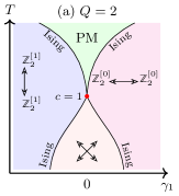
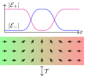
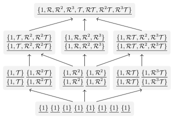
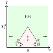
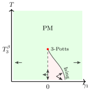
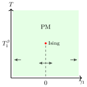
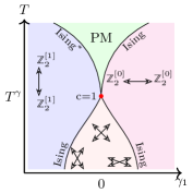
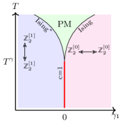
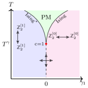
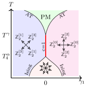
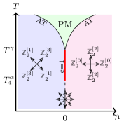
varying and the temperature while keeping all other terms fixed, the most important being . We will be interested in the phase diagrams close to . This is shown schematically in Fig. 1 for and all kept small (see Appendix B). Let us summarize its main aspects [10, 13]:
-
1.
At low temperatures and , we obtain an ordered phase with full symmetry breaking (abbreviated f-SSB) and vacua. For , this becomes a first-order line separating partial SSB regions described below (see Appendix B).
-
2.
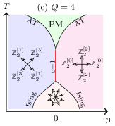
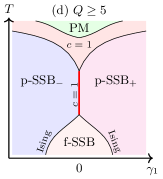
For a range of intermediate temperatures, we obtain two regions with partial SSB (abbreviated p-SSB± for and respectively), each containing vacua. These are separated from the f-SSB phase by an Ising transition for any [14]. For even , p-SSB± represent two distinct Landau-incompatible SSB phases, whereas for odd , they correspond to the same phase.
- 3.
-
4.
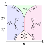
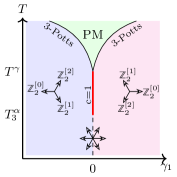
At high temperatures, we get a disordered paramagnetic phase (PM) that restores all symmetries. This is separated from the partial SSB phases by a direct transition belonging to the Ising, 3-state Potts and Ashkin-Teller universality classes (or their symmetry-enriched variants [15, 16, 17]) for respectively [13], and by an intermediate gapless phase for [10].
The phase diagrams in Fig. 1 are determined by replacing Eq. 1 by an effective gaussian continuum theory [10, 13] via a duality transformation á la Villain [18]
| (5) |
and keeping track of the relevance (in the renormalization group sense) of the scaling operators (see Appendix B for details). Recall that a scaling operator is relevant when its scaling dimension is smaller than the spatial dimension (two in our case) for such classical statistical mechanical systems [19]. The term is included as a regulator in the Villain procedure. While the exact relationship between the scaling dimensions and the microscopic parameters cannot be determined exactly, close to the gaussian fixed point, we have the following.
| (6) |
Eq. 6 tells us that for , there exists a regime where is the only relevant symmetry-allowed operator. Tuning this away by setting produces a critical state corresponding to the Landau-incompatible transition or unnecessary critical line. Furthermore, we expect to increase with to obtain the disordered phase driven by at high temperature.
Important parts of the phase diagrams in Fig. 1 have already been explored in previous work (see Refs.[10, 13]). Our main focus will be on symmetry properties, Landau-(in)compatible nature of transitions, unnecessary criticality, and the distinction between even and odd . These aspects have not previously been investigated, to the best of our knowledge.
Residual symmetries, Landau (in)compatibility: Let us understand the nature of the partial symmetry breaking regions (p-SSB±) which are realized for and respectively at intermediate temperatures, where the only relevant operator in Eq. 5 is . Both have vacua characterized by the vacuum expectation value with
| (7) |
The symmetries shown in Eq. 2 act on the vacua as
| (8) |
Since both regions have the same number of vacua, only two possibilities exist: (i) the regions are distinct phases that are Landau-incompatible or (ii) they correspond to the same phase (see Appendix A for more details). To clarify which, we need to determine the residual symmetries of each vacuum in both regions. Using Eq. 8, we see that the vacua transform into each other under the discrete rotation symmetry but preserve a specific subgroup generated by reflection followed by a certain number of rotations . To distinguish between various groups, we define the following notation:
| (9) |
with identified. Using these, we get
| (10) |
Fig. 1 lists the residual symmetries for representative values of . For even , these are distinct for p-SSB± and the vacua are invariant under followed by even (odd) rotations for . The p-SSB± phases are detected, respectively, by the following order parameters,
| (11) |
There is no way to identify the residual symmetries of the vacua of one phase with subsets of those of the other, and therefore the phases are distinct and Landau-incompatible. We see the advertised direct transition between them along for a range of temperatures with continuous critical exponents described by the gaussian CFT that Eq. 5 flows to.
For odd on the other hand, the residual symmetries for both p-SSB± are identical and detected by the same order parameter,
| (12) |
The vacua on both sides can be identified as follows
| (13) |
This leads to the conclusion that both belong to the same phase and that there should exist a path where the vacua and can be smoothly connected without encountering a phase transition. This is seen most clearly for when, in fact, p-SSB± are smoothly connected to the trivial phase and each other (see Appendix B). Thus, for odd , the critical line along represents ‘unnecessary criticality’ [11, 12] which does not correspond to a genuine transition separating distinct phases but is nevertheless stable and reached by tuning a single relevant parameter. To the best of our knowledge all known instances of unnecessary criticality [20, 21, 12, 22, 11, 23] have been observed in quantum mechanical systems in a topological ‘failed SPT’ context [24, 25, 26] and ours is the first example in classical symmetry-breaking setting.
For completeness, let us consider the remaining phases and transitions in Fig. 1. The full symmetry breaking phase (f-SSB) appears when becomes relevant along the line at low temperatures, this has vacua characterized by with
| (14) |
deep in the phase and detected by the order parameter . The symmetries in Eq. 2 transform the vacua into each other as follows (with identified) as
| (15) |
From Eq. 15, we see that the only residual symmetry for all vacua is the trivial subgroup . It is easy to verify that the transition between p-SSB± and f-SSB is Landau-compatible and belongs to the Ising universality class [17, 14]. Finally, at large values of along the line, all symmetries are restored when becomes relevant in Eq. 5 to produce a disordered paramagnet (PM). For , the transition between the p-SSB± and the PM is direct and also Landau-compatible whose universality class depends on [17, 13] as shown in Fig. 1.
Enhanced symmetries, charged defects:
We now study two prominent aspects of Landau-incompatible deconfined critical transitions. The first is the appearance of enhanced symmetries involving rotations between order-parameters of the phases that the DQC line separates. This is readily seen for our model. Notice that along , the symmetry is enhanced to generated by and an enhanced fold rotation
| (16) |
For even , this transforms the order parameters for the Landau-incompatible pSSB± phases shown in Eq. 11, into each other.
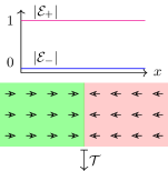
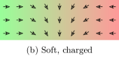
The second aspect is the physical picture for the onset of DQC being the proliferation of charged defects that prevents the restoration of symmetries [4]. This is also clearly seen in our model. In the vicinity of the DQC transition along , the relevant excitations are smooth interpolations between vacua with the same residual symmetries. The domain walls resulting from this interpolation are charged under the residual symmetry. For illustration, let us focus on where, for even , two of the vacua of the resulting p-SSB+ phase are with the same residual symmetry, . If we create a smooth interpolation between these vacua as shown in Fig. 3(b), we see that the resulting domain wall transforms under and thus carries charge. Furthermore, by evaluating the order parameter on this configuration, we see that it vanishes on the domain wall, whereas the order parameter , which vanishes everywhere else, becomes non-zero at the domain wall. Thus, upon melting the p-SSB+ domain walls, we get p-SSB- order!
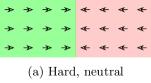
Other interesting features are revealed by understanding the mechanisms of the other transitions out of the p-SSB phases. In addition to the charged domain walls, we also have ordinary excitations charged under the residual symmetries corresponding to local deviation from the minima. Condensing these excitations results in further symmetry breaking and the Ising transition into the f-SSB phase. On the other hand, if we go to the limit, the excitations are ‘hard’ domain walls as shown in Fig. 3(a). These do not transform under the residual symmetries, and their condensation by increasing temperature restores all symmetries. As we reduce , we see that the neutral, hard domain walls soften by absorbing charge, as shown in Fig. 3 and eventually melt to trigger the DQC transition. An analogous charge-binding transition and associated exotic critical phenomena in a 2d classical model were investigated in Refs [27, 28].
Quantum models: All important parts of the phase diagrams of Eq. 1 are qualitatively reproduced by the ground states of the following quantum Hamiltonians
| (17) | ||||
are standard spin half angular momentum operators, is the XXZ spin chain and is a term that favours SSB. Both choices of favour disordered paramagnets that preserve all symmetries, but the second choice also produces a symmetry-protected topological (SPT) phase for one of the signs of . The symmetries in Eq. 2 are generated by
| (18) |
whereas is a time-reversal symmetry generated by complex conjugation in the basis. This model can be bosonized to get the same field theory as in Eq. 5 for , up to renormalization of coupling constants.
The role of anomalies: Deconfined criticality is sometimes associated to the microscopic symmetries being realized anomalously [4] either on the ultraviolet [3, 29, 30, 31] or infrared [8, 9, 32] degrees of freedom 111Note that this prejudice is not universally held, as evidenced by the search for a direct DQC transition between the Néel and valence-bond solid (VBS) phases on the honeycomb lattice [37, 9] which is not constrained by the LSM theorem. However, recent work [40] has indicated that this transition may in fact not exist. Our work proves that even if this particular DQC is not present in the honeycomb lattice, there is no fundamental obstruction to observing Landau-incompatible transitions on the honeycomb or other LSM-trivial lattices.. Anomalies are non-trivial manifestations of symmetries that forbid a strictly on-site representation [34], present an obstruction to gauging [35, 36] and disallow a trivial symmetry-preserving phase [9, 31]. Common settings for anomalies and DQC are systems constrained by Lieb-Schultz-Mattis (LSM) conditions [3, 29, 31, 30] or on the boundaries of symmetry-protected topological phases [34, 7].
The microscopic symmetries in Eq. 2 for both classical and quantum Hamiltonians in Eqs. 1 and 17 are anomaly-free at all scales. This is verified by the presence of the symmetry-allowed operator in Eq. 5 which produces a trivial phase — a sufficient condition for the absence of anomalies. However, when is irrelevant, a new continuous rotation symmetry emerges which has a well-known mixed anomaly with the microscopic symmetry [9, 36]. We may say that this microscopic-emergent mixed anomaly endows stability to the exotic transitions. A case was made for a possible transition between the Néel to valence-bond solid (VBS) phases on the honeycomb lattice [37] being stabilized by a similar anomaly in Ref [9]. However, some care is warranted. In fact, the critical Ising model, which is the archetypal Landau-compatible transition, also has a mixed anomaly between the microscopic Ising symmetry and the emergent Kramers-Wannier symmetry [38]. The key difference is that the microscopic-emergent mixed anomaly of the critical Ising model is explicitly broken by relevant operators, whereas the same is broken by irrelevant operators in our model. In summary, although all microscopic symmetries are anomaly-free, a mixed anomaly between microscopic and emergent symmetries that is preserved by all relevant operators can stabilize both Landau-incompatible and unnecessary critical transitions. It is unclear if this is a necessary condition for Landau-incompatible transitions in general.
Outlook: We have investigated a classical 2d statistical mechanical model hosting a stable Landau-incompatible transition and unnecessary criticality. These transitions are driven by the melting of charged defects and stabilized by a mixed anomaly between microscopic and emergent symmetries unbroken by relevant operators despite all microscopic symmetries being anomaly-free.
Our work opens up several lines of future investigation. An obvious one being whether we can find similar phenomena in higher dimensional and/or quantum models. In particular, the existence of the Landau-incompatible Néel to valence-bond-solid transition is known to have a strong dependence on the underlying lattice, and it would be interesting to find alternative settings where such a transition can be present on any lattice, similar to our models. It would be useful to further clarify if the stable mixed microscopic-emergent anomaly is a necessary condition for Landau-incompatible transitions. For odd models, it would be interesting to find an explicit deformation that terminates the unnecessary critical lines. In [12], it was conjectured that unnecessary criticality in quantum models is associated with stable edge modes. In our classical model, we expect this to take the form of boundary magnetization. We expect non-trivial boundary phenomena in the vicinity of the Landau-incompatible transitions, also driven by the same mechanism that binds charges to the domain walls. It would be interesting to study them using tools from boundary criticality [39]. Finally, we have shown that exotic transitions can exist under relatively ordinary conditions. Thus it may be simpler than previously imagined to observe this phenomena experimentally, and possible settings should be investigated.
Acknowledgments: The authors thank Ruben Verresen, Ryan Thorngren, Steve Simon, Paul Fendley, Sounak Biswas and Yuchi He for useful discussions. The work of A.P. is supported by the European Research Council under the European Union Horizon 2020 Research and Innovation Programme, Grant Agreement No. 804213-TMCS.
References
- Gross [1996] D. J. Gross, The role of symmetry in fundamental physics, Proceedings of the National Academy of Sciences 93, 14256 (1996).
- Senthil et al. [2004] T. Senthil, A. Vishwanath, L. Balents, S. Sachdev, and M. P. A. Fisher, Deconfined Quantum Critical Points, Science 303, 1490 (2004).
- Lieb et al. [1961] E. Lieb, T. Schultz, and D. Mattis, Two soluble models of an antiferromagnetic chain, Annals of Physics 16, 407 (1961).
- Senthil [2023] T. Senthil, Deconfined quantum critical points: a review (2023), arXiv:2306.12638 [cond-mat.str-el] .
- Senthil and Fisher [2006] T. Senthil and M. P. A. Fisher, Competing orders, nonlinear sigma models, and topological terms in quantum magnets, Phys. Rev. B 74, 064405 (2006).
- Roberts et al. [2019] B. Roberts, S. Jiang, and O. I. Motrunich, Deconfined quantum critical point in one dimension, Phys. Rev. B 99, 165143 (2019).
- Zhang and Levin [2023] C. Zhang and M. Levin, Exactly Solvable Model for a Deconfined Quantum Critical Point in 1D, Phys. Rev. Lett. 130, 026801 (2023).
- Wang et al. [2017] C. Wang, A. Nahum, M. A. Metlitski, C. Xu, and T. Senthil, Deconfined Quantum Critical Points: Symmetries and Dualities, Phys. Rev. X 7, 031051 (2017).
- Metlitski and Thorngren [2018] M. A. Metlitski and R. Thorngren, Intrinsic and emergent anomalies at deconfined critical points, Phys. Rev. B 98, 085140 (2018).
- José et al. [1977] J. V. José, L. P. Kadanoff, S. Kirkpatrick, and D. R. Nelson, Renormalization, vortices, and symmetry-breaking perturbations in the two-dimensional planar model, Phys. Rev. B 16, 1217 (1977).
- Bi and Senthil [2019] Z. Bi and T. Senthil, Adventure in Topological Phase Transitions in -D: Non-Abelian Deconfined Quantum Criticalities and a Possible Duality, Phys. Rev. X 9, 021034 (2019).
- Prakash et al. [2023] A. Prakash, M. Fava, and S. A. Parameswaran, Multiversality and Unnecessary Criticality in One Dimension, Phys. Rev. Lett. 130, 256401 (2023).
- Lecheminant et al. [2002] P. Lecheminant, A. O. Gogolin, and A. A. Nersesyan, Criticality in self-dual sine-Gordon models, Nuclear Physics B 639, 502 (2002).
- Delfino and Mussardo [1998] G. Delfino and G. Mussardo, Non-integrable aspects of the multi-frequency sine-Gordon model, Nuclear Physics B 516, 675 (1998).
- Verresen et al. [2021a] R. Verresen, R. Thorngren, N. G. Jones, and F. Pollmann, Gapless Topological Phases and Symmetry-Enriched Quantum Criticality, Phys. Rev. X 11, 041059 (2021a).
- Mondal et al. [2023] S. Mondal, A. Agarwala, T. Mishra, and A. Prakash, Symmetry-enriched criticality in a coupled spin ladder, Phys. Rev. B 108, 245135 (2023).
- [17] See Appendices for more details .
- Villain [1975] J. Villain, Theory of one-and two-dimensional magnets with an easy magnetization plane. II. The planar, classical, two-dimensional magnet, Journal de Physique 36, 581 (1975).
- Ginsparg [1988] P. H. Ginsparg, Applied Conformal Field Theory, in Les Houches Summer School in Theoretical Physics: Fields, Strings, Critical Phenomena (1988) arXiv:hep-th/9108028 .
- Anfuso and Rosch [2007] F. Anfuso and A. Rosch, String order and adiabatic continuity of Haldane chains and band insulators, Phys. Rev. B 75, 144420 (2007).
- Moudgalya and Pollmann [2015] S. Moudgalya and F. Pollmann, Fragility of symmetry-protected topological order on a Hubbard ladder, Phys. Rev. B 91, 155128 (2015).
- Verresen et al. [2021b] R. Verresen, J. Bibo, and F. Pollmann, Quotient symmetry protected topological phenomena, (2021b), 2102.08967 .
- He et al. [2024] Y. He, D. M. Kennes, C. Karrasch, and R. Rausch, Terminable Transitions in a Topological Fermionic Ladder, Phys. Rev. Lett. 132, 136501 (2024).
- Wang et al. [2018] J. Wang, X.-G. Wen, and E. Witten, Symmetric Gapped Interfaces of SPT and SET States: Systematic Constructions, Phys. Rev. X 8, 031048 (2018).
- Prakash et al. [2018] A. Prakash, J. Wang, and T.-C. Wei, Unwinding short-range entanglement, Phys. Rev. B 98, 125108 (2018).
- Prakash and Wang [2021] A. Prakash and J. Wang, Unwinding fermionic symmetry-protected topological phases: Supersymmetry extension, Phys. Rev. B 103, 085130 (2021).
- Shi et al. [2011] Y. Shi, A. Lamacraft, and P. Fendley, Boson Pairing and Unusual Criticality in a Generalized Model, Phys. Rev. Lett. 107, 240601 (2011).
- Serna et al. [2017] P. Serna, J. T. Chalker, and P. Fendley, Deconfinement transitions in a generalised XY model, Journal of Physics A: Mathematical and Theoretical 50, 424003 (2017).
- Hastings [2004] M. B. Hastings, Lieb-Schultz-Mattis in higher dimensions, Phys. Rev. B 69, 104431 (2004).
- Oshikawa [2000] M. Oshikawa, Commensurability, Excitation Gap, and Topology in Quantum Many-Particle Systems on a Periodic Lattice, Phys. Rev. Lett. 84, 1535 (2000).
- Prakash [2020] A. Prakash, An elementary proof of 1D LSM theorems, (2020), arXiv:2002.11176 [cond-mat.str-el] .
- Cheng and Seiberg [2023] M. Cheng and N. Seiberg, Lieb-Schultz-Mattis, Luttinger, and ’t Hooft - anomaly matching in lattice systems, SciPost Phys. 15, 051 (2023).
- Note [1] Note that this prejudice is not universally held, as evidenced by the search for a direct DQC transition between the Néel and valence-bond solid (VBS) phases on the honeycomb lattice [37, 9] which is not constrained by the LSM theorem. However, recent work [40] has indicated that this transition may in fact not exist. Our work proves that even if this particular DQC is not present in the honeycomb lattice, there is no fundamental obstruction to observing Landau-incompatible transitions on the honeycomb or other LSM-trivial lattices.
- Else and Nayak [2014] D. V. Else and C. Nayak, Classifying symmetry-protected topological phases through the anomalous action of the symmetry on the edge, Phys. Rev. B 90, 235137 (2014).
- Wen [2013] X.-G. Wen, Classifying gauge anomalies through symmetry-protected trivial orders and classifying gravitational anomalies through topological orders, Phys. Rev. D 88, 045013 (2013).
- Fradkin [2021] E. Fradkin, Quantum field theory: an integrated approach (Princeton University Press, 2021).
- Pujari et al. [2013] S. Pujari, K. Damle, and F. Alet, Néel-State to Valence-Bond-Solid Transition on the Honeycomb Lattice: Evidence for Deconfined Criticality, Phys. Rev. Lett. 111, 087203 (2013).
- Zhang and Córdova [2023] C. Zhang and C. Córdova, Anomalies of categorical symmetries, (2023), arXiv:2304.01262 [cond-mat.str-el] .
- Cardy [1996] J. Cardy, Scaling and Renormalization in Statistical Physics, Cambridge Lecture Notes in Physics (Cambridge University Press, 1996).
- Zhou et al. [2024] Z. Zhou, L. Hu, W. Zhu, and Y.-C. He, The Deconfined Phase Transition under the Fuzzy Sphere Microscope: Approximate Conformal Symmetry, Pseudo-Criticality, and Operator Spectrum, (2024), arXiv:2306.16435 [cond-mat.str-el] .
- Chen et al. [2011] X. Chen, Z.-C. Gu, and X.-G. Wen, Complete classification of one-dimensional gapped quantum phases in interacting spin systems, Phys. Rev. B 84, 235128 (2011).
- Gaiotto et al. [2015] D. Gaiotto, A. Kapustin, N. Seiberg, and B. Willett, Generalized global symmetries, Journal of High Energy Physics 2015, 10.1007/jhep02(2015)172 (2015).
- Note [2] In general there may be more—consider the limit of two decoupled systems both exhibiting SSB independently.
- Note [3] The identification by conjugation is often not stated in literature [41]. However, this identification is important for correct classification, and without it we would overcount the number of SSB phases. For abelian groups, conjugation acts trivially, and various subgroups indeed represent distinct phases. For non-abelian groups, this is not the case.
- Haldane [1981] F. Haldane, Demonstration of the “Luttinger liquid” character of Bethe-ansatz-soluble models of 1-D quantum fluids, Physics Letters A 81, 153 (1981).
- Dijkgraaf et al. [1988] R. Dijkgraaf, E. Verlinde, and H. Verlinde, conformal field theories on Riemann surfaces, Communications in Mathematical Physics 115, 649 (1988).
- Ashkin and Teller [1943] J. Ashkin and E. Teller, Statistics of Two-Dimensional Lattices with Four Components, Phys. Rev. 64, 178 (1943).
- Jian et al. [2018] C.-M. Jian, Z. Bi, and C. Xu, Lieb-Schultz-Mattis theorem and its generalizations from the perspective of the symmetry-protected topological phase, Phys. Rev. B 97, 054412 (2018).
- Cho et al. [2017] G. Y. Cho, C.-T. Hsieh, and S. Ryu, Anomaly manifestation of Lieb-Schultz-Mattis theorem and topological phases, Phys. Rev. B 96, 195105 (2017).
- Else and Thorngren [2020] D. V. Else and R. Thorngren, Topological theory of Lieb-Schultz-Mattis theorems in quantum spin systems, Phys. Rev. B 101, 224437 (2020).
- Po et al. [2017] H. C. Po, H. Watanabe, C.-M. Jian, and M. P. Zaletel, Lattice Homotopy Constraints on Phases of Quantum Magnets, Phys. Rev. Lett. 119, 127202 (2017).
Appendix A Spontaneous symmetry breaking and Landau-compatibility
A.1 Classifying spontaneous symmetry breaking phases
We begin with a careful discussion of spontaneous symmetry breaking and Landau compatibility. For simplicity, we will assume that we are working with a classical statistical mechanical system whose symmetries form a group of order . In particular, we will not discuss continuous groups nor generalized symmetries [42].
The system is said to be in a spontaneously symmetry broken (SSB) phase if it has multiple vacua that are not invariant under the full set of symmetries. For a given vacuum , let us denote to be the subgroup of residual symmetries that leaves it invariant. Symmetries in , but not in , then transform between the vacua.
Using that symmetries in the set give us transformations between different vacua, it is straightforward to see that the transformations from to other vacua are labelled by cosets of . Hence, we can reach other vacua this way 222In general there may be more—consider the limit of two decoupled systems both exhibiting SSB independently.; and if takes , we have that the symmetry group of is . This perspective gives us the family of vacua generated by the vacuum with residual symmetry , and considering the different cosets will give us the same family independent of the initial choice of . We conclude that the different possible symmetry-breaking phases of a system with a symmetry group are classified by all possible subgroups, up to conjugation 333The identification by conjugation is often not stated in literature [41]. However, this identification is important for correct classification, and without it we would overcount the number of SSB phases. For abelian groups, conjugation acts trivially, and various subgroups indeed represent distinct phases. For non-abelian groups, this is not the case..
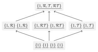
For a finite group , the different SSB phases are nicely organized by the lattice of conjugate subgroups and visualized by a Hasse diagram where the families of conjugate subgroups are connected by the presence of an inclusion map, i.e., when one family is a subgroup of the other. In Fig. S1, we have shown this for the Dihedral symmetries considered in the main text for with the presentation,
| (19) |
A.2 Landau compatibility and incompatibility
We can also distinguish between Landau-compatible and incompatible transitions using the lattice of conjugate subgroups and its Hasse diagram. Two SSB phases represented by two families of conjugate subgroups are Landau-compatible if they are connected in the Hasse diagram by the composition of a sequence of arrows. Physically, we can understand this as follows: If we place ourselves in one of the vacua of the SSB phase with residual symmetries , we can treat it as a standalone system with symmetries . These can be spontaneously broken into a conjugate family of subgroups . All other transitions are Landau incompatible. Physically, a transition between Landau-incompatible phases cannot be understood by a hierarchical splitting of each vacuum, but rather by a more drastic process involving multiple vacua coming together and reorganizing themselves.
In particular the fully symmetric phase with unique vacuum and fully broken phase with vacua are Landau compatible with all SSB phases. The interesting cases are the phases with partial symmetry breaking as we saw in the main text. Landau-compatible transitions are characterized by a change in the number of vacua (although this change does not guarantee compatibility). Moreover, Landau-incompatible transitions can occur between two SSB phases with the same number of vacua, as seen in the main text.
Appendix B More details of the phase diagrams
In this section, we provide more details on the phase diagrams for the classical Hamiltonians considered in the main text:
| (20) |
The important symmetries form the group with the presentation in Eq. 19 and the following action on the planar rotors:
| (21) |
The phase diagrams of Eq. 20 are produced by replacing Eqs. 20 and 17 with the effective continuum gaussian theory in either of the two dual forms
| (22) |
and tracking the scaling dimensions of operators and . Setting , these can be determined directly from Eq. 22 to be
| (23) |
However, for non-zero, these cannot be determined exactly. Nevertheless, when the theory flows to a gaussian theory, the following relation satisfied by Eq. 23 and stated in the main text holds
| (24) |
In this case, we can parametrize the theory using a single parameter which we take to be the scaling dimension of , that determines all other scaling dimensions as well as correlation functions
| (25) |
is a function of all parameters and .
The various phases present in the model are:
-
1.
A trivial paramagnet driven by .
-
2.
Partial symmetry-breaking regions (p-SSB±) driven by for and with vacua
(26) -
3.
Full-Symmetry Breaking Phase (f-SSB) driven by for with vacua
(27) -
4.
A gapless phase when all operators and are irrelevant.
Along the line, it is also useful to define the following critical temperatures:
-
•
, when is marginal, i.e., ,
-
•
when is marginal, i.e., and
-
•
when is marginal, i.e., .
We may ask if there are other perturbations missed in the models we have considered that can qualitatively change the phase diagram. It is easy to verify that there are no other primaries [19] that are allowed by symmetry. For example, , which could connect the and p-SSB± regions, is disallowed by the symmetry. But what about descendants [19]? In particular for , for the only relevant symmetry-allowed primary operator in Eq. 22 is . Discounting the symmetry-disallowed operators, we should consider with dimension . This is symmetry-allowed and would be relevant when . However, this operator is a boundary term and would not affect the bulk phase diagram. We do not explore the interesting question of how the presence of descendants can affect boundary phenomena in this work.
The phase diagram of Eq. 20 is also qualitatively reproduced by the quantum analogues with Hamiltonians of the form
| (28) | ||||
for by identifying via Bethe ansatz [45].
B.1 Double frequency sine-Gordon and f-SSB to p-SSB± Ising transition
The transition between the p-SSB± and f-SSB phases, dominated by and respectively, belongs to the Ising universality class. To understand why, let us focus on where for , is irrelevant, while and are relevant. Thus, the action Eq. 22 reduces to
| (29) |
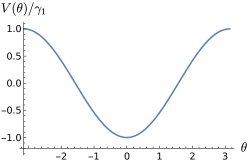
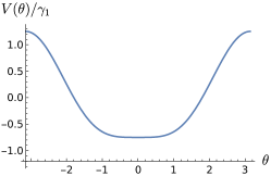
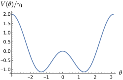
This is the so-called double-frequency Sine-Gordon model [14] whose analysis reveals the Ising transition. Let us understand this by looking at the potential
| (30) |
For , has a unique minimum for large at (for ) and (for ). As we reduce , we see in Fig. S2 that the symmetry is spontaneously broken in the vacuum at . Near this point, we can Taylor expand Eq. 29 to get (after appropriate redefinitions) a 2d real scalar field theory with Ising symmetry
| (31) |
This flows to the Ising universality class at criticality i.e . The same story can be repeated for any by replacing in Eqs. 29 and 30. For large , we will now get minima, but by Taylor expanding around each minimum, we get Eq. 31.
B.2 Self-dual sine-Gordon model and PM to p-SSB± transition
To understand the transition from the symmetry preserving PM and the p-SSB± phases dominated by and respectively, we want to focus on the situation when the two operators have the same scaling dimension. This happens when . We see that the both operators are not irrelevant for when a direct transition can exist. As explained in Ref.[13], this is described by the self-dual Sine-Gordon model
| (32) |
For , when and are both not irrelevant, the fate of Eq. 32 under RG flow was analyzed in Ref. [13]. Their results are summarized as follows:
-
1.
For , Eq. 32 flows to a trivial gapped state. Thus, there is no phase transition between the and dominant regions and they are smoothly connected.
-
2.
For , Eq. 32 flows to the Ising universality class.
-
3.
For , Eq. 32 flows to the 3-state Potts universality class.
- 4.
The RG flow of Eq. 32 is trivial for when and are irrelevant, giving us a gaussian theory. This represents an intermediate gapless phase rather than a direct transition between PM and p-SSB± phases.
B.3 Phase diagrams for
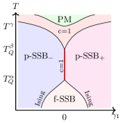
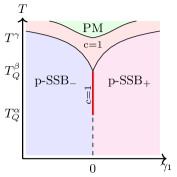
In the main text, we presented phase diagrams for . Here, we discuss the same for . The main difference is in the low-temperature regime. Whereas for we saw the f-SSB phase with all symmetries broken, for we see that the partial symmetry-breaking regions p-SSB± persist but are now separated by a first-order line for where the vacua of both the p-SSB± regions coexist as seen by minimizing . We now combine all this to obtain the phase diagrams for various .
B.4 phase diagrams
Let us begin with the trivial, yet instructive case of the phase diagram for . The only non-trivial symmetry is in Eq. 21 and generates a group.
| (33) |
An interesting observation is the absence of a direct phase transition between the and dominant regions. This was argued from the analysis of the RG flow of the self-dual sine-Gordon model in Eq. 32 with . A much simpler way to see the same fact is to consider the quantum Hamiltonian in Eq. 28
| (34) |
By setting , we get the dominant phase with a product ground state. This is clearly adiabatically connected to the ground state of which is equivalent to the dominated high temperature phase of the classical model.
We see that the nature of the phase diagram depends on the sign of , as discussed before and shown in Fig. S3(a,c). For , the phase diagram is modified as shown in Fig. S3(b). The Ising and first order lines can be analyzed using the double-frequency sine-Gordon potential
| (35) |
and repeating the analysis in Section B.1. The 3-state Potts universality class resulting where the two lines meet at and obtains from the flow of the self-dual sine-Gordon model in Eq. 32 with .
If we further tune (not shown in Fig. S3), we get a continuous unnecessary critical line in the phase diagram for along . This is not stable and needs fine-tuning three parameters, unlike for where the unnecessary criticality needs fine-tuning only one parameter, i.e, .
B.5 phase diagrams
We now consider the model of Eq. 20 whose phase diagrams are shown in Fig. S4. The symmetry group of Eq. 21 is abelian,
| (36) |
The phase diagrams for various values are shown in Fig. S4. We see that a direct Landau-incompatible transition is not stable, and needs fine-tuning two parameters for , i.e., and or . However, this fine-tuning can occur accidentally quite naturally in quantum models with aesthetic appeal. For instance, setting in Eq. 28 yields the XYZ model [3] with a staggered magnetic field,
| (37) |
The phase diagram of Eq. 37 exhibits a direct Landau-incompatible transition. However, this is special to the specific model and unstable to symmetric four-body perturbations introduced by in Eq. 28.
A final interesting feature of Fig. S4 is the presence of symmetry-enriched Ising criticality [15, 16]. Transitions between PM and p-SSB± phases belong to the Ising universality class. However, symmetries act on the two branches in different ways. This is seen from the fact that the order parameters that correspond to the primaries of the Ising CFT transform as different irreducible representations of the symmetry in Eq. 36. It is sufficient to track the primary field . For the transition to p-SSB+, this corresponds to the lattice operator which is charged under but not , while for the transition to p-SSB-, this corresponds to which carries both and charges. The distinct charge assignments mean that the two Ising CFT branches cannot be connected trivially. In Fig. S4, they pass through a different universality class with .
B.6 phase diagrams
The phase diagrams for the Hamiltonian are shown in Fig. S5. The two p-SSB± regions correspond to the same phase and the two branches of transitions between them and the PM belonging to the 3-state Potts universality class are same symmetry-enriched versions. As the unnecessary critical line terminates, the two branches can be connected smoothly.
B.7 phase diagrams
The phase diagram for also presents an interesting case. This is the largest in which there is a direct transition between the PM and p-SSB± phases. This is described by the self-dual sine-Gordon model in Eq. 32 for . The two operators in Eq. 32, i.e., and with the same scaling dimensions are relevant for . For , however, they are marginal and tuning their coefficient induces a flow on the conformal manifold with central charge along the so-called orbifold branch [46]. This branch also describes the critical Ashkin-Teller model [47] and has varying critical exponents, similar to the compact boson branch that describes the direct transition between the p-SSB± phases. It is known that the orbifold and compact boson branches meet at the Kosterlitz-Thouless transition which occurs at [46] for our model.
The two lines of transitions between PM and p-SSB± seem to have different symmetry enrichments seen by tracking the symmetry charges of the order parameters for SSB± and . But, as explained in Ref.[15] and seen in Fig. S6, they are smoothly connected via the KT point without leaving the conformal manifold and should nominally be considered as belonging to the same symmetry-enriched class.
B.8 phase diagrams
Finally, we consider the remaining cases , where a direct transition between the PM and p-SSB± does not exist. Rather there is an intermediate gapless phase. In this region, all symmetry-allowed operators in Eq. 22, i.e., and , are irrelevant. The gapless phase terminates at low temperatures when becomes marginal and at high temperatures when becomes marginal. Along the line, these occur at and respectively. As we increase , the size of the p-SSB± regions shrinks, whereas the gapless phase grows. In the formal limit of , becomes a full symmetry, and we recover the phase diagram of the ordinary classical XY model.
Appendix C Comments on anomalies
The study of anomalous symmetries has a long history in high energy and condensed matter physics in different contexts, which got a fillip with the study of topological phases. Anomalies are non-trivial manifestations of symmetries and are characterized by different properties:
-
1.
They disallow a strictly on-site representation [34].
- 2.
- 3.
These properties are believed to be equivalent, although to the best of our knowledge, this has not been proven yet.
In quantum systems, anomalies can manifest themselves in two distinct ways. The first case is where the microscopic symmetries are anomalous on the full Hilbert space, as in the case of (a) Lieb-Schultz-Mattis (LSM) constrained spin systems [3, 29, 30, 31] where there exists a mixed anomaly between on-site projective representations and lattice symmetries, and (b) boundaries of symmetry protected topological (SPT) phases [48, 7, 49] where symmetries are represented on boundary degrees of freedom as anomalous non-on-site finite depth circuits. These systems do not host a trivial symmetry-preserving phase anywhere in their phase diagrams. The second case is where the microscopic symmetries are not anomalous on the full second-quantized Hilbert space but are anomalous when restricted to certain symmetry sectors. This is the case for LSM constrained fermion systems where a trivial insulator is forbidden at certain fermion densities but not all. By changing the symmetry sector of the ground state, e.g., by tuning a chemical potential or magnetic field, a trivial phase can be obtained in the phase diagram.
In both settings, the anomalies are kinematic and have a clear microscopic origin that can be diagnosed using microscopic probes [30, 50, 51]. Often, it is convenient to employ an effective field-theoretic lens [8, 9, 32] to understand anomalies using gauge fields. This is especially useful in tracking lattice symmetries which often ‘emanate’ to an internal symmetry on the effective low-energy fields [8, 9, 32]. In particular, as shown in Ref [9], anomalies present only under restriction of symmetry sectors manifest themselves in the infrared by acting unfaithfully as a quotient. For instance, spinful fermions on a square lattice with an symmetry, when restricted to half-filling acts as which has an LSM anomaly. These emanant symmetries should be distinguished from emergent ones. The latter are without any microscopic origin and are broken by irrelevant operators, whereas the former are not.