Strongly vs. weakly coupled in-medium showers:
energy stopping in large-$N_{\rm f}$ QED

Abstract

Inside a medium, showers originating from a very high-energy particle may develop via medium-induced splitting processes such as hard bremsstrahlung or pair production. During shower development, two consecutive splittings sometimes overlap quantum mechanically, so that they cannot be treated independently. Some of these effects can be absorbed into an effective value of a medium parameter known as $\hat{q}$. Previous calculations (with certain simplifying assumptions) have found that, after adjusting the value of $\hat{q}$, the leftover effect of overlapping splittings is quite small for purely gluonic large-$N_{\rm c}$ showers but is very much larger for large-$N_{\rm f}$ QED showers, at comparable values of $N\alpha$. Those works did not quite make for apples-to-apples comparisons: the gluon shower work investigated energy deposition from a gluon-initiated shower, whereas the QED work investigated charge-deposition from an electron-initiated shower. As a first step to tighten up the comparison, this paper investigates energy deposition in the QED case. Along the way, we develop a framework that should be useful in the future to explore whether the very small effect of overlapping splitting in purely gluonic showers is an artifact of having ignored quarks.

1 Introduction and Results

1.1 Introduction

When passing through matter, high energy particles lose energy by showering, via the splitting processes of hard bremsstrahlung and pair production. At very high energy, the quantum mechanical duration of each splitting process, known as the formation time, exceeds the mean free time for collisions with the medium, leading to a significant reduction in the splitting rate known as the Landau-Pomeranchuk-Migdal (LPM) effect. The LPM effect was originally worked out for QED in the 1950’s LP1 ; LP2 ; Migdal and then later generalized to QCD in the 1990s by Baier, Dokshitzer, Mueller, Peigne, and Schiff BDMPS1 ; BDMPS2 ; BDMPS3 and by Zakharov Zakharov1 ; Zakharov2 (BDMPS-Z).

Modeling of the development of high-energy in-medium showers typically treats each splitting as an independent dice roll, with probabilities set by calculations of single-splitting rates that take into account the LPM effect. The question then arises whether consecutive splittings in a shower can really be treated as probabilistically independent, or whether there is any significant chance that the formation times of splittings could overlap so that there are significant quantum interference effects entangling one splitting with the next. A number of years ago, several authors Blaizot ; Iancu ; Wu showed, in a leading-log calculation, that the effects of overlapping formation times in QCD showers could become large when one of the two overlapping splittings is parametrically softer than the other. They also showed that those large leading logarithms could be absorbed into a redefinition of the medium parameter $\hat{q}$, which parametrizes the effectiveness with which the medium deflects high-energy particles. A refined question arose: How large are overlapping formation time effects that cannot be absorbed into a redefinition of $\hat{q}$?

To provide a simpler arena than QCD for developing methods and calculational tools to answer this question, ref. qedNfstop first studied it in large-$N_{\rm f}$ QED (where $N_{\rm f}$ is the number of electron flavors). That paper used a thought experiment to determine how important overlap effects could be. Consider a shower initiated by a high-energy electron moving in the $z$ direction, starting at $z=0$. Imagine for simplicity that the medium is static, homogeneous, and of infinite extent. The shower will create more and more electrons, positrons, and photons, of lower and lower energy, eventually depositing various $+$ and $-$ charges into the medium at various positions. Let $\rho(z)$ be the distribution in $z$ of net charge deposited in the medium, statistically averaged over many such showers. Define the charge stopping length $\ell_{\rm stop}^{Q}$ to be the first moment of that distribution, $\ell_{\rm stop}^{Q}\equiv\langle z\rangle_{\rho}\equiv Q^{-1}\int dz\>z\,\rho(z)$, where $Q$ is the charge of the initial electron (and so is the total charge of the shower). Let $\sigma^{Q}$ be the width of the distribution $\rho(z)$. Ignoring overlap effects, both $\ell_{\rm stop}^{Q}$ and $\sigma^{Q}$ scale with $\hat{q}$, coupling constant, and the energy $E_{0}$ of the initial electron as

$$\ell_{\rm stop}\sim\sigma\sim\frac{1}{\alpha}\sqrt{\frac{E_{0}}{\hat{q}}}.$$ (1)

The value of $\hat{q}$ then cancels in the ratio $\sigma/\ell_{\rm stop}$. Any effect that can be absorbed into $\hat{q}$ would not affect the value of $\sigma/\ell_{\rm stop}$, and so that ratio could be used to test how large are overlapping formation time effects that cannot be absorbed into $\hat{q}$. To leading order in $\alpha$, ref. qedNfstop found that the relative size of overlap effects was

$$\mbox{overlap correction}=-87\%\times N_{\rm f}\alpha\qquad\mbox{(large-$N_{\rm f}$ QED charge stopping $\sigma/\ell_{\rm stop}$).}$$ (2)

Later, when we were doing a related calculation finale ; finale2 for large-$N_{\rm c}$ QCD, we fully expected to find an answer of the same order of magnitude, with $N_{\rm c}\alpha_{\rm s}$ playing the role of $N_{\rm f}\alpha$. So far, that calculation has only been completed for purely-gluonic showers. Since gluons have no charge, we studied the energy deposition distribution $\epsilon(z)$ instead of a charge deposition distribution. We similarly define an energy stopping distance $\ell_{\rm stop}^{E}$ and width $\sigma^{E}$, which also scale like (1). We may again look to the ratio $\sigma/\ell_{\rm stop}$ as a vehicle for measuring overlap effects that cannot be absorbed into $\hat{q}$. In the case of QCD, the question of $\hat{q}$ insensitivity of $\sigma/\ell_{\rm stop}$ is quite a bit more subtle than in QED because of enhanced soft emissions in the QCD version of the LPM effect. Those subtleties do not matter for the QED analysis we will carry out in the present paper, and so we will not review them here. (See refs. finale ; finale2 for details.) To our great surprise, the result found for gluon showers was

$$\mbox{overlap correction}=-2\%\times N_{\rm c}\alpha_{\rm s}\qquad\mbox{(large-$N_{\rm c}$ pure-gluon energy stopping $\sigma/\ell_{\rm stop}$).}$$ (3)

For similar values of $N\alpha$, this is a drastically smaller overlap effect than the corresponding QED result (2).

Refs. finale ; finale2 also looked at the shape $S_{\epsilon}(Z)$ of $\epsilon(z)$, defined by $S_{\epsilon}(Z)\equiv\ell_{\rm stop}^{E}\,\epsilon(Z\ell_{\rm stop}^{E})/E_{0}$ where $Z$ represents distance measured in units of $\ell_{\rm stop}$. The width of $S_{\epsilon}(Z)$ is the ratio $\sigma^{E}/\ell_{\rm stop}^{E}$ just discussed. More generally, overlap effects on the full function $S_{\epsilon}(Z)$ were found to be very small for QCD.

There remains the open question of why the QED and QCD results are so very different! Perhaps the tiny result (3) is merely a coincidence, arising from an accidental cancellation for the special case of large-$N_{\rm c}$ purely gluonic showers. Perhaps showers involving fermions behave differently from those that don’t. Or perhaps the shape of energy deposition, in any theory, is for some reason less sensitive to changes (such as from overlap effects) than the shape of charge deposition.

In this paper, we take a first look at the last possibility by calculating the relative size of overlapping formation time effects on the value of $\sigma/\ell_{\rm stop}$ for energy deposition in large-$N_{\rm f}$ QED. An equally important goal is that developing the tools to better analyze overlap effects for the $e^{\pm}$/photon showers will prepare us in later work to add quarks to our QCD showers and so eventually address the other possible explanations as well.

1.2 Results

Our main results for large-$N_{\rm f}$ QED are summarized in table 1. We will discuss later the different choices of renormalization scale shown in the table. That’s a detail that does not impact the qualitative conclusion, which is that the relatively large size of the QED result (2) compared to the gluon shower result (3) is not due to any qualitative difference between charge deposition and energy deposition in the QED case. For large-$N_{\rm f}$ QED, the overlap effects on energy deposition are comparable in size to the ones for charge deposition.

		overlap correction to $\sigma/\ell_{\rm stop}$
deposition distribution	initiating particle	$\mu\propto(\hat{q}E_{0})^{1/4}$	$\mu\propto(\hat{q}E)^{1/4}$	$\begin{matrix}\mu_{e\to e\gamma}\propto(x_{e}\hat{q}E/(1{-}x_{e}))^{1/4}\\ \mu_{\gamma\to e\bar{e}}\propto\bigl{(}x_{e}(1{-}x_{e})\hat{q}E\bigr{)}^{1/4}\end{matrix}$
charge	$e$	$-87\%\times N_{\rm f}\alpha$	$~{}{-}85\%\times N_{\rm f}\alpha$	$~{}{-}80\%\times N_{\rm f}\alpha$
energy	$e$		$+113\%\times N_{\rm f}\alpha$	$+113\%\times N_{\rm f}\alpha$
energy	$\gamma$		$~{}{+}99\%\times N_{\rm f}\alpha$	$~{}{+}98\%\times N_{\rm f}\alpha$

Table 1: The relative size of corrections to the ratio $\sigma/\ell_{\rm stop}$ of width to stopping distance in large-$N_{\rm f}$ QED for the cases of (i) charge deposition of electron-initiated showers, (ii) energy deposition of electron-initiated showers, and (iii) energy deposition of photon-initiated showers. The last three columns correspond to three different prescriptions for the choice of renormalization scale, of which the last two will be used in this paper. The $\mu\propto(\hat{q}E_{0})^{1/4}$ entry for charge deposition of electron-initiated showers is provided merely to make contact with the value (2) of the QED result previously calculated in ref. qedNfstop . The exact proportionality constants in $\mu\propto(\hat{q}E_{0})^{1/4}$ and $\mu\propto(\hat{q}E)^{1/4}$ do not matter; only the energy and $x_{e}$ dependence of $\mu$ affect the results. That’s also true of the specifications of $\mu$ in the last column provided (i) the proportionality constants are chosen the same for $\mu_{e\to e\gamma}$ and $\mu_{\gamma\to e\bar{e}}$ or (ii) one is looking at the charge deposition (which depends only on $\mu_{e\to e\gamma}$ at this order).

1.3 Outline

In the next section, we first discuss the simplifying assumptions made in this paper. We then review diagrams and our notation for (i) LPM/BDMPS-Z in-medium splitting rates [which we call “leading order” rates] and (ii) the corrections to those rates due to overlapping formation times, which we call next-to-leading-order (NLO) corrections. Complicated formulas for the NLO rate corrections may be found in ref. qedNf for large-$N_{\rm f}$ QED, but we will not review those NLO formulas explicitly.

In section 3, we review the concept of net rates $[d\Gamma/dx]_{\rm net}$ used by refs. finale ; finale2 ; qcd (i) to simplify shower evolution equations in cases where there are effective $1{\to}3$ splittings (due to overlap effects) in addition to just $1{\to}2$ splittings and (ii) to provide a convenient way to package numerical results for rates, which can then be fit by analytic functions that are more efficient to evaluate. The previous analysis of refs. finale ; finale2 ; qcd only considered gluons, where all particles are identical, and here we adapt that discussion to the case of distinguishable particles. Some analytic results are also presented, for logarithmic dependence of the net rates when one daughter of an overlapping splitting is soft, with details left to an appendix.

Section 4 discusses sensible choices of ultraviolet (UV) renormalization scale for this problem.

Section 5 reviews the formalism used by ref. qedNfstop to find the earlier overlap correction (2) for $\sigma^{Q}/\ell_{\rm stop}^{Q}$, which is the width of the shape function $S_{\rho}(Z)$ for the charge deposition distribution $\rho(z)$. Results for other moments of the shape are also presented for completeness. Section 6 then generalizes that discussion to the energy deposition distribution $\epsilon(z)$. Both of these sections provide the values presented in table 1.

A very brief conclusion is offered in section 7.

2 Review of the building blocks: splitting rates

2.1 Assumptions

In this paper, we make use of formulas for overlap corrections to splitting rates that were computed for large-$N_{\rm f}$ QED in ref. qedNf and applied to $\sigma/\ell_{\rm stop}$ for charge deposition in ref. qedNfstop . We make the same simplifying assumptions as those papers, similar to those later made in the gluon shower analysis of refs. qcd ; finale ; finale2 . For the splitting rate calculations, we assume a static, homogeneous medium that is large enough to contain (i) formation times in the case of splitting rate calculations and (ii) the entire development of the shower for calculation of overlap corrections to $\sigma/\ell_{\rm stop}$. We will ignore the mass (vacuum and medium-induced) of all high-energy particles. We take the multiple-scattering ($\hat{q}$) approximation for transverse momentum transfer from the medium. (This is equivalent to Migdal’s large Coulomb logarithm approximation Migdal in the case of QED.) We will in particular approximate the bare value $\hat{q}_{(0)}$ of $\hat{q}$ as constant, ignoring any logarithmic energy dependence of $\hat{q}_{(0)}$. (Here $\hat{q}_{(0)}$ represents the value from scattering of the high-energy particle with the medium without any high-energy splitting.) We assume that the particle initiating the shower can be approximated as on-shell. Taking the large-$N_{\rm f}$ limit reduced the number of diagrams that had to be computed in ref. qedNf , somewhat simplified the structure of equations for charge deposition in ref. qedNfstop , and will somewhat simplify the structure of equations for energy deposition in this paper. The overlap corrections qedNf to splitting rates have so far only been computed for $p_{\perp}$-integrated rates because integration over ${\bm{p}}_{\perp}$ makes the calculations much simpler. In any case, $p_{\perp}$-integrated rates are all that we need to study features of charge and energy deposition distributions $\rho(z)$ and $\epsilon(z)$ since we will not keep track of the (parametrically small) spread of the deposition in directions transverse to $z$.

Throughout this paper, we formally treat $N_{\rm f}\alpha(\mu)$ as small, where $\alpha(\mu)$ is the coupling associated with high-energy splitting. Like in the QCD discussion of ref. finale , the relevant scale $\mu$ for the running coupling scales with $\hat{q}$ and energy $E$ as roughly $(\hat{q}E)^{1/4}$. [We’ll discuss detailed choices of $\mu$ later.] Unlike QCD, the running coupling in QED gets larger with increasing energy. That means that, in the QED case, the value of $N_{\rm f}\alpha$ at medium scales would necessarily be small as well. We will not take advantage of that; we summarize all medium effects by the value of $\hat{q}$ in order to (i) simplify the calculation and (ii) make everything as closely parallel to the QCD calculations of refs. finale ; finale2 ; qcd as possible.

2.2 Diagrams

In the $\hat{q}$ approximation, the LPM splitting rates for bremsstrahlung and pair production are

$$\left[\frac{d\Gamma}{dx_{e}}\right]^{\rm LO}_{e\to e\gamma} =\frac{\alpha}{2\pi}\,P_{e\to e}(x_{e})\sqrt{\frac{\hat{q}}{E}\left|\frac{1}{x_{e}}-1\right|},$$ (4a)

$$\left[\frac{d\Gamma}{dx_{e}}\right]^{\rm LO}_{\gamma\to e\bar{e}} =\frac{N_{\rm f}\alpha}{2\pi}\,P_{\gamma\to e}(x_{e})\sqrt{\frac{\hat{q}}{E}\left|\frac{1}{x_{e}}+\frac{1}{1{-}x_{e}}\right|}.$$ (4b)

in the high energy limit. Above, $E$ is the energy of the parent, $x_{e}$ is the energy fraction of the electron daughter, and the $P(x)$ are unregulated Dokshitzer-Gribov-Lipatov-Alterelli-Parisi splitting functions

$$P_{e\to e}(x)=\frac{1+x^{2}}{1-x},\qquad P_{\gamma\to e}(x)=x^{2}+(1{-}x)^{2}.$$ (5)

We refer to (4) as the “leading-order” (LO) rates. For us, leading order means leading order in the number of high-energy splitting vertices and includes the effects of an arbitrary number of interactions with the medium. Adopting Zakharov’s picture Zakharov1 ; Zakharov2 , we think of the rate for $e{\to}e\gamma$ and $\gamma{\to}e\bar{e}$ as time-ordered interference diagrams, such as fig. 1, which combine the amplitude for the splitting (blue) with the conjugate amplitude (red). See refs. 2brem ; qedNf for more discussion of our graphical conventions and implementation of Zakharov’s approach.

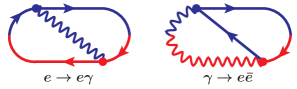
Figure 1: Time-ordered interference diagrams contributing to the rate of $e\to e\gamma$ and $\gamma\to e\bar{e}$. Time runs from left to right. In both cases, all lines implicitly interact with the medium. We need not follow particles after the emission has occurred in both the amplitude and conjugate amplitude because we only calculate the $p_{\perp}$-integrated rate. (See, for example, section 4.1 of ref. 2brem for a more explicit argument, although applied there to more complicated diagrams.) Nor need we follow them before the first emission because we approximate the initial particle as on-shell. Only one of the two time orderings that contribute to each process are shown above but both orderings can be included by taking $2\operatorname{Re}[\cdots]$. (Graphically, complex conjugation corresponds to flipping the diagram around a horizontal axis, exchanging the colors red and blue, and reversing the arrows on the fermion lines.)

There is a factor of $N_{\rm f}$ in the pair production rate (4b) because the produced pair can have any flavor. So, in the large-$N_{\rm f}$ limit, pair production (4b) is parametrically faster than bremsstrahlung (4a). Correspondingly, the overlap of $e\to e\gamma$ with another splitting process is dominated by the overlap $e\to e\gamma\to ee\bar{e}$ (as opposed to $e\to e\gamma\to e\gamma\gamma$ or $\gamma\to e\bar{e}\to e\bar{e}\gamma$). Figs. 2 and 3 show all of time-ordered interference diagrams contributing to the overlap of $e\to e\gamma\to ee\bar{e}$ in the large-$N_{\rm f}$ limit. We refer to these overlap effects as one type of next-to-leading-order (NLO) effect because these diagrams are suppressed by one power of high-energy $N_{\rm f}\alpha(\mu)$ compared to the leading-order process $e\to e\gamma$. The subtraction in fig. 2 means that our rates represent the difference between (i) a full calculation of (potentially overlapping) $e\to e\gamma\to ee\bar{e}$ and (ii) approximating that double splitting as two independent, consecutive single splittings $e{\to}e\gamma$ and $\gamma\to e\bar{e}$ that each occur with the LO single splitting rates (4).

Figure 2: Time-ordered interference diagrams for $e\to ee\bar{e}$ in large-$N_{\rm f}$ QED qedNf . Here, only diagrams with transverse-polarized photons are shown. Complex conjugates of the above interference diagrams should also be included by taking $2\operatorname{Re}[\cdots]$ of the above.

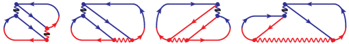
Figure 3: More time-ordered interference diagrams for $e\to ee\bar{e}$ in large-$N_{\rm f}$ QED qedNf . These involve exchange of a longitudinally-polarized photon in light-cone gauge, represented by an instantaneous (in light-cone time) vertical photon line crossed by a bar.

Corresponding virtual corrections to single splitting $e\to e\gamma$, such as the interference between $e\to e\gamma\to ee\bar{e}\to e\gamma$ and LO $e\to e\gamma$, must also be accounted for. Fig. 4 shows the relevant time-ordered interference diagrams.

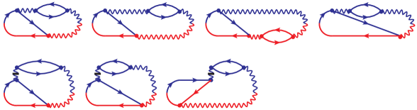
Figure 4: Time-ordered interference diagrams for the virtual correction to $e\to e\gamma$ in large-$N_{\rm f}$ QED qedNf . Again, complex conjugates of these diagrams should be included by taking $2\operatorname{Re}[\cdots]$.

Finally, in the large-$N_{\rm f}$ limit, the only overlap corrections to photon-initiated splitting $\gamma\to e\bar{e}$ are the virtual corrections shown in fig. 5.

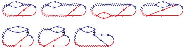
Figure 5: Time-ordered interference diagrams for the virtual correction to $\gamma\to e\bar{e}$ in large-$N_{\rm f}$ QED qedNf .

2.3 Notation for Rates

Consider overlapping bremsstrahlung followed by pair production, $e\to e\gamma\to ee\bar{e}$, whose amplitude is depicted in fig. 6. Here, the pair-produced electrons could have any flavor. It will simplify the rest of our discussion to note that, in the $N_{\rm f}\to\infty$ limit, the two “electron” daughters in the final state become distinguishable: The probability that the flavor of the pair-produced electron is the same as that of the initial electron scales like $1/N_{\rm f}$, and so what we have been calling $e\to e\gamma\to ee\bar{e}$ is actually more akin to $e\to e\gamma\to e\mu\bar{\mu}$. For now, we will emphasize this distinguishability within an overlapping double-splitting process by using the symbol ${\rm E}$ for pair-produced electrons and so will write

$$e\to e\gamma\to e{\rm E}{\bar{\rm E}}.$$ (6)

We will also write LO pair production as $\gamma\to{\rm E}{\bar{\rm E}}$ and the corresponding one-loop virtual correction (the amplitude or conjugate amplitude that has the loop in fig. 5) as

$$\gamma\to{\rm E}^{\prime}{\bar{\rm E}}^{\prime}\to\gamma\to{\rm E}{\bar{\rm E}}.$$ (7)

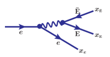
Figure 6: Our notation (6) for distinguishing pair-produced electrons from the original electron in $e\to e\gamma\to ee\bar{e}$ in the large-$N_{\rm f}$ limit. The $x$’s are the energy fractions of the original electron, and $x_{\scriptscriptstyle{{\bar{\rm E}}}}=1-x_{e}-x_{\scriptscriptstyle{{\rm E}}}$.

The basic rates that we will need from ref. qedNf as our initial building blocks are leading-order splitting rates, their NLO corrections, and the overlap correction to $e\to e\gamma\to e{\rm E}{\bar{\rm E}}$. In this paper, we will refer to them as

$$1{\to}2 \left[\frac{d\Gamma}{dx_{e}}\right]_{e\to e\gamma}=\left[\frac{d\Gamma}{dx_{e}}\right]^{\rm LO}_{e\to e\gamma}+\left[\Delta\frac{d\Gamma}{dx_{e}}\right]_{e\to e\gamma}^{\rm NLO},$$ rates: (8a)

$$\left[\frac{d\Gamma}{dx_{\scriptscriptstyle{{\rm E}}}}\right]_{\gamma\to{\rm E}{\bar{\rm E}}}=\left[\frac{d\Gamma}{dx_{\scriptscriptstyle{{\rm E}}}}\right]^{\rm LO}_{\gamma\to{\rm E}{\bar{\rm E}}}+\left[\Delta\frac{d\Gamma}{dx_{\scriptscriptstyle{{\rm E}}}}\right]_{\gamma\to{\rm E}{\bar{\rm E}}}^{\rm NLO},$$ (8b)

effective $$1{\to}3 \left[\Delta\frac{d\Gamma}{dx_{e}\,dx_{\scriptscriptstyle{{\rm E}}}}\right]_{e\to e{\rm E}{\bar{\rm E}}}.$$ rate: (8c)

The symbol $\Delta$ in $[\Delta d\Gamma/dx_{e}\,dx_{\scriptscriptstyle{{\rm E}}}]_{e\to e{\rm E}{\bar{\rm E}}}$ is a reminder that this rate represents a correction (as in fig. 2) to a calculation of double splitting as two, consecutive, independent LO splittings. Explicit formulas for the rates (8) may be found in ref. qedNf , which carried out the calculations using Light Cone Perturbation Theory (LCPT). As discussed in refs. seq ; finale ; finale2 in the context of gluon showers, overlap effects of two consecutive splittings can be accounted for by classical probability analysis of a shower that develops with these $1{\to}2$ splittings and $1{\to}3$ splittings.

3 Net rates: definitions, numerics, and fits

3.1 Basic net rates

In refs. finale ; finale2 , we showed how the NLO evolution of gluon showers could be expressed in terms of the “net” rate $[d\Gamma/dx]_{\rm net}$ for a splitting or pair of overlapping splittings to produce one daughter of energy $xE$ (plus any other daughters) from a parent of energy $E$. We then numerically evaluated the net rate $[d\Gamma/dx]_{\rm net}$ for a mesh of $x$ values and then interpolated using relatively simple fitting functions, which are then used for calculations of shower development. We will use the same strategy here, except that now we have different types of particles ($\gamma$, $e$, and $\bar{e}$) and so need multiple net rates depending on the type of parent and daughter.

In the gluon case, one must be careful about final state, identical particle combinatoric factors when defining the net rate. We may avoid that here, and so simplify the discussion, by using the large-$N_{\rm f}$ distinguishability between a pair-produced electron and the direct heir of the original electron in $e\to e\gamma\to e{\rm E}{\bar{\rm E}}$. Then every daughter in the process $e\to e{\rm E}{\bar{\rm E}}$ is distinguishable, and the same is true of the other NLO or LO processes relevant in the large-$N_{\rm f}$ limit: $e\to e\gamma$ and $\gamma\to{\rm E}{\bar{\rm E}}$.

We now establish notation by listing the basic net rates that we need:

$$\left[\frac{d\Gamma}{dx}\right]^{\rm net}_{{\underline{e\to e}}}=\left[\frac{d\Gamma}{dx}\right]^{\rm LO}_{{\underline{e\to e}}}+\left[\frac{d\Gamma}{dx}\right]^{\rm NLO}_{{\underline{e\to e}}},$$ (9a)

$$\left[\frac{d\Gamma}{dx}\right]^{\rm net}_{{\underline{e\to{\rm E}}}}=\left[\frac{d\Gamma}{dx}\right]^{\rm NLO}_{{\underline{e\to{\rm E}}}},$$ (9b)

$$\left[\frac{d\Gamma}{dx}\right]^{\rm net}_{{\underline{e\to{\bar{\rm E}}}}}=\left[\frac{d\Gamma}{dx}\right]^{\rm NLO}_{{\underline{e\to{\bar{\rm E}}}}},$$ (9c)

$$\left[\frac{d\Gamma}{dx}\right]^{\rm net}_{{\underline{e\to\gamma}}}=\left[\frac{d\Gamma}{dx}\right]^{\rm LO}_{{\underline{e\to\gamma}}}+\left[\frac{d\Gamma}{dx}\right]^{\rm NLO}_{{\underline{e\to\gamma}}},$$ (9d)

$$\left[\frac{d\Gamma}{dx}\right]^{\rm net}_{{\underline{\gamma\to{\bar{\rm E}}}}}=\left[\frac{d\Gamma}{dx}\right]^{\rm net}_{{\underline{\gamma\to{\rm E}}}}=\left[\frac{d\Gamma}{dx}\right]^{\rm LO}_{{\underline{\gamma\to{\rm E}}}}+\left[\frac{d\Gamma}{dx}\right]^{\rm NLO}_{{\underline{\gamma\to{\rm E}}}}.$$ (9e)

Above, underlining of subscripts like ${\underline{e\to e}}$ indicate that we are using the large-$N_{\rm f}$ limit to distinguish pair-produced electrons $({\rm E})$ from other electron daughters ($e$) in overlapping splitting rates. [This notational convention will help us differentiate basic net rates (9) from combined quantities that we will introduce later.] The LO rates in (9) are given by (4) as

$$\left[\frac{d\Gamma}{dx}\right]^{\rm LO}_{{\underline{e\to e}}}\equiv \left[\frac{d\Gamma}{dx_{e}}\right]^{\rm LO}_{e\to e\gamma} x_{e}=x$$ with , (10a)

$$\left[\frac{d\Gamma}{dx}\right]^{\rm LO}_{{\underline{e\to\gamma}}}\equiv \left[\frac{d\Gamma}{dx_{e}}\right]^{\rm LO}_{e\to e\gamma} x_{e}=1-x$$ with , (10b)

$$\left[\frac{d\Gamma}{dx}\right]^{\rm LO}_{{\underline{\gamma\to{\rm E}}}}\equiv \left[\frac{d\Gamma}{dx_{\scriptscriptstyle{{\rm E}}}}\right]^{\rm LO}_{\gamma\to{\rm E}{\bar{\rm E}}} x_{\scriptscriptstyle{{\rm E}}}=x$$ with . (10c)

The ${\underline{e\to{\rm E}}}$ and ${\underline{e\to{\bar{\rm E}}}}$ net rates do not have any leading-order (LO) contribution, since they only arise from the overlapping (and therefore NLO) splitting $e\to e\gamma\to e{\rm E}{\bar{\rm E}}$. The $\gamma{\to}{\rm E}$ and $\gamma{\to}{\bar{\rm E}}$ net rates are equal by charge conjugation. In terms of the building blocks (8) whose formulas are given in ref. qedNf , the NLO net rates in (9) are

$$\left[\frac{d\Gamma}{dx}\right]^{\rm NLO}_{{\underline{e\to e}}} \equiv\left[\Delta\frac{d\Gamma}{dx_{e}}\right]_{e\to e\gamma}^{\rm NLO}+\int_{0}^{1-x_{e}}dx_{\scriptscriptstyle{{\rm E}}}\>\left[\Delta\frac{d\Gamma}{dx_{e}\,dx_{\scriptscriptstyle{{\rm E}}}}\right]_{e\to e{\rm E}{\bar{\rm E}}} x_{e}=x$$ with , (11a)

$$\left[\frac{d\Gamma}{dx}\right]^{\rm NLO}_{{\underline{e\to{\rm E}}}} \equiv\int_{0}^{1-x_{\scriptscriptstyle{{\rm E}}}}dx_{e}\>\left[\Delta\frac{d\Gamma}{dx_{e}\,dx_{\scriptscriptstyle{{\rm E}}}}\right]_{e\to e{\rm E}{\bar{\rm E}}} x_{\scriptscriptstyle{{\rm E}}}=x$$ with , (11b)

$$\left[\frac{d\Gamma}{dx}\right]^{\rm NLO}_{{\underline{e\to{\bar{\rm E}}}}} \equiv\int_{0}^{1-x_{\scriptscriptstyle{{\bar{\rm E}}}}}dx_{e}\>\biggl{(}\left[\Delta\frac{d\Gamma}{dx_{e}\,dx_{\scriptscriptstyle{{\rm E}}}}\right]_{e\to e{\rm E}{\bar{\rm E}}}\biggr{)}_{\!\!x_{\scriptscriptstyle{{\rm E}}}=1-x_{e}-x_{\scriptscriptstyle{{\bar{\rm E}}}}} x_{\scriptscriptstyle{{\bar{\rm E}}}}=x$$ with (11c)

$$\left[\frac{d\Gamma}{dx}\right]^{\rm NLO}_{{\underline{e\to\gamma}}} \equiv\left[\Delta\frac{d\Gamma}{dx_{e}}\right]_{e\to e\gamma}^{\rm NLO} x_{e}=1-x$$ with , (11d)

$$\left[\frac{d\Gamma}{dx}\right]^{\rm NLO}_{{\underline{\gamma\to{\rm E}}}} \equiv\left[\Delta\frac{d\Gamma}{dx_{\scriptscriptstyle{{\rm E}}}}\right]_{\gamma\to{\rm E}{\bar{\rm E}}}^{\rm NLO} x_{\scriptscriptstyle{{\rm E}}}=x$$ with . (11e)

Because all the daughters of our splitting processes $e{\to}e\gamma$, $e{\to}e{\rm E}{\bar{\rm E}}$, and $\gamma{\to}{\rm E}{\bar{\rm E}}$ are distinguishable in large-$N_{\rm f}$, the total rates for splitting of electrons or photons are given in terms of net rates by simply

$$\Gamma_{e} =\int_{0}^{1}dx\>\left[\frac{d\Gamma}{dx}\right]^{\rm net}_{\underline{e\to e}},$$ (12a)

$$\Gamma_{\gamma} =\int_{0}^{1}dx\>\left[\frac{d\Gamma}{dx}\right]^{\rm net}_{\underline{\gamma\to{\rm E}}}=\int_{0}^{1}dx\>\left[\frac{d\Gamma}{dx}\right]^{\rm net}_{\underline{\gamma\to{\bar{\rm E}}}},$$ (12b)

without any identical-particle final state factors such as those appearing in the analysis of $g{\to}gg$ and $g{\to}ggg$ in refs. finale ; finale2 . Regarding (12a), note that $[d\Gamma/dx]_{\underline{e\to e}}$ accounts for both of the processes $e\to e{\rm E}{\bar{\rm E}}$ and $e\to e\gamma$ that contribute to the effective electron splitting rate, whereas, for example, integrating $[d\Gamma/dx]_{\underline{e\to{\rm E}}}$ or $[d\Gamma/dx]_{\underline{e\to{\bar{\rm E}}}}$ would account only for $e\to e{\rm E}{\bar{\rm E}}$.

3.2 Numerics and Fits

3.2.1 Basic net rates

Using the formulas from ref. qedNf for the basic rates (9), numerical integration gives results for the NLO contributions (11) to the net rates $[d\Gamma/dx]^{\rm net}_{\underline{i\to j}}$ as functions of $x$. Those numerical integrations are sufficiently time consuming that, following ref. finale2 , we will want to find a way to accurately approximate the numerical results by relatively simple analytic functions of $x$, which can then be used for numerically efficient calculations of shower development.

In order to fit numerical results for the $[d\Gamma/dx]^{\rm net}_{\underline{i\to j}}$ to analytic forms, it is convenient to first transform the $[d\Gamma/dx]^{\rm net}_{\underline{i\to j}}$ into smoother functions by factoring out as much as we can determine about their singular behavior as $x\to 0$ and $x\to 1$. In ref. finale2 , which analyzed overlap effects for purely gluonic showers in QCD, the NLO net rate for $g\to g$ had the same power-law behavior as the leading-order rate, and so it was easier to search for a good analytic fit to the NLO/LO ratio $[d\Gamma/dx]^{\rm NLO}_{g\to g}/[d\Gamma/dx]^{\rm LO}_{g\to g}$ than to find a good fit directly to $[d\Gamma/dx]^{\rm NLO}_{g\to g}$. In the study here of large-$N_{\rm f}$ QED, we modify that procedure because the power-law divergences of the NLO net rate as $x\to 0$ or $1$ do not always match that of the corresponding leading-order rate.

We will define the smoother functions $f_{\underline{i\to j}}(x)$ in terms of ratios $\left[\frac{d\Gamma}{dx}\right]^{\rm NLO}_{\underline{i\to j}}/R_{\underline{i\to j}}(x)$ where the $R(x)$’s are chosen to be simple functions with the same power-law divergences as the NLO net rates. Specifically, we take

$$R_{\underline{e\to e}}(x_{e}) \equiv x_{e}^{-1/2}(1{-}x_{e})^{-3/2}\,\frac{N_{\rm f}\alpha^{2}}{2\pi}\sqrt{\frac{\hat{q}}{E}}\,,$$ (13a)

$$R_{\underline{e\to{\rm E}}}(x_{\scriptscriptstyle{{\rm E}}}) \equiv x_{\scriptscriptstyle{{\rm E}}}^{-3/2}(1{-}x_{\scriptscriptstyle{{\rm E}}})^{+1/2}\,\frac{N_{\rm f}\alpha^{2}}{2\pi}\sqrt{\frac{\hat{q}}{E}}\,,$$ (13b)

$$R_{\underline{e\to\gamma}}(x_{\gamma}) \equiv R_{\underline{e\to e}}(1{-}x_{\gamma}),$$ (13c)

$$R_{\underline{\gamma\to{\rm E}}}(x_{\scriptscriptstyle{{\rm E}}}) \equiv x_{\scriptscriptstyle{{\rm E}}}^{-1/2}(1{-}x_{\scriptscriptstyle{{\rm E}}})^{-1/2}\,\frac{N_{\rm f}^{2}\alpha^{2}}{2\pi}\sqrt{\frac{\hat{q}}{E}}\,.$$ (13d)

[Above, we’ve written the arguments $x$ of $R(x)$ as explicitly $x_{e}$, $x_{\scriptscriptstyle{{\rm E}}}$, etc. as a reminder of exactly what the argument refers to for each type of net rate.] We emphasize that there is nothing fundamental about these exact choices of the $R(x)$’s; they are merely the particular choices we made to simplify finding good fits.

We also found it convenient to isolate certain logarithms, associated with the $\overline{\mbox{MS}}$ renormalization scale $\mu$. Those logarithms appear in rates that include loop corrections. Specifically, we now define our “smooth” functions $f_{\underline{i\to j}}$ in terms of the numerically-computed NLO rates $[d\Gamma/dx]^{\rm NLO}_{\underline{i\to j}}$ by

$$\left[\frac{d\Gamma}{dx}\right]^{\rm NLO}_{\underline{i\to j}}=L_{\underline{i\to j}}(x,\mu)+f_{\underline{i\to j}}(x)\,R_{\underline{i\to j}}(x),$$ (14)

where

$$L_{\underline{e\to e}}(x_{e},\mu)\equiv-\frac{\beta_{0}\alpha}{2}\left[\frac{d\Gamma}{dx_{e}}\right]_{\rm LO}^{e\to e\gamma}\ln\left(\frac{\mu^{2}}{\sqrt{\frac{(1{-}x_{e})\hat{q}E}{x_{e}}}}\right),$$ (15a)

$$L_{\underline{e\to{\rm E}}}\equiv L_{\underline{e\to{\bar{\rm E}}}}\equiv 0,$$ (15b)

$$L_{\underline{e\to\gamma}}(x_{\gamma},\mu)\equiv L_{\underline{e\to e}}(1{-}x_{\gamma},\mu),$$ (15c)

$$L_{\underline{\gamma\to{\rm E}}}(x_{\scriptscriptstyle{{\rm E}}},\mu)\equiv-\frac{\beta_{0}\alpha}{2}\left[\frac{d\Gamma}{dx_{\scriptscriptstyle{{\rm E}}}}\right]_{\rm LO}^{\gamma\to{\rm E}{\bar{\rm E}}}\ln\left(\frac{\mu^{2}}{\sqrt{\hat{q}E}}\right),$$ (15d)

and where

$$\beta_{0}=\frac{2N_{\rm f}}{3\pi}$$ (16)

is the coefficient of the 1-loop renormalization group $\beta$-function for $\alpha$. As will be seen shortly, the $L$’s above do not capture all of the logarithmic dependence of the net rates on $x$ and $1{-}x$. Our particular choice of $x$ dependence (or lack of it) inside the logarithms of (15a) and (15d) is just a matter of convention for our definition (14) of $f_{\underline{i\to j}}(x)$. Readers need not ponder the logic of that choice too deeply; mostly it is a combination of guesses we made early in our work combined with some convenient choices for finding fits.

With these definitions, table 2 and the data points in fig. 7 present our numerical results for the functions $f_{\underline{i\to j}}(x)$. The corresponding numerical results for our net rates (9) can be reconstructed using (14). There is only a single, joint column for $f_{\underline{e\to{\rm E}}}$ and $f_{\underline{e\to{\bar{\rm E}}}}$ in the table because they turn out to be equal:

$$\left[\frac{d\Gamma}{dx}\right]^{\rm NLO}_{{\underline{e\to{\rm E}}}}=\left[\frac{d\Gamma}{dx}\right]^{\rm NLO}_{{\underline{e\to{\bar{\rm E}}}}}$$ (17)

(where, like everywhere in this paper, the large-$N_{\rm f}$ limit is implicit). We are not currently aware of any symmetry argument or other high-level explanation for this equality. Instead, we discovered numerically that the differential rate $[\Delta\,d\Gamma/dx_{e}\,dx_{\scriptscriptstyle{{\rm E}}}]_{e\to e{\rm E}{\bar{\rm E}}}$ appearing in (11) is symmetric under $x_{\scriptscriptstyle{{\rm E}}}\to 1{-}x_{e}{-}x_{\scriptscriptstyle{{\rm E}}}$ (i.e. $x_{\scriptscriptstyle{{\rm E}}}\leftrightarrow x_{\scriptscriptstyle{{\bar{\rm E}}}}$). See appendix A for some (low-level) insight into why the formula qedNf for $[\Delta\,d\Gamma/dx_{e}\,dx_{\scriptscriptstyle{{\rm E}}}]_{e\to e{\rm E}{\bar{\rm E}}}$ has this property.

$x$	$f_{\underline{e\to e}}$	$\begin{array}[]{c}f_{\underline{e\to{\rm E}}}\\ f_{\underline{e\to{\bar{\rm E}}}}\end{array}$	$f_{\underline{e\to\gamma}}$	$f_{\underline{\gamma\to{\rm E}}}$
0.0001	-0.1786	4.7199	-0.5889	-0.0099
0.0005	-0.1777	3.9637	-0.5890	-0.0063
0.001	-0.1774	3.6357	-0.5886	-0.0037
0.005	-0.1745	2.8618	-0.5865	0.0066
0.01	-0.1712	2.5200	-0.5839	0.0135
0.025	-0.1620	2.0564	-0.5763	0.0250
0.05	-0.1472	1.6960	-0.5635	0.0350
0.075	-0.1324	1.4820	-0.5509	0.0411
0.1	-0.1173	1.3296	-0.5384	0.0451
0.15	-0.0856	1.1158	-0.5138	0.0500
0.2	-0.0508	0.9665	-0.4899	0.0526
0.25	-0.0118	0.8535	-0.4666	0.0540
0.3	0.0323	0.7638	-0.4440	0.0547
0.35	0.0828	0.6908	-0.4220	0.0550
0.4	0.1410	0.6306	-0.4009	0.0551
0.45	0.2085	0.5805	-0.3805	0.0552
0.5	0.2871	0.5390	-0.3608	0.0552
0.55	0.3792	0.5054	-0.3420	0.0552
0.6	0.4877	0.4789	-0.3241	0.0551
0.65	0.6166	0.4593	-0.3070	0.0550
0.7	0.7711	0.4467	-0.2910	0.0547
0.75	0.9590	0.4410	-0.2762	0.0540
0.8	1.1927	0.4427	-0.2629	0.0526
0.85	1.4937	0.4519	-0.2517	0.0500
0.9	1.9083	0.4692	-0.2441	0.0451
0.925	2.1920	0.4810	-0.2431	0.0411
0.95	2.5759	0.4951	-0.2461	0.0350
0.975	3.1929	0.5114	-0.2598	0.0250
0.99	3.9530	0.5223	-0.2888	0.0135
0.995	4.5022	0.5261	-0.3160	0.0066
0.999	5.7373	0.5293	-0.3889	-0.0037
0.9995	6.2612	0.5297	-0.4228	-0.0063
0.9999	7.4724	0.5299	-0.5051	-0.0099

Table 2: Results for the functions $f_{\underline{i\to j}}(x)$ extracted from numerical computation of the net rates (9) using the explicit formulas of ref. qedNf . Numerical results for the rates were translated into numerical results for $f_{\underline{i\to j}}$ using the definition (14) of the $f_{\underline{i\to j}}$. The results for $f_{\underline{e\to{\rm E}}}$ and $f_{\underline{e\to{\bar{\rm E}}}}$ are equal to each other.

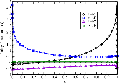
Figure 7: Plots of numerically-computed data points (table 2) and fits (18) for the functions $f_{\underline{i\to j}}(x)$ defined by (14).

We have found the following, reasonably good fits to the numerical rates and will use these fits for all subsequent calculations in this paper:

$$f_{\underline{e\to e}}(x)=-\tfrac{3}{4}\ln(1{-}x)-22.65461+43.86814\,x-20.48818\,x^{2}+5.29318\,x^{3}\\ +0.01427\,x^{1/2}-1.18685\,x^{3/2}-4.27886\,x^{5/2}\\ -0.16141\,(1{-}x)^{1/2}+12.59425\,(1{-}x)^{3/2}+10.04309\,(1{-}x)^{5/2},$$ (18a)

$$f_{\underline{e\to{\rm E}}}(x)=f_{\underline{e\to{\bar{\rm E}}}}(x)=-\tfrac{22}{15\pi}\ln x+10.45176-25.05713\,x+0.71056\,x^{2}-6.76246\,x^{3}\\ -0.40871\,x^{1/2}+8.94044\,x^{3/2}+12.65584\,x^{5/2}\\ -0.02067\,(1{-}x)^{1/2}-2.06985\,(1{-}x)^{3/2}-7.93648\,(1{-}x)^{5/2},$$ (18b)

$$f_{\underline{e\to\gamma}}(x)=\tfrac{1}{6\pi}\ln(1{-}x)-4.13754+8.91233\,x-4.00731\,x^{2}+1.69990\,x^{3}\\ -0.00903\,x^{1/2}-0.56996\,x^{3/2}-1.90189\,x^{5/2}\\ -0.27947\,(1{-}x)^{1/2}+1.19712\,(1{-}x)^{3/2}+2.63102\,(1{-}x)^{5/2},$$ (18c)

$$f_{\underline{\gamma\to{\rm E}}}(x)=-0.01296+0.31063\,\bigl{(}x(1{-}x)\bigr{)}^{1/2}-0.49837\,x(1{-}x)\\ +0.44890\,\bigl{(}x(1{-}x)\bigr{)}^{3/2}-0.29930\,\bigl{(}x(1{-}x)\bigr{)}^{2}.$$ (18d)

When making fits, the coefficients of logarithms $\ln x$ and $\ln(1{-}x)$ were fixed to the exact values shown above, while all other coefficients were allowed to float to whatever values gave the best fit. Appendix B discusses how (either directly or indirectly) the logarithms can be understood as arising from vacuum-like DGLAP initial (or final) radiation corrections to leading order (BDMPS-Z) single emission processes, and how their coefficients may then be computed analytically.

The fits (18) match every data point of table 2 to better than 0.0008 absolute error.

A convenience of our particular choices of $L_{\underline{e\to e}}(x_{e},\mu)$ and $L_{\underline{\gamma\to{\rm E}}}(x_{\scriptscriptstyle{{\rm E}}},\mu)$ in (15) was the removal of a number of logarithmic terms in the $f_{\underline{i\to j}}$. Our choice of $L_{\underline{\gamma\to{\rm E}}}$ removed the need for $\ln x_{\scriptscriptstyle{{\rm E}}}$ and symmetrically $\ln(1{-}x_{\scriptscriptstyle{{\rm E}}})$ terms in $f_{\underline{\gamma\to{\rm E}}}(x_{\scriptscriptstyle{{\rm E}}})$. (See appendix B for numerical evidence.) Our choice of $L_{\underline{e\to e}}$ did the same for $\ln x_{e}$ in $f_{\underline{e\to e}}(x_{e})$. [However, our choice of $\ln(1{-}x_{e})$ dependence in $L_{e\to e}$ has no bearing on the $\ln(1{-}x_{e})$ term in our fit for $f_{\underline{e\to e}}(x_{e})$ and was chosen for historical reasons.]

3.2.2 Decomposition of $[d\Gamma/dx]^{\rm NLO}_{e\to e}$ into real and virtual parts

The NLO net rate $[d\Gamma/dx]^{\rm NLO}_{\underline{e\to e}}$ gets contributions from both (i) virtual corrections to single splitting $e\to e\gamma$ and (ii) real double splitting $e\to e\gamma\to e{\rm E}{\bar{\rm E}}$, respectively corresponding to the two terms in (11a). Though not necessary for our final numerical results, it will sometimes be insightful to look at these two contributions separately. For that purpose, let’s correspondingly break down $f_{\underline{e\to e}}$ into

$$f_{\underline{e\to e}}(x)=f_{e\to e}^{\rm virt}(x)+f_{e\to e}^{\rm real}(x).$$ (19)

By virtue of (11), these two pieces of $f_{\underline{e\to e}}$ can be reconstructed from the data points in table 2, or from the fits of (18), as

$$f_{e\to e}^{\rm virt}(x)=f_{\underline{e\to\gamma}}(1-x)\quad\mbox{and}\quad f_{e\to e}^{\rm real}(x)=f_{\underline{e\to e}}(x)-f_{\underline{e\to\gamma}}(1-x).$$ (20)

The corresponding contributions to the net rate $[d\Gamma/dx]^{\rm NLO}_{\underline{e\to e}}$ are respectively

$$\left[\Delta\frac{d\Gamma}{dx_{e}}\right]_{e\to e\gamma}^{\rm NLO}=L_{\underline{e\to e}}(x,\mu)+f_{e\to e}^{\rm virt}(x)\,R_{\underline{e\to e}}(x)$$ (21)

and

$$\int_{0}^{1-x_{e}}dx_{\scriptscriptstyle{{\rm E}}}\>\left[\Delta\frac{d\Gamma}{dx_{e}\,dx_{\scriptscriptstyle{{\rm E}}}}\right]_{e\to e{\rm E}{\bar{\rm E}}}=f_{e\to e}^{\rm real}(x)\,R_{\underline{e\to e}}(x).$$ (22)

From (18) and (20), our fits to the real and virtual contributions for $f_{\underline{e\to e}}$ are

$$f_{e\to e}^{\rm real}(x)=-\tfrac{1}{6\pi}\ln x-\tfrac{3}{4}\ln(1{-}x)-25.12199+49.86555\,x-21.58057\,x^{2}+6.99308\,x^{3}\\ +0.29374\,x^{1/2}-2.38397\,x^{3/2}-6.90988\,x^{5/2}\\ -0.15238\,(1{-}x)^{1/2}+13.16421\,(1{-}x)^{3/2}+11.94498\,(1{-}x)^{5/2},$$ (23a)

$$f_{e\to e}^{\rm virt}(x)=\tfrac{1}{6\pi}\ln x+2.46738-5.99741\,x+1.09239\,x^{2}-1.69990\,x^{3}\\ -0.27947\,x^{1/2}+1.19712\,x^{3/2}+2.63102\,x^{5/2}\\ -0.00903\,(1{-}x)^{1/2}-0.56996\,(1{-}x)^{3/2}-1.90189\,(1{-}x)^{5/2}.$$ (23b)

4 Choices of Renormalization Scale $\mu$

4.1 QED versions of earlier scale choices

In the context of purely-gluonic showers in QCD, refs. finale ; finale2 discussed three different choices of an infrared (IR) factorization scale $\Lambda_{\rm fac}$ (introduced to factorize out soft-radiation double logs arising in QCD in the $\hat{q}$ approximation LMW ), which were used to also set scales for the ultraviolet (UV) renormalization scale $\mu$ [as $\mu=(\hat{q}_{\rm A}\Lambda_{\rm fac})^{1/4}$]. A soft-radiation factorization scale $\Lambda_{\rm fac}$ is unnecessary in the QED case since the $\hat{q}$ approximation in QED is not afflicted by soft-radiation double logarithms that appear in QCD. So, we need focus only on $\mu$ in this paper. One way to characterize the choice of $\mu$ made in refs. finale ; finale2 is that it is the scale of the total transverse momentum kick that the medium gives to the high-energy particles during a typical formation time $t_{\rm form}$, which in the $\hat{q}$ approximation is

$$\mu\sim\Delta p_{\perp}\sim\sqrt{\hat{q}t_{\rm form}}\,.$$ (24)

In the BDMPS-Z formalism for single splitting processes, the calculation of splitting rates in the $\hat{q}$ approximation is formally related to a two-dimensional non-relativistic harmonic oscillator quantum mechanics problem with a complex frequency of oscillation given by

$$\mbox{QCD $~{}g{\to}gg$}\,: \qquad\Omega=\sqrt{-\frac{i\hat{q}_{\rm A}}{2E}\left(-1+\frac{1}{x}+\frac{1}{1{-}x}\right)}\,,$$ (25a)

$$\mbox{QED $~{}e{\to}e\gamma$}\,: \qquad\Omega=\sqrt{-\frac{i\hat{q}}{2E}\left(-1+\frac{1}{x_{e}}+0\right)}\,,$$ (25b)

$$\mbox{QED $\gamma{\to}{\rm E}{\bar{\rm E}}$}: \qquad\Omega=\sqrt{-\frac{i\hat{q}}{2E}\left(0+\frac{1}{x_{\scriptscriptstyle{{\rm E}}}}+\frac{1}{1{-}x_{\scriptscriptstyle{{\rm E}}}}\right)}\,.$$ (25c)

The formation time is characterized by the time scale $1/|\Omega|$. Focusing only on parametric behavior, the scale choice (24) would be

$$\mbox{QCD $~{}g{\to}gg$}\,: \qquad\mu\sim\bigl{(}x(1{-}x)\hat{q}E\bigr{)}^{1/4},$$ (26a)

$$\mbox{QED $~{}e{\to}e\gamma$}\,: \qquad\mu\sim\left(\frac{x_{e}\hat{q}E}{x_{\gamma}}\right)^{1/4},$$ (26b)

$$\mbox{QED $\gamma{\to}{\rm E}{\bar{\rm E}}$}: \qquad\mu\sim(x_{\scriptscriptstyle{{\rm E}}}x_{\scriptscriptstyle{{\bar{\rm E}}}}\hat{q}E)^{1/4}.$$ (26c)

In the $g{\to}gg$ case, this was our preferred choice of $\mu$ in refs. finale ; finale2 . The QED version was used for the results in the last column of our table 1.

Refs. finale ; finale2 noted that soft emissions ($x$ or $1{-}x\ll 1$) do not contribute significantly to the shape of energy deposition in the case of an infinite medium, and so one could ignore the $x$ dependence in (26) and instead simply choose $\mu\sim(\hat{q}E)^{1/4}$ as in the next-to-last column of table 1. Refs. finale ; finale2 also noted that splittings with $E\ll E_{0}$, in a shower that started with energy $E_{0}$, do not significantly affect where energy is deposited, and so one could alternatively use the constant value $\mu\sim(\hat{q}E_{0})^{1/4}$ for all the splittings in the shower, as in the third column of table 1.

To summarize for future reference, the three choices of renormalization scale for QED just discussed are

$$\mu \propto(\hat{q}E_{0})^{1/4},$$ (27a)

$$\mu \propto(\hat{q}E)^{1/4},$$ (27b)

$$[\mu_{e\to e\gamma},\mu_{\gamma\to{\rm E}{\bar{\rm E}}}] \propto\bigl{[}(x_{e}\hat{q}E/x_{\gamma})^{1/4}\,,\,(x_{\scriptscriptstyle{{\rm E}}}x_{\scriptscriptstyle{{\bar{\rm E}}}}\hat{q}E)^{1/4}\bigr{]}.$$ (27c)

The choice of overall proportionality constant represented by proportionality signs above will not affect our results for $\sigma/\ell_{\rm stop}$ nor, more generally, any aspect of the shapes $S_{\rho}(Z)$ and $S_{\epsilon}(Z)$ of charge deposition $\rho(z)$ or energy deposition $\epsilon(z)$.

We will use (27) [and especially the last two cases] to test how sensitive our results are to different choices of renormalization scale. One may already see from table 1 that different reasonable choices do not make much of a difference, and so it is not necessary to obsess over which choice is best motivated.

The analogous discussion of refs. finale ; finale2 considered using (24) and retaining the $x$ dependence [as in (27c) here] to be the most physically motivated choice. We now find that assessment somewhat less compelling because there is a different choice of $x$-dependent scale one might consider, which also has a reasonable physical motivation.

4.2 A different choice

Instead of setting the renormalization scale to the transverse momentum scale of (24), one might consider setting $\mu^{2}$ to be of order the combined invariant mass $p^{\mu}p_{\mu}\equiv(p_{2}{+}p_{3})^{\mu}(p_{2}{+}p_{3})_{\mu}$ of the two daughters (labeled here as particles “2” and “3”) of a single BDMPS-Z splitting such as $g{\to}gg$, $e\to e\gamma$ or $\gamma\to{\rm E}{\bar{\rm E}}$. This is equivalent to $\mu^{2}\sim|\vec{p}_{\rm COM}|^{2}$, where $\pm\vec{p}_{\rm COM}$ are the 3-momenta of the daughters in their center-of-momentum frame. We leave the details of the parametric analysis to appendix C, but the result is

$$\mu^{2}\sim(p_{2}{+}p_{3})^{\mu}(p_{2}{+}p_{3})_{\mu}\sim\frac{E}{t_{\rm form}}\,,$$ (28)

which differs from (24) when one of the daughters is soft. In particular, (25) and $t_{\rm form}\sim 1/|\Omega|$ now give

$$\mbox{QCD $~{}g{\to}gg$}\,: \qquad\mu\sim\left(\frac{\hat{q}E}{x(1{-}x)}\right)^{1/4},$$ (29a)

$$\mbox{QED $~{}e{\to}e\gamma$}\,: \qquad\mu\sim\left(\frac{x_{\gamma}\hat{q}E}{x_{e}}\right)^{1/4},$$ (29b)

$$\mbox{QED $\gamma{\to}{\rm E}{\bar{\rm E}}$}: \qquad\mu\sim\left(\frac{\hat{q}E}{x_{\scriptscriptstyle{{\rm E}}}x_{\scriptscriptstyle{{\bar{\rm E}}}}}\right)^{1/4}$$ (29c)

in contrast to (26).

Table 3 shows an expanded version of table 1 in which we have added a column for the new renormalization scale choice (29). The uncertainty about whether the most sensible choice of renormalization scale should be (24) or (28) symmetrically brackets (within round-off error) the $\mu{\propto}(\hat{q}E)^{1/4}$ result. This is because the $x$-dependencies of $\mu$ in (24) and (28) are inverse to each other (while the $\hat{q}$ and $E$ dependence is the same), and so their difference from $\mu\propto(\hat{q}E)^{1/4}$ will generate opposite changes to the logarithms $L_{\underline{i\to j}}$ of (15) and so opposite changes to NLO quantities.

		overlap correction to $\sigma/\ell_{\rm stop}$
	$\mu\propto(\hat{q}E_{0})^{1/4}$	$\begin{matrix}\scriptstyle{\mu_{e\to e\gamma}{\propto}(x_{\gamma}\hat{q}E/x_{e})^{1/4}}\\ \scriptstyle{\mu_{\gamma\to e\bar{e}}{\propto}\bigl{(}\hat{q}E\bigr{/}x_{e}x_{\gamma})^{1/4}}\end{matrix}$	$\mu\propto(\hat{q}E)^{1/4}$	$\begin{matrix}\scriptstyle{\mu_{e\to e\gamma}{\propto}(x_{e}\hat{q}E/x_{\gamma})^{1/4}}\\ \scriptstyle{\mu_{\gamma\to e\bar{e}}{\propto}\bigl{(}x_{e}x_{\gamma}\hat{q}E\bigr{)}^{1/4}}\end{matrix}$
charge, $e$	$-87.0\%\times N_{\rm f}\alpha$	$~{}{-}88.7\%\times N_{\rm f}\alpha$	$~{}{-}84.6\%\times N_{\rm f}\alpha$	$~{}{-}80.4\%\times N_{\rm f}\alpha$
energy, $e$		$+113.6\%\times N_{\rm f}\alpha$	$+113.1\%\times N_{\rm f}\alpha$	$+112.5\%\times N_{\rm f}\alpha$
energy, $\gamma$		$~{}{+}99.4\%\times N_{\rm f}\alpha$	$~{}{+}98.6\%\times N_{\rm f}\alpha$	$~{}{+}97.9\%\times N_{\rm f}\alpha$

Table 3: Like table 1 except that we have inserted a new column (the second column of numbers) for the choice (29) of renormalization scale, and we have included an extra significant digit in our results to make clear that the values in the second and fourth columns of numbers symmetrically bracket those in the third column (within round-off error).

Because of this reflection symmetry about the $\mu{\sim}(\hat{q}E)^{1/4}$ result, we will not bother explicitly showing (28) for results in this paper other than $\ell_{\rm stop}/\sigma$. We will just show results for (27b) and (27c) to give a sense of the variation of results for different reasonable choices of renormalization scale.

5 Charge stopping revisited

For large-$N_{\rm f}$ QED, ref. qedNfstop analyzed the size of overlap corrections to the “$\hat{q}$-independent” ratio $\sigma/\ell_{\rm stop}$ of the width $\sigma$ of the charge-stopping distribution $\rho(z)$ compared to the stopping length $\ell_{\rm stop}\equiv\langle z\rangle_{\rho}$. In this section, we review that analysis in preparation for later discussion of energy deposition in large-$N_{\rm f}$ QED. Here we will update the notation and renormalization scales choices of ref. qedNfstop to be closer to the related analysis of QCD energy deposition in refs. finale ; finale2 , and we will use the fit to the relevant NLO net rate (11a) to greatly simplify numerics.

5.1 Basic equation

Because of the equality (17) of the net rates $[d\Gamma/dx]_{\underline{e\to{\rm E}}}$ and $[d\Gamma/dx]_{\underline{e\to{\bar{\rm E}}}}$, the ${\rm E}$ and ${\bar{\rm E}}$ in $e\to e{\rm E}{\bar{\rm E}}$ will (statistically) be produced with the same distribution in energy, and so they will subsequently deposit charge in exactly the same way (statistically) except for sign, and so their contributions to the total charge deposition $\rho(z)$ will exactly cancel. Only the fate of the $e$ daughter of (large-$N_{\rm f}$) $e\to e{\rm E}{\bar{\rm E}}$ will matter for charge deposition. The only rate we need from (9) is therefore $[d\Gamma/dx]_{\underline{e\to e}}$. (The situation will be more complicated when we later discuss energy deposition.)

Following ref. qedNfstop , our starting equation is

$$\rho(E,z+\Delta z)=[1-\Gamma_{e}(E)\,\Delta z]\,\rho(E,z)+\int_{0}^{1}dx\>\left[\frac{d\Gamma}{dx}(E,x)\right]^{\rm net}_{\underline{e\to e}}\Delta z\,\rho(xE,z)$$ (30)

for infinitesimal $\Delta z$. This can be understood by breaking up the distance traveled $z+\Delta z$ on the left-hand side into first traveling $\Delta z$ followed by traveling distance $z$. In the first $\Delta z$ of distance, the particle has a chance $1-\Gamma(E)\,\Delta z$ of not splitting at all, and then the charge density deposited after traveling the remaining distance $z$ will just be $\rho(E,z)$. This possibility is represented by the first term on the right-hand side of (30). The second term represents the alternative possibility that the particle does split in the first $\Delta z$. In this case, the daughter $e$ will have energy $xE$ and so deposit charge density $\rho(xE,z)$ after traveling the remaining distance $z$. Eq. (30) may be re-expressed as the differential equation

$$\frac{\partial\rho(E,z)}{\partial z}=-\Gamma_{e}(E)\,\rho(E,z)+\int_{0}^{1}dx\>\left[\frac{d\Gamma}{dx}(E,x)\right]^{\rm net}_{\underline{e\to e}}\rho(xE,z)$$ (31)

and then rewritten using (12a) as

$$\frac{\partial\rho(E,z)}{\partial z}=\int_{0}^{1}dx\>\left[\frac{d\Gamma}{dx}(E,x)\right]^{\rm net}_{\underline{e\to e}}\bigl{\{}\rho(xE,z)-\rho(E,z)\bigr{\}}.$$ (32)

5.2 Scaled equation (for appropriate choices of $\mu$)

The equation (32) can be nicely simplified if the rate $d\Gamma/dx$ scales with energy as $E^{-1/2}$. However, the NLO rates (14) also have additional logarithmic dependence (15) on $E$ if the renormalization scale $\mu$ is held fixed. Ref. qedNfstop presents a method for dealing with that in the QED case, but in this paper we will primarily follow the gluon shower analysis of refs. finale ; finale2 and so mainly focus on the choices (27b) and (27c) of renormalization scale, where $\mu$ scales with energy as $E^{1/4}$. There is then no energy dependence in the logarithms of (15), and the implicit $\mu$ dependence of $\alpha(\mu)$ in the NLO rates is higher order and will not affect NLO calculations.

There is a potential issue that using an energy-dependent $\mu$ then moves the logarithmic energy dependence to the leading-order rates (4) through the implicit $\mu$ dependence of $\alpha=\alpha(\mu)$. For reasons discussed in ref. finale2 , we may ignore that effect for the purpose of ascertaining whether overlap effects are large or small; the relative size of overlap corrections (as in table 1) is only affected at yet-higher order in $\alpha$ than our results.

So we will treat $[d\Gamma/dx]^{\rm net}_{\underline{e\to e}}$ in (32) as scaling with energy exactly as $E^{-1/2}$ and introduce rescaled variables $d\tilde{\Gamma}$, $\tilde{z}$, and $\tilde{\rho}$ by

$$\left[\frac{d\Gamma}{dx}(E,x)\right]_{\underline{i\to j}}^{\rm net}=E^{-1/2}\left[\frac{d\tilde{\Gamma}}{dx}(x)\right]_{\underline{i\to j}}^{\rm net},\qquad z=E^{1/2}\tilde{z},\qquad\rho(E,z)=Q_{0}E^{-1/2}\,\tilde{\rho}(\tilde{z}),$$ (33)

where $Q_{0}$ is the charge of the particle that initiated the shower. For a shower initiated by a particle with energy $E_{0}$, (32) becomes

$$\frac{\partial\tilde{\rho}(\tilde{z})}{\partial\tilde{z}}=\int_{0}^{1}dx\>\biggl{[}\frac{d\tilde{\Gamma}}{dx}(x)\biggr{]}_{\underline{e\to e}}^{\rm net}\bigl{\{}x^{-1/2}\,\tilde{\rho}(x^{-1/2}\tilde{z})-\tilde{\rho}(\tilde{z})\bigr{\}}.$$ (34)

Now that the variable $\tilde{z}$ has served its purpose, we may use (33) with $E=E_{0}$ to convert the simplified equation (34) back to the original unscaled variables:

$$\frac{\partial\rho(z)}{\partial z}=\int_{0}^{1}dx\>\biggl{[}\frac{d\Gamma}{dx}(E_{0},x)\biggr{]}_{\underline{e\to e}}^{\rm net}\bigl{\{}x^{-1/2}\,\rho(x^{-1/2}z)-\rho(z)\bigr{\}}$$ (35)

for $\rho(z)\equiv\rho(E_{0},z)$. This form of (32) is only valid if the rates can be taken to scale exactly as $E^{-1/2}$ for the desired choices of $\mu$.

5.3 Moments $\langle z^{n}\rangle$ (for appropriate choices of $\mu$)

Multiplying both sides of (35) by $z^{n}$ and integrating over $z$ gives

$$-n\langle z^{n-1}\rangle_{\rho}=\int_{0}^{1}dx\>\biggl{[}\frac{d\Gamma}{dx}(E_{0},x)\biggr{]}^{\rm net}_{\underline{e\to e}}\bigl{\{}x^{n/2}\langle z^{n}\rangle_{\rho}-\langle z^{n}\rangle_{\rho}\bigr{\}}$$ (36)

and so the recursion relation

$$\langle z^{n}\rangle_{\rho}=\frac{n\langle z^{\,n-1}\rangle_{\rho}}{\operatorname{Avg}_{\underline{e\to e}}[1{-}x^{n/2}]}\,,$$ (37a)

where we use the short-hand notation

$$\operatorname{Avg}_{i\to j}[g(x)]\equiv\int_{0}^{1}dx\>\biggl{[}\frac{d\Gamma}{dx}(E_{0},x)\biggr{]}^{\rm net}_{i\to j}g(x).$$ (37b)

We will normalize our definition of the moments as

$$\langle z^{n}\rangle_{\rho}\equiv\frac{1}{Q_{0}}\int_{0}^{\infty}dz\>z^{n}\,\rho(E_{0},z),$$ (38)

where $Q_{0}$ is the charge of the (charged) particle that initiated the shower, so that $\langle 1\rangle_{\rho}=1$.

Similar to the discussion in ref. finale2 , we then expand moments as

$$\langle z^{n}\rangle\simeq\langle z^{n}\rangle^{\rm LO}+\delta\langle z^{n}\rangle\,,$$ (39)

where $\langle z^{n}\rangle^{\rm LO}$ represents the result obtained using only leading-order rates, and $\delta\langle z^{n}\rangle$ represents the NLO (i.e. overlap) correction, expanded to first order. The recursion relation (37a) expands to

$$\langle z^{n}\rangle_{\rho}^{\rm LO}=\frac{n\langle z^{\,n-1}\rangle_{\rho}^{\rm LO}}{\operatorname{Avg}_{\underline{e\to e}}^{\rm LO}[1{-}x^{n/2}]}$$ (40)

and

$$\delta\langle z^{n}\rangle_{\rho}=\langle z^{n}\rangle_{\rho}^{\rm LO}\left[\frac{\delta\langle z^{n-1}\rangle_{\rho}}{\langle z^{n-1}\rangle_{\rho}^{\rm LO}}-\frac{\operatorname{\delta Avg}_{\underline{e\to e}}[1{-}x^{n/2}]}{\operatorname{Avg}_{\underline{e\to e}}^{\rm LO}[1{-}x^{n/2}]}\right],$$ (41)

where

$$\operatorname{Avg}_{i\to j}^{\rm LO}[g(x)] \equiv\int_{0}^{1}dx\>\biggl{[}\frac{d\Gamma}{dx}(E_{0},x)\biggr{]}_{i\to j}^{\rm LO}g(x),$$ (42a)

and where

$$\operatorname{\delta Avg}_{i\to j}[g(x)]\, \equiv\int_{0}^{1}dx\>\biggl{[}\frac{d\Gamma}{dx}(E_{0},x)\biggr{]}_{i\to j}^{{\rm NLO}}g(x)$$ (42b)

is the NLO correction.

5.4 Numerical Results

For reference, our numerical results for the expansions (39) of various moments $\langle z^{n}\rangle_{\rho}$ are shown in table 4 in units of $\ell_{0}^{n}$ where

$$\ell_{0}\equiv\frac{1}{\alpha}\sqrt{\frac{E_{0}}{\hat{q}}}\,.$$ (43)

We have shown results for both the $x$-independent choice (27b) and $x$-dependent choice $(\ref{eq:muEx})$ of renormalization scale $\mu$.

Our real goal is to look at quantities, like the shape $S_{\rho}(Z)$ of the charge deposition distribution $\rho(z)$, that are insensitive to any physics that can be absorbed into the value of $\hat{q}$. Table 5 presents values related to the shape functions’ moments $\langle Z^{n}\rangle$; reduced moments

$$\mu_{n,S}\equiv\bigl{\langle}(Z-\langle Z\rangle)^{n}\bigr{\rangle};$$ (44)

and cumulants $k_{n,S}$, which are the same as $\mu_{n,S}$ for $n\leq 3$ but differ for

$$k_{4,S}\equiv\mu_{4,S}-3\mu_{2,S}^{2}.$$ (45)

However, for the sake of comparing apples to apples, we have followed ref. finale2 by first converting all of these quantities into corresponding lengths: $\langle Z^{n}\rangle_{\vphantom{S}}^{1/n}$, $\mu_{n,S}^{1/n}$, and $k_{n,S}^{1/n}$. For each such quantity $Q$, the table gives the LO value $Q_{\rm LO}$, the NLO correction $\delta Q$ when expanded to first order, and the relative size of overlap corrections

$$\chi\alpha\equiv\frac{\delta Q}{Q_{\rm LO}}\,.$$ (46)

For our purpose, the analysis of the various moments of the shape function $S(Z)$ will be enough to answer the question of whether or not $\hat{q}$-insensitive overlap corrections in QED are generically large or small compared to those in QCD for comparable values of $N\alpha$. Unlike refs. finale ; finale2 , we will not make the additional numerical effort to more generally compute the overlap corrections to the full functional form of the shape function $S(Z)$.

$z^{n}$	$\langle z^{n}\rangle_{\rho}^{\rm LO}$	$\delta\langle z^{n}\rangle_{\rho}$
		$\scriptstyle\mu\propto(\hat{q}E)^{1/4}$	$\phantom{}\mu_{e\to e\gamma}\propto(x_{e}\hat{q}E/x_{\gamma})^{1/4}\atop\mu_{\gamma\to{\rm E}{\bar{\rm E}}}\propto(x_{\scriptscriptstyle{{\rm E}}}x_{\scriptscriptstyle{{\bar{\rm E}}}}\hat{q}E)^{1/4}$
	in units of $\ell_{0}^{\kern 1.0ptn}$
$\langle z\rangle$	5.0144	-6.8237 $N_{\rm f}\alpha$	-7.3990 $N_{\rm f}\alpha$
$\langle z^{2}\rangle$	35.658	-114.83 $N_{\rm f}\alpha$	-122.14 $N_{\rm f}\alpha$
$\langle z^{3}\rangle$	324.38	-1795.0 $N_{\rm f}\alpha$	-1886.4 $N_{\rm f}\alpha$
$\langle z^{4}\rangle$	3571.7	-29530. $N_{\rm f}\alpha$	-30774. $N_{\rm f}\alpha$

Table 4: Expansions (39) of moments $\langle z^{n}\rangle_{\rho}$ of the charge deposition distribution $\rho(z)$ for renormalization scale choices (27b) and (27c). The unit $\ell_{0}$ is defined by (43).

quantity $Q$	$Q_{\rho}^{\rm LO}$	$\delta Q_{\rho}$	$\chi\alpha$		$\delta Q_{\rho}$	$\chi\alpha$
		$\scriptstyle\mu\propto(\hat{q}E)^{1/4}$			$\phantom{}\mu_{e\to e\gamma}\propto(x_{e}\hat{q}E/x_{\gamma})^{1/4}\atop\mu_{\gamma\to{\rm E}{\bar{\rm E}}}\propto(x_{\scriptscriptstyle{{\rm E}}}x_{\scriptscriptstyle{{\bar{\rm E}}}}\hat{q}E)^{1/4}$
$\langle Z\rangle$	$1$
$\langle Z^{2}\rangle^{1/2}$	$1.1909$	$-0.2969\,N_{\rm f}\alpha$	$-0.2494\,N_{\rm f}\alpha$		$-0.2825\,N_{\rm f}\alpha$	$-0.2372\,N_{\rm f}\alpha$
$\langle Z^{3}\rangle^{1/3}$	$1.3702$	$-0.6629\,N_{\rm f}\alpha$	$-0.4838\,N_{\rm f}\alpha$		$-0.6343\,N_{\rm f}\alpha$	$-0.4629\,N_{\rm f}\alpha$
$\langle Z^{4}\rangle^{1/4}$	$1.5417$	$-1.0886\,N_{\rm f}\alpha$	$-0.7061\,N_{\rm f}\alpha$		$-1.0461\,N_{\rm f}\alpha$	$-0.6785\,N_{\rm f}\alpha$
$\mu_{2,S}^{1/2}{=}k_{2,{\rm S}}^{1/2}{=}\sigma_{S}$	$0.6466$	$-0.5469\,N_{\rm f}\alpha$	$-0.8457\,N_{\rm f}\alpha$		$-0.5202\,N_{\rm f}\alpha$	$-0.8044\,N_{\rm f}\alpha$
$\mu_{3,S}^{1/3}{=}k_{3,{\rm S}}^{1/3}$	$0.6828$	$-1.1526\,N_{\rm f}\alpha$	$-1.6881\,N_{\rm f}\alpha$		$-1.1114\,N_{\rm f}\alpha$	$-1.6277\,N_{\rm f}\alpha$
$\mu_{4,S}^{1/4}$	$0.9650$	$-1.4646\,N_{\rm f}\alpha$	$-1.5177\,N_{\rm f}\alpha$		$-1.4128\,N_{\rm f}\alpha$	$-1.4641\,N_{\rm f}\alpha$
$k_{4,S}^{1/4}$	$0.7651$	$-1.9483\,N_{\rm f}\alpha$	$-2.5465\,N_{\rm f}\alpha$		$-1.8927\,N_{\rm f}\alpha$	$-2.4738\,N_{\rm f}\alpha$

Table 5: Expansions involving moments $\langle Z^{n}\rangle$, reduced moments $\mu_{n,S}$, and cumulants $k_{n,S}$ of the charge deposition shape function $S_{\rho}(Z)$, for renormalization scale choices (27b) and (27c). There are no NLO entries for $\langle Z\rangle$ because $\langle Z\rangle=1$ and $\langle Z\rangle_{\rm LO}=1$ by definition of $Z\equiv z/\langle z\rangle$.

The results in table 5 for $\chi\alpha$ of $\mu_{2,S}^{1/2}=\sigma_{S}$ are the numbers that were previewed in the last two columns of the first row of table 1, where we summarized sizes of overlap corrections to $\sigma/\ell_{\rm stop}$.

As in ref. finale2 , we should give a clarification about numerical accuracy in tables 4 and 5 and later tables. We implicitly pretend that our fits (18) to the functions $f_{\underline{i\to j}}(x)$ are exactly correct. In reality, though our fit is good, it is only an approximation. As a check, however, we will now verify that we reproduce to 3-digit accuracy the earlier charge deposition result of ref. qedNfstop (whose numerics were handled in a completely different way) for the relative size of overlap effects on $\sigma/\ell_{\rm stop}$.

5.5 Check against earlier result for charge deposition $\sigma/\ell_{\rm stop}$

Ref. qedNfstop previously computed $\sigma_{S}=\sigma/\ell_{\rm stop}$ for charge deposition and found that the relative size of the overlap correction to $\sigma/\ell_{\rm stop}$ was

$$\chi\alpha=-0.870\,N_{\rm f}\alpha\qquad\mbox{(from ref.\ \cite[cite]{\@@bibref{Authors Phrase1YearPhrase2}{qedNfstop}{\@@citephrase{(}}{\@@citephrase{)}}})}$$ (47)

for fixed renormalization scale choice $\mu=(\hat{q}E_{0})^{1/4}$. This provides a good check of the effects of interpolation error (18) in our calculations because the two calculations make use of interpolation in very different ways. So we now discuss how to convert our $\mu=(\hat{q}E)^{1/4}$ result in table 5 to $\mu=(\hat{q}E_{0})^{1/4}$. Ref. qedNfstop devised a trick for including single-log energy dependence, such as from our (15a) when $\mu$ is fixed, into the recursion relation for the moments $\langle z^{n}\rangle$. We won’t review the method here but will merely summarize the result, which is that the relative size $\chi\alpha$ of overlap corrections to $\sigma/\ell_{\rm stop}$ is changed by

$$\chi\alpha[\mu\,{\propto}\,(\hat{q}E_{0})^{1/4}]=\chi\alpha[\mu\,{\propto}\,(\hat{q}E)^{1/4}]+\frac{\beta_{0}\alpha}{4}\left(\frac{\operatorname{Avg}[(\sqrt{x}-x)\ln x]^{\rm LO}_{\underline{e\to e}}}{\operatorname{Avg}[(1-\sqrt{x})^{2}]^{\rm LO}_{\underline{e\to e}}}-\frac{\operatorname{Avg}[x\ln x]^{\rm LO}_{\underline{e\to e}}}{\operatorname{Avg}[1-x]^{\rm LO}_{\underline{e\to e}}}\right)\\ \mbox{[for charge deposition $\sigma/\ell_{\rm stop}$ only],}$$ (48)

with $\beta_{0}$ given by (16). If we take $\chi\alpha[\mu\,{\propto}\,(\hat{q}E)^{1/4}]$ from the $\mu_{2,S}^{1/2}=\sigma_{S}$ row of table 5, then (48) gives $\chi\alpha[\mu\,{\propto}\,(\hat{q}E_{0})^{1/4}]=-0.8706\,N_{\rm f}\alpha$, which agrees with (47) to within 1 part in $10^{3}$.

6 Energy stopping

Now we reach the real goal of this paper, which is to similarly analyze energy deposition.

6.1 Basic equations

Like the analysis of energy deposition by purely gluonic showers in refs. finale ; finale2 , the energy deposition equation must track the energy deposited by all daughters of every splitting. The difference with the purely gluonic case is that here the daughters are not identical particles. The distribution $\epsilon_{e}(E,z)$ of energy deposited by a shower initiated by an electron will be different than the $\epsilon_{\gamma}(E,z)$ for a shower initiated by a photon. By charge conjugation invariance, however,

$$\epsilon_{\bar{e}}(E,z)=\epsilon_{e}(E,z).$$ (49)

The starting point analogous to (31) is now a system of coupled equations,

$$\frac{\partial\epsilon_{e}(E,z)}{\partial z}= ~{}-\Gamma_{e}(E)\,\epsilon_{e}(E,z)+\int_{0}^{1}dx\>\left[\frac{d\Gamma}{dx}(E,x)\right]^{\rm net}_{\underline{e\to e}}\,\epsilon_{e}(xE,z)$$

$$+\int_{0}^{1}dx\>\left[\frac{d\Gamma}{dx}(E,x)\right]^{\rm net}_{\underline{e\to\gamma}}\,\epsilon_{\gamma}(xE,z)+\int_{0}^{1}dx\>\left[\frac{d\Gamma}{dx}(E,x)\right]^{\rm net}_{\underline{e\to{\rm E}}}\,\epsilon_{e}(xE,z)$$

$$+\int_{0}^{1}dx\>\left[\frac{d\Gamma}{dx}(E,x)\right]^{\rm net}_{\underline{e\to{\bar{\rm E}}}}\,\epsilon_{e}(xE,z),$$ (50a)

$$\frac{\partial\epsilon_{\gamma}(E,z)}{\partial z}= ~{}-\Gamma_{\gamma}(E)\,\epsilon_{\gamma}(E,z)+\int_{0}^{1}dx\>\left[\frac{d\Gamma}{dx}(E,x)\right]^{\rm net}_{\underline{\gamma\to{\rm E}}}\,\epsilon_{e}(xE,z)$$

$$+\int_{0}^{1}dx\>\left[\frac{d\Gamma}{dx}(E,x)\right]^{\rm net}_{\underline{\gamma\to{\bar{\rm E}}}}\,\epsilon_{e}(xE,z).$$ (50b)

It will be convenient to write the total rates $\Gamma_{e}$ and $\Gamma_{\gamma}$ in a particular way. First, note from eqs. (9–12) that

$$\Gamma_{e} =\int dx\>\left[\frac{d\Gamma}{dx}\right]^{\rm net}_{\underline{e\to e}}=\int dx_{e}\>\left[\frac{d\Gamma}{dx_{e}}\right]_{e\to e\gamma}+\int dx_{e}\,dx_{\scriptscriptstyle{{\rm E}}}\>\left[\Delta\frac{d\Gamma}{dx_{e}\,dx_{\scriptscriptstyle{{\rm E}}}}\right]_{e\to e{\rm E}{\bar{\rm E}}}$$

$$=\int dx_{e}\>(x_{e}{+}x_{\gamma})\left[\frac{d\Gamma}{dx_{e}}\right]_{e\to e\gamma}+\int dx_{e}\,dx_{\scriptscriptstyle{{\rm E}}}\>(x_{e}{+}x_{\scriptscriptstyle{{\rm E}}}{+}x_{\scriptscriptstyle{{\bar{\rm E}}}})\left[\Delta\frac{d\Gamma}{dx_{e}\,dx_{\scriptscriptstyle{{\rm E}}}}\right]_{e\to e{\rm E}{\bar{\rm E}}}$$ (51)

and so

$$\Gamma_{e}=\int dx\>x\biggl{(}\left[\frac{d\Gamma}{dx}\right]_{\underline{e\to e}}+\left[\frac{d\Gamma}{dx}\right]_{\underline{e\to\gamma}}+\left[\frac{d\Gamma}{dx}\right]_{\underline{e\to{\rm E}}}+\left[\frac{d\Gamma}{dx}\right]_{\underline{e\to{\bar{\rm E}}}}\biggr{)}.$$ (52a)

Similarly, we may rewrite (12b) as

$$\Gamma_{\gamma}=\int dx\>x\biggl{(}\left[\frac{d\Gamma}{dx}\right]_{\underline{\gamma\to{\rm E}}}+\left[\frac{d\Gamma}{dx}\right]_{\underline{\gamma\to{\bar{\rm E}}}}\biggr{)}.$$ (52b)

Using (52), now rewrite (50) as

$$\frac{\partial\epsilon_{e}(E,z)}{\partial z}= ~{}\int_{0}^{1}dx\>\left[\frac{d\Gamma}{dx}(E,x)\right]^{\rm net}_{e\to e^{\pm}}\,\left\{\epsilon_{e}(xE,z)-x\epsilon_{e}(E,z)\right\}$$

$$+\int_{0}^{1}dx\>\left[\frac{d\Gamma}{dx}(E,x)\right]^{\rm net}_{\underline{e\to\gamma}}\,\left\{\epsilon_{\gamma}(xE,z)-x\epsilon_{e}(E,z)\right\}\,,$$ (53a)

$$\frac{\partial\epsilon_{\gamma}(E,z)}{\partial z}= ~{}\int_{0}^{1}dx\>\left[\frac{d\Gamma}{dx}(E,x)\right]^{\rm net}_{\gamma\to e^{\pm}}\,\left\{\epsilon_{e}(xE,z)-x\epsilon_{\gamma}(E,z)\right\}\,,$$ (53b)

where we use the notation $i{\to}e^{\pm}$ to indicate the sum of net rates to produce any flavor of electron or positron from particle $i$:

$$\left[\frac{d\Gamma}{dx}\right]^{\rm net}_{e\to e^{\pm}} \equiv\left[\frac{d\Gamma}{dx}\right]^{\rm net}_{\underline{e\to e}}+\left[\frac{d\Gamma}{dx}\right]^{\rm net}_{\underline{e\to{\rm E}}}+\left[\frac{d\Gamma}{dx}\right]^{\rm net}_{\underline{e\to{\bar{\rm E}}}}\,,$$ (54a)

$$\left[\frac{d\Gamma}{dx}\right]^{\rm net}_{\gamma\to e^{\pm}} \equiv\left[\frac{d\Gamma}{dx}\right]^{\rm net}_{\underline{\gamma\to{\rm E}}}+\left[\frac{d\Gamma}{dx}\right]^{\rm net}_{\underline{\gamma\to{\bar{\rm E}}}}\,.$$ (54b)

Eqs. (53) are the energy deposition analog of (32).

6.2 Scaled equations

As long as we again choose the renormalization scale(s) $\mu$ to scale with energy as $E^{1/4}$, we may make the same rescaling arguments as in section 5.2, with one modification. For large-$N_{\rm f}$ charge deposition, we followed a particular electron through shower development from start to finish. Since we never needed to follow a positron or photon, the charge $Q$ of the particle followed was always the charge $Q_{0}$ of the electron that initiated the shower, which was reflected in how we rescaled $\rho(E,z)$ in (33). In contrast, in the case of energy deposition, the energy $E$ of an individual particle in the shower is not the energy $E_{0}$ of the particle that initiated the shower. The appropriate rescaling of $\epsilon(E,z)$ corresponds to replacing $Q_{0}$ by the current particle energy $E$ in (33),

$$\left[\frac{d\Gamma}{dx}(E,x)\right]_{\underline{i\to j}}^{\rm net}=E^{-1/2}\left[\frac{d\tilde{\Gamma}}{dx}(x)\right]_{\underline{i\to j}}^{\rm net},\qquad z=E^{1/2}\tilde{z},\qquad\epsilon(E,z)=E^{1/2}\,\tilde{\epsilon}(\tilde{z}),$$ (55)

so that (as in refs. finale ; finale2 ) the normalization of $\tilde{\epsilon}$ is independent of energy:

$$\int_{0}^{\infty}d\tilde{z}\>\tilde{\epsilon}(\tilde{z})=1.$$ (56)

Using (55), we may then follow the same steps as before to obtain the following analog, for $\epsilon_{i}(z)\equiv\epsilon_{i}(E_{0},z)$, of (35):

$$\frac{\partial\epsilon_{e}(z)}{\partial z}= ~{}\int_{0}^{1}dx\>x\left[\frac{d\Gamma}{dx}(E_{0},x)\right]^{\rm net}_{e\to e^{\pm}}\,\left\{x^{-1/2}\epsilon_{e}(x^{-1/2}z)-\epsilon_{e}(z)\right\}$$

$$+\int_{0}^{1}dx\>x\left[\frac{d\Gamma}{dx}(E_{0},x)\right]^{\rm net}_{\underline{e\to\gamma}}\,\left\{x^{-1/2}\epsilon_{\gamma}(x^{-1/2}z)-\epsilon_{e}(z)\right\}\,,$$ (57a)

$$\frac{\partial\epsilon_{\gamma}(z)}{\partial z}= ~{}\int_{0}^{1}dx\>x\left[\frac{d\Gamma}{dx}(E_{0},x)\right]^{\rm net}_{\gamma\to e^{\pm}}\,\left\{x^{-1/2}\epsilon_{e}(x^{-1/2}z)-\epsilon_{\gamma}(z)\right\}\,.$$ (57b)

6.3 Moments $\langle z^{n}\rangle$

Similar to section 5.3, we may obtain a relation between moments

$$\langle z^{n}\rangle_{\epsilon,i}\equiv\frac{1}{E_{0}}\int_{0}^{\infty}dz\>z^{n}\,\epsilon_{i}(E_{0},z)$$ (58)

of the energy deposition distributions by multiplying both sides of (57) by $z^{n}$ and integrating over $z$ to get

$$-n\langle z^{n-1}\rangle_{\epsilon}=-M_{(n)}\,\langle z^{n}\rangle_{\epsilon},$$ (59)

where

$$\langle z^{n}\rangle_{\epsilon}\equiv\begin{pmatrix}\langle z^{n}\rangle_{\epsilon,e}\\ \langle z^{n}\rangle_{\epsilon,\gamma}\end{pmatrix}$$ (60)

and

$$M_{(n)} \equiv\begin{pmatrix}M_{(n),ee}&M_{(n),e\gamma}\\ M_{(n),\gamma e}&M_{(n),\gamma\gamma}\end{pmatrix}$$

$$=\operatorname{Avg}_{\,e\to e^{\pm}}\begin{pmatrix}x{-}x^{1+\frac{n}{2}}&0\\ 0&0\end{pmatrix}+\operatorname{Avg}_{\underline{e\to\gamma}}\begin{pmatrix}x&-x^{1+\frac{n}{2}}\\ 0&0\end{pmatrix}+\operatorname{Avg}_{\,\gamma\to e^{\pm}}\begin{pmatrix}0&0\\ -x^{1+\frac{n}{2}}&x\end{pmatrix}.$$ (61)

Inverting (59) gives the recursion relation

$$\langle z^{n}\rangle_{\epsilon}=nM_{(n)}^{-1}\,\langle z^{n-1}\rangle_{\epsilon}\,,$$ (62)

where $M_{(n)}^{-1}$ is the matrix inverse of $M_{(n)}$.

The recursion relation may be further simplified because of the large-$N_{\rm f}$ limit that we took to simplify our analysis. The leading-order $e{\to}e\gamma$ rate (4a) is $O(\alpha)=O(N_{\rm f}^{-1})$, and the leading-order $\gamma{\to}e\bar{e}$ rate (4b) is $O(N_{\rm f}\alpha)=O(N_{\rm f}^{0})$. In both cases, NLO corrections are suppressed by relative factors of $O(N_{\rm f}\alpha)=O(N_{\rm f}^{0})$ as far as $N_{\rm f}$ counting is concerned. That means that, in terms of powers of $N_{\rm f}$,

$$\left[\frac{d\Gamma}{dx}(E,x)\right]^{\rm net}_{e\to e^{\pm}}~{}\mbox{and}~{}\left[\frac{d\Gamma}{dx}(E,x)\right]^{\rm net}_{\underline{e\to\gamma}}=O(N_{\rm f}^{-1})$$ (63a)

$$\mbox{while}~{}\left[\frac{d\Gamma}{dx}(E,x)\right]^{\rm net}_{\gamma\to e^{\pm}}=O(N_{\rm f}^{0}),$$ (63b)

and so

$$\begin{pmatrix}M_{(n),ee}&M_{(n),e\gamma}\\ M_{(n),\gamma e}&M_{(n),\gamma\gamma}\end{pmatrix}=\begin{pmatrix}O(N_{\rm f}^{-1})&O(N_{\rm f}^{-1})\\ O(N_{\rm f}^{0})&O(N_{\rm f}^{0})\end{pmatrix}.$$ (64)

In our $N_{\rm f}{\to}\infty$ limit, the inverse of this matrix becomes

$$M_{(n)}^{-1}\to\frac{1}{\det M_{(n)}}\begin{pmatrix}M_{(n),\gamma\gamma}&0\\ -M_{(n),\gamma e}&0\end{pmatrix}.$$ (65)

The coupled recursion relation (62) then reduces to an uncoupled recursion relation for the moments $\langle z^{n}\rangle_{\epsilon,e}$ of electron-initiated showers,

$$\langle z^{n}\rangle_{\epsilon,e}=\frac{nM_{(n),\gamma\gamma}}{\det M_{(n)}}\,\langle z^{n-1}\rangle_{\epsilon,e}\,,$$ (66a)

and a dependent result for moments of photon-initiated showers,

$$\langle z^{n}\rangle_{\epsilon,\gamma}=-\frac{M_{(n),\gamma e}}{M_{(n),\gamma\gamma}}\,\langle z^{n}\rangle_{\epsilon,e}\,.$$ (66b)

Appendix D outlines an alternative way to derive (66) by baking in the large-$N_{\rm f}$ hierarchy (63) much earlier.

6.4 Numerical Results

For reference, table 6 shows the expansions of the raw moments $\langle z^{n}\rangle_{\epsilon,i}$ of electron-initiated and photon-initiated energy deposition. These moments depend on the value of $\hat{q}$. Similar to the discussion in section 5.4, our interest is in moments of the corresponding shapes, given in table 7, which are insensitive to physics that can be absorbed into $\hat{q}$.

$z^{n}$	$\langle z^{n}\rangle_{\epsilon,i}^{\rm LO}$	$\delta\langle z^{n}\rangle_{\epsilon,i}$
		$\scriptstyle\mu\propto(\hat{q}E)^{1/4}$	$\phantom{}\mu_{e\to e\gamma}\propto(x_{e}\hat{q}E/x_{\gamma})^{1/4}\atop\mu_{\gamma\to{\rm E}{\bar{\rm E}}}\propto(x_{\scriptscriptstyle{{\rm E}}}x_{\scriptscriptstyle{{\bar{\rm E}}}}\hat{q}E)^{1/4}$
	in units of $\ell_{0}^{\kern 1.0ptn}$
electron initiated ($i=e$):
$\langle z\rangle$	7.7744	-39.525 $N_{\rm f}\alpha$	-39.531 $N_{\rm f}\alpha$
$\langle z^{2}\rangle$	75.639	-734.74 $N_{\rm f}\alpha$	-735.02 $N_{\rm f}\alpha$
$\langle z^{3}\rangle$	879.41	-12614. $N_{\rm f}\alpha$	-12621. $N_{\rm f}\alpha$
$\langle z^{4}\rangle$	11854.	-2.2669$\times 10^{5}\,N_{\rm f}\alpha$	-2.2683$\times 10^{5}\,N_{\rm f}\alpha$
photon initiated ($i=\gamma$):
$\langle z\rangle$	6.7877	-34.536 $N_{\rm f}\alpha$	-34.479 $N_{\rm f}\alpha$
$\langle z^{2}\rangle$	59.881	-582.13 $N_{\rm f}\alpha$	-581.32 $N_{\rm f}\alpha$
$\langle z^{3}\rangle$	644.57	-9252.5 $N_{\rm f}\alpha$	-9242.1 $N_{\rm f}\alpha$
$\langle z^{4}\rangle$	8149.4	-1.5596$\times 10^{5}\,N_{\rm f}\alpha$	-1.5581$\times 10^{5}\,N_{\rm f}\alpha$

Table 6: Like table 4 but moments $\langle z^{n}\rangle$ for energy deposition instead of electron-initiated charge deposition. The unit $\ell_{0}$ is defined by (43).

quantity $Q$	$Q_{\epsilon,i}^{\rm LO}$	$\delta Q_{\epsilon,i}$	$\chi\alpha$		$\delta Q_{\epsilon,i}$	$\chi\alpha$
		$\scriptstyle\mu\propto(\hat{q}E)^{1/4}$			$\phantom{}\mu_{e\to e\gamma}\propto(x_{e}\hat{q}E/x_{\gamma})^{1/4}\atop\mu_{\gamma\to{\rm E}{\bar{\rm E}}}\propto(x_{\scriptscriptstyle{{\rm E}}}x_{\scriptscriptstyle{{\bar{\rm E}}}}\hat{q}E)^{1/4}$
electron initiated ($i=e$):
$\langle Z\rangle$	$1$
$\langle Z^{2}\rangle^{1/2}$	$1.1187$	$0.2541\,N_{\rm f}\alpha$	$0.2271\,N_{\rm f}\alpha$		$0.2529\,N_{\rm f}\alpha$	$0.2261\,N_{\rm f}\alpha$
$\langle Z^{3}\rangle^{1/3}$	$1.2323$	$0.3730\,N_{\rm f}\alpha$	$0.3027\,N_{\rm f}\alpha$		$0.3708\,N_{\rm f}\alpha$	$0.3009\,N_{\rm f}\alpha$
$\langle Z^{4}\rangle^{1/4}$	$1.3421$	$0.4067\,N_{\rm f}\alpha$	$0.3031\,N_{\rm f}\alpha$		$0.4037\,N_{\rm f}\alpha$	$0.3008\,N_{\rm f}\alpha$
$\mu_{2,S}^{1/2}{=}k_{2,{\rm S}}^{1/2}{=}\sigma_{S}$	$0.5014$	$0.5669\,N_{\rm f}\alpha$	$1.1305\,N_{\rm f}\alpha$		$0.5642\,N_{\rm f}\alpha$	$1.1252\,N_{\rm f}\alpha$
$\mu_{3,S}^{1/3}{=}k_{3,{\rm S}}^{1/3}$	$0.4893$	$-0.0086\,N_{\rm f}\alpha$	$-0.0175\,N_{\rm f}\alpha$		$-0.0114\,N_{\rm f}\alpha$	$-0.0233\,N_{\rm f}\alpha$
$\mu_{4,S}^{1/4}$	$0.7191$	$0.3677\,N_{\rm f}\alpha$	$0.5112\,N_{\rm f}\alpha$		$0.3639\,N_{\rm f}\alpha$	$0.5061\,N_{\rm f}\alpha$
$k_{4,S}^{1/4}$	$0.5281$	$-0.5273\,N_{\rm f}\alpha$	$-0.9984\,N_{\rm f}\alpha$		$-0.5298\,N_{\rm f}\alpha$	$-1.0032\,N_{\rm f}\alpha$
photon initiated ($i=\gamma$):
$\langle Z\rangle$	$1$
$\langle Z^{2}\rangle^{1/2}$	$1.1400$	$0.2592\,N_{\rm f}\alpha$	$0.2274\,N_{\rm f}\alpha$		$0.2572\,N_{\rm f}\alpha$	$0.2256\,N_{\rm f}\alpha$
$\langle Z^{3}\rangle^{1/3}$	$1.2726$	$0.3859\,N_{\rm f}\alpha$	$0.3032\,N_{\rm f}\alpha$		$0.3819\,N_{\rm f}\alpha$	$0.3001\,N_{\rm f}\alpha$
$\langle Z^{4}\rangle^{1/4}$	$1.3998$	$0.4253\,N_{\rm f}\alpha$	$0.3038\,N_{\rm f}\alpha$		$0.4195\,N_{\rm f}\alpha$	$0.2997\,N_{\rm f}\alpha$
$\mu_{2,S}^{1/2}{=}k_{2,{\rm S}}^{1/2}{=}\sigma_{S}$	$0.5475$	$0.5399\,N_{\rm f}\alpha$	$0.9861\,N_{\rm f}\alpha$		$0.5357\,N_{\rm f}\alpha$	$0.9785\,N_{\rm f}\alpha$
$\mu_{3,S}^{1/3}{=}k_{3,{\rm S}}^{1/3}$	$0.5451$	$0.1139\,N_{\rm f}\alpha$	$0.2089\,N_{\rm f}\alpha$		$0.1077\,N_{\rm f}\alpha$	$0.1975\,N_{\rm f}\alpha$
$\mu_{4,S}^{1/4}$	$0.7918$	$0.3592\,N_{\rm f}\alpha$	$0.4537\,N_{\rm f}\alpha$		$0.3521\,N_{\rm f}\alpha$	$0.4447\,N_{\rm f}\alpha$
$k_{4,S}^{1/4}$	$0.5928$	$-0.4196\,N_{\rm f}\alpha$	$-0.7078\,N_{\rm f}\alpha$		$-0.4268\,N_{\rm f}\alpha$	$-0.7199\,N_{\rm f}\alpha$

Table 7: Expansions of moments $\langle Z^{n}\rangle$, reduced moments $\mu_{n,S}$, and cumulants $k_{n,S}$ of the energy deposition shape functions $S_{\epsilon,e}(Z)$ and $S_{\epsilon,\gamma}(Z)$ for electron-initiated and photon-initiated showers, respectively. Like table 5 but for energy deposition instead of electron-initiated charge deposition.

The results in table 7 for $\chi\alpha$ of $\mu_{2,S}^{1/2}=\sigma_{S}$ are the numbers previewed in the last two rows of table 1, where we summarized the sizes of overlap corrections to $\sigma/\ell_{\rm stop}$.

Before moving on, we mention that it is possible to write exact analytic results for all of our leading-order (LO) entries appearing in tables 4–7. As an example, the entry for the width $\sigma_{S}$ of the LO shape $S_{\epsilon,e}^{\rm LO}$ of electron-initiated energy deposition in table 7 is the numerical value of

$$(\sigma_{S})_{\epsilon,e}^{\rm LO}=\left(\frac{\sigma}{\ell_{\rm stop}}\right)_{\epsilon,e}^{\rm LO}=\sqrt{\tfrac{4096}{421}\left(\tfrac{11}{16}-\tfrac{118}{105\pi}-\tfrac{2432}{1225\pi^{2}}\right)-1}.$$ (67)

See appendix E. However, since we must do numerics anyway for the NLO results, we find it simpler to just implement the recursion relation (62) numerically in the LO case as well.

7 Conclusion

As previewed in the introduction, our immediate conclusion is simply that there is no important qualitative difference between the size of $\hat{q}$-insensitive overlap effects in charge vs. energy deposition for large-$N_{\rm f}$ QED. Both are very large compared to the size of such corrections to large-$N_{\rm c}$ gluonic showers finale ; finale2 , for comparable values of $N_{\rm f}\alpha$ and $N_{\rm c}\alpha_{\rm s}$.

This leaves open the question of whether there is something special or accidental about the relatively small result for gluonic showers. One possibility that our current analysis can help with is to determine whether there is an important qualitative difference due to the inescapable presence of fermions in a QED shower calculation vs. the lack of fermions in previous gluon shower calculations. The framework developed in this paper should be able to shed light by adapting our analysis here to large-$N_{\rm f}$ QCD. (As a first step for judging whether including quarks in QCD medium-induced showers will have a large qualitative impact on overlap effects, analyzing large-$N_{\rm f}$ QCD will involve substantially less additional work than the case of moderate $N_{\rm f}$.) We leave such a large-$N_{\rm f}$ analysis of QCD overlap effects for later work qcdNf .

Appendix A Equality of $e{\to}{\rm E}$ and $e{\to}{\bar{\rm E}}$ net rates

In this appendix, we provide a sketch of why the differential rate $\Delta\,d\Gamma/dx_{e}\,dx_{\scriptscriptstyle{{\rm E}}}$ for the overlapping process $e\to e{\rm E}{\bar{\rm E}}$ is symmetric under $x_{\scriptscriptstyle{{\rm E}}}\leftrightarrow x_{\scriptscriptstyle{{\bar{\rm E}}}}$ (i.e. $x_{\scriptscriptstyle{{\rm E}}}\to 1{-}x_{e}{-}x_{\scriptscriptstyle{{\rm E}}}$), which in turn is responsible for the equality of the net rates $[d\Gamma/dx]_{\underline{e\to{\rm E}}}$ and $[d\Gamma/dx]_{\underline{e\to{\bar{\rm E}}}}$ in large-$N_{\rm f}$ QED. We will have to discuss some details of the machinery of the calculation, but we will try to keep the discussion as high level as possible. (Alternatively, one may just accept the equality as a property of the final formulas that has been verified numerically and be done with it.)

To make the discussion concrete, we will focus on the particular example of the rate diagram shown in fig. 8. The diagram also shows the notation $(x_{1},x_{2},x_{3},x_{4})=(-1,x_{\scriptscriptstyle{{\rm E}}},x_{\scriptscriptstyle{{\bar{\rm E}}}},x_{e})$ used in ref. qedNf for the energy fractions of various particles. In this language, the symmetry we want to explain corresponds to switching the values of $x_{2}$ and $x_{3}$.

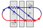
Figure 8: The first interference diagram of fig. 2, here showing how we label various energy fractions as $(x_{1},x_{2},x_{3},x_{4})$ following the convention of refs. qedNf . The shaded areas are discussed in the text.

In Zakharov’s formalism Zakharov1 ; Zakharov2 , this time-ordered diagram is evaluated by treating the gray regions as problems of 3- or 4-particle evolution in two-dimensional quantum mechanics, with an imaginary-valued potential that accounts for the effect of medium-averaged interactions of the high-energy particles with the medium. Those evolutions are then tied together with quantum field theory calculations of the vertices in fig. 8. In the case of 4-particle evolution (the middle gray area), the corresponding Hamiltonian is qedNf

$$\frac{({\bm{p}}_{1}^{\perp})^{2}}{2x_{1}E}+\frac{({\bm{p}}_{2}^{\perp})^{2}}{2x_{2}E}+\frac{({\bm{p}}_{3}^{\perp})^{2}}{2x_{3}E}+\frac{({\bm{p}}_{4}^{\perp})^{2}}{2x_{4}E}+V({\bm{b}}_{1},{\bm{b}}_{2},{\bm{b}}_{3},{\bm{b}}_{4})$$ (68a)

with potential

$$V({\bm{b}}_{1},{\bm{b}}_{2},{\bm{b}}_{3},{\bm{b}}_{4})=-\frac{i\hat{q}}{4}\left(b_{12}^{2}+b_{23}^{2}+b_{34}^{2}+b_{41}^{2}-b_{13}^{2}-b_{24}^{2}\right)=-\frac{i\hat{q}}{4}({\bm{b}}_{1}-{\bm{b}}_{2}+{\bm{b}}_{3}-{\bm{b}}_{4})^{2},$$ (68b)

where $({\bm{b}}_{1},{\bm{b}}_{2},{\bm{b}}_{3},{\bm{b}}_{4})$ are the transverse positions of the four particles, $({\bm{p}}_{1}^{\perp},{\bm{p}}_{2}^{\perp},{\bm{p}}_{3}^{\perp},{\bm{p}}_{4}^{\perp})$ are the corresponding transverse momenta, and ${\bm{b}}_{ij}\equiv{\bm{b}}_{i}-{\bm{b}}_{j}$. This Hamiltonian is not symmetric under exchanging the values of $x_{2}$ and $x_{3}$. However, the rate we are interested in calculating is invariant under (i) translations in the transverse plane and (ii) rotations that (at most) change the directions of the $z$ axis by a parametrically small amount (preserving the high-energy approximation that ${\bm{p}}^{\perp}\ll p^{z}$). This is enough symmetry to allow reduction of the 4-particle problem to an effective 2-particle problem with Hamiltonian

$$\frac{P_{41}^{2}}{2x_{1}x_{4}(x_{1}{+}x_{4})E}+\frac{P_{23}^{2}}{2x_{2}x_{3}(x_{2}{+}x_{3})E}-\frac{i\hat{q}}{4}(x_{1}{+}x_{4})^{2}\left({\bm{C}}_{41}-{\bm{C}}_{23}\right)^{2}$$ (69)

with degrees of freedom ${\bm{C}}_{41}$ and ${\bm{C}}_{23}$ defined by ${\bm{C}}_{ij}\equiv({\bm{b}}_{i}-{\bm{b}}_{j})/(x_{i}+x_{j})$ with conjugate momenta ${\bm{P}}_{ij}\equiv x_{j}{\bm{p}}_{i}^{\perp}-x_{i}{\bm{p}}_{j}^{\perp}$. The reduced Hamiltonian (69) is symmetric under exchanging the values of $x_{2}$ and $x_{3}$, which turns out to be the most critical reason that the final result will have that property. The other aspects of the problem can be mostly understood in terms of charge conjugation symmetry.

To see this, we should sketch a little more how the elements of the calculation fit together. The contribution from fig. 8 to the rate $\Delta\,d\Gamma/dx_{e}\,dx_{\scriptscriptstyle{{\rm E}}}$ was originally derived from a formula of the form qedNf ; seq

(splitting $$~{}\mbox{amplitude factors from the vertices)}\times\frac{N_{\rm f}\alpha^{2}}{(x_{1}{+}x_{4})^{2}}\int_{\rm times}\int_{{\bm{B}}^{\prime},{\bm{B}}^{\prime\prime}}$$

$$\times{\bm{\nabla}}_{{\bm{B}}^{\prime\prime\prime}}\langle{\bm{B}}^{\prime\prime\prime},t^{\prime\prime\prime}|{\bm{B}}^{\prime\prime},t^{\prime\prime}\rangle\Bigr{|}_{{\bm{B}}^{\prime\prime\prime}=0}$$

$$\times{\bm{\nabla}}_{{\bm{C}}^{\prime\prime}_{41}}{\bm{\nabla}}_{{\bm{C}}^{\prime}_{23}}\langle{\bm{C}}^{\prime\prime}_{41},{\bm{C}}^{\prime\prime}_{23},t^{\prime\prime}|{\bm{C}}^{\prime}_{41},{\bm{C}}^{\prime}_{23},t^{\prime}\rangle\Bigr{|}_{{\bm{C}}_{41}^{\prime\prime}=0={\bm{C}}_{23}^{\prime};~{}{\bm{C}}_{23}^{\prime\prime}={\bm{B}}^{\prime\prime};~{}{\bm{C}}_{41}^{\prime}={\bm{B}}^{\prime}}$$

$$\times{\bm{\nabla}}_{{\bm{B}}}\langle{\bm{B}}^{\prime},t^{\prime}|{\bm{B}},t\rangle\Bigr{|}_{{\bm{B}}=0}.$$ (70)

Above, the $\langle{\bm{C}}^{\prime\prime}_{41},{\bm{C}}^{\prime\prime}_{23},t^{\prime\prime}|{\bm{C}}^{\prime}_{41},{\bm{C}}^{\prime}_{23},t^{\prime}\rangle$ is the propagator associated with the Hamiltonian (69). The other two $\langle\cdots\rangle$’s are similar factors for the initial and final 3-particle evolution (leftmost and rightmost gray areas in fig. 8), where the same translation and rotational symmetries mentioned before have been used to reduce the problem from 3-particle quantum mechanics to effectively 1-particle quantum mechanics, with a variable we conventionally call ${\bm{B}}$ in the 3-particle case. Various separations ${\bm{B}}$ or ${\bm{C}}_{ij}$ are set to zero at vertices where two lines come together (and so their separation vanishes). The derivatives ${\bm{\nabla}}$ are position-space versions of transverse momentum factors associated with splitting vertices.

With (70) in hand, we sketch the other reasons for the $x_{2}{\leftrightarrow}x_{3}$ symmetry. (i) The expression only cares about the 4-particle propagator in terms of the variables ${\bm{C}}_{41}$ and ${\bm{C}}_{23}$, which is the choice of variables for which we noted (69) was $x_{2}{\leftrightarrow}x_{3}$ symmetric. (ii) The initial 3-particle evolution in fig. 8 (leftmost gray area) is independent of the values of $x_{2}$ and $x_{3}$. (iii) The final 3-particle evolution (of ${\rm E}$, ${\bar{\rm E}}$, and a conjugate-amplitude photon) is symmetric in $x_{2}{\leftrightarrow}x_{3}$ by charge conjugation invariance, and (iv) the vertices associated with $\gamma\to{\rm E}{\bar{\rm E}}$ at the start and end of the final 3-particle evolution come with amplitudes that are also symmetric by charge conjugation invariance.

Finally, the same style of argument can be used for the other large-$N_{\rm f}$ diagrams, including fig. 3, by labeling the particles in any 4-particle evolution the same way [$(x_{1},x_{2},x_{3},x_{4})=(-1,x_{\scriptscriptstyle{{\rm E}}},x_{\scriptscriptstyle{{\bar{\rm E}}}},x_{e})$] and then describing the 4-particle evolution with (69).

Appendix B DGLAP origin of logarithms $\ln x$ and $\ln(1{-}x)$ in eqs. (18) for $f_{i\to j}(x)$

To understand the coefficients of the logarithms in (18) for our NLO fit functions $f_{\underline{i\to j}}(x)$, we start by looking at the piece $f_{e\to e}^{\rm real}(x)$ (23a) of $f_{\underline{e\to e}}(x)$ that corresponds to real, double splitting $e\to e{\rm E}{\bar{\rm E}}$.

B.1 $e\to e{\rm E}{\bar{\rm E}}$

In this appendix, it will be convenient to use the notation shown in fig. 9 for the energies of particles in the $e{\to}e\gamma\to e{\rm E}{\bar{\rm E}}$ double splitting process. In particular, we introduce $E_{\gamma}$ as the energy of the intermediate photon and

$${\mathfrak{y}}_{\scriptscriptstyle{{\rm E}}}\equiv\frac{x_{\scriptscriptstyle{{\rm E}}}}{x_{\gamma}}=\frac{x_{\scriptscriptstyle{{\rm E}}}}{1{-}x_{e}}$$ (71)

as the energy fraction of the pair electron ${\rm E}$ relative to its immediate parent, the photon.

Figure 9: $e\to e{\rm E}{\bar{\rm E}}$ process

For what follows, it will be useful to have at hand parametric formulas for the formation times for individual, single splitting processes $e\to e\gamma$ and $\gamma\to{\rm E}{\bar{\rm E}}$:

$$t_{\rm form}^{e\to e\gamma} \sim\sqrt{\frac{x_{e}E}{x_{\gamma}\hat{q}}}=\sqrt{\frac{x_{e}E}{(1{-}x_{e})\hat{q}}}\,,$$ (72a)

$$t_{\rm form}^{\gamma\to{\rm E}{\bar{\rm E}}} \sim\sqrt{\frac{{\mathfrak{y}}_{\scriptscriptstyle{{\rm E}}}{\mathfrak{y}}_{\scriptscriptstyle{{\bar{\rm E}}}}E_{\gamma}}{\hat{q}}}=\sqrt{\frac{{\mathfrak{y}}_{\scriptscriptstyle{{\rm E}}}(1{-}{\mathfrak{y}}_{\scriptscriptstyle{{\rm E}}})(1{-}x_{e})E}{\hat{q}}}\,,$$ (72b)

coming from $t_{\rm form}\sim|\Omega|^{-1}$ and (25) [with $(x_{\scriptscriptstyle{{\rm E}}},x_{\scriptscriptstyle{{\bar{\rm E}}}},E)$ in (25c) replaced here by $({\mathfrak{y}}_{\scriptscriptstyle{{\rm E}}},{\mathfrak{y}}_{\scriptscriptstyle{{\bar{\rm E}}}},E_{\gamma})$].

B.1.1 $x_{e}\to 1$

In the limit $x_{e}\to 1$, (72) gives

$$t_{\rm form}^{\gamma\to{\rm E}{\bar{\rm E}}}\ll t_{\rm form}^{e\to e\gamma}.$$ (73)

The splitting with the smallest formation time is the one that most disrupts the LPM effect. Following the argument of appendix B.1 of ref. seq , we will treat the splitting with the parametrically smaller formation time (in this case $\gamma\to{\rm E}{\bar{\rm E}}$) as the “underlying” medium-induced splitting process, and we will treat the other splitting (here the earlier $e\to e\gamma$) as a vacuum-like DGLAP correction to that underlying process. Specifically, following through to eqs. (B.6) and (B.7) of ref. seq , we approximate

$$\left[\Delta\,\frac{d\Gamma}{dx_{e}\,d{\mathfrak{y}}_{\scriptscriptstyle{{\rm E}}}}\right]_{e\to e{\rm E}{\bar{\rm E}}}\approx\frac{\alpha}{2\pi}\,P_{e\to e}(x_{e})\,\ln\biggl{(}\frac{t_{\rm form}^{e\to e\gamma}}{t_{\rm form}^{\gamma\to{\rm E}{\bar{\rm E}}}}\biggr{)}\left[\frac{d\Gamma}{d{\mathfrak{y}}_{\scriptscriptstyle{{\rm E}}}}\right]^{\rm LO}_{\gamma\to{\rm E}{\bar{\rm E}}},$$ (74)

where $\approx$ indicates a leading-log approximation. Using (72), remembering that we are taking $x_{e}{\to}1$, and then integrating both sides with respect to ${\mathfrak{y}}_{\scriptscriptstyle{{\rm E}}}$ gives

$$\int_{0}^{1}d{\mathfrak{y}}_{\scriptscriptstyle{{\rm E}}}\>\left[\Delta\,\frac{d\Gamma}{dx_{e}\,d{\mathfrak{y}}_{\scriptscriptstyle{{\rm E}}}}\right]_{e\to e{\rm E}{\bar{\rm E}}}\approx\frac{\alpha}{2\pi}\,P_{e\to e}(x_{e})\,\ln\Bigl{(}\frac{1}{1{-}x_{e}}\Bigr{)}\,\Gamma^{\rm LO}_{\gamma\to{\rm E}{\bar{\rm E}}},$$ (75)

where, using (4b) and (5),

$$\Gamma^{\rm LO}_{\gamma\to{\rm E}{\bar{\rm E}}}=\frac{N_{\rm f}\alpha}{2\pi}\sqrt{\frac{\hat{q}}{E_{\gamma}}}\int_{0}^{1}d{\mathfrak{y}}_{\scriptscriptstyle{{\rm E}}}\>\frac{{\mathfrak{y}}_{\scriptscriptstyle{{\rm E}}}^{2}+(1{-}{\mathfrak{y}}_{\scriptscriptstyle{{\rm E}}})^{2}}{\sqrt{{\mathfrak{y}}_{\scriptscriptstyle{{\rm E}}}(1{-}{\mathfrak{y}}_{\scriptscriptstyle{{\rm E}}})}}=\frac{3N_{\rm f}\alpha}{8}\sqrt{\frac{\hat{q}}{E_{\gamma}}}.$$ (76)

Using this in (75), and taking the $x_{e}{\to}1$ limit of $P_{e\to e}(x)$ from (5),

$$\int_{0}^{1}d{\mathfrak{y}}_{\scriptscriptstyle{{\rm E}}}\>\left[\Delta\,\frac{d\Gamma}{dx_{e}\,d{\mathfrak{y}}_{\scriptscriptstyle{{\rm E}}}}\right]_{e\to e{\rm E}{\bar{\rm E}}}\approx-\frac{3N_{\rm f}\alpha^{2}}{8\pi}\,\frac{\ln(1{-}x_{e})}{(1{-}x_{e})^{3/2}}\sqrt{\frac{\hat{q}}{E}}\,.$$ (77)

The left-hand side above is equivalent (after changing variables) to the left-hand side of (22), and so $f_{e\to e}^{\rm real}(x_{e})$ is given by dividing (77) by the $R_{{\underline{e\to e}}}(x_{e})$ of (13a),

$$f_{e\to e}^{\rm real}(x_{e})\approx-\tfrac{3}{4}\ln(1{-}x_{e}).$$ (78)

This is the $\ln(1{-}x)$ term that we used in our fit (23a).

Readers not convinced by our fast and loose argument for (74) may be reassured to see numerical evidence that the coefficient on the logarithm in (78) has been correctly identified. Fig. 10b shows a log-linear plot of the numerical data points for $f_{e\to e}^{\rm real}(x)$ vs. $1{-}x$, arranged so that $x\simeq 1$ corresponds to the right-hand side of the plot. The coefficient of $\ln(1{-}x)$ is determined by the limit of the slope of this plot as $x\to 1$. To check the slope, we have also drawn a line

$$-\tfrac{3}{4}\ln(1{-}x_{e})+{\rm constant}$$ (79)

corresponding to the second term of our fit (23a) plus the (constant) $x_{e}\to 1$ limit of all the other terms. The slopes of that line and of the numerical data indeed match extremely well as $x\to 1$.

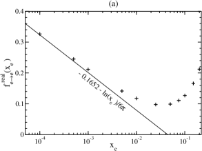
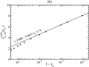
Figure 10: Log-linear plots of numerical results for $f_{e\to e}^{\rm real}(x_{e})$ vs. (a) $x_{e}$ and (b) $1{-}x_{e}$. The numerical data points ($+$) are taken from table 2 using (20). The points are compared to lines whose slopes on these plots correspond to our leading-log analytic results (a) $-\frac{1}{6\pi}\ln x$ and (b) $-\frac{3}{4}\ln(1{-}x_{e})$ for the limits $x_{e}\to 0$ and $x_{e}\to 1$ respectively. Note that the horizontal axis in both plots is oriented so that $x_{e}\to 0$ is toward the left and $x_{e}\to 1$ is toward the right.

B.1.2 $x_{e}\to 0$

In the limit $x_{e}\to 0$ with ${\mathfrak{y}}_{\scriptscriptstyle{{\rm E}}}$ held fixed, (72) gives

$$t_{\rm form}^{\gamma\to{\rm E}{\bar{\rm E}}}\gg t_{\rm form}^{e\to e\gamma},$$ (80)

and so, by the previous logic, we now consider $e\to e\gamma$ to be the underlying medium-induced splitting process, and $\gamma\to{\rm E}{\bar{\rm E}}$ is a vacuum-like fragmentation correction which can also be expressed as a DGLAP-like correction. The analog of (74) is

$$\left[\Delta\,\frac{d\Gamma}{dx_{e}\,d{\mathfrak{y}}_{\scriptscriptstyle{{\rm E}}}}\right]_{e\to e{\rm E}{\bar{\rm E}}}\approx\frac{\alpha}{2\pi}\,N_{\rm f}P_{\gamma\to e}({\mathfrak{y}}_{\scriptscriptstyle{{\rm E}}})\,\ln\biggl{(}\frac{t_{\rm form}^{\gamma\to{\rm E}{\bar{\rm E}}}}{t_{\rm form}^{e\to e\gamma}}\biggr{)}\left[\frac{d\Gamma}{dx_{e}}\right]^{\rm LO}_{e\to\gamma e},$$ (81)

from which

$$\int_{0}^{1}d{\mathfrak{y}}_{\scriptscriptstyle{{\rm E}}}\>\left[\Delta\,\frac{d\Gamma}{dx_{e}\,d{\mathfrak{y}}_{\scriptscriptstyle{{\rm E}}}}\right]_{e\to e{\rm E}{\bar{\rm E}}}\approx\frac{N_{\rm f}\alpha}{2\pi}\,\ln(x_{e}^{-1/2})\left[\frac{d\Gamma}{dx_{e}}\right]^{\rm LO}_{e\to\gamma e}\int_{0}^{1}d{\mathfrak{y}}_{\scriptscriptstyle{{\rm E}}}\>P_{\gamma\to e}({\mathfrak{y}}_{\scriptscriptstyle{{\rm E}}})\\ \simeq-\frac{N_{\rm f}\alpha^{2}}{12\pi^{2}}\,\frac{\ln x_{e}}{x_{e}^{1/2}}\sqrt{\frac{\hat{q}}{E}}\,.$$ (82)

Dividing by the $R_{{\underline{e\to e}}}(x_{e})$ of (13a) gives

$$f_{e\to e}^{\rm real}(x_{e})\approx-\tfrac{1}{6\pi}\ln x_{e},$$ (83)

which is the $\ln x$ term that we used in our fit (23a).

The a posteriori check that it was okay to take $x_{e}{\to}0$ in (80) while ignoring the possibility that ${\mathfrak{y}}_{e}$ or $1{-}{\mathfrak{y}}_{e}$ was also very small is that the ${\mathfrak{y}}_{\scriptscriptstyle{{\rm E}}}$ integral in (82) was convergent.

As a numerical check of (83), see fig. 10a. The line is

$$-\tfrac{1}{6\pi}\ln x_{e}+{\rm constant},$$ (84)

corresponding to the first term of (23a) plus the (constant) $x_{e}{\to}0$ limit of all the other terms.

B.1.3 $x_{\scriptscriptstyle{{\rm E}}}\to 0$

We now study the behavior of the NLO net rate $[d\Gamma/dx_{\scriptscriptstyle{{\rm E}}}]_{\underline{e\to{\rm E}}}^{\rm NLO}$ of (11b) as $x_{\scriptscriptstyle{{\rm E}}}\to 0$. Only the $e\to e{\rm E}{\bar{\rm E}}$ process contributes to that net rate. Consider now the limit $x_{\scriptscriptstyle{{\rm E}}}\to 0$ of the formation times (72). Throughout this discussion, we will take that limit while assuming that both ${\mathfrak{y}}_{\scriptscriptstyle{{\rm E}}}\equiv x_{\scriptscriptstyle{{\rm E}}}/(1{-}x_{e})$ and $1{-}{\mathfrak{y}}_{\scriptscriptstyle{{\rm E}}}$ remain $O(1)$, and so $1{-}x_{e}=O(x_{\scriptscriptstyle{{\rm E}}})$ and $x_{e}\to 1$. The a posteriori justification is that we will encounter no divergence when we later integrate over ${\mathfrak{y}}_{\scriptscriptstyle{{\rm E}}}$ in this approximation.

The limit $x_{\scriptscriptstyle{{\rm E}}}\to 0$ ($x_{e}\to 1$) of (72) therefore gives us the same hierarchy of formation times as (73), and so we have the same leading-log approximation (74) for $[\Delta\,d\Gamma/dx_{e}\,d{\mathfrak{y}}_{\scriptscriptstyle{{\rm E}}}]_{e\to e{\rm E}{\bar{\rm E}}}$. The $x_{e}{\to}1$ limit of (74) is the unintegrated version of (75):

$$\left[\Delta\,\frac{d\Gamma}{dx_{e}\,d{\mathfrak{y}}_{\scriptscriptstyle{{\rm E}}}}\right]_{e\to e{\rm E}{\bar{\rm E}}}\approx\frac{\alpha}{2\pi}\,P_{e\to e}(x_{e})\,\ln\Bigl{(}\frac{1}{1{-}x_{e}}\Bigr{)}\left[\frac{d\Gamma}{d{\mathfrak{y}}_{\scriptscriptstyle{{\rm E}}}}\right]^{\rm LO}_{\gamma\to{\rm E}{\bar{\rm E}}}\!\!({\mathfrak{y}}_{\scriptscriptstyle{{\rm E}}},E_{\gamma}),$$ (85)

where we find it useful to now explicitly list the momentum fraction and energy arguments appropriate for the LO $\gamma\to{\rm E}{\bar{\rm E}}$ rate. The difference here will be in how we then integrate to get $[d\Gamma/dx_{\scriptscriptstyle{{\rm E}}}]^{\rm NLO}_{\underline{e\to{\rm E}}}$ instead of the behavior of the real double splitting contribution (22) to the net rate $[d\Gamma/dx_{e}]^{\rm NLO}_{\underline{e\to e}}$.

Use the definition (71) of ${\mathfrak{y}}_{\scriptscriptstyle{{\rm E}}}$ to change variables from $(x_{e},{\mathfrak{y}}_{\scriptscriptstyle{{\rm E}}})$ to $(x_{\scriptscriptstyle{{\rm E}}},{\mathfrak{y}}_{\scriptscriptstyle{{\rm E}}})$,

$$\left[\Delta\,\frac{d\Gamma}{dx_{\scriptscriptstyle{{\rm E}}}\,d{\mathfrak{y}}_{\scriptscriptstyle{{\rm E}}}}\right]_{e\to e{\rm E}{\bar{\rm E}}}\approx\frac{\alpha}{2\pi{\mathfrak{y}}_{\scriptscriptstyle{{\rm E}}}}\,P_{e\to e}\bigl{(}1-\tfrac{x_{\scriptscriptstyle{{\rm E}}}}{{\mathfrak{y}}_{\scriptscriptstyle{{\rm E}}}}\bigr{)}\,\ln\Bigl{(}\frac{{\mathfrak{y}}_{\scriptscriptstyle{{\rm E}}}}{x_{\scriptscriptstyle{{\rm E}}}}\Bigr{)}\left[\frac{d\Gamma}{d{\mathfrak{y}}_{\scriptscriptstyle{{\rm E}}}}\right]^{\rm LO}_{\gamma\to{\rm E}{\bar{\rm E}}}\!\!\bigl{(}{\mathfrak{y}}_{\scriptscriptstyle{{\rm E}}},\tfrac{x_{\scriptscriptstyle{{\rm E}}}}{{\mathfrak{y}}_{\scriptscriptstyle{{\rm E}}}}E\bigr{)}.$$ (86a)

With these variables, the NLO net rate for $$e\to{\rm E}$$ is given by the integral

$$\left[\frac{d\Gamma}{dx_{\scriptscriptstyle{{\rm E}}}}\right]^{\rm NLO}_{\underline{e\to{\rm E}}}=\int_{x_{\scriptscriptstyle{{\rm E}}}}^{1}d{\mathfrak{y}}_{\scriptscriptstyle{{\rm E}}}\>\left[\Delta\,\frac{d\Gamma}{dx_{\scriptscriptstyle{{\rm E}}}\,d{\mathfrak{y}}_{\scriptscriptstyle{{\rm E}}}}\right]_{e\to e{\rm E}{\bar{\rm E}}}.$$ (86b)

Taking $x_{\scriptscriptstyle{{\rm E}}}\to 0$ while treating ${\mathfrak{y}}_{\scriptscriptstyle{{\rm E}}}$ as $O(1)$, (86) gives

$$\left[\frac{d\Gamma}{dx_{\scriptscriptstyle{{\rm E}}}}\right]^{\rm NLO}_{\underline{e\to{\rm E}}}\approx-\frac{N_{\rm f}\alpha^{2}}{2\pi^{2}}\,\frac{\ln x_{\scriptscriptstyle{{\rm E}}}}{x_{\scriptscriptstyle{{\rm E}}}^{3/2}}\sqrt{\frac{\hat{q}}{E}}\int_{0}^{1}d{\mathfrak{y}}_{\scriptscriptstyle{{\rm E}}}\>\frac{{\mathfrak{y}}_{\scriptscriptstyle{{\rm E}}}^{2}+(1{-}{\mathfrak{y}}_{\scriptscriptstyle{{\rm E}}})^{2}}{\sqrt{1-{\mathfrak{y}}_{\scriptscriptstyle{{\rm E}}}}}\simeq-\frac{11\,N_{\rm f}\alpha^{2}}{15\pi^{2}}\,\frac{\ln x_{\scriptscriptstyle{{\rm E}}}}{x_{\scriptscriptstyle{{\rm E}}}^{3/2}}\sqrt{\frac{\hat{q}}{E}}$$ (87)

as in (18b). Finally, dividing by the corresponding $R_{\underline{e\to{\rm E}}}(x_{\scriptscriptstyle{{\rm E}}})$ of (13b),

$$f_{\underline{e\to{\rm E}}}(x_{\scriptscriptstyle{{\rm E}}})\approx-\tfrac{22}{15\pi}\ln x_{\scriptscriptstyle{{\rm E}}}.$$ (88)

A numerical check of this result is shown in fig. 11a.

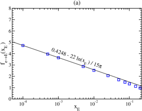
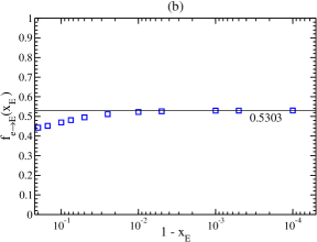
Figure 11: Like fig. 10 but here log-linear plots of numerical results for $f_{\underline{e\to{\rm E}}}(x_{\scriptscriptstyle{{\rm E}}})$ vs. (a) $x_{\scriptscriptstyle{{\rm E}}}$ and (b) $1{-}x_{\scriptscriptstyle{{\rm E}}}$.

B.1.4 $x_{\scriptscriptstyle{{\rm E}}}\to 1$

The limit $x_{\scriptscriptstyle{{\rm E}}}\to 1$ requires both $x_{e}\to 0$ and $x_{\scriptscriptstyle{{\bar{\rm E}}}}\to 0$. If we assume $x_{e}\sim x_{\scriptscriptstyle{{\bar{\rm E}}}}$, then (72) does not give any hierarchy of formation times:

$$t_{\rm form}^{\gamma\to{\rm E}{\bar{\rm E}}}\sim t_{\rm form}^{e\to e\gamma}.$$ (89)

No hierarchy suggest no logarithmic enhancement, and so we might expect $f_{\underline{e\to{\rm E}}}(x_{\scriptscriptstyle{{\rm E}}})$ to have no $\ln(1{-}x_{\scriptscriptstyle{{\rm E}}})$ behavior as $x_{\scriptscriptstyle{{\rm E}}}\to 1$:

$$f_{\underline{e\to{\rm E}}}(x_{\scriptscriptstyle{{\rm E}}})\to{\rm constant}.$$ (90)

We verify this expectation in fig. 11b, where we compare numerical results to the constant taken from the $x_{\scriptscriptstyle{{\rm E}}}{\to}1$ limit of our fit (18b).

B.2 Virtual diagrams

We do not have a method for deducing ab initio the logarithmic behavior of $f_{{\underline{i\to j}}}$’s that contain virtual diagrams. Here, we will rely on numerics to identify which limits lack any logarithmic terms $\ln x$ or $\ln(1{-}x)$. We will then be able to combine those cases with the previous $e\to e{\rm E}{\bar{\rm E}}$ results for $f^{\rm real}_{e\to e}(x_{e})$ to determine the remaining logarithms in (18) and (23b).

Fig. 12a shows the $x{\to}0$ behavior of our numerical results for $f_{\underline{e\to e}}(x)$, $f_{\underline{e\to\gamma}}(x)$, and $f_{\underline{\gamma\to{\rm E}}}(x)$, and the horizontal lines show the constants given by the $x{\to}0$ limit of the corresponding fit functions in (18). It is clear from the plot that the numerical data points for $f_{\underline{e\to e}}(x)$ and $f_{\underline{\gamma\to{\rm E}}}(x)$ approach a constant as $x\to 0$, and there is no sign of any $\ln x$ behavior. By (20), this also means that $f_{e\to e}^{\rm virt}(x)$ has no $\ln(1{-}x)$ behavior, as in (23b).

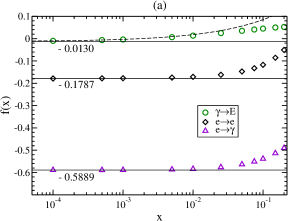
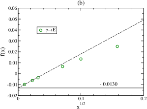
Figure 12: (a) Like fig. 10a but here for log-linear plots of numerical results for $f_{\underline{e\to e}}(x)$, $f_{\underline{e\to\gamma}}(x)$, and $f_{\underline{\gamma\to{\rm E}}}(x)$ vs. $x$. The dashed curve is $-0.0130+0.3106\sqrt{x}$ as in (91). (b) A linear plot of $f_{\underline{\gamma\to{\rm E}}}(x)$ vs. $\sqrt{x}$.

The case of $f_{\underline{\gamma\to{\rm E}}}(x)$ is less clear; visually, it is hard to determine from fig. 12a whether the slope of the numerical data is definitely approaching zero as $x\to 0$. However, as noted in ref. finale2 , expansions can be in $\sqrt{x}$ rather than $x$, as was reflected in the form of our fit functions (18). For (18d), the first two terms in the expansion of the fit for small $x$ are

$$f_{\underline{\gamma\to{\rm E}}}(x_{\gamma})\simeq-0.0130+0.3106\sqrt{x_{\gamma}},$$ (91)

represented by the dashed curve in fig. 12. The slow convergence of the ${\underline{\gamma\to{\rm E}}}$ data points to a constant in fig. 12a is consistent with the presence of a $\sqrt{x}$ correction, which is made clearer by fig. 12b, where $f_{\underline{\gamma\to{\rm E}}}(x)$ is plotted vs. $\sqrt{x}$. There is no evidence of $\ln x$ behavior. Since $f_{\underline{\gamma\to{\rm E}}}(x)$ is symmetric under $x\to 1{-}x$ by charge conjugation, this also means that there is no $\ln(1{-}x)$ behavior.

We now have enough information to reconstruct other limits. From (19) and (20), we have

$$f_{\underline{e\to e}}(x_{e})=f_{\underline{e\to\gamma}}(1{-}x_{e})+f_{e\to e}^{\rm real}(x_{e}).$$ (92)

Combined with our numerical result that $f_{\underline{e\to\gamma}}(x_{\gamma})$ approaches a constant as $x_{\gamma}\to 0$ and that $f_{e\to e}^{\rm real}(x_{e})$ behaves like (78) as $x_{e}\to 1$, we get

$$f_{\underline{e\to e}}(x_{e})\approx f_{e\to e}^{\rm real}(x_{e})\approx-\tfrac{3}{4}\ln(1{-}x_{e})~{}~{}\mbox{for}~{}~{}x_{e}\to 1,$$ (93)

which is what we used in the fit (18a).

Similarly, eq. (19) plus our numerical result that $f_{\underline{e\to e}}(x_{e})$ approaches a constant as $x_{e}\to 0$ gives $f_{e\to e}^{\rm virt}(x_{e})\approx-f_{e\to e}^{\rm real}(x_{e})$ for $x_{e}\to 0$, and then (83) gives

$$f_{e\to e}^{\rm virt}(x_{e})\approx\tfrac{1}{6\pi}\ln x_{e}~{}~{}\mbox{for}~{}~{}x_{e}\to 0$$ (94)

as in (23b).

Appendix C Parametric estimate of $(p_{2}{+}p_{3})^{\mu}(p_{2}{+}p_{3})_{\mu}$

In (28), we asserted that parametrically $(p_{2}{+}p_{3})^{\mu}(p_{2}{+}p_{3})_{\mu}\sim E/t_{\rm form}$ for a leading-order BDMPS-Z single splitting where the two daughters have momenta $p_{2}$ and $p_{3}$. A mnemonic for remembering this formula is to remember that, in the case of a single virtual particle, its virtuality is $P^{\mu}P_{\mu}\simeq 2E\Delta E$ when the particle is off-shell in energy by $\Delta E\ll E$. If we uncritically use that same formula in our case and interpret $E$ as the energy of the parent and $\Delta E$ as the typical off-shellness of the splitting process during the formation time, then we can use the uncertainty relation $\Delta E\sim 1/\Delta t$ to guess (28).

In this appendix, we want to be more concrete by keeping all of the argument specific to the case of BDMPS-Z splitting. The splitting process is high energy and nearly collinear in the frame we usually work in, the rest frame of the medium. So we can approximate the 4-momenta of each on-shell daughter as

$$(p_{i}^{0},{\bm{p}}_{i}^{\perp},p_{i}^{z})\simeq\left(x_{i}E+\frac{(p^{\perp}_{i})^{2}}{2x_{i}E}\,,\,{\bm{p}}^{\perp}_{i}\,,\,x_{i}E\right),$$ (95)

where for this purpose we define $x_{i}$ as the $p^{z}$ fraction relative to the parent, and we use $({+}{-}{-}{-})$ metric convention. Then, in the high-energy approximation,

$$(p_{2}{+}p_{3})^{\mu}(p_{2}{+}p_{3})_{\mu}=2p_{2}^{\mu}p_{3\mu}\simeq\frac{(x_{3}{\bm{p}}^{\perp}_{2}-x_{2}{\bm{p}}^{\perp}_{3})^{2}}{x_{2}x_{3}}.$$ (96a)

The combination

$${\bm{P}}^{\perp}\equiv x_{3}{\bm{p}}^{\perp}_{2}-x_{2}{\bm{p}}^{\perp}_{3}$$ (96b)

is invariant under rotations that preserve the high-energy approximation $p_{i}^{\perp}\ll p_{i}^{z}$. In the $\hat{q}$ approximation, solving the single splitting BDMPS-Z problem involves solving a two-dimensional non-Hermitian harmonic oscillator problem with Hamiltonian

$${\cal H}=\frac{(P^{\perp})^{2}}{2M}+\frac{1}{2}M\Omega^{2}B^{2},$$ (97)

where ${\bm{B}}\equiv{\bm{b}}_{2}-{\bm{b}}_{3}$ is the separation of the two daughters in the transverse plane and is conjugate to ${\bm{P}}^{\perp}$; $\Omega$ above is given by (25); and $M\equiv x_{2}x_{3}E$. In the form introduced by Zakharov Zakharov1 ; Zakharov2 , the leading-order splitting rate (in an infinite medium) is then given in terms of the propagator $\langle{\bm{B}},t|{\bm{B}}^{\prime},t^{\prime}\rangle$ of the above harmonic oscillator by

$$\frac{d\Gamma}{dx}=\frac{\alpha P(x)}{M^{2}}\operatorname{Re}\int_{0}^{\infty}d(\Delta t)\>{\bm{\nabla}}_{{\bm{B}}}\cdot{\bm{\nabla}}_{{\bm{B}}^{\prime}}\langle{\bm{B}},\Delta t|{\bm{B}}^{\prime},0\rangle\Bigr{|}_{{\bm{B}}={\bm{B}}^{\prime}=0},$$ (98)

where $P(x)$ is the relevant DGLAP vacuum splitting function, $\Delta t$ is the duration of the splitting process, and the $\Delta t$ integral is dominated by $\Delta t\sim t_{\rm form}\sim 1/|\Omega|$. During the formation time, the typical size of ${\cal H}$ is parametrically $1/t_{\rm form}\sim|{\cal H}|\sim(P^{\perp})^{2}/2M$, and so $(P^{\perp})^{2}\sim M/t_{\rm form}=x_{2}x_{3}E/t_{\rm form}$. Using (96) then gives the promised parametric estimate (28).

Appendix D Another path to the large-$N_{\rm f}$ recursion relations for $\langle z^{n}\rangle_{\epsilon,i}$

In this appendix, we discuss another way that one can arrive at the large-$N_{\rm f}$ recursion relations (66), by taking the large-$N_{\rm f}$ limit at the beginning of the derivation.

D.1 $e^{\pm}$ evolution

Because the $e\to e\gamma$ rate is suppressed by a factor of $N_{\rm f}^{-1}$ compared to the $\gamma\to{\rm E}{\bar{\rm E}}$ rate, it is the $e\to e\gamma$ rate that will be the bottleneck to shower development and so will parametrically determine the stopping length (and other moments) for charge and energy deposition. This hierarchy of scales is depicted in fig. 13. In the large-$N_{\rm f}$ limit, the lifetime of photons in the in-medium shower is negligible compared to the duration of the shower, and so we may always treat the combination $e\to e\gamma\to e{\rm E}{\bar{\rm E}}$ of $e\to e\gamma$ and $\gamma\to{\rm E}{\bar{\rm E}}$ splittings as effectively instantaneous, even for the case of non-overlapping splittings. When overlap effects are ignored, the combined rate for such a sequential splitting would be (i) the rate for the initial $e\to e\gamma$ splitting multiplied by (ii) the probability distribution for energy fractions of the subsequent, inevitable $\gamma\to{\rm E}{\bar{\rm E}}$ splitting a moment later:

$$\left[\frac{d\Gamma}{dx_{e}\,d{\mathfrak{y}}_{\scriptscriptstyle{{\rm E}}}}(E)\right]^{\rm indep}_{e\to e{\rm E}{\bar{\rm E}}}\equiv\left[\frac{d\Gamma}{dx_{e}}(E)\right]_{e\to e\gamma}\!\times\frac{1}{\Gamma_{\gamma}\bigl{(}(1{-}x_{e})E\bigr{)}}\,\left[\frac{d\Gamma}{d{\mathfrak{y}}_{\scriptscriptstyle{{\rm E}}}}\bigl{(}(1{-}x_{e})E\bigr{)}\right]_{\gamma\to{\rm E}{\bar{\rm E}}},$$ (99a)

where $${\mathfrak{y}}_{\scriptscriptstyle{{\rm E}}} {\rm E} \gamma$$ is the energy fraction (71) of the final pair electron () relative to its immediate parent . Note that

$$\left[\frac{d\Gamma}{dx_{e}\,dx_{\scriptscriptstyle{{\rm E}}}}(E)\right]^{\rm indep}_{e\to e{\rm E}{\bar{\rm E}}}=\frac{1}{(1{-}x_{e})}\left[\frac{d\Gamma}{dx_{e}\,d{\mathfrak{y}}_{\scriptscriptstyle{{\rm E}}}}(E)\right]^{\rm indep}_{e\to e{\rm E}{\bar{\rm E}}}.$$ (99b)

The superscript “${\rm indep}$” in (99a) means “independent” and indicates that the possibility that $e\to e\gamma$ and $\gamma\to{\rm E}{\bar{\rm E}}$ overlap each other has been ignored. However, we do include virtual NLO corrections to each individual splitting. That is, the single-splitting rates appearing on the right-hand side of (99a) are each the sum of LO+NLO single-splitting rates as in (8a) and (8b), and similarly for the total single-splitting rate $\Gamma_{\gamma}$ in the denominator.

We can now undo the approximation that $e\to e\gamma$ and $\gamma\to{\rm E}{\bar{\rm E}}$ do not overlap by adding in the known overlap correction $[\Delta d\Gamma/dx_{e}\,dx_{\scriptscriptstyle{{\rm E}}}]_{e\to e{\rm E}{\bar{\rm E}}}$. This will allow us to describe shower development in the large-$N_{\rm f}$ limit using just one rate, which we will call the super-effective $1{\to}3$ rate:

$$\left[\frac{d\Gamma}{dx_{e}\,dx_{\scriptscriptstyle{{\rm E}}}}\right]^{\rm super}_{e\to e{\rm E}{\bar{\rm E}}}\equiv\left[\frac{d\Gamma}{dx_{e}\,dx_{\scriptscriptstyle{{\rm E}}}}\right]^{\rm indep}_{e\to e{\rm E}{\bar{\rm E}}}+\left[\frac{\Delta\,d\Gamma}{dx_{e}\,dx_{\scriptscriptstyle{{\rm E}}}}\right]_{e\to e{\rm E}{\bar{\rm E}}}\,,$$ (100)

depicted pictorially in fig. 14. The analog of the net $e{\to}e^{\pm}$ rate given by (54a) is

$$\left[\frac{d\Gamma}{dx}\right]^{\begin{subarray}{c}{\rm super}\\ {\rm net}\end{subarray}}_{e\to e^{\pm}}\equiv\int_{0}^{1-x}dy\>\biggl{\{}\frac{d\Gamma^{\rm super}_{{e\to e{\scriptscriptstyle{{\rm E}}}{\scriptscriptstyle{{\bar{\rm E}}}}}}}{dx_{e}\,dx_{\scriptscriptstyle{{\rm E}}}}(x,y)+\frac{d\Gamma^{\rm super}_{{e\to e{\scriptscriptstyle{{\rm E}}}{\scriptscriptstyle{{\bar{\rm E}}}}}}}{dx_{e}\,dx_{\scriptscriptstyle{{\rm E}}}}(y,x)+\frac{d\Gamma^{\rm super}_{{e\to e{\scriptscriptstyle{{\rm E}}}{\scriptscriptstyle{{\bar{\rm E}}}}}}}{dx_{e}\,dx_{\scriptscriptstyle{{\rm E}}}}(y,1{-}x{-}y)\biggr{\}}.$$ (101)

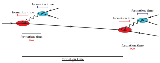
Figure 13: Hierarchy of scales in large-$N_{\rm f}$ QED qedNfstop .

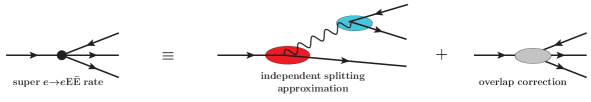
Figure 14: Definition (100) of the “super” $e{\to}e{\rm E}{\bar{\rm E}}$ rate, where all intermediate photons have been integrated out in $e\to e\gamma\to e{\rm E}{\bar{\rm E}}$, regardless of whether or not the two splittings $e\to e\gamma$ and $\gamma\to{\rm E}{\bar{\rm E}}$ overlap. Above, each picture of a diagram is meant to schematically represent its corresponding contribution to rates (not amplitudes), and it is rate contributions that are added.

The now purely-$e^{\pm}$ energy deposition equation is

$$\frac{\partial\epsilon_{e}(E,z)}{\partial z}=\int_{0}^{1}dx\>\left[\frac{d\Gamma}{dx}(E,x)\right]^{\begin{subarray}{c}{\rm super}\\ {\rm net}\end{subarray}}_{e\to e^{\pm}}\left\{\epsilon_{e}(xE,z)-x\epsilon_{e}(E,z)\right\},$$ (102)

which is the analog here of (53a). Assuming $E^{-1/2}$ scaling of rates, this gives

$$\frac{\partial\epsilon_{e}(z)}{\partial z}=\int_{0}^{1}dx\>x\left[\frac{d\Gamma}{dx}(E_{0},x)\right]^{\begin{subarray}{c}{\rm super}\\ {\rm net}\end{subarray}}_{e\to e^{\pm}}\left\{x^{-1/2}\epsilon_{e}(x^{-1/2}z)-\epsilon_{e}(z)\right\}.$$ (103)

Taking moments gives the recursion relation

$$-n\langle z^{n-1}\rangle_{\epsilon,e}=\int_{0}^{1}dx\>x\left[\frac{d\Gamma}{dx}(E_{0},x)\right]^{\rm net}_{e\to e^{\pm}}\left\{x^{n/2}\langle z^{n}\rangle_{\epsilon,e}-\langle z^{n}\rangle_{\epsilon,e}\right\}$$ (104)

and so

$$\langle z^{n}\rangle_{\epsilon,e}=n\mu^{-1}_{(n)}\langle z^{n-1}\rangle_{\epsilon,e}$$ (105a)

with the number

$$\mu_{(n)}\equiv\int_{0}^{1}dx\>x\left[\frac{d\Gamma}{dx}(E_{0},x)\right]^{{\begin{subarray}{c}{\rm super}\\ {\rm net}\end{subarray}}}_{e\to e^{\pm}}\{1-x^{n/2}\}=\operatorname{Avg}^{{\rm super},{\rm net}}_{e\to e^{\pm}}[x(1-x^{n/2})].$$ (105b)

This must be equivalent to the recursion relation (66a) derived for $\langle z^{n}\rangle_{\epsilon,e}$ in the main text, which means that

$$\operatorname{Avg}^{{\rm super},{\rm net}}_{e\to e^{\pm}}[x(1-x^{n/2})]=\frac{\det M_{(n)}}{M_{(n),\gamma\gamma}}\,.$$ (106)

Eq. (106) is not obvious from the formulas for its left-hand and right-hand sides, and so we will show how to verify it in section D.3 below.

D.2 Photon initiated showers

For a photon initiated shower, we may again make use of the fact that, in the large-$N_{\rm f}$ limit, the photon pair-produces instantly relative to the duration of the shower. That means that rather than an evolution equation (50b), we may just write an instantaneous relation,

$$\epsilon_{\gamma}(E,z)=\frac{1}{\Gamma_{\gamma}(E)}\left(\int_{0}^{1}dx\>\left[\frac{d\Gamma}{dx}(E,x)\right]^{\rm net}_{\underline{\gamma\to{\rm E}}}\,\epsilon_{e}(xE,z)+\int_{0}^{1}dx\>\left[\frac{d\Gamma}{dx}(E,x)\right]^{\rm net}_{\underline{\gamma\to{\bar{\rm E}}}}\,\epsilon_{e}(xE,z)\right)\\ =\frac{1}{\Gamma_{\gamma}(E)}\int_{0}^{1}dx\>\left[\frac{d\Gamma}{dx}(E,x)\right]^{\rm net}_{\gamma\to e^{\pm}}\,\epsilon_{e}(xE,z).$$ (107)

Assuming $E^{-1/2}$ scaling of the rates, this gives

$$\epsilon_{\gamma}(z)=\frac{1}{\Gamma_{\gamma}(E_{0})}\int_{0}^{1}dx\>x\left[\frac{d\Gamma}{dx}(E_{0},x)\right]^{\rm net}_{\gamma\to e^{\pm}}\left\{x^{-1/2}\epsilon_{e}(x^{-1/2}z)\right\},$$ (108)

and taking moments yields the same relation (66b) between $\langle z^{n}\rangle_{\epsilon,\gamma}$ and $\langle z^{n}\rangle_{\epsilon,e}$ that was derived in the main text.

D.3 Verifying eq. (106)

Now we discuss how to directly verify the relation (106) rather than merely asserting that it must be true. We find it convenient to rewrite the relation as

$$M_{ee}-\frac{M_{e\gamma}M_{\gamma e}}{M_{\gamma\gamma}}\overset{?}{=}\operatorname{Avg}^{{\rm super},{\rm net}}_{e\to e^{\pm}}[x(1-x^{n/2})],$$ (109)

where the question mark over an equality indicates an assertion that is being checked. To reduce notational clutter, in this section we abbreviate $M_{(n)}$ as $M$.

Consider the overlap correction $[\Delta\,d\Gamma/dx_{e}\,x_{\scriptscriptstyle{{\rm E}}}]_{e\to e{\rm E}{\bar{\rm E}}}$ to double splitting $e\to e\gamma\to e{\rm E}{\bar{\rm E}}$. On the left-hand side of (109), that overlap correction contributes only to the first term of

$$M_{ee}\equiv\operatorname{Avg}_{e\to e^{\pm}}\bigl{[}x{-}x^{1+\frac{n}{2}}\bigr{]}+\operatorname{Avg}_{e\to\gamma}\bigl{[}x]$$ (110)

[see (61)] and not to any of the other $M_{ij}$. Given the definitions of $[d\Gamma/dx]^{\rm net}_{e\to e^{\pm}}$ and $[d\Gamma/dx]^{{\rm super},{\rm net}}_{e\to e^{\pm}}$, that very same contribution also appears on the right-hand side of (109). So what remains is that we need to check the equality (109) for everything that’s not a double-splitting overlap correction. That’s

$$M_{ee}^{1\to 2}-\frac{M_{e\gamma}M_{\gamma e}}{M_{\gamma\gamma}}\overset{?}{=}\int_{0}^{1}dx\>\left[\frac{d\Gamma}{dx}\right]^{{\rm indep},{\rm net}}_{e\to e^{\pm}}x(1-x^{n/2}),$$ (111)

where

$$M^{1\to 2}_{ee}\equiv\operatorname{Avg}_{e\to e\gamma}\bigl{[}x_{e}-x_{e}^{1+\frac{n}{2}}\bigr{]}+\operatorname{Avg}_{e\to e\gamma}\bigl{[}x_{\gamma}],$$ (112)

which represents the contribution to the original $M_{ee}$ (110) from just the LO+NLO $1{\to}2$ process $e{\to}e\gamma$ but not from the effective $1{\to}3$ rate $[\Delta\,d\Gamma/dx_{e}\,x_{\scriptscriptstyle{{\rm E}}}]_{e\to e{\rm E}{\bar{\rm E}}}$ representing the overlap correction to $e\to e\gamma\to e{\rm E}{\bar{\rm E}}$. Note that every $M_{ij}$ on the left-hand side of (111) now only involves LO+NLO $1{\to}2$ processes. On the right-hand side of (111),

$$\left[\frac{d\Gamma}{dx}\right]^{\begin{subarray}{c}{\rm indep}\\ {\rm net}\end{subarray}}_{e\to e^{\pm}}\equiv\int_{0}^{1-x}dy\>\biggl{\{}\frac{d\Gamma^{\rm indep}_{{e\to e{\scriptscriptstyle{{\rm E}}}{\scriptscriptstyle{{\bar{\rm E}}}}}}}{dx_{e}\,dx_{\scriptscriptstyle{{\rm E}}}}(x,y)+\frac{d\Gamma^{\rm indep}_{{e\to e{\scriptscriptstyle{{\rm E}}}{\scriptscriptstyle{{\bar{\rm E}}}}}}}{dx_{e}\,dx_{\scriptscriptstyle{{\rm E}}}}(y,x)+\frac{d\Gamma^{\rm indep}_{{e\to e{\scriptscriptstyle{{\rm E}}}{\scriptscriptstyle{{\bar{\rm E}}}}}}}{dx_{e}\,dx_{\scriptscriptstyle{{\rm E}}}}(y,1{-}x{-}y)\biggr{\}},$$ (113)

analogous to (101), and recall that the “independent splitting” rate (99) was also defined exclusively in terms of LO+NLO $1{\to}2$ splitting processes.

Our next step is to realize that $x_{e}{+}x_{\gamma}=1$ for $e\to e\gamma$, and so (112) is

$$M^{1\to 2}_{ee}=\operatorname{Avg}_{e\to e\gamma}\bigl{[}x_{e}{+}x_{\gamma}\bigr{]}-\operatorname{Avg}_{e\to e\gamma}\bigl{[}x_{e}^{1+\frac{n}{2}}\bigr{]}=\Gamma_{e\to e\gamma}-\operatorname{Avg}_{e\to e\gamma}\bigl{[}x_{e}^{1+\frac{n}{2}}\bigr{]}.$$ (114)

There is a similar $\Gamma_{e\to e\gamma}$ term hiding in the $n$-independent term on the right-hand side of (111). Specifically,

$$\int_{0}^{1}dx\>x \left[\frac{d\Gamma}{dx}\right]^{{\rm indep},{\rm net}}_{e\to e^{\pm}}$$

$$=\int_{0}^{1}dx\>\int_{0}^{1-x}dy\>x\biggl{\{}\frac{d\Gamma^{\rm indep}_{{e\to e{\scriptscriptstyle{{\rm E}}}{\scriptscriptstyle{{\bar{\rm E}}}}}}}{dx_{e}dy_{\scriptscriptstyle{{\rm E}}}}(x,y)+\frac{d\Gamma^{\rm indep}_{{e\to e{\scriptscriptstyle{{\rm E}}}{\scriptscriptstyle{{\bar{\rm E}}}}}}}{dx_{e}dy_{\scriptscriptstyle{{\rm E}}}}(y,x)+\frac{d\Gamma^{\rm indep}_{{e\to e{\scriptscriptstyle{{\rm E}}}{\scriptscriptstyle{{\bar{\rm E}}}}}}}{dx_{e}dy_{\scriptscriptstyle{{\rm E}}}}(y,1{-}x{-}y)\biggr{\}}$$

$$=\int_{0}^{1}dx_{e}\>\int_{0}^{1-x_{e}}dx_{\scriptscriptstyle{{\rm E}}}\>(x_{e}+x_{\scriptscriptstyle{{\rm E}}}+x_{\scriptscriptstyle{{\bar{\rm E}}}})\,\frac{d\Gamma^{\rm indep}_{{e\to e{\scriptscriptstyle{{\rm E}}}{\scriptscriptstyle{{\bar{\rm E}}}}}}}{dx_{e}dx_{\scriptscriptstyle{{\rm E}}}}(x_{e},x_{\scriptscriptstyle{{\rm E}}})$$

$$=\Gamma^{\rm indep}_{{e\to e{\scriptscriptstyle{{\rm E}}}{\scriptscriptstyle{{\bar{\rm E}}}}}}$$

$$=\int_{0}^{1}dx_{e}\>\int_{0}^{1}d{\mathfrak{y}}_{\scriptscriptstyle{{\rm E}}}\left[\frac{d\Gamma}{dx_{e}}(E)\right]_{e\to e\gamma}\,\frac{1}{\Gamma_{\gamma}\bigl{(}(1{-}x_{e})E\bigr{)}}\,\left[\frac{d\Gamma}{d{\mathfrak{y}}_{\scriptscriptstyle{{\rm E}}}}\bigl{(}(1{-}x_{e})E\bigr{)}\right]_{\gamma\to{\rm E}{\bar{\rm E}}}$$

$$=\int_{0}^{1}dx_{e}\>\left[\frac{d\Gamma}{dx_{e}}(E)\right]_{e\to e\gamma}\,\frac{1}{\Gamma_{\gamma}\bigl{(}(1{-}x_{e})E\bigr{)}}\int_{0}^{1}d{\mathfrak{y}}_{\scriptscriptstyle{{\rm E}}}\left[\frac{d\Gamma}{d{\mathfrak{y}}_{\scriptscriptstyle{{\rm E}}}}\bigl{(}(1{-}x_{e})E\bigr{)}\right]_{\gamma\to{\rm E}{\bar{\rm E}}}$$

$$=\int_{0}^{1}dx_{e}\>\left[\frac{d\Gamma}{dx_{e}}(E)\right]_{e\to e\gamma}$$

$$=\Gamma_{e\to e\gamma}.$$ (115)

Eq. (111) then reduces to

$$\operatorname{Avg}_{e\to e\gamma}[x_{e}^{1+\frac{n}{2}}]+\frac{M_{e\gamma}M_{\gamma e}}{M_{\gamma\gamma}}\overset{?}{=}\int_{0}^{1}dx\>\left[\frac{d\Gamma}{dx}\right]^{{\rm indep},{\rm net}}_{e\to e^{\pm}}x^{1+\frac{n}{2}}.$$ (116)

Using (113), this may be rewritten as

$$\operatorname{Avg}_{e\to e\gamma}[x_{e}^{1+\frac{n}{2}}]+\frac{M_{e\gamma}M_{\gamma e}}{M_{\gamma\gamma}}\overset{?}{=}\int_{0}^{1}dx_{e}\int_{0}^{1-x_{e}}dx_{\scriptscriptstyle{{\rm E}}}\>\left[\frac{d\Gamma}{dx_{e}\,dx_{\scriptscriptstyle{{\rm E}}}}\right]^{{\rm indep}}_{e\to e{\rm E}{\bar{\rm E}}}\bigl{(}x_{e}^{1+\frac{n}{2}}+x_{\scriptscriptstyle{{\rm E}}}^{1+\frac{n}{2}}+x_{\scriptscriptstyle{{\bar{\rm E}}}}^{1+\frac{n}{2}}\bigr{)}.$$ (117)

The first term on the right-hand side is equal (after changing integration variable $x_{\scriptscriptstyle{{\rm E}}}$ to ${\mathfrak{y}}_{\scriptscriptstyle{{\rm E}}}$) to

$$\int_{0}^{1}dx_{e}\>\int_{0}^{1}d{\mathfrak{y}}_{\scriptscriptstyle{{\rm E}}}\> \left[\frac{d\Gamma}{dx_{e}}(E)\right]_{e\to e\gamma}\,\frac{1}{\Gamma_{\gamma}\bigl{(}(1{-}x_{e})E\bigr{)}}\,\left[\frac{d\Gamma}{d{\mathfrak{y}}_{\scriptscriptstyle{{\rm E}}}}\bigl{(}(1{-}x_{e})E\bigr{)}\right]_{\gamma\to{\rm E}{\bar{\rm E}}}\,x_{e}^{1+\frac{n}{2}}$$

$$=\int_{0}^{1}dx_{e}\left[\frac{d\Gamma}{dx_{e}}(E)\right]_{e\to e\gamma}x_{e}^{1+\frac{n}{2}}=\operatorname{Avg}_{e\to e\gamma}[x_{e}^{1+\frac{n}{2}}]$$ (118)

and so cancels against the same term on the left-hand side of (117), leaving

$$\frac{M_{e\gamma}M_{\gamma e}}{M_{\gamma\gamma}}\overset{?}{=}\int_{0}^{1}dx_{e}\int_{0}^{1-x_{e}}dx_{\scriptscriptstyle{{\rm E}}}\>\left[\frac{d\Gamma}{dx_{e}\,dx_{\scriptscriptstyle{{\rm E}}}}\right]^{{\rm indep}}_{e\to e{\rm E}{\bar{\rm E}}}\bigl{(}x_{\scriptscriptstyle{{\rm E}}}^{1+\frac{n}{2}}+x_{\scriptscriptstyle{{\bar{\rm E}}}}^{1+\frac{n}{2}}\bigr{)}.$$ (119)

Now look at the first term on the right-hand side of (119), which is

$$\int_{0}^{1} dx_{e}\int_{0}^{1-x_{e}}dx_{\scriptscriptstyle{{\rm E}}}\>\left[\frac{d\Gamma}{dx_{e}\,dx_{\scriptscriptstyle{{\rm E}}}}\right]^{{\rm indep}}_{e\to e{\rm E}{\bar{\rm E}}}x_{\scriptscriptstyle{{\rm E}}}^{1+\frac{n}{2}}$$

$$=\int_{0}^{1}dx_{e}\>\int_{0}^{1}d{\mathfrak{y}}_{\scriptscriptstyle{{\rm E}}}\>\left[\frac{d\Gamma}{dx_{e}}(E)\right]_{e\to e\gamma}\,\frac{1}{\Gamma_{\gamma}\bigl{(}(1{-}x_{e})E\bigr{)}}\,\left[\frac{d\Gamma}{d{\mathfrak{y}}_{\scriptscriptstyle{{\rm E}}}}\bigl{(}(1{-}x_{e})E\bigr{)}\right]_{\gamma\to{\rm E}{\bar{\rm E}}}\,[{\mathfrak{y}}_{\scriptscriptstyle{{\rm E}}}(1{-}x_{e})]^{1+\frac{n}{2}}$$

$$=\int_{0}^{1}dx_{e}\>\left[\frac{d\Gamma}{dx_{e}}(E)\right]_{e\to e\gamma}(1{-}x_{e})^{1+\frac{n}{2}}$$

$$\hskip 80.00012pt\times\frac{1}{\Gamma_{\gamma}\bigl{(}(1{-}x_{e})E\bigr{)}}\int_{0}^{1}d{\mathfrak{y}}_{\scriptscriptstyle{{\rm E}}}\>\left[\frac{d\Gamma}{d{\mathfrak{y}}_{\scriptscriptstyle{{\rm E}}}}\bigl{(}(1{-}x_{e})E\bigr{)}\right]_{\gamma\to{\rm E}{\bar{\rm E}}}\,{\mathfrak{y}}_{\scriptscriptstyle{{\rm E}}}^{1+\frac{n}{2}}.$$ (120a)

Since our analysis in this appendix (and most of the paper) has assumed that rates scale as a power of energy (specifically $$E^{-1/2} 1/\Gamma\times d\Gamma/d{\mathfrak{y}}_{\scriptscriptstyle{{\rm E}}}$$), the energy dependence cancels in the combination , and so we may rewrite (120a) as

$$=\int_{0}^{1}dx_{e}\>\left[\frac{d\Gamma}{dx_{e}}(E)\right]_{e\to e\gamma}(1{-}x_{e})^{1+\frac{n}{2}}\times\frac{1}{\Gamma_{\gamma}(E)}\int_{0}^{1}dx_{\scriptscriptstyle{{\rm E}}}\>\left[\frac{d\Gamma}{dx_{\scriptscriptstyle{{\rm E}}}}(E)\right]_{\gamma\to{\rm E}{\bar{\rm E}}}\,x_{\scriptscriptstyle{{\rm E}}}^{1+\frac{n}{2}}$$

$$=\operatorname{Avg}_{e\to e\gamma}[x_{\gamma}^{1+\frac{n}{2}}]\times\frac{1}{\Gamma_{\gamma}(E)}\times\operatorname{Avg}_{\gamma\to{\rm E}{\bar{\rm E}}}[x_{\scriptscriptstyle{{\rm E}}}^{1+\frac{n}{2}}],$$ (120b)

where we have also renamed the integration variable ${\mathfrak{y}}_{\scriptscriptstyle{{\rm E}}}\vphantom{{\mathfrak{y}}_{E_{s}}}$ to “$x_{\scriptscriptstyle{{\rm E}}}$” to aid the comparison we will shortly make between the two sides of (119). The $x_{\scriptscriptstyle{{\bar{\rm E}}}}^{1+\frac{n}{2}}$ term on the right-hand side of (119) gives a similar result [and in fact an exactly equal result because of the charge conjugation symmetry of (independent) LO+NLO $\gamma\to{\rm E}{\bar{\rm E}}$ splitting]. So (119) becomes

$$\frac{M_{e\gamma}M_{\gamma e}}{M_{\gamma\gamma}}\overset{?}{=}\frac{\operatorname{Avg}_{e\to e\gamma}[x_{\gamma}^{1+\frac{n}{2}}]\,\operatorname{Avg}_{\gamma\to{\rm E}{\bar{\rm E}}}[x_{\scriptscriptstyle{{\rm E}}}^{1+\frac{n}{2}}{+}x_{\scriptscriptstyle{{\bar{\rm E}}}}^{1+\frac{n}{2}}]}{\Gamma_{\gamma}(E)}\,.$$ (121)

The numerators match up by (61) and (54b). The denominators match up because

$$M_{\gamma\gamma}=\operatorname{Avg}_{\gamma\to e^{\pm}}[x]=\operatorname{Avg}_{\underline{\gamma\to{\rm E}}}[x]+\operatorname{Avg}_{\underline{\gamma\to{\bar{\rm E}}}}[x]=\operatorname{Avg}_{\gamma\to{\rm E}{\bar{\rm E}}}[x_{\scriptscriptstyle{{\rm E}}}{+}x_{\scriptscriptstyle{{\bar{\rm E}}}}]=\Gamma_{\gamma},$$ (122)

where the last equality follows because $x_{\scriptscriptstyle{{\rm E}}}{+}x_{\scriptscriptstyle{{\bar{\rm E}}}}=1$ for LO+NLO single splitting $\gamma\to{\rm E}{\bar{\rm E}}$. That completes our verification of (106).

Appendix E Analytic LO results

For QED, the integrals in (37a) and (61) may be carried out analytically for the LO contribution. The results are

$$\operatorname{Avg}^{\rm LO}_{\underline{e\to e}}[1-x_{e}^{n/2}]=\frac{B(\tfrac{1}{2},\tfrac{1}{2})+B(\tfrac{5}{2},\tfrac{1}{2})}{2\pi\ell_{0}}-\frac{B(\tfrac{n+1}{2},\tfrac{1}{2})+B(\tfrac{n+5}{2},\tfrac{1}{2})}{2\pi\ell_{0}}\\ =\frac{11}{16\ell_{0}}-\frac{B(\tfrac{n+1}{2},\tfrac{1}{2})+B(\tfrac{n+5}{2},\tfrac{1}{2})}{2\pi\ell_{0}}$$ (123)

for charge deposition and

$$M^{\rm LO}_{(n),ee} =\frac{11}{16\,\ell_{0}}-\frac{B(\tfrac{n+3}{2},\tfrac{1}{2})+B(\tfrac{n+7}{2},\tfrac{1}{2})}{2\pi\ell_{0}}\,,$$ (124a)

$$M^{\rm LO}_{(n),e\gamma} =-\frac{B(\tfrac{n+3}{2},\tfrac{1}{2})+B(\tfrac{n+3}{2},\tfrac{5}{2})}{2\pi\ell_{0}}\,,$$ (124b)

$$M^{\rm LO}_{(n),\gamma e} =-\frac{B(\tfrac{n+7}{2},\tfrac{1}{2})+B(\tfrac{n+3}{2},\tfrac{5}{2})}{\pi\ell_{0}}\,N_{\rm f},$$ (124c)

$$M^{\rm LO}_{(n),\gamma\gamma} =\frac{3N_{\rm f}}{8\,\ell_{0}}$$ (124d)

for energy deposition, where $B(x,y)\equiv\Gamma(x)\,\Gamma(y)/\Gamma(x{+}y)$ is the Euler beta function and $\ell_{0}$ is defined by (43). Table 8 shows the simple results for $n\leq 4$. Such analytic LO results are special to QED; we do not know how to do the analogous integral $\operatorname{Avg}^{\rm LO}_{g\to g}[x{-}x^{1+\frac{n}{2}}]$ analytically for the gluonic showers of ref. finale2 .

$n$	$\operatorname{Avg}^{\rm LO}_{\underline{e\to e}}[1{-}x_{e}^{n/2}]$	$M^{\rm LO}_{(n),ee}$	$M^{\rm LO}_{(n),e\gamma}$	$M^{\rm LO}_{(n),\gamma e}$	$M^{\rm LO}_{(n),\gamma\gamma}$
	in units of $1/\ell_{0}$
1	$\tfrac{11}{16}{-}\tfrac{23}{15\pi}$	$\tfrac{11}{16}{-}\tfrac{118}{105\pi}$	$-\tfrac{76}{105\pi}$	$-\tfrac{36}{35\pi}N_{\rm f}$	$\tfrac{3}{8}N_{\rm f}$
2	$\tfrac{9}{32}$	$\tfrac{93}{256}$	$-\tfrac{51}{256}$	$-\tfrac{19}{64}N_{\rm f}$	$\tfrac{3}{8}N_{\rm f}$
3	$\tfrac{11}{16}{-}\tfrac{118}{105\pi}$	$\tfrac{11}{16}{-}\tfrac{296}{315\pi}$	$-\tfrac{176}{315\pi}$	$-\tfrac{272}{315\pi}N_{\rm f}$	$\tfrac{3}{8}N_{\rm f}$
4	$\tfrac{93}{256}$	$\tfrac{209}{512}$	$-\tfrac{83}{512}$	$-\tfrac{33}{128}N_{\rm f}$	$\tfrac{3}{8}N_{\rm f}$

Table 8: Exact values for the parameters that appear in the leading-order version of the recursion relations (37a) and (62).

The values of the above coefficients may be used in the recursion relations for $\langle z^{n}\rangle_{\rho}$, $\langle z^{n}\rangle_{\epsilon,e}$, and $\langle z^{n}\rangle_{\epsilon,e}$ to obtain exact values for those moments and thence exact values for the various moments, reduced moments, and cumulants of the corresponding shape functions $S(Z)$, such as the example given in (67). However, the recursion causes most of those formulas to look very messy; so we content ourselves with the one example and will not explicitly write out any others.

References

- (1) L. D. Landau and I. Pomeranchuk, “Limits of applicability of the theory of bremsstrahlung electrons and pair production at high-energies,” Dokl. Akad. Nauk Ser. Fiz. 92 (1953) 535.
- (2) L. D. Landau and I. Pomeranchuk, “Electron cascade process at very high energies,” Dokl. Akad. Nauk Ser. Fiz. 92 (1953) 735.
- (3) A. B. Migdal, “Bremsstrahlung and pair production in condensed media at high-energies,” Phys. Rev. 103, 1811 (1956);
- (4) L. Landau, The Collected Papers of L.D. Landau (Pergamon Press, New York, 1965).
- (5) R. Baier, Y. L. Dokshitzer, A. H. Mueller, S. Peigne and D. Schiff, “The Landau-Pomeranchuk-Migdal effect in QED,” Nucl. Phys. B 478, 577 (1996) [arXiv:hep-ph/9604327];
- (6) R. Baier, Y. L. Dokshitzer, A. H. Mueller, S. Peigne and D. Schiff, “Radiative energy loss of high-energy quarks and gluons in a finite volume quark-gluon plasma,” Nucl. Phys. B 483, 291 (1997) [arXiv:hep-ph/9607355].
- (7) R. Baier, Y. L. Dokshitzer, A. H. Mueller, S. Peigne and D. Schiff, “Radiative energy loss and -broadening of high energy partons in nuclei,” ibid. 484 (1997) [arXiv:hep-ph/9608322].
- (8) B. G. Zakharov, “Fully quantum treatment of the Landau-Pomeranchuk-Migdal effect in QED and QCD,” JETP Lett. 63, 952 (1996) [Pis’ma Zh. Éksp. Teor. Fiz. 63, 906 (1996)] [arXiv:hep-ph/9607440].
- (9) B. G. Zakharov, “Radiative energy loss of high-energy quarks in finite size nuclear matter and quark-gluon plasma,” JETP Lett. 65, 615 (1997) [Pis’ma Zh. Éksp. Teor. Fiz. 65, 585 (1997)] [arXiv:hep-ph/9704255].
- (10) J. P. Blaizot and Y. Mehtar-Tani, “Renormalization of the jet-quenching parameter,” Nucl. Phys. A 929, 202 (2014) [arXiv:1403.2323 [hep-ph]].
- (11) E. Iancu, “The non-linear evolution of jet quenching,” JHEP 10, 95 (2014) [arXiv:1403.1996 [hep-ph]].
- (12) B. Wu, “Radiative energy loss and radiative -broadening of high-energy partons in QCD matter,” JHEP 12, 081 (2014) [arXiv:1408.5459 [hep-ph]].
- (13) P. Arnold, S. Iqbal and T. Rase, “Strong- vs. weak-coupling pictures of jet quenching: a dry run using QED,” JHEP 05, 004 (2019) [arXiv:1810.06578 [hep-ph]].
- (14) P. Arnold, O. Elgedawy and S. Iqbal, “Are gluon showers inside a quark-gluon plasma strongly coupled? a theorist’s test,” Phys. Rev. Lett. 131, no.16, 162302 (2023) [arXiv:2212.08086 [hep-ph]].
- (15) P. Arnold, O. Elgedawy and S. Iqbal, “The LPM effect in sequential bremsstrahlung: gluon shower development,” Phys. Rev. D 108, no.7, 074015 (2023) [arXiv:2302.10215 [hep-ph]].
- (16) P. Arnold and S. Iqbal, “In-medium loop corrections and longitudinally polarized gauge bosons in high-energy showers,” JHEP 12, 120 (2018) [erratum: JHEP 12, 098 (2023)] [arXiv:1806.08796 [hep-ph]].
- (17) P. Arnold, T. Gorda and S. Iqbal, “The LPM effect in sequential bremsstrahlung: nearly complete results for QCD,” JHEP 11, 053 (2020) [erratum JHEP 05, 114 (2022)] [arXiv:2007.15018 [hep-ph]].
- (18) P. Arnold and S. Iqbal, “The LPM effect in sequential bremsstrahlung,” JHEP 04, 070 (2015) [erratum JHEP 09, 072 (2016)] [arXiv:1501.04964 [hep-ph]].
- (19) Wolfram Research, Inc., Mathematica (various versions), Champaign, IL (2018–2021).
- (20) P. Arnold, H. C. Chang and S. Iqbal, “The LPM effect in sequential bremsstrahlung 2: factorization,” JHEP 09, 078 (2016) [arXiv:1605.07624 [hep-ph]].
- (21) T. Liou, A. H. Mueller and B. Wu, “Radiative -broadening of high-energy quarks and gluons in QCD matter,” Nucl. Phys. A 916, 102 (2013) [arXiv:1304.7677 [hep-ph]].
- (22) P. Arnold, O. Elgedawy and S. Iqbal, “Are quark and gluon showers inside a quark-gluon plasma strongly coupled?: QCD,” in preparation.