Learning general Gaussian mixtures with efficient score matching

Abstract

We study the problem of learning mixtures of $k$ Gaussians in $d$ dimensions. We make no separation assumptions on the underlying mixture components: we only require that the covariance matrices have bounded condition number and that the means and covariances lie in a ball of bounded radius. We give an algorithm that draws $d^{\mathrm{poly}(k/\varepsilon)}$ samples from the target mixture, runs in sample-polynomial time, and constructs a sampler whose output distribution is $\varepsilon$-far from the unknown mixture in total variation. Prior works for this problem either (i) required exponential runtime in the dimension $d$, (ii) placed strong assumptions on the instance (e.g., spherical covariances or clusterability), or (iii) had doubly exponential dependence on the number of components $k$.

Our approach departs from commonly used techniques for this problem like the method of moments. Instead, we leverage a recently developed reduction, based on diffusion models, from distribution learning to a supervised learning task called score matching. We give an algorithm for the latter by proving a structural result showing that the score function of a Gaussian mixture can be approximated by a piecewise-polynomial function, and there is an efficient algorithm for finding it. To our knowledge, this is the first example of diffusion models achieving a state-of-the-art theoretical guarantee for an unsupervised learning task.

1 Introduction

Gaussian mixture models (GMMs) are one of the most well-studied models in statistics, with a history going back to the work of Pearson [Pea94]. Its computational study was initiated in the work of Dasgupta [Das99a]; since then, it has been one of the prototypical non-convex learning problems that has attracted significant attention from the theoretical computer science community [VW02, KSV05, BV08a, KMV10, MV10, BS15, HL18, KSS18, DHKK20, BK20, DK20, LL22, LM23, BDJ⁺22, BS23].

Learning without separation: density estimation

We focus on learning even when parameter recovery is impossible, i.e., without assuming that the components of the mixture are separated. In this setting, commonly referred to as density estimation, the learner has to produce a hypothesis that is close to the target GMM in total variation distance [FOS08, MV10, CDSS13, SOAJ14, DK14, DKK⁺16, ADLS17, LS17, ABDH⁺18, DK20, BDJ⁺22, BS23].

Statistically, the density estimation problem is essentially completely understood: in order to approximate the target mixture of $k$ Gaussians in $\varepsilon$ total variation distance, it is known that $\widetilde{\Theta}(kd^{2}/\varepsilon^{2})$ samples are sufficient and also necessary [ABDH⁺18]. Even though statistically almost optimal, the algorithm of [ABDH⁺18] has a runtime that is exponential in the dimension $d$ (commonly found in statistically efficient algorithms). Despite significant efforts, the computational aspects of the problem are still far from well-understood. The work [SOAJ14] provided an algorithm for learning mixtures of spherical (i.e., with covariance matrices that are multiples of the identity $\boldsymbol{\mathrm{Id}}$) with $\mathrm{poly}(dk/\varepsilon)$ sample complexity and $\mathrm{poly}(d)(k/\varepsilon)^{\mathrm{poly}(k)}$ runtime. For spherical Gaussians, the runtime was more recently improved to quasi-polynomial in $k$: in [DK20], a runtime and sample complexity of $\mathrm{poly}(d)(k/\varepsilon)^{\log^{2}k}$ was given.

For GMMs with general covariance matrices, the focus of the present work, the best-known runtime is due to [BDJ⁺22] and is doubly exponential in the number of components $k$, i.e., $(d/\varepsilon)^{k}{{(1/\varepsilon)}^{k}}^{k^{2}}$. To the best of our knowledge, this doubly exponential dependency on $k$ is implicit in all works on learning general GMMs using the method of moments [MV10, BK20, DHKK20, LM23] (see Section 2.5 for intuition for where this comes from). Observe that even when $k=\Omega(\sqrt{\log d})$, this is already worse than the exponential-time algorithm of [ABDH⁺18].

On the negative side, there is strong evidence that super-polynomial, in the number of components $k$, runtime is indeed required in the form of statistical query (SQ) [DKS17] and lattice-based [BRST21, GVV22] lower bounds. More precisely, the SQ lower bound of [DKS17] implies that even to learn within constant accuracy $\varepsilon>0$, $d^{k}$ runtime is required. This work aims to bridge the gaps between the best-known upper and lower bounds for density estimation of GMMs – we ask the following fundamental question.

What is the best possible runtime for density estimation of general Gaussian mixture models with $k$ components? Can we improve over the doubly exponential runtime of moment-based methods?

We make significant progress towards answering this question. Under only “condition number” — and no separation — assumptions on the mixture components we give an algorithm that for any constant accuracy $\varepsilon>0$ achieves runtime $d^{\mathrm{poly}(k)}$. In the bottleneck setting for moment matching methods, i.e., when $k=\mathrm{poly}(\log d)$, we are able to improve the best-known runtime of [BDJ⁺22] from exponential in $d$ to quasi-polynomial.

Diffusion models and learning

Interestingly, our algorithm does not rely on matching moments with the target mixture. Instead, we draw inspiration from the recent literature on proving theoretical guarantees for diffusion models [DBTHD21, BMR22, CLL22, DB22, LLT22, LWYL22, Pid22, WY22, CCL⁺23b, CDD23, LLT23, LWCC23, BDD23, CCL⁺23a, BDBDD23, CDS23, WWY24], the state-of-the-art method in practice for audio and image generation [SDWMG15, DN21, SSDK⁺20, HJA20]. These works culminated in the key finding that for any distribution with the bounded second moment, there is a reduction from density estimation to a supervised learning task called score matching. Roughly speaking, this task is defined as follows: given a sample from the target distribution that has been corrupted by some Gaussian noise, predict the noise that was used to generate the sample (see Section 2.1 for an exposition of these concepts). Despite the striking level of generality with which this reduction holds, these works fell short of giving “end-to-end” learning guarantees as they didn’t address how to actually perform score matching algorithmically.

Our main technical contribution is an algorithm for score matching for GMMs. This relies on a novel structural result showing that the score function of a GMM can be well-approximated by a piecewise polynomial, together with an efficient procedure to recover the polynomial pieces.

While diffusion models have achieved remarkable empirical successes [BGJ⁺23], to our knowledge our guarantee marks the first example of an unsupervised learning problem where diffusion models can even yield improved theoretical guarantees. Our techniques are a synthesis of this modern algorithmic technique on the one hand and classic ideas from theoretical computer science like low-degree approximation on the other. We leave it as an intriguing open question to identify other problems for which this marriage of toolkits could prove useful.

1.1 Our results and techniques

We first give the formal definition of the well-conditioned GMMs that we consider in this work. Roughly, we require that the covariance matrices of the components are well-conditioned in the sense that their eigenvalues are upper and lower bounded and that the means and covariances lie within an $\ell_{2}$ ball of bounded radius.

Definition 1.1 (Well-Conditioned Gaussian Mixture).

Let $\mathcal{N}_{1},\ldots,\mathcal{N}_{k}$ be $d$-dimensional Gaussian distributions with means $\boldsymbol{\mathrm{\mu}}_{1},\ldots,\boldsymbol{\mathrm{\mu}}_{k}$ and covariances $\boldsymbol{\mathrm{Q}}_{1},\ldots,\boldsymbol{\mathrm{Q}}_{k}$. We denote by $\mathcal{M}$ the mixture of these distributions with weights $\lambda_{1},\ldots,\lambda_{k}$. We will say that $\mathcal{M}$ is $\tau$-well-conditioned if for some $\alpha\leq 1\leq\beta$ and $R>0$ with $(\beta/\alpha)\log R\leq\tau$, it holds that: for all $i$, $\alpha~{}\boldsymbol{\mathrm{Id}}\preceq\boldsymbol{\mathrm{Q}}_{i}\preceq\beta~{}\boldsymbol{\mathrm{Id}}$ and $\|\boldsymbol{\mathrm{\mu}}_{i}\|_{2}+\|\boldsymbol{\mathrm{Q}}_{i}-\boldsymbol{\mathrm{Id}}\|_{F}\leq R$. When we want to distinguish between parameters we will also say that $\mathcal{M}$ is $(\alpha,\beta,R)$-well-conditioned. Moreover, we denote by $\lambda_{\rm min}$ the minimum weight $\min_{i\in[k]}\lambda_{i}$.

We now present our main result: an efficient algorithm for learning well-conditioned GMMs.

Theorem 1.2 (Informal – Learning Gaussian mixtures, see Theorem 4.1 ).

Let $\mathcal{M}$ be a $\tau$-well-conditioned mixture of $k$ Gaussians in $d$ dimensions, and suppose $\lambda_{\rm min}\geq 1/\mathrm{poly}(k)$. There exists an algorithm that draws $N=d^{\mathrm{poly}(k\tau/\varepsilon)}$ samples from $\mathcal{M}$, runs in sample-polynomial time, and constructs a sampling oracle whose output distribution is at most $\varepsilon$-far from $\mathcal{M}$ in total variation. To generate a new sample the oracle requires $\mathrm{poly}(N,d)$ time.

To our knowledge this is the first example of an unsupervised learning problem for which one can design a provable algorithm for score matching that allows diffusion-based sampling to outperform existing state-of-the-art theoretical approaches [BDJ⁺22] for the same problem.

On the condition number assumption.

The aforementioned works on general Gaussian mixtures, e.g. [BDJ⁺22], do not need to assume a condition number or radius bound like in Definition 1.1, and we leave as an important open question whether we can similarly do away with this assumption using our techniques. Nevertheless, we view the assumption as relatively mild, and to our knowledge, it is unclear how to exploit it to improve upon the doubly exponential runtimes of existing moment-based methods. In fact, the reason why those methods incur this dependence appears to be present even when $d=1$ and the components have unit variance.

Learning mixtures of degenerate Gaussians.

As stated, Theorem 1.2 does not appear to give anything for mixtures with degenerate covariances. This includes, for instance, mixtures of linear regressions and mixtures of linear subspaces [CLS20, DK20]. It turns out that we can still give nontrivial learning guarantees in this case, though in Wasserstein distance rather than total variation, see Remark 2.2.

Open question: $\varepsilon$ dependence and boosting?

One shortcoming of our result is the exponential dependence on $1/\varepsilon$ intead of $\log(1/\varepsilon)$ as in previous works. This raises an interesting fundamental question: given a sampling oracle for a distribution $\widehat{\mathcal{M}}$ which is sufficiently close to a target distribution $\mathcal{M}$, can we refine the accuracy of the oracle analogous to boosting in supervised learning? If so, this would give a generic way to improve our $\varepsilon$ dependence to match the rate achieved by prior work.

Concurrent work.

During the preparation of this manuscript, we were made aware of independent and concurrent work of Gatmiry, Kelner, and Lee [GKL24] which also studied the question of learning Gaussian mixtures using diffusion models and piecewise polynomial regression for score estimation. They consider the special case where the components are Gaussians with identity covariance, as well as the setting where the components are given by convolving arbitrary distributions over balls of constant radius with identity covariance Gaussians. Our results are incomparable as we consider the setting of Gaussian mixtures with arbitrary well-conditioned covariances, but our runtime scales exponentially in $\mathrm{poly}(k/\varepsilon)$ whereas their runtime scales exponentially in $\mathrm{polylog}(k/\varepsilon)$. By the statistical query lower bound of [DKS17], the $\mathrm{poly}(k)$ dependence in the exponent for our runtime is unavoidable in our setting.

1.2 Related work

Learning mixtures of Gaussians

A thorough literature review on learning Gaussian mixtures is well outside the scope of this work. In addition to the sampling of works [Das99b, FOS08, MV10, BS15, CDSS13, SOAJ14, DK14, DKK⁺16, ADLS17, LS17, ABDH⁺18, DK20, BK20, DHKK20, BDJ⁺22, BS23] mentioned in the introduction which deal with parameter or density estimation, we also mention a related line of work on clustering Gaussian mixtures. This is a setting where there is a large enough separation between components that one can reliably identify which component generated a given sample. Some representative works in this line include [VW04, BV08b, RV17, HL18, DKS18, KSS18, LL22].

General theory for diffusion models

Several works have provided convergence guarantees for DDPMs and variants [DBTHD21, BMR22, CLL22, DB22, LLT22, LWYL22, Pid22, WY22, CCL⁺23b, CDD23, LLT23, LWCC23, BDD23, CCL⁺23a, BDBDD23]. These works assume the existence of an oracle for accurate score estimation and show that diffusion models can learn essentially any distribution over $\mathbb{R}^{d}$ (e.g. [CCL⁺23b, LLT23] show this for arbitrary compactly supported distributions, and [CLL22, BDBDD23] extended this to arbitrary distributions with finite second moment). Recently, [KV23] showed that Langevin diffusion with data-dependent initialization can also learn multimodal distributions like mixtures of Gaussians, provided one can perform score matching. In another sampling context, [AHL⁺23, ACV24] gave fast parallel algorithms based on a similar diffusion-style sampler for various problems like Eulerian tours and asymmetric determinantal point processes.

End-to-end applications of diffusions

In this work, we use a diffusion process as a tool to obtain end-to-end efficient learning algorithms and we are not making “black-box” assumptions about the computational or the statistical complexity of learning the score function. The recent works [CKVEZ23, SCK23] also consider learning Gaussian mixtures, specifically with well-separated identity covariance components, using diffusions and show in different settings that gradient descent can provably perform score matching. The results of [CKVEZ23, SCK23] only apply to the special case of learning spherical Gaussian mixtures — a setting that is already known to admit efficient learning algorithms. The focus of those works is mainly in understanding why gradient descent for score matching can achieve guarantees similar to the prior known results while our goal in this work is to provide new efficient algorithms for general mixtures that are not captured by prior works.

Several recent results use diffusion models to obtain new sampling algorithms with a focus on graphical models. This is a different setting than the one considered in the present work: instead of being given samples from the target distribution, one is given a Hamiltonian describing some graphical model, or some combinatorial object such that one would like to sample certain structures defined on it. For example, [EAMS22, MW23b, AMS23, Mon23, HMP24] have used Eldan’s stochastic localization [Eld13, Eld20] method to give sampling algorithms for certain distributions arising in statistical physics. These works provide an algorithmic implementation for the drift in the diffusion process, which is defined by the score, using approximate message passing and natural gradient descent (see also [Cel22]).

Statistical guarantees for score matching

Several recent works have investigated the statistical complexity of score matching. [KHR23] showed a connection between the statistical efficiency of score matching and functional inequalities satisfied by the data distribution. [PRS⁺24] studied score matching for learning log-polynomial distributions. Like in [KHR23], they focus on the score function of the base distribution and not noisy versions thereof; as the authors note, in this case, score matching is computationally tractable as it is exactly an instance of polynomial regression, and their focus was on proving that the statistical efficiency of score matching here is comparable to that of maximum likelihood estimation.

Recently, [WWY24] established the optimal rate for score estimation of nonparametric distributions in high dimensions. [CHZW23, OAS23] studied the sample complexity of score matching for nonparametric distributions specifically using a neural network. [MW23a] bounded the sample complexity of learning certain graphical models using diffusion models by arguing that neural network layers can implement iterations of certain variational inference algorithms. We emphasize once more that these guarantees are all statistical in nature rather than algorithmic.

2 Technical overview

In this section, we provide an overview of our approach, sketches for the main arguments, and pointers to the relevant sections for more details.

2.1 Learning via DDPM

Our algorithm is based on a denoising diffusion probabilistic model (DDPM) [SDWMG15, SE19, HJA20]. Here we give a self-contained exposition of the basic tools from this literature (see Section 4 for details); readers who are familiar with diffusion models may safely skip to Proposition 2.1 below.

The most common [SSDK⁺20, Mon23] approach is to consider the Ornstein-Uhlenbeck process, which given some distribution $q_{0}$ corresponds to the SDE $d\boldsymbol{\mathrm{x}}_{t}=-\boldsymbol{\mathrm{x}}_{t}dt+\sqrt{2}d\boldsymbol{\mathrm{w}}_{t}$, with $\boldsymbol{\mathrm{x}}_{0}\sim q_{0}$. The distribution $q_{0}$ here corresponds to the target distribution that we want to learn to generate samples from. In what follows, we use $q_{t}$ to denote the law of the OU process at time $t$. It holds that $q_{t}$ converges to the standard normal distribution and in particular at time $t$ we have that

$$\boldsymbol{\mathrm{x}}_{t}=e^{-t}\boldsymbol{\mathrm{x}}_{0}+~{}\sqrt{1-e^{-2t}}~{}\boldsymbol{\mathrm{z}}_{t},~{}~{}~{}\text{for}~{}~{}~{}\boldsymbol{\mathrm{x}}_{0}\sim q_{0},~{}~{}\boldsymbol{\mathrm{z}}_{t}\sim\mathcal{N}\,.$$ (1)

Given some terminal timestep $T$ of the forward OU process with distribution $q_{T}$, the following reverse process perfectly transforms noisy distribution $q_{T}$ (which is close to standard Gaussian) to the data distribution $q_{0}$:

$$\mathrm{d}\boldsymbol{\mathrm{x}}^{\leftarrow}_{t}=\{\boldsymbol{\mathrm{x}}^{\leftarrow}_{t}+2\nabla_{\boldsymbol{\mathrm{x}}}\log q_{T-t}(\boldsymbol{\mathrm{x}}^{\leftarrow}_{t})\}\,\mathrm{d}t+\sqrt{2}\,\mathrm{d}\boldsymbol{\mathrm{w}}_{t}\;\;\;\text{with}\;\;\;\boldsymbol{\mathrm{x}}^{\leftarrow}_{0}\sim q_{T}\,.$$

In this reverse process, the iterate $\boldsymbol{\mathrm{x}}^{\leftarrow}_{t}$ is distributed according to $q_{T-t}$ for every $t\in[0,T]$, so that the final iterate $\boldsymbol{\mathrm{x}}^{\leftarrow}_{T}$ is distributed according to the data distribution $q_{0}$. To be able to generate samples using the reverse SDE we need access to the score function $\nabla_{\boldsymbol{\mathrm{x}}}\log q_{t}(\boldsymbol{\mathrm{x}})$. Given approximate oracle access to the score function of the target density $q_{0}$ (for us this is the mixture of Gaussians) at close enough noise levels, we can discretize the reverse SDE that starts with a sample from the Gaussian noise and generates a sample whose distribution is close to the target density. In particular, for timesteps $t_{0},\ldots,t_{N}$, given estimates $\widehat{\boldsymbol{\mathrm{s}}}(\boldsymbol{\mathrm{x}},T-t_{\ell})$ we will be using the following update rule to generate a sample (sometimes called the exponential integrator scheme as it replaces the time-dependent score term in the reverse SDE with the score approximation at time-step $T-t_{\ell}$). More precisely, at the $\ell$-th iteration, we sample $\boldsymbol{\mathrm{z}}_{\ell}\sim\mathcal{N}(\boldsymbol{\mathrm{0}},\boldsymbol{\mathrm{Id}})$ and update our guess as follows:

$$\boldsymbol{\mathrm{y}}_{\ell+1}\leftarrow~{}\rho_{\ell}~{}\boldsymbol{\mathrm{y}}_{\ell}+2(\rho_{\ell}-1)~{}\widehat{\boldsymbol{\mathrm{s}}}(\boldsymbol{\mathrm{y}}_{\ell},T-t_{\ell})+\sqrt{\rho_{\ell}^{2}-1}~{}\boldsymbol{\mathrm{z}}_{\ell},$$ (2)

where $\rho_{\ell}$ is an appropriately chosen “step-size” parameter, see Algorithm 1 for more details. Several recent works (see, e.g., [CCL⁺23b, LLT23, CLL22, BDBDD23]) have studied the convergence of the above (discretized) reverse SDE to the data distribution under black-box assumptions on the quality of the score estimates $\widehat{\boldsymbol{\mathrm{s}}}(\cdot,\cdot)$. We will be using a recent result from [BDBDD23] (see Lemma 4.2) that places minimal assumptions on the data distribution and gives fast convergence rates. More precisely, for the case of well-conditioned Gaussian mixtures, it implies that if the score functions are approximated within $L_{2}$ error roughly $\mathrm{poly}(\varepsilon/\tau)$, then iterating Equation 2 will produce a sample within total variation distance $\varepsilon$ from the target Gaussian mixture after $\mathrm{poly}(d\tau/\varepsilon)$ iterations.

Learning the score

We have now reduced the original sampling problem to roughly $N=\mathrm{poly}(d\tau/\varepsilon)$ regression problems to get the approximate score functions at times $t_{1},\ldots,t_{N}$. More precisely for every $t\in\{t_{1},\ldots,t_{N}\}$ we would like to use some expressive enough class of functions $\mathcal{G}$ and solve the following minimization (score-matching) problem: $\min_{\boldsymbol{\mathrm{g}}\in\mathcal{G}}\;\;\operatorname*{\mathbb{E}}_{\boldsymbol{\mathrm{x}}_{0},\boldsymbol{\mathrm{z}}_{t}}[\|\boldsymbol{\mathrm{g}}(\boldsymbol{\mathrm{x}}_{t})-\nabla_{\boldsymbol{\mathrm{x}}}\log q_{t}(\boldsymbol{\mathrm{x}}_{t})\|^{2}_{2}]$ where $\boldsymbol{\mathrm{x}}_{t}$ is generated by adding the Gaussian noise $\boldsymbol{\mathrm{z}}_{t}$ to the sample $\boldsymbol{\mathrm{x}}_{0}\sim\mathcal{M}$, $\boldsymbol{\mathrm{x}}_{t}=e^{-t}\boldsymbol{\mathrm{x}}_{0}+\sqrt{1-e^{-2t}}\boldsymbol{\mathrm{z}}_{t}$. Since we have sample access to the unknown mixture $\mathcal{M}$, we can generate i.i.d. copies of $\boldsymbol{\mathrm{x}}_{t}$ to solve the regression task. However, the target score function at noise-level $t$ is not available (as it depends on the density of the unknown mixture). A standard workaround [Hyv05, Vin11, HJA20, SSDK⁺20] is the denoising approach where conditional on the observed $\boldsymbol{\mathrm{x}}_{t}$ we try to predict the added noise $\boldsymbol{\mathrm{z}}_{t}$. It is a well-known consequence of Gaussian integration by parts (see e.g. Appendix A of [CCL⁺23b] for a proof) that the following regression task is equivalent to the original score-matching problem with the benefit that it does not require knowledge of the score function of the distribution $q_{t}$ (that corresponds to the distribution of $\boldsymbol{\mathrm{x}}_{t}$):

$$\min_{\boldsymbol{\mathrm{g}}\in\mathcal{G}}\;\;L_{t}(\boldsymbol{\mathrm{g}})=\min_{\boldsymbol{\mathrm{g}}\in\mathcal{G}}\;\;\operatorname*{\mathbb{E}}_{\boldsymbol{\mathrm{x}}_{0},\boldsymbol{\mathrm{z}}_{t}}\Bigl{[}\Big{\|}\boldsymbol{\mathrm{g}}(\boldsymbol{\mathrm{x}}_{t})+\frac{\boldsymbol{\mathrm{z}}_{t}}{\sqrt{1-\exp(-2t)}}\Big{\|}^{2}_{2}\Bigr{]}$$ (3)

Our main technical contribution is an efficient algorithm that uses the above denoising formulation of the score-matching problem and yields an approximation to the score function $\widehat{\boldsymbol{\mathrm{s}}}(\boldsymbol{\mathrm{x}}_{t})$.

Proposition 2.1 (Informal - Efficiently Learning the Score - Proposition 8.10).

Let $\mathcal{M}$ be a $\tau$-well-conditioned mixture. Then, for any $\varepsilon>0$ and noise scale $t\geq\mathrm{poly}(\varepsilon/\tau)$, there exists an algorithm that draws $d^{\mathrm{poly}(k\tau/\varepsilon)})$ samples from $\mathcal{M}$, runs in sample-polynomial time, and returns a score function $\widehat{\boldsymbol{\mathrm{s}}}(\cdot)$ such that with high probability it holds $\operatorname*{\mathbb{E}}_{\boldsymbol{\mathrm{x}}_{t}\sim\mathcal{M}_{t}}\big{[}\|\widehat{\boldsymbol{\mathrm{s}}}(\boldsymbol{\mathrm{x}}_{t})-\nabla_{\boldsymbol{\mathrm{x}}}\log q_{t}(\boldsymbol{\mathrm{x}})\|^{2}\big{]}\leq\varepsilon.$

A detailed theorem statement and the details of the algorithm can be found in Proposition 8.10. The details of the proof of Proposition 2.1 can be found in Section 8. Combining the above efficient algorithm with the convergence rate of the reverse SDE we are able to get our end-to-end efficient algorithm for sampling from the mixture $\mathcal{M}$. Our efficient algorithm in Proposition 2.1 relies on a structural result showing that the score function of the mixture $\mathcal{M}$ can be approximated by a piecewise-polynomial function, and an efficient algorithm to recover the partition of the piecewise polynomial approximation. In the following sections, we describe the main ideas of each part.

Remark 2.2 (Learning mixtures of low-dimensional (degenerate) Gaussians).

Here we briefly discuss how our techniques can also give nontrivial learning guarantees even when the covariances of the components are degenerate. The reason is that we can simply stop the reverse diffusion $\delta$ time steps early. Instead of approximately sampling from the original mixture $\mathcal{M}$, this would approximately sample in total variation from a slightly noisy version of $\mathcal{M}$, namely the distribution $\mathcal{M}_{\delta}$ given by starting at $\mathcal{M}$ and running the forward process for a small amount of time $\delta$. Given a component ${\cal N}(\boldsymbol{\mathrm{\mu}}_{i},\boldsymbol{\mathrm{Q}}_{i})$ of $\mathcal{N}$, the corresponding component of $\mathcal{M}_{\delta}$ is given by ${\cal N}(e^{-\delta}\boldsymbol{\mathrm{\mu}}_{i},e^{-2\delta}\boldsymbol{\mathrm{Q}}_{i}+(1-e^{-2\delta})\boldsymbol{\mathrm{Id}})$. In particular, the minimum singular value of the covariance is at least $1-e^{-2\delta}=\Omega(\delta)$, and we can thus apply Theorem 1.2 to $\mathcal{M}_{\delta}$ instead of $\mathcal{M}$, incurring exponential dependence on $\mathrm{poly}(1/\delta)$. Moreover, the Wasserstein distance between $\mathcal{M}$ and $\mathcal{M}_{\delta}$ scales with $\delta(R+\mathrm{poly}(\beta/\alpha))$. Altogether, we find that we can sample from a distribution that is TV-close to a distribution which is Wasserstein-close to $\mathcal{M}$, even if $\mathcal{M}$ might have degenerate covariances.

2.2 Approximating the score function using piecewise polynomials

We now present the key ideas behind our main technical result showing that a piecewise polynomial approximation of the score function exists. In the following discussion, we will be focusing on estimating the score function of the Gaussian mixture at a specific noise level $t$. At noise level $t$, each component of the mixture is rescaled by $e^{-t}$ and convolved with a mean-zero Gaussian with covariance $(1-e^{-2t})\boldsymbol{\mathrm{Id}}$ (see Equation 1). Therefore, the score function at every noise level corresponds to the score function of a Gaussian mixture with means $e^{-t}\boldsymbol{\mathrm{\mu}}_{i}$ and covariances $e^{-2t}\boldsymbol{\mathrm{Q}}_{i}+(1-e^{-2t})~{}\boldsymbol{\mathrm{Id}}$, where $\boldsymbol{\mathrm{\mu}}_{i}$ and $\boldsymbol{\mathrm{Q}}_{i}$ denote the parameters of $i^{\text{th}}$ component of the original target mixture $\mathcal{M}$. For simplicity, we assume that the minimum mixing weight of the mixture $\mathcal{M}$ is at least $\mathrm{poly}(1/k)$ in the following discussion. It turns out that the bottleneck is to approximate the score function of the original mixture $\mathcal{M}$ and therefore, to keep the notation simple, for this presentation we will focus on this problem. We will denote the score function (i.e., the gradient of the log-density) of a mixture of Gaussians by $\boldsymbol{\mathrm{s}}(\boldsymbol{\mathrm{x}};\mathcal{M})$:

$$\boldsymbol{\mathrm{s}}(\boldsymbol{\mathrm{x}};\mathcal{M})=-\sum_{i=1}^{k}w_{i}(\boldsymbol{\mathrm{x}})\underbrace{\boldsymbol{\mathrm{Q}}_{i}^{-1}(\boldsymbol{\mathrm{x}}-\boldsymbol{\mathrm{\mu}}_{i})}_{\boldsymbol{\mathrm{g}}_{i}(\boldsymbol{\mathrm{x}})}\hskip 14.22636pt\text{where}\hskip 11.38109ptw_{i}(\boldsymbol{\mathrm{x}})=\frac{\lambda_{i}\mathcal{N}(\boldsymbol{\mathrm{\mu}}_{i},\boldsymbol{\mathrm{Q}}_{i};\boldsymbol{\mathrm{x}})}{\sum_{j=1}^{k}\lambda_{i}\mathcal{N}(\boldsymbol{\mathrm{\mu}}_{j},\boldsymbol{\mathrm{Q}}_{j};\boldsymbol{\mathrm{x}})}$$ (4)

Proposition 2.3 (Informal - Efficient Piecewise Polynomial Approximation - Proposition 8.9).

Let $\mathcal{M}$ be a $\tau$-well-conditioned mixture of $k$ Gaussians. There exists a function $\mathsf{c}(\cdot):\mathbb{R}^{d}\mapsto[{n_{\rm c}}]$ and polynomials $p_{1},\ldots,p_{{n_{\rm c}}}$ of degree at most $\ell=\mathrm{poly}(k\tau/\varepsilon)$ such that $\operatorname*{\mathbb{E}}_{\boldsymbol{\mathrm{x}}\sim\mathcal{M}}[\|s(\boldsymbol{\mathrm{x}};\mathcal{M})-p_{\mathsf{c}(\boldsymbol{\mathrm{x}})}(\boldsymbol{\mathrm{x}})\|^{2}]\leq\varepsilon\ ,$ Moreover, there exists an efficient algorithm that with high-probability finds this piecewise polynomial approximation with $d^{\mathrm{poly}(\ell)}$ samples and runtime.

Why piecewise polynomials?

We first give some intuition behind the structure of the score function of a Gaussian mixture, and its piecewise polynomial approximation. We observe that the score function (see Equation 4) is a weighted combination of linear functions. For example, for a mixture of two standard one-dimensional Gaussians with means at $-R$ and $R$, it behaves (approximately) like the function $-\mathds{1}\{x\leq 0\}(x+R)-\mathds{1}\{x\geq 0\}(x-R)$, see the left figure in Figure 1. We observe that the total length of support of the mixture is roughly an interval of length $O(R)$ and the slope of the score function is approximately $O(R)$ close to the origin. We would like to have a polynomial approximation of degree $\mathrm{poly}(\log R/\varepsilon)$ for this instance but naively applying polynomial approximation results (see, e.g., Jackson’s theorem, Lemma 8.2) would yield a degree $\mathrm{poly}(R/\varepsilon)$ even for 1-dimensional mixtures. Therefore, as we observe in Figure 1, two reasons prohibit us from applying polynomial approximation results in a black-box manner: (1) the total support is of radius $R$ and (2) there are regions (far from the mixture means) where the slope of the score function is also large (also $R$).

For the case of two Gaussians, we see that the “effective” support is much smaller (intervals of size roughly $\sqrt{\log(1/\varepsilon)}$ around the means). Moreover, by focusing on the “effective” support we also avoid the area where the derivative of the score function is large (close to the origin). Thus one could hope to solve both issues discussed above by creating an interpolating polynomial by concentrating the nodes on the effective support. Such an approach would work when the support consisted of actual “hard” intervals (and not “approximate” intervals with Gaussian tails). The main issue is a race condition between the value of the interpolating polynomial far from the interpolation nodes (roughly exponentially large in the degree) and the decay of the Gaussian density. While this race condition can be solved in some special cases (such as for mixtures of two Gaussians with very well-separated means on $-R$ and $+R$), in general when more Gaussians are present in the mixture, the mental image of a union of “hard” intervals is incorrect and it is not clear that the tails will always be able to cancel out the large error of the polynomial far from the interpolation intervals.

The above structure of the score function naturally leads to a piecewise polynomial approximation approach. For the symmetric mixture of two Gaussians discussed above there is an obvious candidate for the partition: we should perform polynomial approximation in $\mathrm{poly}(\log(R/\varepsilon))$ sized intervals around $\pm R$ and output zero in the rest of the space. That would lead to the desired degree of $\mathrm{poly}(\log(R/\varepsilon)/\varepsilon)$. For the more complicated example of the right figure of Figure 1 we could similarly try to split the instance in an interval containing almost all the mass of two left components and one interval containing the three right components and perform polynomial approximation (and output zero out of those two intervals). In both examples, by using the piecewise polynomial approximation we avoided both issues discussed earlier, i.e., using polynomial approximation over large intervals or approximating over intervals where the derivative of the score is large.

Clustering and polynomial approximation: a win-win analysis

Piecewise polynomial regression is a computationally hard, non-convex problem when we search both for the polynomials and for the partition of the space. Therefore, we have to make sure that we have an efficient algorithm to find the partition of the space and then apply polynomial regression inside each cell of the partition. Our main algorithm is enabled by a win-win argument in the sense that the areas where polynomial approximation requires high degree (i.e., $\mathrm{poly}(R)$) can be easily avoided by a crude clustering algorithm and the areas where the clustering algorithm fails to separate between a set of components of the mixture are those where the polynomial approximation is effective.

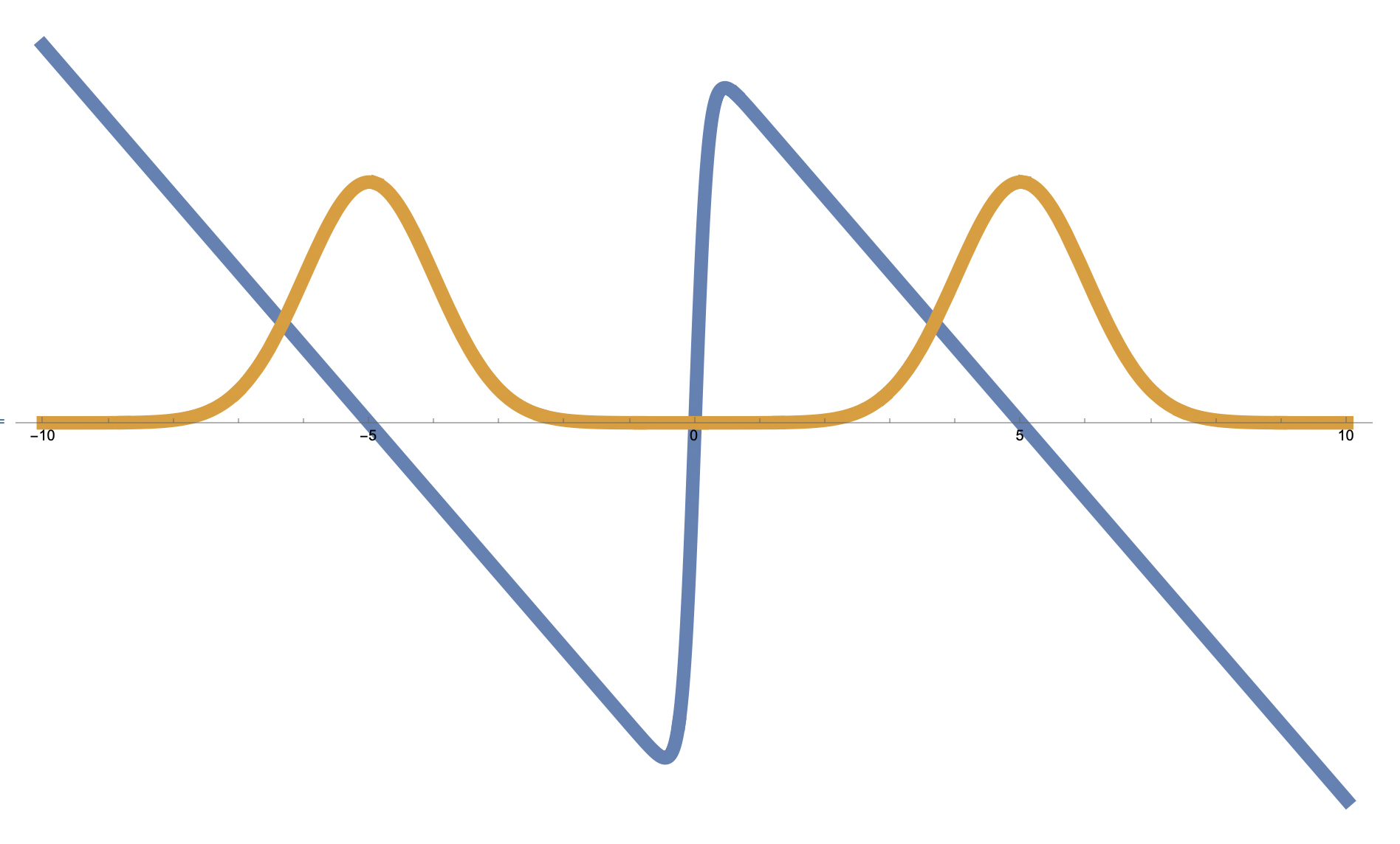
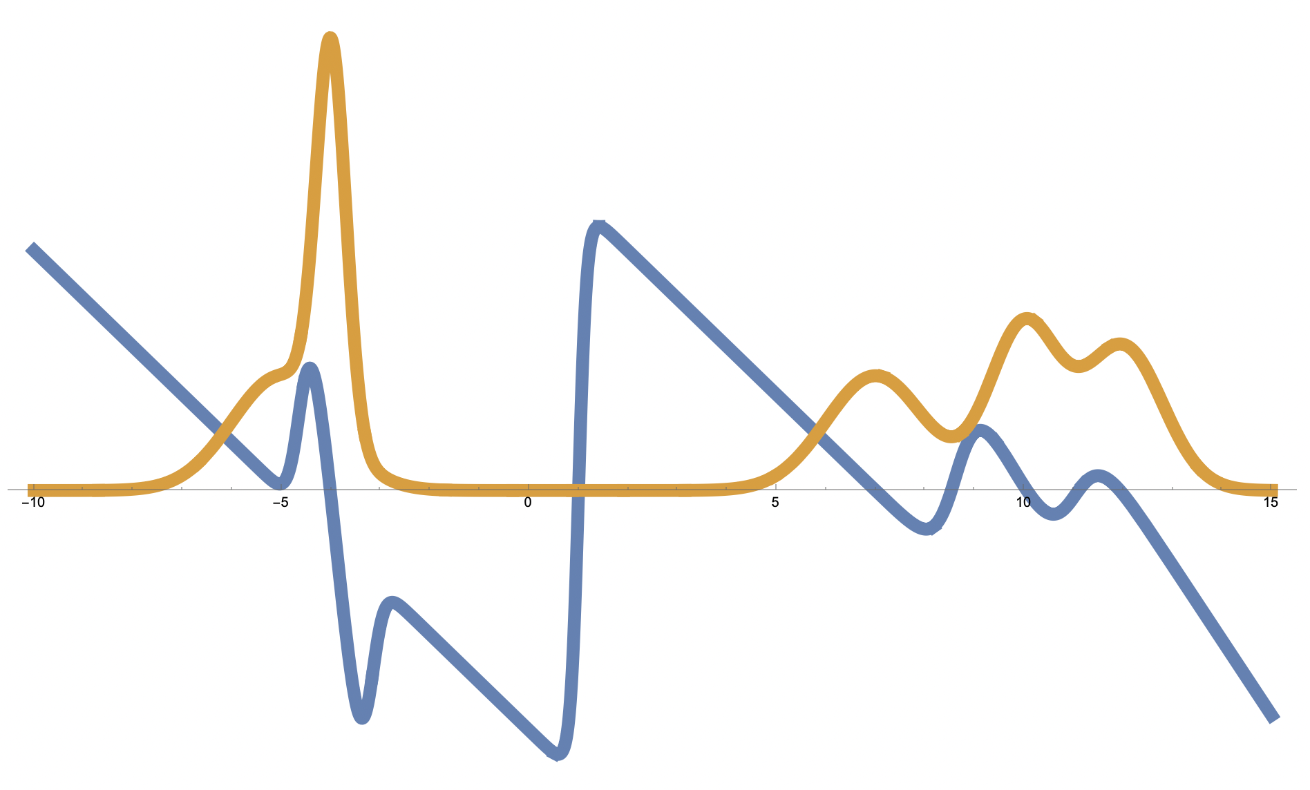
Figure 1: When approximation is hard, clustering is easy. On the left figure, we plot the density (gold) and score function (blue) of mixtures of two standard Gaussians with well-separated means (their distance is $R$). We observe that in that case, the score function is (almost) a piecewise linear function with a large slope, i.e., roughly $R$, close to the origin. In the right image, we have a mixture of $5$ Gaussians with different means and variances that can be split into two clusters: a group of $2$ on the left and $3$ on the right. Again the area where the derivative of the score function (blue) is high, falls in between the two clusters (where the Gaussian density is exponentially small). In both cases, a piecewise polynomial approximation yields the correct degree that scaling with $(\log R)/\varepsilon$ instead of $R/\varepsilon$. Moreover, we expect that it is easy to cluster the points in the corresponding sub-mixtures that have much smaller effective support than the original mixture.

2.3 Approximating the score given a crude partition

As we observed in the previous examples, the main difficulty in providing a polynomial approximation of the score function arises when it involves multiple Gaussians that are far apart. We first make more precise the notion of “crude” clustering that we require.

Definition 2.4 ($(\Delta_{\rm in},\Delta_{\rm out})$-separated partition).

Given a mixture of Gaussians $\mathcal{N}_{1}=\mathcal{N}(\boldsymbol{\mathrm{\mu}}_{1},\boldsymbol{\mathrm{Q}}_{1}),\ldots,\mathcal{N}_{k}=\mathcal{N}(\boldsymbol{\mathrm{\mu}}_{k},\boldsymbol{\mathrm{Q}}_{k})$, we require that the clustering function $\mathsf{c}(\boldsymbol{\mathrm{x}})$ assigns each $\boldsymbol{\mathrm{x}}\in\mathbb{R}^{d}$ to one of $n_{c}$ subsets $U_{1},\ldots,U_{n_{c}}$ of $[k]$ that form a partition of the original $k$ components such that:

1. If $\mathcal{N}_{i},\mathcal{N}_{j}$ belong in different subsets $U_{t}$ and $U_{t^{\prime}}$, they have to be at least $\Delta_{\rm out}=\mathrm{poly}(\tau k\log(1/\varepsilon))$ far in parameter distance, i.e., $D_{p}(\mathcal{N}_{i},\mathcal{N}_{j})=\|\boldsymbol{\mathrm{\mu}}_{i}-\boldsymbol{\mathrm{\mu}}_{j}\|_{2}+\|\boldsymbol{\mathrm{Q}}_{i}-\boldsymbol{\mathrm{Q}}_{j}\|_{F}\geq\Delta_{\rm out}$.

2. If $\mathcal{N}_{i},\mathcal{N}_{j}$ belong in the same subset $U_{t}$, they have to be at most $\Delta_{\rm in}=\mathrm{poly}(\tau k\log(1/\varepsilon))$ far in parameter distance, i.e., $D_{p}(\mathcal{N}_{i},\mathcal{N}_{j})\leq\Delta_{\rm in}$.

3. $\mathsf{c}(\boldsymbol{\mathrm{x}})$ is consistent with the partition $U_{1},\ldots,U_{t}$ with high-probability, i.e., for any $i\in U_{t}$, $\operatorname*{\mathbb{P}}_{\boldsymbol{\mathrm{x}}\sim\mathcal{N}_{i}}[\mathsf{c}(\boldsymbol{\mathrm{x}})\neq t]\leq\varepsilon_{\mathrm{part}}$.

Given the above $(\Delta_{\rm in},\Delta_{\rm out})$-partition, our proof consists of two steps: (i) show that we can reduce the original problem of approximating the score function of the whole mixture to approximating the score function of the sub-mixtures $U_{t}$ and (ii) providing low-degree approximations of the sub-mixture score functions. We describe these steps in the next two paragraphs.

Simplifying the score

As we discussed, the first obstacle in approximating the score function is that it is a function over a domain of radius $\mathrm{poly}(R)$ (inducing a $\mathrm{poly}(R)$ dependency on the degree). Fortunately, there is an additional structure connecting the weights $w_{i}(\boldsymbol{\mathrm{x}})$ and the linear terms $\boldsymbol{\mathrm{g}}_{i}(\boldsymbol{\mathrm{x}})$. We use this structure to prove that when $\boldsymbol{\mathrm{x}}$ is sampled from some component $\mathcal{N}_{i}$ then on expectation over the component $\mathcal{N}_{i}$ we can remove a term in the score function corresponding to a component $\mathcal{N}_{j}$ that is far from $\mathcal{N}_{i}$ without introducing large error, see Lemma 7.3. More precisely, we show that given a partition function $\mathsf{c}(\cdot)$ that satisfies Definition 2.4, for all $\boldsymbol{\mathrm{x}}$ where $\mathsf{c}(\boldsymbol{\mathrm{x}})=t$, we can “simplify” the score function by removing the contribution of all components $\mathcal{N}_{j}$ that do not belong in $U_{t}$.

Given a subset $U_{t}$ of indices of $[k]$, we denote by $\mathcal{M}(U_{t})$ the submixture containing the components $\mathcal{N}_{i}$ for $i\in U_{t}$ and by $\boldsymbol{\mathrm{s}}(\boldsymbol{\mathrm{x}};\mathcal{M}(U_{t}))$ the score function containing only the contribution of components from $U_{t}$, i.e.,

$$\boldsymbol{\mathrm{s}}(\boldsymbol{\mathrm{x}};\mathcal{M}(U_{t}))=-\sum_{i\in U_{t}}\boldsymbol{\mathrm{g}}_{i}(\boldsymbol{\mathrm{x}})\frac{\lambda_{i}\mathcal{N}_{i}(\boldsymbol{\mathrm{x}})}{\sum_{j\in U_{t}}\lambda_{j}\mathcal{N}_{j}(\boldsymbol{\mathrm{x}})}$$

We prove the following proposition showing that, inside each cell $t$ of the partition given by $\mathsf{c}(\cdot)$, we can replace the original score function $\boldsymbol{\mathrm{s}}(\boldsymbol{\mathrm{x}};\mathcal{M})$ by the score function of the sub-mixture $\boldsymbol{\mathrm{s}}(\boldsymbol{\mathrm{x}};\mathcal{M}(U_{t}))$. Each sub-mixture score function corresponding to $U_{t}$ contains components that are all $\Delta_{\rm in}$-close to each other, thus reducing the effective radius of the approximation domain to $\mathrm{poly}(\log R)$.

Proposition 2.5 (Informal – Score Simplification, see Proposition 7.1).

Fix $\varepsilon>0$ and let $\mathcal{M}$ be a $\tau$-well-conditioned mixture of $k$ Gaussian distributions. Moreover, assume that $\mathsf{c}$ satisfies Definition 2.4. Define the following piecewise approximation to the score function $s(\boldsymbol{\mathrm{x}};\mathsf{c}(\cdot))=\sum_{t=1}^{{n_{\rm c}}}s(\boldsymbol{\mathrm{x}};\mathcal{M}(U_{t}))~{}\mathds{1}\{\mathsf{c}(\boldsymbol{\mathrm{x}})=t\}\,.$ It holds that $\operatorname*{\mathbb{E}}_{\boldsymbol{\mathrm{x}}\sim\mathcal{M}}[\|s(\boldsymbol{\mathrm{x}};\mathcal{M})-s(\boldsymbol{\mathrm{x}};\mathsf{c}(\cdot))\|_{2}^{2}]\leq\mathrm{poly}(k\tau R)\sqrt{\varepsilon}.$

Polynomial approximation of the simplified score

Recall from Eq. (4) that the score function for any Gaussian mixture is a sum of the softmax function $w_{i}(\boldsymbol{\mathrm{x}})$ multiplied by a linear function $\boldsymbol{\mathrm{Q}}_{i}^{-1}(\boldsymbol{\mathrm{x}}-\boldsymbol{\mathrm{\mu}}_{i})$. A polynomial approximation of the softmax will provide a polynomial approximation for the simplified score. Note that we want to approximate the simplified score with the degree at most $\mathrm{poly}(k\tau/\varepsilon)$ to obtain runtime of polynomial regression of $O(d^{\mathrm{poly}(k\tau/\varepsilon)})$.

The degree of a polynomial approximation of a function generally depends on the domain of the approximation and smoothness of the function (in terms of the norm of its gradient), see Lemma 8.2. The softmax function is smooth and has a bounded gradient but the input to the softmax is $\{\|\boldsymbol{\mathrm{x}}-\boldsymbol{\mathrm{\mu}}_{i}\|^{2}_{\boldsymbol{\mathrm{Q}}_{i}^{-1}}\}_{i=1}^{|U_{t}|}$ which can be as large as $\mathrm{poly}(d)$ and hence, the degree of the naive polynomial approximation could be $\mathrm{poly}(d/\varepsilon)$.

To overcome this issue, we show that even though each input $\|\boldsymbol{\mathrm{x}}-\boldsymbol{\mathrm{\mu}}_{i}\|_{\boldsymbol{\mathrm{Q}}_{i}^{-1}}^{2}$ is large, there exists a normalization of the softmax for which the inputs to the softmax are $\mathrm{poly}(\tau\Delta_{\rm in})$. More precisely, we normalize the softmax such that $\{\|\boldsymbol{\mathrm{x}}-\boldsymbol{\mathrm{\mu}}_{i}\|^{2}_{\boldsymbol{\mathrm{Q}}_{i}^{-1}}-\|\boldsymbol{\mathrm{x}}-\boldsymbol{\mathrm{\mu}}_{1}\|^{2}_{\boldsymbol{\mathrm{Q}}_{1}^{-1}}-\langle\boldsymbol{\mathrm{Q}}_{1},\boldsymbol{\mathrm{Q}}_{i}^{-1}-\boldsymbol{\mathrm{Q}}_{1}^{-1}\rangle\}_{i=1}^{|U_{t}|}$ are the inputs to the softmax function and show that its norm is $\mathrm{poly}(\tau\Delta_{\rm in})$ with high probability. Therefore, using multivariate Jackson’s theorem (Lemma 8.2), we obtain the polynomial approximation for the softmax function and hence, for the simplified score function.

Lemma 2.6 (Informal - See Lemma 8.6).

Let $\mathcal{M}(U)$ be a $\tau$-well-conditioned mixture of $k$ Gaussian distributions restricted to the subset of components in $U$. Then, there exist a polynomial $p(\boldsymbol{\mathrm{x}};\mathcal{M}(U))$ of degree $\mathrm{poly}(\tau\Delta_{\rm in}/\varepsilon)$ and coefficients bounded in magnitude by $dR\exp(\mathrm{poly}(\tau\Delta_{\rm in}/\varepsilon))$ such that for $\boldsymbol{\mathrm{x}}\sim\mathcal{M}(U)$, with high probability, the polynomial satisfies $\|s(\boldsymbol{\mathrm{x}};\mathcal{M}(U))-p(\boldsymbol{\mathrm{x}};\mathcal{M}(U))\|\leq\varepsilon.$

2.4 Crude clustering via PCA

We now describe our crude clustering algorithm for obtaining the partition satisfying the assumptions of Definition 2.4. Our approach consists of two main steps: (1) approximately recover the span of the means and covariances using PCA on the second and fourth-order moment tensors of the mixture and (2) recover estimates of the parameters by brute forcing over the $k$-dimensional subspace recovered in the first step and using pairwise log-likelihood tests to create the final partition function.

Obtaining estimates of means and covariances

The algorithm operates in two phases. First, we obtain a crude estimate for the subspace spanned by the means, after which we brute-force within this low-dimensional subspace to find points close to each of the means. Second, we use these mean estimates to form an estimator for the subspace spanned by the covariances, after which we can similarly brute-force to find points close to each of the covariances. With roughly $d^{O(k)}$ runtime, we can construct a list of candidate parameters for the means and covariances of the mixture containing crude (in the sense that they can be $\mathrm{poly}(k\tau)$-far) of the target parameters.

Lemma 2.7 (Informal – Recovering crude estimates of the parameters, see Lemma 5.1).

There is an algorithm that returns a list $\mathcal{W}$ such that for every $i\in[k]$, there exists $(\widehat{\boldsymbol{\mathrm{\mu}}}_{i},\widehat{\boldsymbol{\mathrm{Q}}}_{i})\in\mathcal{W}$ for which $\|\boldsymbol{\mathrm{\mu}}_{i}-\widehat{\boldsymbol{\mathrm{\mu}}}_{i}\|^{2}\lesssim\beta/\lambda_{\rm min}$ and $\|\boldsymbol{\mathrm{Q}}_{i}-\widehat{\boldsymbol{\mathrm{Q}}}_{i}\|_{F}\lesssim k^{3/2}\beta/\lambda_{\rm min}+k^{2}\alpha\log R$. Furthermore, $|\mathcal{W}|\leq(R/\sqrt{\beta})^{O(k^{2})}\cdot d^{O(k)}$, and the algorithm runs in time $(R/\sqrt{\beta})^{O(k^{2})}\cdot(\mathrm{poly}(dR/\beta)+d^{O(k)})$ and draws $\mathrm{poly}(dR/\beta)$ samples.

We use PCA on the covariance of the mixture $\boldsymbol{\mathrm{M}}=\operatorname*{\mathbb{E}}_{\boldsymbol{\mathrm{x}}\sim\mathcal{M}}[\boldsymbol{\mathrm{x}}\boldsymbol{\mathrm{x}}^{\intercal}]$ to obtain the subspace spanned by the means. We observe that $\boldsymbol{\mathrm{M}}=\sum_{i=1}^{k}\lambda_{i}\boldsymbol{\mathrm{\mu}}_{i}\boldsymbol{\mathrm{\mu}}_{i}^{\intercal}+\sum_{i=1}^{k}\lambda_{i}\boldsymbol{\mathrm{Q}}_{i}$. The main idea here is to think of $\boldsymbol{\mathrm{M}}$ as approximately low-rank and treat the contribution of the covariances as an error ${\cal E}=\sum_{i=1}^{k}\lambda_{i}\boldsymbol{\mathrm{Q}}_{i}$. Since the covariance matrices $\boldsymbol{\mathrm{Q}}_{i}$ are well-conditioned (i.e., their eigenvalues are not bigger than $\beta$ (see Definition 1.1) we can show that if some $\boldsymbol{\mathrm{\mu}}_{i}$ is larger than $\beta/\lambda_{\rm min}$ then its contribution in $\boldsymbol{\mathrm{M}}$ cannot be “hidden” by the error term ${\cal E}$ and will have a large projection onto the subspace spanned by the top eigenvectors of $\boldsymbol{\mathrm{M}}$. The proof of this claim follows by a standard argument for $k$-SVD and can be found in Section 5.1.

Finding estimates for the covariances is more complicated but similarly relies on recovering the subspace spanned by the low-rank components of the (flattened) fourth-order tensor

$$\boldsymbol{\mathrm{\Psi}}=\operatorname*{\mathbb{E}}_{\boldsymbol{\mathrm{x}}\sim\mathcal{M}}[\mathrm{vec}(\boldsymbol{\mathrm{x}}\boldsymbol{\mathrm{x}}^{\intercal})\mathrm{vec}(\boldsymbol{\mathrm{x}}\boldsymbol{\mathrm{x}}^{\intercal})]\,.$$

The intuition behind our approach is that if the means of the mixture were all sufficiently close to zero, then the top-$k$ singular subspace of the matrix $\boldsymbol{\mathrm{\Psi}}$ can be shown to contain points close to $\mathrm{vec}(\boldsymbol{\mathrm{Q}}_{1}),\ldots,\mathrm{vec}(\boldsymbol{\mathrm{Q}}_{k})$. In general, if the means are arbitrary, then we can use the estimates $\widehat{\boldsymbol{\mathrm{\mu}}}_{1},\ldots,\widehat{\boldsymbol{\mathrm{\mu}}}_{k}$ derived in the previous section to approximately “recenter” the mixture components near zero. Since the means recovered in the previous step were already crude $\mathrm{poly}(k)$ approximations of the true means a careful error analysis must be done so that this recentering does not introduce significantly more error (i.e., depending on the dimension $d$) in the covariance estimates. We refer to Section 5 and Algorithm 3 for more details.

Clustering using the log-likelihood ratios

We now present our main clustering guarantee, which leverages the estimates for the parameters we obtained previously. As those estimates are only crude approximations to the true parameters, we will obtain a commensurately crude clustering.

Our algorithm starts by brute-forcing over mean-based and covariance-based partitions ${\cal S}$ (resp. ${\cal T}$). ${\cal S}$ (resp. ${\cal T}$) partitions the mixture components into groups such that any two components in the same group have means (resp. covariances) that are not far, and any two components from two different groups have means (resp. covariances) that are not close. Their common refinement is a partition ${\cal U}$ satisfying the assumptions of Definition 2.4: any two components in the same group have both means and covariances not too far, and any two components from two different groups either have means not too close or covariances not too close.

By brute-forcing over pairs of partitions of $[k]$ (of which there are at most $k^{2k}$) we may assume we have access to ${\cal S}$ and ${\cal T}$, and thus to ${\cal U}$. Our goal is then to assign to every $\boldsymbol{\mathrm{x}}\in\mathbb{R}^{d}$ an index into the partition ${\cal U}$. For $\boldsymbol{\mathrm{x}}$ which is sampled from the $i$-th component of the mixture which belongs to the $t$-th group in ${\cal U}$, we would like our assignment to be $t$ with high probability. At a high level, the idea is as follows. It is not too hard to determine which group in ${\cal S}$ a given point $\boldsymbol{\mathrm{x}}$ should belong to, simply by checking which mean estimate $\widehat{\boldsymbol{\mathrm{\mu}}}_{i}$ is closest to $\boldsymbol{\mathrm{x}}$ after projecting to the subspace spanned by $\widehat{\boldsymbol{\mathrm{\mu}}}_{1},\ldots,\widehat{\boldsymbol{\mathrm{\mu}}}_{k}$. For each group in ${\cal S}$, we can then effectively restrict our attention to components within that group and focus on clustering them according to their covariances. Roughly speaking, we accomplish this by comparing log-likelihoods of sampling $\boldsymbol{\mathrm{x}}$ under ${\cal N}(\widehat{\boldsymbol{\mathrm{\mu}}}_{1},\widehat{\boldsymbol{\mathrm{Q}}}_{1}),\ldots,{\cal N}(\widehat{\boldsymbol{\mathrm{\mu}}}_{k},\widehat{\boldsymbol{\mathrm{Q}}}_{k})$ and choosing the group in ${\cal T}$ containing the component maximizing log-likelihood. For more details, we refer to Section 6 and to Proposition 6.2 for the formal clustering statement that we prove.

2.5 Avoiding the doubly exponential dependency on $k$

Here we provide some intuition for the origin of the doubly exponential dependence on $k$ which is implicit in existing works on learning mixtures of general Gaussians with the method of moments, and how our technique outlined above avoids this issue. Our starting point is the algorithm of [MV10]; in fact, for this discussion, it will suffice to consider the case of $d=1$ and components of variance 1.

Specialized to this case, in the analysis in [MV10], the authors first proved that if all of the components have means with nonnegligible separation, say $\eta$, from each other, then one can learn the means by brute-forcing over a grid with sufficiently small granularity and finding a setting of parameters in this grid for which the corresponding mixture matches the first $O(k)$ moments with the target mixture to error $\eta^{k}$ (here we ignore constants in the exponent for simplicity).

Now what happens if the minimal separation $\eta$ is arbitrarily small? The authors noted that for means that are particularly close, one can simply “merge them”: they are statistically close to a single component, and in a bounded number of samples one would not be able to tell the difference. Because the number of samples used by the algorithm outlined above is $(1/\eta)^{k}$, this implies that if there is some scale $\eta$ at which there is a gap in the sense that all means are either $\eta^{k}$-close or $\eta$-far apart, then one can learn in the same amount of time/samples as in the $\eta$-separated case.

The last question that remains is how to ensure such a scale exists. The idea is that if one looks at $k^{2}+1$ consecutive windows $\{[\eta^{k^{i}},\eta^{k^{i-1}}]\}_{i=1,\ldots,k^{2}+1}$, by pigeonhole principle there must exist some window such that the separation between any pair of means lies outside this window. At that scale, one can apply the above reasoning to learn the means. This is the origin of the doubly exponential scaling in $k$ that is present in all existing algorithms for learning mixtures of general Gaussians, including the state-of-the-art guarantee of [BDJ⁺22].

It is instructive to contrast this with our approach. The main reason for the doubly exponential dependence in the above windowing argument was that one needed a scale at which the components break up into “gapped clusters” such that the separation within clusters is significantly smaller than the separation across clusters. For this clustering structure to exist, we need to go down potentially to a doubly exponentially small scale. In contrast, in our work, we make do with a very crude clustering for the purposes of our piecewise regression. We simply require that for components from different clusters, their parameter distance is sufficiently large, while for components from the same cluster, their parameter distance is not too large. Crucially, we don’t need to make any assumption about a gap between the intra- versus inter-cluster separations, ensuring we avoid the doubly exponential dependence on $k$.

3 Notations and technical preliminaries

Notation

Throughout the paper, we use either $q$ or $q_{0}$ to denote the data distribution on $\mathbb{R}^{d}$, i.e., the mixture of Gaussians with means $\boldsymbol{\mathrm{\mu}}_{1},\boldsymbol{\mathrm{\mu}}_{2},\ldots,\boldsymbol{\mathrm{\mu}}_{k}$, covariances $\boldsymbol{\mathrm{Q}}_{1},\boldsymbol{\mathrm{Q}}_{2},\ldots,\boldsymbol{\mathrm{Q}}_{k}$, and mixing weights $\lambda_{1},\ldots,\lambda_{k}$ respectively. We will use $\mathcal{N}_{i}$ to denote the distribution for its $i$-th component, i.e. ${\cal N}(\boldsymbol{\mathrm{\mu}}_{i},\boldsymbol{\mathrm{Q}}_{i})$. We use $p$ or $p_{T}$ to denote the learned distribution.

Definition 3.1.

Let $\mathcal{M}=\frac{1}{k}\sum_{i=1}^{k}\mathcal{N}(\boldsymbol{\mathrm{\mu}}_{i},\boldsymbol{\mathrm{Q}}_{i})$ be a $(\alpha,\beta,R)$-well-conditioned Gaussian mixture. We say that a partition of $[k]$ into subsets $S_{1},\ldots,S_{m}$ is $(\Delta_{\rm in},\Delta_{\rm out})$-separated if for all $i,j\in S_{\ell}$ it holds that $\|\boldsymbol{\mathrm{\mu}}_{i}-\boldsymbol{\mathrm{\mu}}_{j}\|+\|\boldsymbol{\mathrm{Q}}_{i}-\boldsymbol{\mathrm{Q}}_{j}\|_{F}\leq\Delta_{\rm in}$ and for all $i\in S_{\ell}$, $j\in S_{\ell^{\prime}}$ for $\ell\neq\ell^{\prime}$ it holds $\|\boldsymbol{\mathrm{\mu}}_{i}-\boldsymbol{\mathrm{\mu}}_{j}\|+\|\boldsymbol{\mathrm{Q}}_{i}-\boldsymbol{\mathrm{Q}}_{j}\|_{F}\geq\Delta_{\rm out}$. We denote by $\mathcal{M}(S_{i})$ the mixture distribution corresponding to the components of $S_{i}$, i.e., $\mathcal{M}(S_{i})=\frac{1}{|S_{i}|}\sum_{j\in S_{i}}\mathcal{N}(\boldsymbol{\mathrm{\mu}}_{j},\boldsymbol{\mathrm{Q}}_{j})$.

Moreover, given a mixture $\mathcal{M}=\sum_{i=1}^{k}\lambda_{i}\mathcal{D}_{i}$ we denote by $\mathcal{M}^{J}$ the joint distribution over tuples $(j,\boldsymbol{\mathrm{x}})$ where $j=i$ with probability $\lambda_{i}$ and, conditional on $j=i$, $\boldsymbol{\mathrm{x}}$ is drawn from $\mathcal{D}_{i}$.

3.1 Concentration inequalities

We will use the following standard concentration inequality for quadratic forms of Gaussian random variables.

Proposition 3.2 (Hanson-Wright).

Suppose $\boldsymbol{\mathrm{A}}\in\mathbb{R}^{d\times d}$ satisfies $\|\boldsymbol{\mathrm{A}}\|^{2}_{F}/\|\boldsymbol{\mathrm{A}}\|^{2}_{\rm op}\geq r$. Then for any $s>0$,

$$\Pr_{\boldsymbol{\mathrm{x}}\sim{\cal N}(0,\boldsymbol{\mathrm{Id}})}[\boldsymbol{\mathrm{x}}^{\intercal}\boldsymbol{\mathrm{A}}\boldsymbol{\mathrm{x}}-\mathrm{tr}(\boldsymbol{\mathrm{A}})>s\|\boldsymbol{\mathrm{A}}\|_{F}] \leq\exp(-\Omega(\min(s\sqrt{r},s^{2}))$$ (5)

$$\Pr_{\boldsymbol{\mathrm{x}}\sim{\cal N}(0,\boldsymbol{\mathrm{Id}})}[\boldsymbol{\mathrm{x}}^{\intercal}\boldsymbol{\mathrm{A}}\boldsymbol{\mathrm{x}}-\mathrm{tr}(\boldsymbol{\mathrm{A}})<-s\|\boldsymbol{\mathrm{A}}\|_{F}] \leq\exp(-\Omega(\min(s\sqrt{r},s^{2}))\,.$$ (6)

4 Learning Gaussian mixtures via a denoising diffusion process

We start by introducing some standard terminology and notation on diffusion models. We will be using the diffusion algorithmic template in a more or less black box manner and therefore we try to keep the presentation short but still self-contained. Throughout the paper, we use either $q$ or $q_{0}$ to denote the data distribution on $\mathbb{R}^{d}$. The two main components in diffusion models are the forward process and the reverse process. The forward process transforms samples from the data distribution into noise, for instance via the Ornstein-Uhlenbeck (OU) process:

$$\mathrm{d}\boldsymbol{\mathrm{x}}_{t}=-\boldsymbol{\mathrm{x}}_{t}\,\mathrm{d}t+\sqrt{2}\,\mathrm{d}\boldsymbol{\mathrm{w}}_{t}\;\;\;\text{with}\;\;\;\boldsymbol{\mathrm{x}}_{0}\sim q_{0}\,,$$

where $(\boldsymbol{\mathrm{w}}_{t})_{t\geq 0}$ is a standard Brownian motion in $\mathbb{R}^{d}$. We use $q_{t}$ to denote the law of the OU process at time $t$. Note that for $\boldsymbol{\mathrm{x}}_{t}\sim q_{t}$,

$$\boldsymbol{\mathrm{x}}_{t}=\exp(-t)\boldsymbol{\mathrm{x}}_{0}+\sqrt{1-\exp(-2t)}\boldsymbol{\mathrm{z}}_{t}\;\;\;\text{with}\;\;\boldsymbol{\mathrm{x}}_{0}\sim q_{0},\;\;\boldsymbol{\mathrm{z}}_{t}\sim\mathcal{N}(0,\boldsymbol{\mathrm{Id}})\,.$$ (7)

The reverse process then transforms noise into samples, thus performing generative modeling. Ideally, this could be achieved by running the following stochastic differential equation for some choice of terminal time $T$:

$$\mathrm{d}\boldsymbol{\mathrm{x}}^{\leftarrow}_{t}=\{\boldsymbol{\mathrm{x}}^{\leftarrow}_{t}+2\nabla_{\boldsymbol{\mathrm{x}}}\ln q_{T-t}(\boldsymbol{\mathrm{x}}^{\leftarrow}_{t})\}\,\mathrm{d}t+\sqrt{2}\,\mathrm{d}\boldsymbol{\mathrm{w}}_{t}\;\;\;\text{with}\;\;\;\boldsymbol{\mathrm{x}}^{\leftarrow}_{0}\sim q_{T}\,,$$ (8)

where now $\boldsymbol{\mathrm{w}}_{t}$ is the reversed Brownian motion. In this reverse process, the iterate $\boldsymbol{\mathrm{w}}^{\leftarrow}_{t}$ is distributed according to $q_{T-t}$ for every $t\in[0,T]$, so that the final iterate $\boldsymbol{\mathrm{x}}^{\leftarrow}_{T}$ is distributed according to the data distribution $q_{0}$. The function $\nabla_{\boldsymbol{\mathrm{x}}}\ln q_{t}$ is called the score function and is required so that we are able to run the reverse SDE and generate samples from the unknown distribution. Ideally, we would like to have access to an approximate oracle $\widehat{\boldsymbol{\mathrm{s}}}(\boldsymbol{\mathrm{x}})$ such that for all $t\in[0,T]$ it is a good approximation to the score function $\nabla_{\boldsymbol{\mathrm{x}}}\log q_{t}(\boldsymbol{\mathrm{x}})$:

$$\operatorname*{\mathbb{E}}_{\boldsymbol{\mathrm{x}}_{t}\sim q_{t}}[\|\nabla_{\boldsymbol{\mathrm{x}}}\ln q_{t}(\boldsymbol{\mathrm{x}}_{t})-\widehat{\boldsymbol{\mathrm{s}}_{t}}(\boldsymbol{\mathrm{x}}_{t})\|^{2}]\leq\epsilon_{\mathrm{score}}\,.$$ (9)

To obtain such a function $\widehat{\boldsymbol{\mathrm{s}}}_{t}(\boldsymbol{\mathrm{x}})$, one would an expressive enough set of candidate functions $\mathcal{G}$ and then try to optimize the score matching loss:

$$\min_{\boldsymbol{\mathrm{g}}_{t}\in\mathcal{G}}\operatorname*{\mathbb{E}}_{\boldsymbol{\mathrm{x}}_{t}\sim q_{t}}[\|\nabla_{\boldsymbol{\mathrm{x}}}\ln q_{t}(\boldsymbol{\mathrm{x}}_{t})-\boldsymbol{\mathrm{g}}_{t}(\boldsymbol{\mathrm{x}})\|^{2}]\leq\epsilon_{\mathrm{score}}\,.$$

However, as the density function of $q_{t}$ is unknown the above minimization problem cannot be solved directly. A standard calculation (see e.g. Appendix A of [CCL⁺23b]) shows that this is equivalent to minimizing the DDPM objective in which one wants to predict the noise $\boldsymbol{\mathrm{z}}_{t}$ from the noisy observation $\boldsymbol{\mathrm{x}}_{t}$, i.e.

$$\min_{\boldsymbol{\mathrm{g}}\in\mathcal{G}}\;\;L_{t}(\boldsymbol{\mathrm{g}}_{t})=\operatorname*{\mathbb{E}}_{\boldsymbol{\mathrm{x}}_{0},\boldsymbol{\mathrm{z}}_{t}}\Bigl{[}\Big{\|}\boldsymbol{\mathrm{g}}_{t}(\boldsymbol{\mathrm{x}}_{t})+\frac{\boldsymbol{\mathrm{z}}_{t}}{\sqrt{1-\exp(-2t)}}\Big{\|}^{2}\Bigr{]}\,.$$ (10)

In this work we focus specifically on the optimization problem (10) and show that it can be solved efficiently when the underlying target density $q_{0}$ is a mixture of $k$ Gaussian distributions.

Input: Score estimation error $\epsilon_{\mathrm{score}}$, confidence $\delta$, sequence of time steps $t_{0},t_{1},\ldots,t_{N}$

Output: A sample $\boldsymbol{\mathrm{y}}_{N}\in\mathbb{R}^{d}$

1

2 for $\ell\in\{0,\ldots,N-1\}$ do

3       $\widehat{\boldsymbol{\mathrm{s}}}(\cdot,T-t_{\ell})\leftarrow\textsc{LearnScore}(t_{\ell},\epsilon_{\mathrm{score}},\delta)$ $\triangleright$ Learn the score function at all time steps

4      

5 end for

6

7for $\ell\in\{0,\ldots,N-1\}$ do

8       Set $\rho_{\ell}=e^{(t_{\ell+1}-t_{\ell})/2}$

9       Sample $\boldsymbol{\mathrm{z}}_{\ell}\sim\mathcal{N}(\boldsymbol{\mathrm{0}},\boldsymbol{\mathrm{Id}})$

10       $\boldsymbol{\mathrm{y}}_{\ell+1}\leftarrow~{}\rho_{\ell}~{}\boldsymbol{\mathrm{y}}_{\ell}+2(\rho_{\ell}-1)~{}\widehat{\boldsymbol{\mathrm{s}}}(\boldsymbol{\mathrm{y}}_{\ell},T-t_{\ell})+\sqrt{\rho_{\ell}^{2}-1}~{}\boldsymbol{\mathrm{z}}_{\ell}$   $\triangleright$ Run the (discretized) reverse SDE

11 end for

12

return $\boldsymbol{\mathrm{y}}_{N}$

Algorithm 1 GenerateSample

We are now ready to present and prove our main result: an efficient algorithm for learning well-conditioned GMMs.

Theorem 4.1 (Efficient Sampler for GMMs).

Fix $\varepsilon,\delta\in(0,1)$ and let $\mathcal{M}$ be an $(\alpha,\beta,R)$-well-conditioned mixture of $k$ Gaussians. Let $\tau=(\beta/\alpha)\,\log R$, $\varepsilon_{\text{score}}=\varepsilon/\log(R/(\alpha\varepsilon))$, $\delta=\alpha\varepsilon/R$, and let time sequence $t_{1},\ldots,t_{N}$ be as defined in Lemma 4.2. Then with probability at least $1-\delta_{\text{f}}$, Algorithm 1 draws $M=d^{\mathrm{poly}(k\tau/(\lambda_{\rm min}\varepsilon))}\log\frac{1}{\delta_{\text{f}}}$ samples from $\mathcal{M}$, runs in sample-polynomial time, and generates a sample $\boldsymbol{\mathrm{y}}_{N}$ whose distribution is $\varepsilon$-close in total variation to $\mathcal{M}$.

Proof.

We are going to use the following result on the convergence of the discretized reverse SDE with the score approximation that we use in Algorithm 1.

Lemma 4.2 (Convergence given approximate scores, [BDBDD23]).

Fix some $\delta\in(0,1)$, $T\geq 1$ and let $N$ be some even integer larger than $\log(1/\delta)$ and let $\kappa>0$ be larger than a sufficiently large constant multiple of $(T+\log(1/\delta))/N$. Set $t_{0}=0$, $t_{N/2}=T-1$, $t_{N}=T-\delta$. Moreover, set $t_{1},\ldots,t_{N/2-1}$ equally spaced on $[0,T-1]$, i.e., $t_{\ell+1}-t_{\ell}=\kappa>0$ for all $\ell\in\{0,\ldots,N/2-1\}$ and $T-t_{N/2+1},\ldots T-t_{N-1}$ exponentially decaying, i.e., $t_{N/2+\ell+1}-t_{N/2+\ell}=\kappa/(1+\kappa)^{\ell}$ for all $\ell\in\{0,\ldots,N/2-2\}$ and $\gamma_{\ell}\leq\kappa\min(1,T-t_{\ell})$. Assume that the data distribution and the score function satisfy the following assumptions.

1. $\sum_{\ell=0}^{N-1}\gamma_{\ell}\operatorname*{\mathbb{E}}_{\boldsymbol{\mathrm{x}}\sim q_{t_{\ell}}}[\|\nabla\log q_{T-t_{\ell}}(\boldsymbol{\mathrm{x}})-\widehat{\boldsymbol{\mathrm{s}}}(\boldsymbol{\mathrm{x}},T-t_{\ell})\|_{2}^{2}]\leq\epsilon_{\mathrm{score}}^{2}$.

2. The target distribution $q_{0}$ on $\mathbb{R}^{d}$ has finite second moment.

For any $t\in[0,T]$ denote by $q_{t}$ the distribution of $\exp(-t)\boldsymbol{\mathrm{x}}_{0}+\sqrt{1-\exp(-2t)}\boldsymbol{\mathrm{z}}_{t}$, where $\boldsymbol{\mathrm{x}}_{0}\sim q_{0}$ and $\boldsymbol{\mathrm{z}}_{t}\sim\mathcal{N}(\boldsymbol{\mathrm{0}},\boldsymbol{\mathrm{Id}})$ and denote by $p_{t_{N}}$ the distribution of the output $\boldsymbol{\mathrm{y}}_{N}$ of Algorithm 1. It holds that

$$\mathrm{KL}(q_{\delta}\|p_{t_{N}})\lesssim\epsilon_{\mathrm{score}}^{2}+\kappa^{2}dN+\kappa dT+\mathrm{KL}(q_{T}\|\mathcal{N}(\boldsymbol{\mathrm{0}},\boldsymbol{\mathrm{Id}}))\,.$$

We first show that the guarantee of Lemma 4.2 yields a total variation bound between $p_{t_{N}}$ and the target Gaussian mixture $\mathcal{M}$. By Pinsker’s inequality, we obtain that $\mathrm{TV}(p_{t_{N}},q_{\delta})\lesssim\sqrt{\mathrm{KL}(q_{\delta}\|p_{t_{N}})}$. Moreover, by a triangle inequality, we obtain that $\mathrm{TV}(q_{0},p_{t_{N}})\leq\mathrm{TV}(p_{t_{N}},q_{\delta})+\mathrm{TV}(q_{\delta},q_{0})$. Therefore, we have to control $\mathrm{TV}(q_{0},q_{\delta})$. Using again Pinsker’s inequality we obtain that $\mathrm{TV}(q_{0},q_{\delta})\lesssim\sqrt{\mathrm{KL}(q_{0}\|q_{\delta})}$. To control the Kullback-Leibler divergence between the target $q_{0}$ that corresponds to the well-conditioned mixture and $q_{\delta}$. We observe that $q_{\delta}$ is also a Gaussian mixture with parameters $\widehat{\boldsymbol{\mathrm{\mu}}}_{i}=\boldsymbol{\mathrm{\mu}}_{i}\exp(-\delta)$ and $\widehat{\boldsymbol{\mathrm{Q}}}=\boldsymbol{\mathrm{Q}}_{i}e^{-2\delta}+(1-e^{-2\delta})~{}\boldsymbol{\mathrm{Id}}$. We denote this mixture by $\mathcal{M}_{\delta}$ Since $\mathrm{KL}$ is convex we obtain that

$$\mathrm{KL}(q_{\delta}\|q_{0})\leq\sum_{i=1}^{k}\lambda_{i}\mathrm{KL}(\mathcal{N}(\boldsymbol{\mathrm{\mu}}_{i},\boldsymbol{\mathrm{Q}}_{i})\|\mathcal{N}(\widehat{\boldsymbol{\mathrm{\mu}}}_{i},\widehat{\boldsymbol{\mathrm{Q}}}_{i}))\leq\max_{i=1}^{k}\mathrm{KL}(\mathcal{N}(\boldsymbol{\mathrm{\mu}}_{i},\boldsymbol{\mathrm{Q}}_{i})\|\mathcal{N}(\widehat{\boldsymbol{\mathrm{\mu}}}_{i},\widehat{\boldsymbol{\mathrm{Q}}}_{i}))\,.$$

We can now use the following standard bound for the Kullback-Leibler distance between two Normal distributions $\mathrm{KL}(\mathcal{N}(\boldsymbol{\mathrm{\mu}}_{1},\boldsymbol{\mathrm{Q}}_{1})\|\mathcal{N}(\boldsymbol{\mathrm{\mu}}_{2},\boldsymbol{\mathrm{Q}}_{2}))\lesssim\|\boldsymbol{\mathrm{Id}}-\boldsymbol{\mathrm{Q}}_{2}^{-1/2}\boldsymbol{\mathrm{Q}}_{1}\boldsymbol{\mathrm{Q}}_{2}^{-1/2}\|_{F}^{2}+\|\boldsymbol{\mathrm{Q}}_{2}^{-1/2}(\boldsymbol{\mathrm{\mu}}_{1}-\boldsymbol{\mathrm{\mu}}_{2})\|_{2}^{2}$. We have that

$$\|\boldsymbol{\mathrm{Q}}_{i}^{-1/2}(\boldsymbol{\mathrm{\mu}}_{i}-\boldsymbol{\mathrm{\mu}}_{i}e^{-\delta})\|_{2}^{2}\leq\frac{R^{2}}{\alpha}(1-e^{-\delta})^{2}\leq\frac{R^{2}}{\alpha}~{}\delta^{2}\,,$$

where the last inequality follows by the fact that $\alpha\boldsymbol{\mathrm{Id}}\preceq\boldsymbol{\mathrm{Q}}_{i}$ and the fact that $\|\boldsymbol{\mathrm{\mu}}_{i}\|_{2}\leq R$ and the inequality $e^{x}\geq x+1$. Moreover, if $s_{1},\ldots s_{d}$ are the eigenvalues of $\boldsymbol{\mathrm{Q}}_{1}$, we have that

$$\|\boldsymbol{\mathrm{Id}}-\boldsymbol{\mathrm{Q}}_{2}^{-1/2}\boldsymbol{\mathrm{Q}}_{1}\boldsymbol{\mathrm{Q}}_{2}^{-1/2}\|_{F}^{2}=\sum_{i=1}^{d}\Big{(}1-\frac{s_{i}e^{-2\delta}+(1-e^{-2\delta})}{s_{i}}\Big{)}^{2}=(1-e^{-2\delta})^{2}\sum_{i=1}^{d}\Big{(}\frac{1-s_{i}}{s_{i}}\Big{)}^{2}\lesssim\frac{\delta^{2}}{\alpha^{2}}R^{2}\,,$$

where the last inequality follows by the assumption that $\|\boldsymbol{\mathrm{Q}}_{i}-\boldsymbol{\mathrm{Id}}\|_{F}^{2}\lesssim R$ and the fact that $s_{i}\geq\alpha$ for all $i$. Putting the above together, we obtain that $\mathrm{TV}(p_{t_{N}},\mathcal{M})\lesssim\sqrt{\mathrm{KL}(q_{\delta}\|p_{t_{N}})}+\delta R/\alpha$.

Similarly, we have to control the convergence error of the forward OU process $\mathrm{KL}(q_{T}\|\mathcal{N}(\boldsymbol{\mathrm{0}},\boldsymbol{\mathrm{Id}}))$. Similarly to the above argument, by the convexity of the Kullback-Leibler, we obtain that it suffices to control the KL divergence between any component of the mixture and the standard normal $\mathcal{N}(\boldsymbol{\mathrm{0}},\boldsymbol{\mathrm{Id}})$. Using the same bound for the KL divergence as above, we have that

$$\mathrm{KL}(q_{T}\|\mathcal{N}(\boldsymbol{\mathrm{0}},\boldsymbol{\mathrm{Id}})\leq\max_{i=1}^{k}(e^{-2T}\|\boldsymbol{\mathrm{\mu}}_{i}\|_{2}^{2}+e^{-4T}\|\boldsymbol{\mathrm{Q}}_{i}-\boldsymbol{\mathrm{Id}}\|_{F}^{2})\lesssim e^{-2T}R^{2}\,.$$

To make the forward process converge to an $\varepsilon$-approximate Gaussian, we take $T=\log(R/\varepsilon)$. We choose $\varepsilon_{\text{score}}=\varepsilon/\log(R/(\alpha\varepsilon))$ and $\delta=\alpha\varepsilon/R$. Additionally, we have $\gamma_{\ell}\leq\kappa$ for all $\ell$. Therefore, we have

$$\sum_{\ell=0}^{N-1}\gamma_{\ell}\operatorname*{\mathbb{E}}_{\boldsymbol{\mathrm{x}}\sim q_{t_{\ell}}}[\|\nabla\log q_{T-t_{\ell}}(\boldsymbol{\mathrm{x}})-\widehat{\boldsymbol{\mathrm{s}}}(\boldsymbol{\mathrm{x}},T-t_{\ell})\|_{2}^{2}]\leq\varepsilon\;.$$

The above choice also yields $\kappa^{2}dN\lesssim(\log^{2}(R/\alpha\varepsilon)d)/N$ and $\kappa dT\lesssim(\log^{2}(R/\alpha\varepsilon)d)/N$. Choosing $N=(\log^{2}(R/\alpha\varepsilon)d)/\varepsilon$ and combining all the terms in Lemma 4.2, we obtain that $\mathrm{TV}(p_{t_{N}},\mathcal{M})\leq\varepsilon$. We obtain sample complexity and runtime of the algorithm by putting $\varepsilon_{\text{score}}=\varepsilon/\log(R/(\alpha\varepsilon))$ and failure probability $\delta_{f}=\delta/N$ in Proposition 8.10.

∎

5 Obtaining crude estimates for the parameters

In this section, we prove the next lemma showing that we can construct a list of candidates for the unknown parameters of the mixture, containing “crude” approximation to the true target parameters.

Lemma 5.1.

There is an algorithm CrudeEstimate($q$) which returns a list $\mathcal{W}$ such that for every $i\in[k]$, there exists $(\widehat{\boldsymbol{\mathrm{\mu}}}_{i},\widehat{\boldsymbol{\mathrm{Q}}}_{i})\in\mathcal{W}$ for which $\|\boldsymbol{\mathrm{\mu}}_{i}-\widehat{\boldsymbol{\mathrm{\mu}}}_{i}\|^{2}\lesssim\beta/\lambda_{\rm min}$ and $\|\boldsymbol{\mathrm{Q}}_{i}-\widehat{\boldsymbol{\mathrm{Q}}}_{i}\|_{F}\lesssim k^{3/2}\beta/\lambda_{\rm min}+k^{2}\alpha\log R$. Furthermore, $|\mathcal{W}|\leq(R/\sqrt{\beta})^{O(k^{2})}\cdot d^{O(k)}$, and the algorithm runs in time $(R/\sqrt{\beta})^{O(k^{2})}\cdot(\mathrm{poly}(d,1/\beta)+d^{O(k)})$ and draws $\mathrm{poly}(dR/\beta)$ samples.

The algorithm operates in two phases. First, we obtain a crude estimate for the subspace spanned by the means, after which we brute-force within this subspace to find points close to each of the means. Second, we use these mean estimates to form an estimator for the subspace spanned by the covariances, after which we can similarly brute-force to find points close to each of the covariances.

5.1 Estimating the means

This phase is straightforward: we simply take the top-$k$ singular subspace of the empirical second moment matrix (see Algorithm 2 below).

Lemma 5.2.

There is an algorithm CrudeEstimateMeans($q$) which returns a list $\mathcal{W}$ such that for each $i\in[k]$, there exists $\widehat{\boldsymbol{\mathrm{\mu}}}_{i}\in\mathcal{W}$ for which $\|\boldsymbol{\mathrm{\mu}}_{i}-\widehat{\boldsymbol{\mathrm{\mu}}}_{i}\|^{2}\lesssim\beta/\lambda_{\rm min}$. Fuurthermore, $|\mathcal{W}|\leq(R/\sqrt{\beta})^{O(k)}$, and the algorithm runs in time $\mathrm{poly}(dR/\beta)+(R/\sqrt{\beta})^{O(k)}$ and draws $\mathrm{poly}(dR/\beta)$ samples.

Input: Sample access to $q$

Output: List $\mathcal{W}$ containing approximations to $\boldsymbol{\mathrm{\mu}}_{1},\ldots,\boldsymbol{\mathrm{\mu}}_{k}$

1 Draw samples $\boldsymbol{\mathrm{x}}_{1},\ldots,\boldsymbol{\mathrm{x}}_{N}$ from $q$ for $N\leftarrow\mathrm{poly}(dR/\beta)$

2 $\widehat{\boldsymbol{\mathrm{M}}}\leftarrow\frac{1}{N}\sum_{i}\boldsymbol{\mathrm{x}}_{i}\boldsymbol{\mathrm{x}}_{i}^{\intercal}$

3 $\widehat{V}\leftarrow$ top-$k$ singular subspace of $\widehat{\boldsymbol{\mathrm{M}}}$

4 $\mathcal{W}\leftarrow$ a $\beta^{1/2}$-net over vectors in $\widehat{V}$ with $L_{2}$ norm at most $2R$

return $\mathcal{W}$

Algorithm 2 CrudeEstimateMeans($q$)

The analysis (as well as subsequent parts of our proof) uses the following standard bound for $k$-SVD:

Lemma 5.3.

Let $\boldsymbol{\mathrm{A}}=\sum^{k}_{i=1}\boldsymbol{\mathrm{v}}_{i}\boldsymbol{\mathrm{v}}_{i}^{\intercal}+\boldsymbol{\mathrm{E}}$ for $\|\boldsymbol{\mathrm{E}}\|_{\rm op}\leq\epsilon$. The top-$k$ singular subspace of $\boldsymbol{\mathrm{A}}$ contains vectors $\widehat{\boldsymbol{\mathrm{v}}}_{1},\ldots,\widehat{\boldsymbol{\mathrm{v}}}_{k}$ for which $\|\boldsymbol{\mathrm{v}}_{i}-\widehat{\boldsymbol{\mathrm{v}}}_{i}\|^{2}\leq 2\epsilon$ for all $i\in[k]$.

Proof.

Define $\boldsymbol{\mathrm{A}}^{*}\coloneqq\sum^{k}_{i=1}\boldsymbol{\mathrm{v}}_{i}\boldsymbol{\mathrm{v}}_{i}^{\intercal}$. Let $\Pi^{\perp}$ denote the projector to the orthogonal complement of the top-$k$ singular subspace of $\boldsymbol{\mathrm{A}}$, and define $\boldsymbol{\mathrm{r}}_{i}\coloneqq\Pi^{\perp}\boldsymbol{\mathrm{v}}_{i}$. Then

$$\boldsymbol{\mathrm{r}}_{i}^{\intercal}\boldsymbol{\mathrm{A}}^{*}\boldsymbol{\mathrm{r}}_{i}=\sigma_{k+1}(\boldsymbol{\mathrm{A}})\cdot\|\boldsymbol{\mathrm{r}}_{i}\|^{2}-\boldsymbol{\mathrm{r}}_{i}^{\intercal}\boldsymbol{\mathrm{E}}\boldsymbol{\mathrm{r}}_{i}\leq 2\epsilon\|\boldsymbol{\mathrm{r}}_{i}\|^{2}\,,$$

where in the last step we used Weyl’s inequality to bound $\sigma_{k+1}(\boldsymbol{\mathrm{A}})$.

On the other hand,

$$\boldsymbol{\mathrm{r}}_{i}^{\intercal}\boldsymbol{\mathrm{A}}^{*}\boldsymbol{\mathrm{r}}_{i}=\sum_{j}\langle\boldsymbol{\mathrm{r}}_{i},\boldsymbol{\mathrm{v}}_{j}\rangle^{2}\geq\langle\boldsymbol{\mathrm{r}}_{i},\boldsymbol{\mathrm{v}}_{i}\rangle^{2}=\|\boldsymbol{\mathrm{r}}_{i}\|^{4}\,,$$

so we conclude that $\|\boldsymbol{\mathrm{r}}_{i}\|^{2}\leq 2\epsilon$. If we define $\widehat{\boldsymbol{\mathrm{v}}}_{i}=\Pi\boldsymbol{\mathrm{v}}_{i}$, where $\Pi$ is the projector to the top-$k$ singular subspace of $\boldsymbol{\mathrm{A}}$, then $\|\widehat{\boldsymbol{\mathrm{v}}}_{i}-\boldsymbol{\mathrm{v}}_{i}\|^{2}=\|\boldsymbol{\mathrm{r}}_{i}\|^{2}\leq 2\epsilon$ as claimed. ∎

We now show that the empirical second moment matrix can be used to extract a rough approximation to the span of the means:

Lemma 5.4.

For $\boldsymbol{\mathrm{x}}\sim\mathcal{M}$, let $\boldsymbol{\mathrm{M}}\coloneqq\operatorname*{\mathbb{E}}[\boldsymbol{\mathrm{x}}\boldsymbol{\mathrm{x}}^{\intercal}]$. Given $\widehat{\boldsymbol{\mathrm{M}}}$ for which $\|\boldsymbol{\mathrm{M}}-\widehat{\boldsymbol{\mathrm{M}}}\|_{\rm op}\lesssim\beta$, let $\widehat{V}$ denote the top-$k$ singular subspace of $\widehat{\boldsymbol{\mathrm{M}}}$. Then for every $i\in[k]$, there exists $\widehat{\boldsymbol{\mathrm{\mu}}}_{i}\in\widehat{V}$ for which $\|\widehat{\boldsymbol{\mathrm{\mu}}}_{i}-\boldsymbol{\mathrm{\mu}}_{i}\|^{2}\lesssim\beta/\lambda_{\rm min}$.

Proof.

Define ${\cal E}=\sum_{i}\lambda_{i}\boldsymbol{\mathrm{Q}}_{i}$ and $\boldsymbol{\mathrm{M}}^{*}\coloneqq\sum_{i}\lambda_{i}\mu_{i}\mu_{i}^{\intercal}$. We have that

$$\boldsymbol{\mathrm{M}}=\boldsymbol{\mathrm{M}}^{*}+{\cal E}\,,$$

and $\|{\cal E}\|_{\rm op}\lesssim\beta$.

By Lemma 5.3, where we take $\boldsymbol{\mathrm{A}}$ and $\boldsymbol{\mathrm{E}}$ therein to be $\widehat{\boldsymbol{\mathrm{M}}}$ and ${\cal E}+\widehat{\boldsymbol{\mathrm{M}}}-\boldsymbol{\mathrm{M}}$, we find that $\widehat{V}$ contains vectors $\boldsymbol{\mathrm{\mu}}^{\prime}_{1},\ldots,\boldsymbol{\mathrm{\mu}}^{\prime}_{k}$ for which $\|\boldsymbol{\mathrm{\mu}}^{\prime}_{i}-\sqrt{\lambda}_{i}\boldsymbol{\mathrm{\mu}}_{i}\|^{2}\lesssim\beta$. So if we take $\widehat{\boldsymbol{\mathrm{\mu}}}_{i}=\boldsymbol{\mathrm{\mu}}^{\prime}_{i}/\sqrt{\lambda_{i}}$, the claimed bound follows. ∎

Proof of Lemma 5.2.

By standard matrix concentration (see, e.g., [Ver18]) with $N=\mathrm{poly}(dR/\beta)$ samples (as set in Algorithm 2) we have that the matrix $\widehat{\boldsymbol{\mathrm{M}}}$ constructed therein satisfies $\|\widehat{\boldsymbol{\mathrm{M}}}-\boldsymbol{\mathrm{M}}\|_{\rm op}\leq\beta$, where $\boldsymbol{\mathrm{M}}\coloneqq\operatorname*{\mathbb{E}}_{\mathcal{M}}[\boldsymbol{\mathrm{x}}\boldsymbol{\mathrm{x}}^{\intercal}]=\sum_{i}\lambda_{i}\boldsymbol{\mathrm{\mu}}_{i}\boldsymbol{\mathrm{\mu}}_{i}^{\intercal}+\sum_{i}\lambda_{i}\boldsymbol{\mathrm{Q}}_{i}$. We have $\|\widehat{\boldsymbol{\mathrm{M}}}-\sum_{i}\lambda_{i}\boldsymbol{\mathrm{\mu}}_{i}\boldsymbol{\mathrm{\mu}}_{i}^{\intercal}\|_{\rm op}\leq 2\beta$, so by Lemma 5.4, the $\beta$-net constructed in Algorithm 2 contains points which are $O(\beta/\lambda_{\rm min})$-close to each of the means $\boldsymbol{\mathrm{\mu}}_{i}$ as claimed. ∎

5.2 Estimating the covariances

Next, we show how to recover a rough approximation to the span of the covariance matrices and, as a consequence, produce a net containing rough approximations to each of the covariance matrices. The algorithm is summarized in Algorithm 3.

Lemma 5.5.

Suppose $\widehat{\boldsymbol{\mathrm{\mu}}}_{1},\ldots,\widehat{\boldsymbol{\mathrm{\mu}}}_{k}\in\mathbb{R}^{d}$ satisfy $\|\boldsymbol{\mathrm{\mu}}_{i}-\widehat{\boldsymbol{\mathrm{\mu}}}_{i}\|^{2}\leq\upsilon_{\rm mean}$ for all $i\in[k]$. Then there is an algorithm CrudeEstimateCovariances($q,\{\widehat{\boldsymbol{\mathrm{\mu}}}_{i}\}$) which returns a list $\mathcal{W}$ such that for each $i\in[k]$, there exists $\widehat{\boldsymbol{\mathrm{Q}}}_{i}\in\mathcal{W}$ for which $\|\boldsymbol{\mathrm{Q}}_{i}-\widehat{\boldsymbol{\mathrm{Q}}}_{i}\|_{F}\lesssim\beta^{1/2}\upsilon_{\rm mean}^{1/2}+k^{3/2}\upsilon_{\rm mean}+k^{5/2}\beta+k^{2}\alpha\log R$. Furthermore $|\mathcal{W}|\leq d^{O(k)}$, and the algorithm runs in time $\mathrm{poly}(dR/\beta)+d^{O(k)}$ and draws $\mathrm{poly}(dR/\beta)$ samples.

The intuition behind our approach is that if the means of the mixture were all sufficiently close to zero, then the top-$k$ singular subspace of the matrix $\operatorname*{\mathbb{E}}[\mathrm{vec}(\boldsymbol{\mathrm{x}}\boldsymbol{\mathrm{x}}^{\intercal})\mathrm{vec}(\boldsymbol{\mathrm{x}}\boldsymbol{\mathrm{x}}^{\intercal})^{\intercal}]$ can be shown to contain points close to $\mathrm{vec}(\boldsymbol{\mathrm{Q}}_{1}),\ldots,\mathrm{vec}(\boldsymbol{\mathrm{Q}}_{k})$. In general, if the means are arbitrary, then we can use the estimates $\widehat{\boldsymbol{\mathrm{\mu}}}_{1},\ldots,\widehat{\boldsymbol{\mathrm{\mu}}}_{k}$ derived in the previous section to approximately “recenter” the mixture components near zero. We now make this intuition precise.

Proof preliminaries.

Define

$$\widehat{\boldsymbol{\mathrm{\Pi}}}\coloneqq\mathrm{span}(\widehat{\boldsymbol{\mathrm{\mu}}}_{1},\ldots,\widehat{\boldsymbol{\mathrm{\mu}}}_{k})\ \ \ \text{and}\ \ \ \widehat{\boldsymbol{\mathrm{\Pi}}}^{\perp}\coloneqq\boldsymbol{\mathrm{Id}}-\widehat{\boldsymbol{\mathrm{\Pi}}}\,.$$

Let $\boldsymbol{\mathrm{\mu}}^{\parallel}_{i}\coloneqq\widehat{\boldsymbol{\mathrm{\Pi}}}\boldsymbol{\mathrm{\mu}}_{i}$ and $\boldsymbol{\mathrm{\mu}}^{\perp}_{i}\coloneqq\widehat{\boldsymbol{\mathrm{\Pi}}}^{\perp}\boldsymbol{\mathrm{\mu}}_{i}$. Note that

$$\|\boldsymbol{\mathrm{\mu}}^{\perp}_{i}\|^{2}=\|\widehat{\boldsymbol{\mathrm{\Pi}}}^{\perp}(\boldsymbol{\mathrm{\mu}}_{i}-\widehat{\boldsymbol{\mathrm{\mu}}}_{i})\|^{2}\leq\upsilon_{\rm mean}\,.$$

Also define

$$\boldsymbol{\mathrm{\zeta}}_{i}\coloneqq\boldsymbol{\mathrm{\mu}}^{\parallel}_{i}-\widehat{\boldsymbol{\mathrm{\mu}}}_{i}$$

and note that

$$\|\boldsymbol{\mathrm{\zeta}}_{i}\|^{2}=\|\widehat{\boldsymbol{\mathrm{\Pi}}}(\boldsymbol{\mathrm{\mu}}_{i}-\widehat{\boldsymbol{\mathrm{\mu}}}_{i})\|^{2}\lesssim\upsilon_{\rm mean}\,.$$

Define $\Delta\geq 1$ by

$$\Delta\coloneqq C(\sqrt{\upsilon_{\rm mean}}+\sqrt{k\beta}+k^{1/4}\sqrt{\alpha\log R})$$ (11)

for sufficiently large absolute constant $C>0$. Given $i\in[k]$, define

$$S_{\rm far}[i]\coloneqq\{j\in[k]:\|\boldsymbol{\mathrm{\mu}}_{i}-\boldsymbol{\mathrm{\mu}}_{j}\|\geq\Delta\}\ \ \ \text{and}\ \ \ S_{\rm close}[i]\coloneqq\{j\in[k]:\|\boldsymbol{\mathrm{\mu}}_{i}-\boldsymbol{\mathrm{\mu}}_{j}\|\leq\Delta\}\,.$$

The algorithm we give in this section (Algorithm 3) does not require knowledge of $S_{\rm far}[i],S_{\rm close}[i]$; these sets are only defined here for the purpose of analysis.

To approximately “recenter” the mixture components around zero, we will subtract from each sample the mean estimate which is closest to it in the subspace given by $\widehat{\boldsymbol{\mathrm{\Pi}}}$. Formally, given $\boldsymbol{\mathrm{x}}\sim\mathbb{R}^{d}$, define $\widehat{\boldsymbol{\mathrm{\mu}}}(\boldsymbol{\mathrm{x}})$ by

$$\widehat{\boldsymbol{\mathrm{\mu}}}(\boldsymbol{\mathrm{x}})\coloneqq\widehat{\boldsymbol{\mathrm{\mu}}}_{i}\ \ \ \text{for}\ \ \ i=\operatorname*{argmin}_{j\in[k]}\|\widehat{\boldsymbol{\mathrm{\mu}}}_{j}-\widehat{\boldsymbol{\mathrm{\Pi}}}\boldsymbol{\mathrm{x}}\|\,.$$ (12)

For every $i\in[k]$, define

$$\mathcal{K}_{i}\coloneqq\{\boldsymbol{\mathrm{x}}\in\mathbb{R}^{d}:\widehat{\boldsymbol{\mathrm{\mu}}}(\boldsymbol{\mathrm{x}})=\widehat{\boldsymbol{\mathrm{\mu}}}_{i}\}\,,$$

i.e. the set of points which are closest to $\widehat{\boldsymbol{\mathrm{\mu}}}_{i}$ in the subspace given by $\widehat{\boldsymbol{\mathrm{\Pi}}}$.

Finally, given $\boldsymbol{\mathrm{z}}\in\mathbb{R}^{d}$, define

$$\boldsymbol{\mathrm{\Psi}}_{00}(\boldsymbol{\mathrm{z}})\coloneqq\mathrm{vec}(\widehat{\boldsymbol{\mathrm{\Pi}}}\boldsymbol{\mathrm{z}}\boldsymbol{\mathrm{z}}^{\intercal}\widehat{\boldsymbol{\mathrm{\Pi}}})\mathrm{vec}(\widehat{\boldsymbol{\mathrm{\Pi}}}\boldsymbol{\mathrm{z}}\boldsymbol{\mathrm{z}}^{\intercal}\widehat{\boldsymbol{\mathrm{\Pi}}})^{\intercal}$$

$$\boldsymbol{\mathrm{\Psi}}_{01}(\boldsymbol{\mathrm{z}})\coloneqq\mathrm{vec}(\widehat{\boldsymbol{\mathrm{\Pi}}}\boldsymbol{\mathrm{z}}\boldsymbol{\mathrm{z}}^{\intercal}\widehat{\boldsymbol{\mathrm{\Pi}}}^{\perp})\mathrm{vec}(\widehat{\boldsymbol{\mathrm{\Pi}}}\boldsymbol{\mathrm{z}}\boldsymbol{\mathrm{z}}^{\intercal}\widehat{\boldsymbol{\mathrm{\Pi}}}^{\perp})^{\intercal}$$ (13)

$$\boldsymbol{\mathrm{\Psi}}_{11}(\boldsymbol{\mathrm{z}})\coloneqq\mathrm{vec}(\widehat{\boldsymbol{\mathrm{\Pi}}}^{\perp}\boldsymbol{\mathrm{z}}\boldsymbol{\mathrm{z}}^{\intercal}\widehat{\boldsymbol{\mathrm{\Pi}}}^{\perp})\mathrm{vec}(\widehat{\boldsymbol{\mathrm{\Pi}}}^{\perp}\boldsymbol{\mathrm{z}}\boldsymbol{\mathrm{z}}^{\intercal}\widehat{\boldsymbol{\mathrm{\Pi}}}^{\perp})^{\intercal}\,.$$

We will assemble an estimate for the span of the covariances out of the top-$k$ singular subspaces of empirical estimates of $\operatorname*{\mathbb{E}}_{\mathcal{M}}[\boldsymbol{\mathrm{\Psi}}_{00}(\boldsymbol{\mathrm{x}}-\widehat{\boldsymbol{\mathrm{\mu}}}(\boldsymbol{\mathrm{x}}))],\operatorname*{\mathbb{E}}_{\mathcal{M}}[\boldsymbol{\mathrm{\Psi}}_{01}(\boldsymbol{\mathrm{x}}-\widehat{\boldsymbol{\mathrm{\mu}}}(\boldsymbol{\mathrm{x}}))],\operatorname*{\mathbb{E}}_{\mathcal{M}}[\boldsymbol{\mathrm{\Psi}}_{11}(\boldsymbol{\mathrm{x}}-\widehat{\boldsymbol{\mathrm{\mu}}}(\boldsymbol{\mathrm{x}}))]$.

For any $i\in[k]$ and $s\in\{00,01,11\}$, note that

$$\operatorname*{\mathbb{E}}_{\mathcal{N}_{i}}[\boldsymbol{\mathrm{\Psi}}_{s}(\boldsymbol{\mathrm{x}}-\widehat{\boldsymbol{\mathrm{\mu}}}(\boldsymbol{\mathrm{x}}))] =\operatorname*{\mathbb{E}}_{\mathcal{N}_{i}}[\boldsymbol{\mathrm{\Psi}}_{s}(\boldsymbol{\mathrm{x}}-\widehat{\boldsymbol{\mathrm{\mu}}}_{i})\cdot\mathds{1}[\boldsymbol{\mathrm{x}}\in\mathcal{K}_{i}]]+\sum_{j\in S_{\rm close}[i]\backslash i}\operatorname*{\mathbb{E}}_{\mathcal{N}_{i}}[\boldsymbol{\mathrm{\Psi}}_{s}(\boldsymbol{\mathrm{x}}-\widehat{\boldsymbol{\mathrm{\mu}}}_{j})\cdot\mathds{1}[\boldsymbol{\mathrm{x}}\in\mathcal{K}_{j}]]$$

$$\qquad\qquad\qquad\qquad\qquad\qquad\qquad\quad+\sum_{j\in S_{\rm far}[i]}\operatorname*{\mathbb{E}}_{\mathcal{N}_{i}}[\boldsymbol{\mathrm{\Psi}}_{s}(\boldsymbol{\mathrm{x}}-\widehat{\boldsymbol{\mathrm{\mu}}}_{j})\cdot\mathds{1}[\boldsymbol{\mathrm{x}}\in\mathcal{K}_{j}]]$$

$$=\operatorname*{\mathbb{E}}_{\mathcal{N}_{i}}[\boldsymbol{\mathrm{\Psi}}_{s}(\boldsymbol{\mathrm{x}}-\widehat{\boldsymbol{\mathrm{\mu}}}_{i})]+\sum_{j\in S_{\rm close}[i]\backslash i}\operatorname*{\mathbb{E}}_{\mathcal{N}_{i}}[(\boldsymbol{\mathrm{\Psi}}_{s}(\boldsymbol{\mathrm{x}}-\widehat{\boldsymbol{\mathrm{\mu}}}_{j})-\boldsymbol{\mathrm{\Psi}}_{s}(\boldsymbol{\mathrm{x}}-\widehat{\boldsymbol{\mathrm{\mu}}}_{i}))\cdot\mathds{1}[\boldsymbol{\mathrm{x}}\in\mathcal{K}_{j}]]$$

$$\qquad\qquad\qquad\qquad\qquad+\sum_{j\in S_{\rm far}[i]}\operatorname*{\mathbb{E}}_{\mathcal{N}_{i}}[(\boldsymbol{\mathrm{\Psi}}_{s}(\boldsymbol{\mathrm{x}}-\widehat{\boldsymbol{\mathrm{\mu}}}_{j})-\boldsymbol{\mathrm{\Psi}}_{s}(\boldsymbol{\mathrm{x}}-\widehat{\boldsymbol{\mathrm{\mu}}}_{i}))\cdot\mathds{1}[\boldsymbol{\mathrm{x}}\in\mathcal{K}_{j}]]\,,$$ (14)

where we used that $\mathcal{K}_{1},\ldots,\mathcal{K}_{m}$ forms a partition of $\mathbb{R}^{d}$.

Constructing an approximation for $\sum_{i}\lambda_{i}\mathrm{vec}(\boldsymbol{\mathrm{Q}}_{i})\mathrm{vec}(\boldsymbol{\mathrm{Q}}_{i})^{\intercal}$.

We will now argue that the two sums in Eq. (14) are negligible compared to the term $\operatorname*{\mathbb{E}}_{\mathcal{N}_{i}}[\boldsymbol{\mathrm{\Psi}}_{s}(\boldsymbol{\mathrm{x}}-\widehat{\boldsymbol{\mathrm{\mu}}}_{i})]$. This will allow us to construct a matrix that is close to $\sum_{i}\lambda_{i}\mathrm{vec}(\boldsymbol{\mathrm{Q}}_{i})\mathrm{vec}(\boldsymbol{\mathrm{Q}}_{i})^{\intercal}$.

In the expression $\operatorname*{\mathbb{E}}_{\mathcal{N}_{i}}[\boldsymbol{\mathrm{\Psi}}_{s}(\boldsymbol{\mathrm{x}}-\widehat{\boldsymbol{\mathrm{\mu}}}(\boldsymbol{\mathrm{x}}))]$ above, we are recentering $\boldsymbol{\mathrm{x}}$ around $\widehat{\boldsymbol{\mathrm{\mu}}}(\boldsymbol{\mathrm{x}})$. We first show that the probability that a sample from the $i$-th component lands in $\mathcal{K}_{j}$ for some $j\in S_{\rm far}[i]$ is small, meaning that with high probability we are correctly recentering $\boldsymbol{\mathrm{x}}$ around $\widehat{\boldsymbol{\mathrm{\mu}}}_{j}$ for some $j\in S_{\rm close}[i]$.

Lemma 5.6.

For any $i\in[k]$, $\Pr_{\mathcal{N}_{i}}[\boldsymbol{\mathrm{x}}\in\mathcal{K}_{j}\ \text{for some}\ j\in S_{\rm far}[i]]\leq 1/R^{8}$.

Proof.

Note that $\mathrm{tr}(\boldsymbol{\mathrm{Q}}_{i}\widehat{\boldsymbol{\mathrm{\Pi}}})\leq k\beta$ and $\|\boldsymbol{\mathrm{Q}}^{1/2}_{i}\widehat{\boldsymbol{\mathrm{\Pi}}}\boldsymbol{\mathrm{Q}}^{1/2}_{i}\|^{2}_{F}=\mathrm{tr}(\boldsymbol{\mathrm{Q}}_{i}\widehat{\boldsymbol{\mathrm{\Pi}}}\boldsymbol{\mathrm{Q}}_{i}\widehat{\boldsymbol{\mathrm{\Pi}}})\geq k\alpha^{2}$. Therefore, for $\boldsymbol{\mathrm{z}}\sim{\cal N}(0,\boldsymbol{\mathrm{Id}})$, we may apply Hanson-Wright (Proposition 3.2 to control the tails of $\|\widehat{\boldsymbol{\mathrm{\Pi}}}\boldsymbol{\mathrm{Q}}_{i}^{1/2}\boldsymbol{\mathrm{z}}\|^{2}$. Indeed, by taking $r$ in Proposition 3.2 to be $1$, we find that there is an absolute constant $C^{\prime}>0$ such that

$$\Pr\bigl{[}\|\widehat{\boldsymbol{\mathrm{\Pi}}}\boldsymbol{\mathrm{Q}}_{i}^{1/2}\boldsymbol{\mathrm{z}}\|^{2}>k\beta+C^{\prime}\alpha\sqrt{k}\log R\bigr{]}\leq 1/R^{8}\,.$$

Given $\boldsymbol{\mathrm{x}}\sim\mathcal{N}_{i}$, note that $\widehat{\boldsymbol{\mathrm{\mu}}}_{i}-\widehat{\boldsymbol{\mathrm{\Pi}}}\boldsymbol{\mathrm{x}}=\widehat{\boldsymbol{\mathrm{\Pi}}}(\widehat{\boldsymbol{\mathrm{\mu}}}_{i}-\boldsymbol{\mathrm{\mu}}_{i})+\widehat{\boldsymbol{\mathrm{\Pi}}}\boldsymbol{\mathrm{Q}}_{i}^{1/2}\boldsymbol{\mathrm{z}}$ for $\boldsymbol{\mathrm{z}}\sim{\cal N}(0,\boldsymbol{\mathrm{Id}})$. Thus, conditioned on the above event,

$$\|\widehat{\boldsymbol{\mathrm{\mu}}}_{i}-\widehat{\boldsymbol{\mathrm{\Pi}}}\boldsymbol{\mathrm{x}}\|\leq\sqrt{\upsilon_{\rm mean}}+\sqrt{k\beta}+k^{1/4}\sqrt{C^{\prime}\alpha\log R}\,.$$

For any $j\in[k]$ and $\boldsymbol{\mathrm{x}}\sim\mathcal{N}_{i}$, note that $\widehat{\boldsymbol{\mathrm{\mu}}}_{j}-\widehat{\boldsymbol{\mathrm{\Pi}}}\boldsymbol{\mathrm{x}}=\widehat{\boldsymbol{\mathrm{\Pi}}}(\widehat{\boldsymbol{\mathrm{\mu}}}_{j}-\widehat{\boldsymbol{\mathrm{\mu}}}_{i})+\widehat{\boldsymbol{\mathrm{\Pi}}}(\widehat{\boldsymbol{\mathrm{\mu}}}_{i}-\boldsymbol{\mathrm{\mu}}_{i})+\widehat{\boldsymbol{\mathrm{\Pi}}}\boldsymbol{\mathrm{Q}}_{i}^{1/2}\boldsymbol{\mathrm{z}}$ for $\boldsymbol{\mathrm{z}}\sim{\cal N}(0,\boldsymbol{\mathrm{Id}})$. If $j\in S_{\rm far}[i]$, we have

$$\|\widehat{\boldsymbol{\mathrm{\Pi}}}(\widehat{\boldsymbol{\mathrm{\mu}}}_{j}-\widehat{\boldsymbol{\mathrm{\mu}}}_{i})+\widehat{\boldsymbol{\mathrm{\Pi}}}(\widehat{\boldsymbol{\mathrm{\mu}}}_{i}-\boldsymbol{\mathrm{\mu}}_{i})\|\geq\|\boldsymbol{\mathrm{\mu}}_{j}-\boldsymbol{\mathrm{\mu}}_{i}\|-3\sqrt{\upsilon_{\rm mean}}\geq\Delta-3\sqrt{\upsilon_{\rm mean}}\,.$$

Thus, conditioned on the above event,

$$\|\widehat{\boldsymbol{\mathrm{\mu}}}_{j}-\widehat{\boldsymbol{\mathrm{\Pi}}}\boldsymbol{\mathrm{x}}\|\geq\Delta-3\sqrt{\upsilon_{\rm mean}}-\sqrt{k\beta}-k^{1/4}\sqrt{C^{\prime}\alpha\log R}\,.$$

By our choice of $\Delta$ in Eq. (11), if $C$ therein is a sufficiently large constant, the above is larger than $\|\widehat{\boldsymbol{\mathrm{\mu}}}_{i}-\widehat{\boldsymbol{\mathrm{\Pi}}}\boldsymbol{\mathrm{x}}\|$ as desired. ∎

Next, we argue that the “signal terms” $\operatorname*{\mathbb{E}}_{\mathcal{N}_{i}}[\boldsymbol{\mathrm{\Psi}}_{s}(\boldsymbol{\mathrm{x}}-\widehat{\boldsymbol{\mathrm{\mu}}}_{i})]$ in Eq. (14) are well-approximated by the rank-one matrices $\mathrm{vec}(\widehat{\boldsymbol{\mathrm{\Pi}}}\boldsymbol{\mathrm{Q}}_{i}\widehat{\boldsymbol{\mathrm{\Pi}}})\mathrm{vec}(\widehat{\boldsymbol{\mathrm{\Pi}}}\boldsymbol{\mathrm{Q}}_{i}\widehat{\boldsymbol{\mathrm{\Pi}}})^{\intercal}$, $\mathrm{vec}(\widehat{\boldsymbol{\mathrm{\Pi}}}\boldsymbol{\mathrm{Q}}_{i}\widehat{\boldsymbol{\mathrm{\Pi}}}^{\perp})\mathrm{vec}(\widehat{\boldsymbol{\mathrm{\Pi}}}\boldsymbol{\mathrm{Q}}_{i}\widehat{\boldsymbol{\mathrm{\Pi}}}^{\perp})^{\intercal}$, and $\mathrm{vec}(\widehat{\boldsymbol{\mathrm{\Pi}}}^{\perp}\boldsymbol{\mathrm{Q}}_{i}\widehat{\boldsymbol{\mathrm{\Pi}}}^{\perp})\mathrm{vec}(\widehat{\boldsymbol{\mathrm{\Pi}}}^{\perp}\boldsymbol{\mathrm{Q}}_{i}\widehat{\boldsymbol{\mathrm{\Pi}}}^{\perp})^{\intercal}$.

Lemma 5.7.

$$\|\operatorname*{\mathbb{E}}_{\mathcal{N}_{i}}[\boldsymbol{\mathrm{\Psi}}_{00}(\boldsymbol{\mathrm{x}}-\widehat{\boldsymbol{\mathrm{\mu}}}_{i})]-\mathrm{vec}(\widehat{\boldsymbol{\mathrm{\Pi}}}(\boldsymbol{\mathrm{Q}}_{i}+\boldsymbol{\mathrm{\zeta}}_{i}\boldsymbol{\mathrm{\zeta}}_{i}^{\intercal})\widehat{\boldsymbol{\mathrm{\Pi}}})\mathrm{vec}(\widehat{\boldsymbol{\mathrm{\Pi}}}(\boldsymbol{\mathrm{Q}}_{i}+\boldsymbol{\mathrm{\zeta}}_{i}\boldsymbol{\mathrm{\zeta}}_{i}^{\intercal})\widehat{\boldsymbol{\mathrm{\Pi}}})^{\intercal}\|_{\rm op}\lesssim\beta^{2}+\beta\upsilon_{\rm mean}$$

$$\|\operatorname*{\mathbb{E}}_{\mathcal{N}_{i}}[\boldsymbol{\mathrm{\Psi}}_{01}(\boldsymbol{\mathrm{x}}-\widehat{\boldsymbol{\mathrm{\mu}}}_{i})]-\mathrm{vec}(\widehat{\boldsymbol{\mathrm{\Pi}}}(\boldsymbol{\mathrm{Q}}_{i}+\boldsymbol{\mathrm{\zeta}}_{i}(\boldsymbol{\mathrm{\mu}}^{\perp}_{i})^{\intercal})\widehat{\boldsymbol{\mathrm{\Pi}}}^{\perp})\mathrm{vec}(\widehat{\boldsymbol{\mathrm{\Pi}}}(\boldsymbol{\mathrm{Q}}_{i}+\boldsymbol{\mathrm{\zeta}}_{i}(\boldsymbol{\mathrm{\mu}}^{\perp}_{i})^{\intercal})\widehat{\boldsymbol{\mathrm{\Pi}}}^{\perp})^{\intercal}\|_{\rm op}\lesssim\beta^{2}+\beta\upsilon_{\rm mean}$$

$$\|\operatorname*{\mathbb{E}}_{\mathcal{N}_{i}}[\boldsymbol{\mathrm{\Psi}}_{11}(\boldsymbol{\mathrm{x}}-\widehat{\boldsymbol{\mathrm{\mu}}}_{i})]-\mathrm{vec}(\widehat{\boldsymbol{\mathrm{\Pi}}}^{\perp}(\boldsymbol{\mathrm{Q}}_{i}+\boldsymbol{\mathrm{\mu}}^{\perp}_{i}(\boldsymbol{\mathrm{\mu}}^{\perp}_{i})^{\intercal})\widehat{\boldsymbol{\mathrm{\Pi}}}^{\perp})\mathrm{vec}(\widehat{\boldsymbol{\mathrm{\Pi}}}^{\perp}(\boldsymbol{\mathrm{Q}}_{i}+\boldsymbol{\mathrm{\mu}}^{\perp}_{i}(\boldsymbol{\mathrm{\mu}}^{\perp}_{i})^{\intercal})\widehat{\boldsymbol{\mathrm{\Pi}}}^{\perp})^{\intercal}\|_{\rm op}\lesssim\beta^{2}+\beta\upsilon_{\rm mean}\,.$$

Proof.

We will be bounding the operator norm of matrices of the form of $\operatorname*{\mathbb{E}}[\mathrm{vec}(\boldsymbol{\mathrm{x}}\boldsymbol{\mathrm{x}}^{\intercal})\mathrm{vec}(\boldsymbol{\mathrm{x}}\boldsymbol{\mathrm{x}}^{\intercal})]$ where $\boldsymbol{\mathrm{x}}$ is a Gaussian vector. To do so we take any test vector $\boldsymbol{\mathrm{A}}\in\mathbb{R}^{d^{2}}$ for which $\|\boldsymbol{\mathrm{A}}\|_{F}=1$; we will regard it interchangeably as a vector or as a $d\times d$ matrix. We then bound $\mathrm{vec}(\boldsymbol{\mathrm{A}})^{\intercal}\operatorname*{\mathbb{E}}_{\boldsymbol{\mathrm{x}}}[\mathrm{vec}(\boldsymbol{\mathrm{x}}\boldsymbol{\mathrm{x}}^{\intercal})\mathrm{vec}(\boldsymbol{\mathrm{x}}\boldsymbol{\mathrm{x}}^{\intercal})]\mathrm{vec}(\boldsymbol{\mathrm{A}})$ using the following simple lemma (that follows from Wicks’ identity for the fourth Gaussian moments).

Lemma 5.8.

Let $\boldsymbol{\mathrm{A}}\in\mathbb{R}^{d\times d}$ be any matrix and $\boldsymbol{\mathrm{Q}}$ be a covariance matrix. Then for $\boldsymbol{\mathrm{x}}\sim\mathcal{N}(\boldsymbol{\mathrm{\mu}},\boldsymbol{\mathrm{Q}})$, we have

$$\operatorname*{\mathbb{E}}_{\boldsymbol{\mathrm{x}}\sim\mathcal{N}(\boldsymbol{\mathrm{\mu}},\boldsymbol{\mathrm{Q}})}[(\boldsymbol{\mathrm{x}}^{\intercal}\boldsymbol{\mathrm{A}}\boldsymbol{\mathrm{x}})^{2}]= \;\langle\boldsymbol{\mathrm{A}},\boldsymbol{\mathrm{Q}}\rangle^{2}+2\|\boldsymbol{\mathrm{Q}}^{1/2}\boldsymbol{\mathrm{A}}\boldsymbol{\mathrm{Q}}^{1/2}\|_{F}^{2}+\|\boldsymbol{\mathrm{Q}}^{1/2}\boldsymbol{\mathrm{A}}^{\intercal}\boldsymbol{\mathrm{\boldsymbol{\mathrm{\mu}}}}\|^{2}+\|\boldsymbol{\mathrm{\boldsymbol{\mathrm{Q}}}}^{1/2}\boldsymbol{\mathrm{A}}\boldsymbol{\mathrm{\mu}}\|^{2}+(\boldsymbol{\mathrm{\mu}}^{\intercal}\boldsymbol{\mathrm{A}}\boldsymbol{\mathrm{\mu}})^{2}$$

$$+2\boldsymbol{\mathrm{\mu}}^{\intercal}\boldsymbol{\mathrm{A}}\boldsymbol{\mathrm{\mu}}\cdot\langle\boldsymbol{\mathrm{Q}},\boldsymbol{\mathrm{A}}\rangle+2\mathrm{tr}(\boldsymbol{\mathrm{Q}}^{1/2}\boldsymbol{\mathrm{A}}\boldsymbol{\mathrm{\mu}}\boldsymbol{\mathrm{\mu}}^{\intercal}\boldsymbol{\mathrm{A}}\boldsymbol{\mathrm{Q}}^{1/2}).$$

Moreover, if $\|\boldsymbol{\mathrm{A}}\|_{F}\leq 1$ and $\|\boldsymbol{\mathrm{Q}}\|_{\rm op}\leq\beta$, then

$$\Bigl{|}\operatorname*{\mathbb{E}}_{\boldsymbol{\mathrm{x}}\sim\mathcal{N}(\boldsymbol{\mathrm{\mu}},\boldsymbol{\mathrm{Q}})}[(\boldsymbol{\mathrm{x}}^{\intercal}\boldsymbol{\mathrm{A}}\boldsymbol{\mathrm{x}})^{2}]-\;\langle\boldsymbol{\mathrm{A}},\boldsymbol{\mathrm{Q}}\rangle^{2}-2(\boldsymbol{\mathrm{\mu}}^{\intercal}\boldsymbol{\mathrm{A}}\boldsymbol{\mathrm{\mu}})\langle\boldsymbol{\mathrm{A}},\boldsymbol{\mathrm{Q}}\rangle-(\boldsymbol{\mathrm{\mu}}^{\intercal}\boldsymbol{\mathrm{A}}\boldsymbol{\mathrm{\mu}})^{2}\Bigr{|}\lesssim\max(\beta^{2},\beta\|\boldsymbol{\mathrm{A}}^{\intercal}\boldsymbol{\mathrm{\mu}}\|^{2},\beta\|\boldsymbol{\mathrm{A}}\boldsymbol{\mathrm{\mu}}\|^{2})\,.$$ (15)

Proof.

Writing $\boldsymbol{\mathrm{x}}\sim{\cal N}(\boldsymbol{\mathrm{\mu}},\boldsymbol{\mathrm{Q}})$ as $\boldsymbol{\mathrm{x}}=\boldsymbol{\mathrm{Q}}^{1/2}\boldsymbol{\mathrm{g}}+\boldsymbol{\mathrm{\mu}}$ for $\boldsymbol{\mathrm{g}}\sim\mathcal{N}$, we have

$$\operatorname*{\mathbb{E}}_{\boldsymbol{\mathrm{g}}\sim\mathcal{N}} [((\boldsymbol{\mathrm{Q}}^{1/2}\boldsymbol{\mathrm{g}}+\boldsymbol{\mathrm{\mu}})^{\intercal}\boldsymbol{\mathrm{A}}(\boldsymbol{\mathrm{Q}}^{1/2}\boldsymbol{\mathrm{g}}+\boldsymbol{\mathrm{\mu}}))^{2}]=$$

$$\operatorname*{\mathbb{E}}_{\boldsymbol{\mathrm{g}}\sim\mathcal{N}}[(\boldsymbol{\mathrm{g}}^{\intercal}\boldsymbol{\mathrm{Q}}^{1/2}\boldsymbol{\mathrm{A}}\boldsymbol{\mathrm{Q}}^{1/2}\boldsymbol{\mathrm{g}})^{2}]+\operatorname*{\mathbb{E}}_{\boldsymbol{\mathrm{g}}\sim\mathcal{N}}[(\boldsymbol{\mathrm{\mu}}^{\intercal}\boldsymbol{\mathrm{A}}\boldsymbol{\mathrm{Q}}^{1/2}\boldsymbol{\mathrm{g}})^{2}]+\operatorname*{\mathbb{E}}_{\boldsymbol{\mathrm{g}}\sim\mathcal{N}}[(\boldsymbol{\mathrm{g}}^{\intercal}\boldsymbol{\mathrm{Q}}^{1/2}\boldsymbol{\mathrm{A}}\boldsymbol{\mathrm{\mu}})^{2}]+\operatorname*{\mathbb{E}}_{\boldsymbol{\mathrm{g}}\sim\mathcal{N}}[(\boldsymbol{\mathrm{\mu}}^{\intercal}\boldsymbol{\mathrm{A}}\boldsymbol{\mathrm{\mu}})^{2}]$$

$$+2\boldsymbol{\mathrm{\mu}}^{\intercal}\boldsymbol{\mathrm{A}}\boldsymbol{\mathrm{\mu}}\operatorname*{\mathbb{E}}_{\boldsymbol{\mathrm{g}}\sim\mathcal{N}}[(\boldsymbol{\mathrm{g}}^{\intercal}\boldsymbol{\mathrm{Q}}^{1/2}\boldsymbol{\mathrm{A}}\boldsymbol{\mathrm{Q}}^{1/2}\boldsymbol{\mathrm{g}})]+2\operatorname*{\mathbb{E}}_{\boldsymbol{\mathrm{g}}\sim\mathcal{N}}[(\boldsymbol{\mathrm{g}}^{\intercal}\boldsymbol{\mathrm{Q}}^{1/2}\boldsymbol{\mathrm{A}}\boldsymbol{\mathrm{\mu}})(\boldsymbol{\mathrm{\mu}}^{\intercal}\boldsymbol{\mathrm{A}}\boldsymbol{\mathrm{Q}}^{1/2}\boldsymbol{\mathrm{g}})].$$

Using the definition of $\boldsymbol{\mathrm{B}}=\boldsymbol{\mathrm{Q}}^{1/2}\boldsymbol{\mathrm{A}}\boldsymbol{\mathrm{Q}}^{1/2}$, we have

$$\operatorname*{\mathbb{E}}[(\boldsymbol{\mathrm{g}}^{\intercal}\boldsymbol{\mathrm{B}}\boldsymbol{\mathrm{g}})^{2}]=\sum_{i,j=1}^{d}\boldsymbol{\mathrm{B}}_{i,i}\boldsymbol{\mathrm{B}}_{j,j}\operatorname*{\mathbb{E}}[\boldsymbol{\mathrm{g}}_{i}^{2}\boldsymbol{\mathrm{g}}_{j}^{2}]+2\sum_{i,j=1}^{d}\boldsymbol{\mathrm{B}}_{i,j}^{2}\operatorname*{\mathbb{E}}[\boldsymbol{\mathrm{g}}_{i}^{2}\boldsymbol{\mathrm{g}}_{j}^{2}]=\mathrm{tr}(\boldsymbol{\mathrm{B}})^{2}+2\|\boldsymbol{\mathrm{B}}\|_{F}^{2}.$$

Using the fact that $\operatorname*{\mathbb{E}}[\boldsymbol{\mathrm{g}}^{\intercal}\boldsymbol{\mathrm{M}}\boldsymbol{\mathrm{g}}]=\mathrm{tr}(\boldsymbol{\mathrm{M}})$ for any matrix $\boldsymbol{\mathrm{M}}$, we obtain the result. ∎

For the first claimed inequality, we apply Eq. (15) from Lemma 5.8 to $\widehat{\boldsymbol{\mathrm{\Pi}}}\boldsymbol{\mathrm{A}}\widehat{\boldsymbol{\mathrm{\Pi}}}$ and $\boldsymbol{\mathrm{x}}^{\prime}\sim{\cal N}(\boldsymbol{\mathrm{\mu}}_{i}-\widehat{\boldsymbol{\mathrm{\mu}}}_{i},\boldsymbol{\mathrm{Q}}_{i})$ to get

$$\Bigl{|}\operatorname*{\mathbb{E}}[(\boldsymbol{\mathrm{x}}^{\prime\intercal}\widehat{\boldsymbol{\mathrm{\Pi}}}\boldsymbol{\mathrm{A}}\widehat{\boldsymbol{\mathrm{\Pi}}}\boldsymbol{\mathrm{x}}^{\prime})^{2}]-\langle\boldsymbol{\mathrm{A}},\widehat{\boldsymbol{\mathrm{\Pi}}}(\boldsymbol{\mathrm{Q}}_{i}+\boldsymbol{\mathrm{\zeta}}_{i}\boldsymbol{\mathrm{\zeta}}_{i}^{\intercal})\widehat{\boldsymbol{\mathrm{\Pi}}}\rangle^{2}\Bigr{|}\lesssim\beta^{2}+\beta\|\widehat{\boldsymbol{\mathrm{\Pi}}}\boldsymbol{\mathrm{A}}^{\intercal}\boldsymbol{\mathrm{\zeta}}_{i}\|^{2}+\beta\|\widehat{\boldsymbol{\mathrm{\Pi}}}\boldsymbol{\mathrm{A}}\boldsymbol{\mathrm{\zeta}}_{i}\|^{2}\,.$$

Note that $\|\widehat{\boldsymbol{\mathrm{\Pi}}}\boldsymbol{\mathrm{A}}^{\intercal}\boldsymbol{\mathrm{\zeta}}_{i}\|^{2}\leq\upsilon_{\rm mean}$ and $\|\widehat{\boldsymbol{\mathrm{\Pi}}}\boldsymbol{\mathrm{A}}\boldsymbol{\mathrm{\zeta}}_{i}\|^{2}\leq\upsilon_{\rm mean}$, so

$$\operatorname*{\mathbb{E}}[(\boldsymbol{\mathrm{x}}^{\prime\intercal}\widehat{\boldsymbol{\mathrm{\Pi}}}\boldsymbol{\mathrm{A}}\widehat{\boldsymbol{\mathrm{\Pi}}}\boldsymbol{\mathrm{x}}^{\prime})^{2}]=\langle\boldsymbol{\mathrm{A}},\widehat{\boldsymbol{\mathrm{\Pi}}}(\boldsymbol{\mathrm{Q}}_{i}+\boldsymbol{\mathrm{\zeta}}_{i}\boldsymbol{\mathrm{\zeta}}_{i}^{\intercal})\widehat{\boldsymbol{\mathrm{\Pi}}}\rangle^{2}\pm O(\beta^{2}+\beta\upsilon_{\rm mean})\,.$$

Furthermore, $\boldsymbol{\mathrm{A}}^{\intercal}\boldsymbol{\mathrm{\Psi}}_{00}(\boldsymbol{\mathrm{x}}-\widehat{\boldsymbol{\mathrm{\mu}}}_{i})\boldsymbol{\mathrm{A}}=(\boldsymbol{\mathrm{x}}^{\prime\intercal}\widehat{\boldsymbol{\mathrm{\Pi}}}\boldsymbol{\mathrm{A}}\widehat{\boldsymbol{\mathrm{\Pi}}}\boldsymbol{\mathrm{x}}^{\prime})^{2}$ for $\boldsymbol{\mathrm{x}}^{\prime}=\boldsymbol{\mathrm{x}}-\widehat{\boldsymbol{\mathrm{\mu}}}_{i}$, so because the above bound holds for all $\boldsymbol{\mathrm{A}}$ for which $\|\boldsymbol{\mathrm{A}}\|_{F}=1$, the first claimed inequality follows.

The proof of the second inequality proceeds similarly. By Eq. (15) applied to $\widehat{\boldsymbol{\mathrm{\Pi}}}\boldsymbol{\mathrm{A}}\widehat{\boldsymbol{\mathrm{\Pi}}}^{\perp}$ and $\boldsymbol{\mathrm{x}}^{\prime}\sim{\cal N}(\boldsymbol{\mathrm{\mu}}_{i}-\widehat{\boldsymbol{\mathrm{\mu}}}_{i},\boldsymbol{\mathrm{Q}}_{i})$, we get

$$\Bigl{|}\operatorname*{\mathbb{E}}[(\boldsymbol{\mathrm{x}}^{\prime\intercal}\widehat{\boldsymbol{\mathrm{\Pi}}}\boldsymbol{\mathrm{A}}\widehat{\boldsymbol{\mathrm{\Pi}}}^{\perp}\boldsymbol{\mathrm{x}}^{\prime})^{2}]-\langle\boldsymbol{\mathrm{A}},\widehat{\boldsymbol{\mathrm{\Pi}}}(\boldsymbol{\mathrm{Q}}_{i}+\boldsymbol{\mathrm{\zeta}}_{i}(\boldsymbol{\mathrm{\mu}}^{\perp}_{i})^{\intercal})\widehat{\boldsymbol{\mathrm{\Pi}}}^{\perp}\rangle^{2}\Bigr{|}\lesssim\beta^{2}+\beta\|\widehat{\boldsymbol{\mathrm{\Pi}}}\boldsymbol{\mathrm{A}}\boldsymbol{\mathrm{\mu}}^{\perp}_{i}\|^{2}+\beta\|\widehat{\boldsymbol{\mathrm{\Pi}}}^{\perp}\boldsymbol{\mathrm{A}}^{\intercal}\boldsymbol{\mathrm{\zeta}}_{i}\|^{2}\,.$$

Note that $\|\widehat{\boldsymbol{\mathrm{\Pi}}}\boldsymbol{\mathrm{A}}\boldsymbol{\mathrm{\mu}}^{\perp}_{i}\|^{2}\leq\upsilon_{\rm mean}$ and $\|\widehat{\boldsymbol{\mathrm{\Pi}}}^{\perp}\boldsymbol{\mathrm{A}}^{\intercal}\boldsymbol{\mathrm{\zeta}}_{i}\|^{2}\leq\upsilon_{\rm mean}$, so

$$\operatorname*{\mathbb{E}}[(\boldsymbol{\mathrm{x}}^{\prime}\widehat{\boldsymbol{\mathrm{\Pi}}}\boldsymbol{\mathrm{A}}\widehat{\boldsymbol{\mathrm{\Pi}}}^{\perp}\boldsymbol{\mathrm{x}}^{\prime})^{2}]=\langle\boldsymbol{\mathrm{A}},\widehat{\boldsymbol{\mathrm{\Pi}}}(\boldsymbol{\mathrm{Q}}_{i}+\boldsymbol{\mathrm{\zeta}}_{i}(\boldsymbol{\mathrm{\mu}}^{\perp}_{i})^{\intercal})\widehat{\boldsymbol{\mathrm{\Pi}}}^{\perp}\rangle^{2}\pm O(\beta^{2}+\beta\upsilon_{\rm mean})\,.$$

Furthermore, $\boldsymbol{\mathrm{A}}^{\intercal}\boldsymbol{\mathrm{\Psi}}_{01}(\boldsymbol{\mathrm{x}}-\widehat{\boldsymbol{\mathrm{\mu}}}_{i})\boldsymbol{\mathrm{A}}=(\boldsymbol{\mathrm{x}}^{\prime\intercal}\widehat{\boldsymbol{\mathrm{\Pi}}}\boldsymbol{\mathrm{A}}\widehat{\boldsymbol{\mathrm{\Pi}}}^{\perp}\boldsymbol{\mathrm{x}}^{\prime})^{2}$ for $\boldsymbol{\mathrm{x}}^{\prime}=\boldsymbol{\mathrm{x}}-\widehat{\boldsymbol{\mathrm{\mu}}}_{i}$, so because the above bound holds for all $\boldsymbol{\mathrm{A}}$ for which $\|\boldsymbol{\mathrm{A}}\|_{F}=1$, the second claimed inequality follows.

For the third inequality, by Eq. (15) applied to $\widehat{\boldsymbol{\mathrm{\Pi}}}^{\perp}\boldsymbol{\mathrm{A}}\widehat{\boldsymbol{\mathrm{\Pi}}}^{\perp}$ and $\boldsymbol{\mathrm{x}}^{\prime}\sim{\cal N}(\boldsymbol{\mathrm{\mu}}_{i}-\widehat{\boldsymbol{\mathrm{\mu}}}_{i},\boldsymbol{\mathrm{Q}}_{i})$, we get

$$\Bigl{|}\operatorname*{\mathbb{E}}[(\boldsymbol{\mathrm{x}}^{\prime\intercal}\widehat{\boldsymbol{\mathrm{\Pi}}}^{\perp}\boldsymbol{\mathrm{A}}\widehat{\boldsymbol{\mathrm{\Pi}}}^{\perp}\boldsymbol{\mathrm{x}}^{\prime})^{2}]-\langle\boldsymbol{\mathrm{A}},\widehat{\boldsymbol{\mathrm{\Pi}}}^{\perp}(\boldsymbol{\mathrm{Q}}_{i}+\boldsymbol{\mathrm{\mu}}^{\perp}_{i}(\boldsymbol{\mathrm{\mu}}^{\perp}_{i})^{\intercal})\widehat{\boldsymbol{\mathrm{\Pi}}}^{\perp}\rangle^{2}\Bigr{|}\lesssim\beta^{2}+\beta\|\widehat{\boldsymbol{\mathrm{\Pi}}}^{\perp}\boldsymbol{\mathrm{A}}\boldsymbol{\mathrm{\mu}}^{\perp}_{i}\|^{2}+\beta\|\widehat{\boldsymbol{\mathrm{\Pi}}}^{\perp}\boldsymbol{\mathrm{A}}^{\intercal}\boldsymbol{\mathrm{\mu}}^{\perp}_{i}\|^{2}\,.$$

Note that $\|\widehat{\boldsymbol{\mathrm{\Pi}}}^{\perp}\boldsymbol{\mathrm{A}}\boldsymbol{\mathrm{\mu}}^{\perp}_{i}\|^{2}\leq\upsilon_{\rm mean}$ and $\|\widehat{\boldsymbol{\mathrm{\Pi}}}^{\perp}\boldsymbol{\mathrm{A}}^{\intercal}\boldsymbol{\mathrm{\mu}}^{\perp}_{i}\|^{2}\leq\upsilon_{\rm mean}$, so

$$\operatorname*{\mathbb{E}}[(\boldsymbol{\mathrm{x}}^{\prime}\widehat{\boldsymbol{\mathrm{\Pi}}}^{\perp}\boldsymbol{\mathrm{A}}\widehat{\boldsymbol{\mathrm{\Pi}}}^{\perp}\boldsymbol{\mathrm{x}}^{\prime})^{2}]=\langle\boldsymbol{\mathrm{A}},\widehat{\boldsymbol{\mathrm{\Pi}}}^{\perp}(\boldsymbol{\mathrm{Q}}_{i}+\boldsymbol{\mathrm{\mu}}^{\perp}_{i}(\boldsymbol{\mathrm{\mu}}^{\perp}_{i})^{\intercal})\widehat{\boldsymbol{\mathrm{\Pi}}}^{\perp}\rangle^{2}\pm O(\beta^{2}+\beta\upsilon_{\rm mean})\,.$$

Furthermore, $\boldsymbol{\mathrm{A}}^{\intercal}\boldsymbol{\mathrm{\Psi}}_{11}(\boldsymbol{\mathrm{x}}-\widehat{\boldsymbol{\mathrm{\mu}}}_{i})\boldsymbol{\mathrm{A}}=(\boldsymbol{\mathrm{x}}^{\prime\intercal}\widehat{\boldsymbol{\mathrm{\Pi}}}^{\perp}\boldsymbol{\mathrm{A}}\widehat{\boldsymbol{\mathrm{\Pi}}}^{\perp}\boldsymbol{\mathrm{x}}^{\prime})^{2}$ for $\boldsymbol{\mathrm{x}}^{\prime}=\boldsymbol{\mathrm{x}}-\widehat{\boldsymbol{\mathrm{\mu}}}_{i}$, so because the above bound holds for all $\boldsymbol{\mathrm{A}}$ for which $\|\boldsymbol{\mathrm{A}}\|_{F}=1$, the third claimed inequality follows. ∎

Now if we can show that the remaining terms in Eq. (14) have small norm, then we can argue that we can read off a rough approximation of $\sum_{i}\lambda_{i}\mathrm{vec}(\boldsymbol{\mathrm{Q}}_{i})\mathrm{vec}(\boldsymbol{\mathrm{Q}}_{i})^{\intercal}$ from $\operatorname*{\mathbb{E}}_{\mathcal{N}_{i}}[\boldsymbol{\mathrm{\Psi}}_{s}(\boldsymbol{\mathrm{x}}-\widehat{\boldsymbol{\mathrm{\mu}}}(\boldsymbol{\mathrm{x}}))]$. In the following Lemma, we show the remaining terms in Eq. (14) are indeed bounded:

Lemma 5.9.

Let $\widehat{\boldsymbol{\mathrm{\mu}}},\widehat{\boldsymbol{\mathrm{\mu}}}^{\prime}$ be any vectors from among $\widehat{\boldsymbol{\mathrm{\mu}}}_{1},\ldots,\widehat{\boldsymbol{\mathrm{\mu}}}_{k}$. Suppose that either of the following holds:

• $j\in S_{\rm far}[i]$, or

• $j\in S_{\rm close}[i]$ and additionally $\widehat{\boldsymbol{\mathrm{\mu}}},\widehat{\boldsymbol{\mathrm{\mu}}}^{\prime}$ are centers of components in $S_{\rm close}[i]$.

Then

$$\|\operatorname*{\mathbb{E}}_{\mathcal{N}_{i}}[(\boldsymbol{\mathrm{\Psi}}_{00}(\boldsymbol{\mathrm{x}}-\widehat{\boldsymbol{\mathrm{\mu}}})-\boldsymbol{\mathrm{\Psi}}_{00}(\boldsymbol{\mathrm{x}}-\widehat{\boldsymbol{\mathrm{\mu}}}^{\prime}))\cdot\mathds{1}[\boldsymbol{\mathrm{x}}\in\mathcal{K}_{j}]]\|_{\rm op}\lesssim\beta^{2}k^{2}+\Delta^{4}$$

$$\|\operatorname*{\mathbb{E}}_{\mathcal{N}_{i}}[(\boldsymbol{\mathrm{\Psi}}_{01}(\boldsymbol{\mathrm{x}}-\widehat{\boldsymbol{\mathrm{\mu}}})-\boldsymbol{\mathrm{\Psi}}_{01}(\boldsymbol{\mathrm{x}}-\widehat{\boldsymbol{\mathrm{\mu}}}^{\prime}))\cdot\mathds{1}[\boldsymbol{\mathrm{x}}\in\mathcal{K}_{j}]]\|_{\rm op}\lesssim\beta^{3/2}\Delta+\beta\Delta^{2}$$

$$\operatorname*{\mathbb{E}}_{\mathcal{N}_{i}}[(\boldsymbol{\mathrm{\Psi}}_{11}(\boldsymbol{\mathrm{x}}-\widehat{\boldsymbol{\mathrm{\mu}}})-\boldsymbol{\mathrm{\Psi}}_{11}(\boldsymbol{\mathrm{x}}-\widehat{\boldsymbol{\mathrm{\mu}}}^{\prime}))\cdot\mathds{1}[\boldsymbol{\mathrm{x}}\in\mathcal{K}_{j}]]=0\,.$$

Proof.

For $\boldsymbol{\mathrm{x}}\sim\mathcal{N}_{i}$, define $\widetilde{\boldsymbol{\mathrm{x}}}\coloneqq\widehat{\boldsymbol{\mathrm{\Pi}}}\boldsymbol{\mathrm{x}}-\widehat{\boldsymbol{\mathrm{\mu}}}$, $\widetilde{\boldsymbol{\mathrm{x}}}^{\prime}\coloneqq\widehat{\boldsymbol{\mathrm{\Pi}}}\boldsymbol{\mathrm{x}}-\widehat{\boldsymbol{\mathrm{\mu}}}^{\prime}$, and $\boldsymbol{\mathrm{x}}^{\perp}\coloneqq\widehat{\boldsymbol{\mathrm{\Pi}}}^{\perp}\boldsymbol{\mathrm{x}}$ so that $\boldsymbol{\mathrm{x}}-\widehat{\boldsymbol{\mathrm{\mu}}}=\widetilde{\boldsymbol{\mathrm{x}}}+\boldsymbol{\mathrm{x}}^{\perp}$ and $\boldsymbol{\mathrm{x}}-\widehat{\boldsymbol{\mathrm{\mu}}}^{\prime}=\widetilde{\boldsymbol{\mathrm{x}}}^{\prime}+\boldsymbol{\mathrm{x}}^{\perp}$.

Let $\boldsymbol{\mathrm{A}}\in\mathbb{R}^{d^{2}}$ be a test vector which we regard interchangeably as a vector and as a $d\times d$ matrix, and which satisfies $\|\boldsymbol{\mathrm{A}}\|_{F}=1$.

Proof for $\boldsymbol{\mathrm{\Psi}}_{00}$: We have

$$\bigl{|}\boldsymbol{\mathrm{A}}^{\intercal}(\boldsymbol{\mathrm{\Psi}}_{00}(\boldsymbol{\mathrm{x}}-\widehat{\boldsymbol{\mathrm{\mu}}})-\boldsymbol{\mathrm{\Psi}}_{00}(\boldsymbol{\mathrm{x}}-\widehat{\boldsymbol{\mathrm{\mu}}}^{\prime}))\boldsymbol{\mathrm{A}}\cdot\mathds{1}[\boldsymbol{\mathrm{x}}\in\mathcal{K}_{j}]\bigr{|}=\bigl{|}(\widetilde{\boldsymbol{\mathrm{x}}}^{\intercal}\boldsymbol{\mathrm{A}}\widetilde{\boldsymbol{\mathrm{x}}})^{2}-(\widetilde{\boldsymbol{\mathrm{x}}}^{\prime\intercal}\boldsymbol{\mathrm{A}}\widetilde{\boldsymbol{\mathrm{x}}}^{\prime})^{2}\bigr{|}\cdot\mathds{1}[\boldsymbol{\mathrm{x}}\in\mathcal{K}_{j}]\,.$$

To bound the expectation of this over $\boldsymbol{\mathrm{x}}\sim\mathcal{N}_{i}$, it suffices to bound $\operatorname*{\mathbb{E}}_{\mathcal{N}_{i}}[(\widetilde{\boldsymbol{\mathrm{x}}}^{\intercal}\boldsymbol{\mathrm{A}}\widetilde{\boldsymbol{\mathrm{x}}})^{2}\cdot\mathds{1}[\boldsymbol{\mathrm{x}}\in\mathcal{K}_{j}]]$ and $\operatorname*{\mathbb{E}}_{\mathcal{N}_{i}}[(\widetilde{\boldsymbol{\mathrm{x}}}^{\prime\intercal}\boldsymbol{\mathrm{A}}\widetilde{\boldsymbol{\mathrm{x}}}^{\prime})^{2}\cdot\mathds{1}[\boldsymbol{\mathrm{x}}\in\mathcal{K}_{j}]]$. These can be handled in the same way, so here we consider the former.

First suppose that $j\in S_{\rm far}[i]$. By Cauchy-Schwarz,

$$\operatorname*{\mathbb{E}}_{\mathcal{N}_{i}}[(\widetilde{\boldsymbol{\mathrm{x}}}^{\intercal}\boldsymbol{\mathrm{A}}\widetilde{\boldsymbol{\mathrm{x}}})^{2}\cdot\mathds{1}[\boldsymbol{\mathrm{x}}\in\mathcal{K}_{j}]]\leq\operatorname*{\mathbb{E}}_{\mathcal{N}_{i}}[(\widetilde{\boldsymbol{\mathrm{x}}}^{\intercal}\boldsymbol{\mathrm{A}}\widetilde{\boldsymbol{\mathrm{x}}})^{4}]^{1/2}\cdot\Pr[\boldsymbol{\mathrm{x}}\in\mathcal{K}_{j}]^{1/2}\,.$$

Note that

$$\operatorname*{\mathbb{E}}_{\mathcal{N}_{i}}[(\widetilde{\boldsymbol{\mathrm{x}}}^{\intercal}\boldsymbol{\mathrm{A}}\widetilde{\boldsymbol{\mathrm{x}}})^{4}]^{1/2}\leq\operatorname*{\mathbb{E}}_{\mathcal{N}_{i}}[\|\widetilde{\boldsymbol{\mathrm{x}}}\|^{8}]^{1/2}\lesssim\operatorname*{\mathbb{E}}_{\boldsymbol{\mathrm{h}}\sim{\cal N}(0,\widehat{\boldsymbol{\mathrm{\Pi}}}\boldsymbol{\mathrm{Q}}_{i}\widehat{\boldsymbol{\mathrm{\Pi}}})}[\|\boldsymbol{\mathrm{h}}\|^{8}]^{1/2}+\|\widehat{\boldsymbol{\mathrm{\Pi}}}(\boldsymbol{\mathrm{\mu}}_{i}-\widehat{\boldsymbol{\mathrm{\mu}}})\|^{4}\lesssim\beta^{2}k^{2}+R^{4}\,.$$

The proof of the first part of the Lemma then follows by the fact that $\Pr[\boldsymbol{\mathrm{x}}\in\mathcal{K}_{j}]^{1/2}\leq 1/R^{4}$ by Lemma 5.6, so we get an overall bound of $\beta^{2}k^{2}/R^{4}+1\leq\beta^{2}k^{2}+\Delta^{4}$ (as $\Delta,R\geq 1$ by assumption).

Next, suppose that $j\in S_{\rm close}[i]$ and additionally $\widehat{\boldsymbol{\mathrm{\mu}}},\widehat{\boldsymbol{\mathrm{\mu}}}^{\prime}$ are centers of components in $S_{\rm close}[i]$. Then

$$\operatorname*{\mathbb{E}}_{\mathcal{N}_{i}}[(\widetilde{\boldsymbol{\mathrm{x}}}^{\intercal}\boldsymbol{\mathrm{A}}\widetilde{\boldsymbol{\mathrm{x}}})^{2}\cdot\mathds{1}[\boldsymbol{\mathrm{x}}\in\mathcal{K}_{j}]]\leq\operatorname*{\mathbb{E}}_{\mathcal{N}_{i}}[(\widetilde{\boldsymbol{\mathrm{x}}}^{\intercal}\boldsymbol{\mathrm{A}}\widetilde{\boldsymbol{\mathrm{x}}})^{2}]\leq\operatorname*{\mathbb{E}}_{\mathcal{N}_{i}}[\|\widetilde{\boldsymbol{\mathrm{x}}}\|^{4}]\lesssim\operatorname*{\mathbb{E}}_{\boldsymbol{\mathrm{h}}\sim{\cal N}(0,\widehat{\boldsymbol{\mathrm{\Pi}}}\boldsymbol{\mathrm{Q}}_{i}\widehat{\boldsymbol{\mathrm{\Pi}}})}[\|\boldsymbol{\mathrm{h}}\|^{4}]+\|\widehat{\boldsymbol{\mathrm{\Pi}}}(\boldsymbol{\mathrm{\mu}}_{i}-\widehat{\boldsymbol{\mathrm{\mu}}})\|^{4}\lesssim\beta^{2}k^{2}+\Delta^{4}\,,$$

thus establishing the third part of the Lemma.

Proof for $\boldsymbol{\mathrm{\Psi}}_{01}$: We have

$$\boldsymbol{\mathrm{A}}^{\intercal}(\boldsymbol{\mathrm{\Psi}}_{01}(\boldsymbol{\mathrm{x}}-\widehat{\boldsymbol{\mathrm{\mu}}})-\boldsymbol{\mathrm{\Psi}}_{01}(\boldsymbol{\mathrm{x}}-\widehat{\boldsymbol{\mathrm{\mu}}}^{\prime}))\boldsymbol{\mathrm{A}}\cdot\mathds{1}[\boldsymbol{\mathrm{x}}\in\mathcal{K}_{j}]=\bigl{(}(\widetilde{\boldsymbol{\mathrm{x}}}^{\intercal}\boldsymbol{\mathrm{A}}\boldsymbol{\mathrm{x}}^{\perp})^{2}-(\widetilde{\boldsymbol{\mathrm{x}}}^{\prime\intercal}\boldsymbol{\mathrm{A}}\boldsymbol{\mathrm{x}}^{\perp})^{2}\bigr{)}\cdot\mathds{1}[\boldsymbol{\mathrm{x}}\in\mathcal{K}_{j}]\,.$$

Note that the event that $\boldsymbol{\mathrm{x}}\in\mathcal{K}_{j}$ only depends on $\boldsymbol{\mathrm{x}}^{\perp}$, so the expectation of the above over $\boldsymbol{\mathrm{x}}\sim\mathcal{N}_{i}$ is given by

$$\operatorname*{\mathbb{E}}_{\mathcal{N}_{i}}\bigl{[}\bigl{(}(\widetilde{\boldsymbol{\mathrm{x}}}^{\intercal}\boldsymbol{\mathrm{A}}\boldsymbol{\mathrm{x}}^{\perp})^{2}-(\widetilde{\boldsymbol{\mathrm{x}}}^{\prime\intercal}\boldsymbol{\mathrm{A}}\boldsymbol{\mathrm{x}}^{\perp})^{2}\bigr{)}\cdot\mathds{1}[\boldsymbol{\mathrm{x}}\in\mathcal{K}_{j}]\bigr{]}$$

$$=\operatorname*{\mathbb{E}}_{\widetilde{\boldsymbol{\mathrm{x}}},\widetilde{\boldsymbol{\mathrm{x}}}^{\prime}}\bigl{[}\mathds{1}[\boldsymbol{\mathrm{x}}\in\mathcal{K}_{j}]\cdot\operatorname*{\mathbb{E}}_{\boldsymbol{\mathrm{x}}^{\perp}}[(\widetilde{\boldsymbol{\mathrm{x}}}^{\intercal}\boldsymbol{\mathrm{A}}\boldsymbol{\mathrm{x}}^{\perp})^{2}-(\widetilde{\boldsymbol{\mathrm{x}}}^{\prime\intercal}\boldsymbol{\mathrm{A}}\boldsymbol{\mathrm{x}}^{\perp})^{2}]\bigr{]}$$

$$=\operatorname*{\mathbb{E}}_{\widetilde{\boldsymbol{\mathrm{x}}},\widetilde{\boldsymbol{\mathrm{x}}}^{\prime}}\bigl{[}\mathds{1}[\boldsymbol{\mathrm{x}}\in\mathcal{K}_{j}]\cdot\langle\boldsymbol{\mathrm{A}}\widehat{\boldsymbol{\mathrm{\Pi}}}^{\perp}\boldsymbol{\mathrm{Q}}_{i}\widehat{\boldsymbol{\mathrm{\Pi}}}^{\perp}\boldsymbol{\mathrm{A}}^{\intercal},\widetilde{\boldsymbol{\mathrm{x}}}\widetilde{\boldsymbol{\mathrm{x}}}^{\intercal}-\widetilde{\boldsymbol{\mathrm{x}}}^{\prime}\widetilde{\boldsymbol{\mathrm{x}}}^{\prime\intercal}\rangle\bigr{]}$$

$$\leq\Pr[\boldsymbol{\mathrm{x}}\in\mathcal{K}_{j}]^{1/2}\cdot\operatorname*{\mathbb{E}}_{\widetilde{\boldsymbol{\mathrm{x}}},\widetilde{\boldsymbol{\mathrm{x}}}^{\prime}}[\langle\boldsymbol{\mathrm{A}}\widehat{\boldsymbol{\mathrm{\Pi}}}^{\perp}\boldsymbol{\mathrm{Q}}_{i}\widehat{\boldsymbol{\mathrm{\Pi}}}^{\perp}\boldsymbol{\mathrm{A}}^{\intercal},\widetilde{\boldsymbol{\mathrm{x}}}\widetilde{\boldsymbol{\mathrm{x}}}^{\intercal}-\widetilde{\boldsymbol{\mathrm{x}}}^{\prime}\widetilde{\boldsymbol{\mathrm{x}}}^{\prime\intercal}\rangle^{2}]^{1/2}$$

$$\lesssim\Pr[\boldsymbol{\mathrm{x}}\in\mathcal{K}_{j}]^{1/2}\cdot\beta\operatorname*{\mathbb{E}}_{\widetilde{\boldsymbol{\mathrm{x}}},\widetilde{\boldsymbol{\mathrm{x}}^{\prime}}}[\|\widetilde{\boldsymbol{\mathrm{x}}}\widetilde{\boldsymbol{\mathrm{x}}}-\widetilde{\boldsymbol{\mathrm{x}}}^{\prime}\widetilde{\boldsymbol{\mathrm{x}}}^{\prime\intercal}\|_{F}^{2}]^{1/2}$$

$$=\Pr[\boldsymbol{\mathrm{x}}\in\mathcal{K}_{j}]^{1/2}\cdot\beta\operatorname*{\mathbb{E}}_{\boldsymbol{\mathrm{h}}\sim{\cal N}(0,\widehat{\boldsymbol{\mathrm{\Pi}}}\boldsymbol{\mathrm{Q}}_{i}\widehat{\boldsymbol{\mathrm{\Pi}}})}[\|(\boldsymbol{\mathrm{h}}+\widehat{\boldsymbol{\mathrm{\Pi}}}(\boldsymbol{\mathrm{\mu}}_{i}-\widehat{\boldsymbol{\mathrm{\mu}}}))(\boldsymbol{\mathrm{h}}+\widehat{\boldsymbol{\mathrm{\Pi}}}(\boldsymbol{\mathrm{\mu}}_{i}-\widehat{\boldsymbol{\mathrm{\mu}}}))^{\intercal}$$

$$\qquad\qquad\qquad\qquad\qquad\qquad\qquad\qquad-(\boldsymbol{\mathrm{h}}+\widehat{\boldsymbol{\mathrm{\Pi}}}(\boldsymbol{\mathrm{\mu}}_{i}-\widehat{\boldsymbol{\mathrm{\mu}}}^{\prime}))(\boldsymbol{\mathrm{h}}+\widehat{\boldsymbol{\mathrm{\Pi}}}(\boldsymbol{\mathrm{\mu}}_{i}-\widehat{\boldsymbol{\mathrm{\mu}}}^{\prime}))^{\intercal}\|_{F}^{2}]^{1/2}$$

$$=\Pr[\boldsymbol{\mathrm{x}}\in\mathcal{K}_{j}]^{1/2}\cdot\beta\operatorname*{\mathbb{E}}_{\boldsymbol{\mathrm{h}}}[\|\boldsymbol{\mathrm{h}}\widehat{\boldsymbol{\mathrm{\Pi}}}(\widehat{\boldsymbol{\mathrm{\mu}}}^{\prime}-\widehat{\boldsymbol{\mathrm{\mu}}})^{\intercal}+(\widehat{\boldsymbol{\mathrm{\mu}}}^{\prime}-\widehat{\boldsymbol{\mathrm{\mu}}})\widehat{\boldsymbol{\mathrm{\Pi}}}\boldsymbol{\mathrm{h}}^{\intercal}$$

$$\qquad\qquad\qquad\qquad\qquad\qquad+\widehat{\boldsymbol{\mathrm{\Pi}}}(\boldsymbol{\mathrm{\mu}}_{i}-\widehat{\boldsymbol{\mathrm{\mu}}})(\boldsymbol{\mathrm{\mu}}_{i}-\widehat{\boldsymbol{\mathrm{\mu}}})^{\intercal}\widehat{\boldsymbol{\mathrm{\Pi}}}-\widehat{\boldsymbol{\mathrm{\Pi}}}(\boldsymbol{\mathrm{\mu}}_{i}-\widehat{\boldsymbol{\mathrm{\mu}}}^{\prime})(\boldsymbol{\mathrm{\mu}}_{i}-\widehat{\boldsymbol{\mathrm{\mu}}}^{\prime})^{\intercal}\widehat{\boldsymbol{\mathrm{\Pi}}}\|^{2}_{F}]^{1/2}$$

$$\lesssim\Pr[\boldsymbol{\mathrm{x}}\in\mathcal{K}_{j}]^{1/2}\cdot\beta\bigl{(}\beta^{1/2}\|\widehat{\boldsymbol{\mathrm{\mu}}}^{\prime}-\widehat{\boldsymbol{\mathrm{\mu}}}\|+\|\boldsymbol{\mathrm{\mu}}_{i}-\widehat{\boldsymbol{\mathrm{\mu}}}\|^{2}+\|\boldsymbol{\mathrm{\mu}}_{i}-\widehat{\boldsymbol{\mathrm{\mu}}}^{\prime}\|^{2}\bigr{)}\,,$$ (16)

where in the second step we used that the covariance of $\boldsymbol{\mathrm{x}}^{\perp}$ is $\widehat{\boldsymbol{\mathrm{\Pi}}}^{\perp}\boldsymbol{\mathrm{Q}}_{i}\widehat{\boldsymbol{\mathrm{\Pi}}}^{\perp}$.

Suppose that $j\in S_{\rm far}[i]$. Then by Lemma 5.6, the above can be upper bounded by $\beta^{3/2}/R^{3}+\beta/R^{2}\leq\beta^{3/2}\Delta+\beta\Delta^{2}$ (as $\Delta,R\geq 1$ by assumption), completing the proof of the second part of the Lemma.

Next, suppose that $j\in S_{\rm close}[i]$ and additionally $\widehat{\boldsymbol{\mathrm{\mu}}},\widehat{\boldsymbol{\mathrm{\mu}}}^{\prime}$ are centers of components in $S_{\rm close}[i]$. Then Eq. (16) can be upper bounded by $\beta^{3/2}\Delta+\beta\Delta^{2}$, completing the proof of the fourth part of the Lemma.

Proof for $\boldsymbol{\mathrm{\Psi}}_{11}$: We have

$$\boldsymbol{\mathrm{A}}^{\intercal}(\boldsymbol{\mathrm{\Psi}}_{11}(\boldsymbol{\mathrm{x}}-\widehat{\boldsymbol{\mathrm{\mu}}})-\boldsymbol{\mathrm{\Psi}}_{11}(\boldsymbol{\mathrm{x}}-\widehat{\boldsymbol{\mathrm{\mu}}}^{\prime}))\boldsymbol{\mathrm{A}}\cdot\mathds{1}[\boldsymbol{\mathrm{x}}\in\mathcal{K}_{j}]=\bigl{(}({\boldsymbol{\mathrm{x}}^{\perp}}^{\intercal}\boldsymbol{\mathrm{A}}\boldsymbol{\mathrm{x}}^{\perp})^{2}-({\boldsymbol{\mathrm{x}}^{\perp}}^{\intercal}\boldsymbol{\mathrm{A}}\boldsymbol{\mathrm{x}}^{\perp})^{2}\bigr{)}\cdot\mathds{1}[\boldsymbol{\mathrm{x}}\in\mathcal{K}_{j}]=0\,.$$

As this holds for all $\boldsymbol{\mathrm{A}}$, the last part of the Lemma follows. ∎

By combining Eq. (14) with Lemma 5.7 and Lemma 5.9, we conclude the following:

Corollary 5.10.

$$\|\operatorname*{\mathbb{E}}_{\mathcal{N}_{i}}[\boldsymbol{\mathrm{\Psi}}_{00}(\boldsymbol{\mathrm{x}}-\widehat{\boldsymbol{\mathrm{\mu}}}(\boldsymbol{\mathrm{x}}))]-\mathrm{vec}(\widehat{\boldsymbol{\mathrm{\Pi}}}(\boldsymbol{\mathrm{Q}}_{i}+\boldsymbol{\mathrm{\zeta}}_{i}\boldsymbol{\mathrm{\zeta}}_{i}^{\intercal})\widehat{\boldsymbol{\mathrm{\Pi}}})\mathrm{vec}(\widehat{\boldsymbol{\mathrm{\Pi}}}(\boldsymbol{\mathrm{Q}}_{i}+\boldsymbol{\mathrm{\zeta}}_{i}\boldsymbol{\mathrm{\zeta}}_{i}^{\intercal})\widehat{\boldsymbol{\mathrm{\Pi}}})^{\intercal}\|_{\rm op}\lesssim\beta\upsilon_{\rm mean}+\beta^{2}k^{3}+k\Delta^{4}$$

$$\|\operatorname*{\mathbb{E}}_{\mathcal{N}_{i}}[\boldsymbol{\mathrm{\Psi}}_{01}(\boldsymbol{\mathrm{x}}-\widehat{\boldsymbol{\mathrm{\mu}}}(\boldsymbol{\mathrm{x}}))]-\mathrm{vec}(\widehat{\boldsymbol{\mathrm{\Pi}}}(\boldsymbol{\mathrm{Q}}_{i}+\boldsymbol{\mathrm{\zeta}}_{i}(\boldsymbol{\mathrm{\mu}}^{\perp}_{i})^{\intercal})\widehat{\boldsymbol{\mathrm{\Pi}}}^{\perp})\mathrm{vec}(\widehat{\boldsymbol{\mathrm{\Pi}}}(\boldsymbol{\mathrm{Q}}_{i}+\boldsymbol{\mathrm{\zeta}}_{i}(\boldsymbol{\mathrm{\mu}}^{\perp}_{i})^{\intercal})\widehat{\boldsymbol{\mathrm{\Pi}}}^{\perp})^{\intercal}\|_{\rm op}\lesssim\beta^{2}+\beta\upsilon_{\rm mean}+k\beta^{3/2}\Delta+k\beta\Delta^{2}$$

$$\|\operatorname*{\mathbb{E}}_{\mathcal{N}_{i}}[\boldsymbol{\mathrm{\Psi}}_{11}(\boldsymbol{\mathrm{x}}-\widehat{\boldsymbol{\mathrm{\mu}}}(\boldsymbol{\mathrm{x}}))]-\mathrm{vec}(\widehat{\boldsymbol{\mathrm{\Pi}}}^{\perp}(\boldsymbol{\mathrm{Q}}_{i}+\boldsymbol{\mathrm{\mu}}^{\perp}_{i}(\boldsymbol{\mathrm{\mu}}^{\perp}_{i})^{\intercal})\widehat{\boldsymbol{\mathrm{\Pi}}}^{\perp})\mathrm{vec}(\widehat{\boldsymbol{\mathrm{\Pi}}}^{\perp}(\boldsymbol{\mathrm{Q}}_{i}+\boldsymbol{\mathrm{\mu}}^{\perp}_{i}(\boldsymbol{\mathrm{\mu}}^{\perp}_{i})^{\intercal})\widehat{\boldsymbol{\mathrm{\Pi}}}^{\perp})^{\intercal}\|_{\rm op}\lesssim\beta^{2}+\beta\upsilon_{\rm mean}\,.$$

Using Corollary 5.10 and Lemma 5.3, we are now ready to state our algorithm and prove the main guarantee of this section.

Input: Sample access to $q$, estimates $\widehat{\boldsymbol{\mathrm{\mu}}}_{1},\ldots,\widehat{\boldsymbol{\mathrm{\mu}}}_{k}$

Output: List $\mathcal{W}$ containing approximations to $\boldsymbol{\mathrm{Q}}_{1},\ldots,\boldsymbol{\mathrm{Q}}_{k}$

1 $\widehat{\boldsymbol{\mathrm{\Pi}}}\leftarrow$ span of $\widehat{\boldsymbol{\mathrm{\mu}}}_{1},\ldots,\widehat{\boldsymbol{\mathrm{\mu}}}_{k}$

2 Define the functions $\boldsymbol{\mathrm{\Psi}}_{s}$ from Eq. (13) and $\widehat{\boldsymbol{\mathrm{\mu}}}(\cdot)$ from Eq. (12) using $\widehat{\boldsymbol{\mathrm{\mu}}}_{1},\ldots,\widehat{\boldsymbol{\mathrm{\mu}}}_{k}$.

3 Initialize $\mathcal{W}$ to the empty set.

4 Draw samples $\boldsymbol{\mathrm{x}}_{1},\ldots,\boldsymbol{\mathrm{x}}_{N}$ from $q$ for $N\leftarrow\mathrm{poly}(dR/\beta)$.

5 for $s\in\{00,01,11\}$ do

6       $\widehat{\boldsymbol{\mathrm{C}}}_{s}\leftarrow\frac{1}{N}\sum^{N}_{j=1}\boldsymbol{\mathrm{\Psi}}_{s}(\boldsymbol{\mathrm{x}}_{j}-\widehat{\boldsymbol{\mathrm{\mu}}}(\boldsymbol{\mathrm{x}}_{j}))$

7       $\widehat{V}_{s}\leftarrow$ top-$k$ singular subspace of $\widehat{\boldsymbol{\mathrm{C}}}_{s}$

8       $\mathcal{W}_{s}\leftarrow$ a $\beta$-net over vectors in $\widehat{V}_{s}$ with $L_{2}$ norm at most $\beta\sqrt{d}$

9      

10 end for

11for $\widehat{\boldsymbol{\mathrm{Q}}}^{00}\in\mathcal{W}_{00}$, $\widehat{\boldsymbol{\mathrm{Q}}}^{01}\in\mathcal{W}_{01}$, $\widehat{\boldsymbol{\mathrm{Q}}}^{11}\in\mathcal{W}_{11}$ do

12       Add $\widehat{\boldsymbol{\mathrm{Q}}}^{00}+\widehat{\boldsymbol{\mathrm{Q}}}^{01}+(\widehat{\boldsymbol{\mathrm{Q}}}^{01})^{\intercal}+\widehat{\boldsymbol{\mathrm{Q}}}^{11}$ to $\mathcal{W}$.

13      

14 end for

return $\mathcal{W}$

Algorithm 3 CrudeEstimateCovariances($q,\{\widehat{\boldsymbol{\mathrm{\mu}}}_{i}\}$)

Proof of Lemma 5.5.

Consider the matrix $\boldsymbol{\mathrm{C}}_{00}\coloneqq\operatorname*{\mathbb{E}}_{\mathcal{M}}[\boldsymbol{\mathrm{\Psi}}_{00}(\boldsymbol{\mathrm{x}}-\widehat{\boldsymbol{\mathrm{\mu}}}(\boldsymbol{\mathrm{x}}))]=\sum_{i}\lambda_{i}\operatorname*{\mathbb{E}}_{\mathcal{N}_{i}}[\boldsymbol{\mathrm{\Psi}}_{00}(\boldsymbol{\mathrm{x}}-\widehat{\boldsymbol{\mathrm{\mu}}}(\boldsymbol{\mathrm{x}}))]$. By standard matrix concentration, for $N=\mathrm{poly}(dR/\beta)$ given in Algorithm 3, we have that the matrix $\widehat{\boldsymbol{\mathrm{C}}}_{00}$ constructed in Step Algorithm 3 of Algorithm 3 satisfies $\|\widehat{\boldsymbol{\mathrm{C}}}_{00}-\boldsymbol{\mathrm{C}}_{00}\|_{\rm op}\leq\beta$. Therefore, by triangle inequality and Corollary 5.10,

$$\|\widehat{\boldsymbol{\mathrm{C}}}_{00}-\sum_{i}\lambda_{i}\mathrm{vec}(\widehat{\boldsymbol{\mathrm{\Pi}}}(\boldsymbol{\mathrm{Q}}_{i}+\boldsymbol{\mathrm{\zeta}}_{i}\boldsymbol{\mathrm{\zeta}}_{i}^{\intercal})\widehat{\boldsymbol{\mathrm{\Pi}}})\mathrm{vec}(\widehat{\boldsymbol{\mathrm{\Pi}}}(\boldsymbol{\mathrm{Q}}_{i}+\boldsymbol{\mathrm{\zeta}}_{i}\boldsymbol{\mathrm{\zeta}}_{i}^{\intercal})\widehat{\boldsymbol{\mathrm{\Pi}}})^{\intercal}\|_{\rm op}\lesssim\beta\upsilon_{\rm mean}+\beta^{2}k^{3}+k\Delta^{4}\,.$$

By Lemma 5.3, this means that the top-$k$ singular subspace of $\widehat{\boldsymbol{\mathrm{C}}}_{00}$ contains $d^{2}$-dimensional vectors $\widehat{\boldsymbol{\mathrm{Q}}}^{00}_{1},\ldots,\widehat{\boldsymbol{\mathrm{Q}}}^{00}_{k}$ which, regarded as $d\times d$ matrices, satisfy

$$\|\widehat{\boldsymbol{\mathrm{Q}}}^{00}_{i}-\widehat{\boldsymbol{\mathrm{\Pi}}}(\boldsymbol{\mathrm{Q}}_{i}+\boldsymbol{\mathrm{\zeta}}_{i}\boldsymbol{\mathrm{\zeta}}_{i}^{\intercal})\widehat{\boldsymbol{\mathrm{\Pi}}}\|^{2}_{F}\lesssim\beta\upsilon_{\rm mean}+\beta^{2}k^{3}+k\Delta^{4}$$

for all $i\in[k]$.

In an entirely analogous fashion, we can show that the top-$k$ singular subspace of $\widehat{\boldsymbol{\mathrm{C}}}_{01}$ contains $d^{2}$-dimensional vectors $\widehat{\boldsymbol{\mathrm{Q}}}^{01}_{1},\ldots,\widehat{\boldsymbol{\mathrm{Q}}}^{01}_{k}$ satisfying

$$\|\widehat{\boldsymbol{\mathrm{Q}}}^{01}_{i}-\widehat{\boldsymbol{\mathrm{\Pi}}}(\boldsymbol{\mathrm{Q}}_{i}+\boldsymbol{\mathrm{\zeta}}_{i}(\boldsymbol{\mathrm{\mu}}^{\perp}_{i})^{\intercal})\widehat{\boldsymbol{\mathrm{\Pi}}}^{\perp}\|^{2}_{F}\lesssim\beta^{2}+\beta\upsilon_{\rm mean}+k\beta^{3/2}\Delta+k\beta\Delta^{2}$$

Likewise, the top-$k$ singular subspace of $\widehat{\boldsymbol{\mathrm{C}}}_{11}$ contains $d^{2}$-dimensional vectors $\widehat{\boldsymbol{\mathrm{Q}}}^{11}_{1},\ldots,\widehat{\boldsymbol{\mathrm{Q}}}^{11}_{k}$ satisfying

$$\|\widehat{\boldsymbol{\mathrm{Q}}}^{11}_{i}-\widehat{\boldsymbol{\mathrm{\Pi}}}^{\perp}(\boldsymbol{\mathrm{Q}}_{i}+\boldsymbol{\mathrm{\mu}}^{\perp}_{i}(\boldsymbol{\mathrm{\mu}}^{\perp}_{i})^{\intercal})\widehat{\boldsymbol{\mathrm{\Pi}}}^{\perp}\|^{2}_{F}\lesssim\beta^{2}+\beta\upsilon_{\rm mean}\,.$$

Finally, note that

$$\|\widehat{\boldsymbol{\mathrm{\Pi}}}\boldsymbol{\mathrm{\zeta}}_{i}\boldsymbol{\mathrm{\zeta}}_{i}^{\intercal}\widehat{\boldsymbol{\mathrm{\Pi}}}\|_{F},\|\widehat{\boldsymbol{\mathrm{\Pi}}}\boldsymbol{\mathrm{\zeta}}_{i}(\boldsymbol{\mathrm{\mu}}^{\perp}_{i})^{\intercal}\widehat{\boldsymbol{\mathrm{\Pi}}}^{\perp}\|_{F},\|\widehat{\boldsymbol{\mathrm{\Pi}}}^{\perp}\boldsymbol{\mathrm{\mu}}^{\perp}_{i}(\boldsymbol{\mathrm{\mu}}^{\perp}_{i})^{\intercal}\widehat{\boldsymbol{\mathrm{\Pi}}}^{\perp}\|_{F}\leq\upsilon_{\rm mean}\,.$$

Combining all of these bounds we find that

$$\|\widehat{\boldsymbol{\mathrm{Q}}}^{00}_{i}+\widehat{\boldsymbol{\mathrm{Q}}}^{01}_{i}+(\widehat{\boldsymbol{\mathrm{Q}}}^{01})^{\intercal}+\widehat{\boldsymbol{\mathrm{Q}}}^{11}_{i}-\boldsymbol{\mathrm{Q}}_{i}\|_{F}\lesssim\beta^{1/2}\upsilon_{\rm mean}^{1/2}+k^{3/2}(\beta+\Delta^{2})\lesssim\beta^{1/2}\upsilon_{\rm mean}^{1/2}+k^{3/2}\upsilon_{\rm mean}+k^{5/2}\beta+k^{2}\alpha\log R\,.$$

The claim then follows from the fact that $\mathcal{W}_{00},\mathcal{W}_{01},\mathcal{W}_{11}$ in Step Algorithm 3 contain approximations to $\widehat{\boldsymbol{\mathrm{Q}}}^{00}_{i},\widehat{\boldsymbol{\mathrm{Q}}}^{01}_{i},\widehat{\boldsymbol{\mathrm{Q}}}^{11}_{i}$ that are $\beta$-close in operator norm. Finally, note that the size of $\mathcal{W}$ is bounded by $d^{O(k)}$, by standard bounds on epsilon-nets. ∎

5.3 Putting everything together

It is straightforward to combine the results of the previous two sections to derive the proof of Lemma 5.1. First, for completeness, we provide the pseudocode for the algorithm:

Input: Sample access to $q$

Output: List $\mathcal{W}$ containing approximations to $(\boldsymbol{\mathrm{\mu}}_{1},\boldsymbol{\mathrm{Q}}_{1}),\ldots,(\boldsymbol{\mathrm{\mu}}_{k},\boldsymbol{\mathrm{Q}}_{k})$

1 $\mathcal{W}\leftarrow\emptyset$

2 $\mathcal{W}^{(\boldsymbol{\mathrm{\mu}})}\leftarrow$CrudeEstimateMeans($q$)

3 for $\widehat{\boldsymbol{\mathrm{\mu}}}_{1},\ldots,\widehat{\boldsymbol{\mathrm{\mu}}}_{k}\in\mathcal{W}^{(\boldsymbol{\mathrm{\mu}})}$ do

4       $\mathcal{W}^{(\boldsymbol{\mathrm{Q}})}\leftarrow$CrudeEstimateCovariances($q,\{\widehat{\boldsymbol{\mathrm{\mu}}}_{i}\}$)

5       for $i\in[k]$, $\widehat{\boldsymbol{\mathrm{Q}}}\in\mathcal{W}^{(\boldsymbol{\mathrm{Q}})}$ do

6             Insert $(\widehat{\boldsymbol{\mathrm{\mu}}}_{i},\widehat{\boldsymbol{\mathrm{Q}}})$ into $\mathcal{W}$

7            

8       end for

9      

10 end for

return $\mathcal{W}$

Algorithm 4 CrudeEstimate($q$)

Proof of Lemma 5.1.

By Lemma 5.2, in some iteration of Line Algorithm 4 of Algorithm 4, we get $\widehat{\boldsymbol{\mathrm{\mu}}}_{1},\ldots,\widehat{\boldsymbol{\mathrm{\mu}}}_{k}$ which satisfy $\|\widehat{\boldsymbol{\mathrm{\mu}}}_{i}-\boldsymbol{\mathrm{\mu}}_{i}\|^{2}\leq\upsilon_{\rm mean}$ for $\upsilon_{\rm mean}=O(\beta/\lambda_{\rm min})$. Substituting this into Lemma 5.5, we conclude that for each $i\in[k]$, in some iteration of Line Algorithm 4 of Algorithm 4, we get $\widehat{\boldsymbol{\mathrm{Q}}}$ satisfying $\|\widehat{\boldsymbol{\mathrm{Q}}}-\boldsymbol{\mathrm{Q}}_{i}\|_{F}\lesssim k^{3/2}\beta/\lambda_{\rm min}+k^{2}\alpha\log R$, where we used that $\lambda_{\rm min}\leq 1/k$ to simplify the bound in Lemma 5.5.

For the bound on $|\mathcal{W}|$, note that there are $(R/\sqrt{\beta})^{O(k^{2})}$ iterations of the outer loop, within each of which there are $d^{O(k)}$ iterations of the inner loop, so $|\mathcal{W}|=(R/\sqrt{\beta})^{O(k^{2})}\cdot d^{O(k)}$ as claimed. For the runtime, CrudeEstimateMeans is called exactly once, and CrudeEstimateCovariances is called $(R/\sqrt{\beta})^{O(k^{2})}$ times, so the overall runtime of the algorithm is $(R/\sqrt{\beta})^{O(k^{2})}\cdot(\mathrm{poly}(d,1/\beta)+d^{O(k)})$. ∎

6 Clustering via likelihood ratio estimates

In this section we present our main clustering guarantee, which leverages the estimates for the parameters we obtained from the previous section. As those estimates are only crude approximations to the true parameters, we will obtain a commensurately crude clustering. First, we formalize the notion of “clusters” and what it means to give an accurate clustering:

Definition 6.1.

Let ${\cal S}=\{S_{1},\ldots,S_{m}\}$ and ${\cal T}=\{T_{1},\ldots,T_{n}\}$ be partitions of $[k]$.

$({\cal S},{\cal T})$ is a $(\Delta^{(\boldsymbol{\mathrm{\mu}})}_{\rm in},\Delta^{(\boldsymbol{\mathrm{Q}})}_{\rm in},\Delta^{(\boldsymbol{\mathrm{\mu}})}_{\rm out},\Delta^{(\boldsymbol{\mathrm{Q}})}_{\rm out})$-separated partition pair if:

• For all $a\in[m]$ and $i,i^{\prime}\in S_{a}$, we have that $\|\boldsymbol{\mathrm{\mu}}_{i}-\boldsymbol{\mathrm{\mu}}_{i^{\prime}}\|\leq\Delta^{(\boldsymbol{\mathrm{\mu}})}_{\rm in}$.

• For all distinct $a,a^{\prime}\in[m]$ and $i\in S_{a},i^{\prime}\in S_{a^{\prime}}$, we have that $\|\boldsymbol{\mathrm{\mu}}_{i}-\boldsymbol{\mathrm{\mu}}_{i^{\prime}}\|\geq\Delta^{(\boldsymbol{\mathrm{\mu}})}_{\rm out}$.

• For all $b\in[n]$ and $i,i^{\prime}\in T_{b}$, we have that $\|\boldsymbol{\mathrm{Q}}_{i}-\boldsymbol{\mathrm{Q}}_{i^{\prime}}\|_{F}\leq\Delta^{(\boldsymbol{\mathrm{Q}})}_{\rm in}$.

• For all distinct $b,b^{\prime}\in[n]$ and $i\in T_{b},i^{\prime}\in T_{b^{\prime}}$, we have that $\|\boldsymbol{\mathrm{Q}}_{i}-\boldsymbol{\mathrm{Q}}_{i^{\prime}}\|_{F}\geq\Delta^{(\boldsymbol{\mathrm{Q}})}_{\rm out}$.

Roughly speaking, ${\cal S}$ (resp. ${\cal T}$) partitions the mixture components into groups such that any two components in the same group have means (resp. covariances) that are not far, and any two components from two different groups have means (resp. covariances) that are not close. Their common refinement is a partition ${\cal U}$ such that any two components in the same group have both means and covariances not too far, and any two components from two different groups either have means not too close or covariances not too close.

By brute-forcing over pairs of partitions of $[k]$ (of which there are at most $k^{2k}$, we may assume we have access to ${\cal S}$ and ${\cal T}$, and thus to ${\cal U}$. Our goal is then to assign to every $\boldsymbol{\mathrm{x}}\in\mathbb{R}^{d}$ an index into the partition ${\cal U}$. For $\boldsymbol{\mathrm{x}}$ sampled from the $i$-th component of the mixture which belongs to the $t$-th group in ${\cal U}$, we would like our assignment to be $t$ with high probability. The main result of this section is to show that this is indeed possible:

Proposition 6.2.

Suppose $\widehat{\boldsymbol{\mathrm{\mu}}}_{1},\ldots,\widehat{\boldsymbol{\mathrm{\mu}}}_{k}\in\mathbb{R}^{d}$ and $\widehat{\boldsymbol{\mathrm{Q}}}_{1},\ldots,\widehat{\boldsymbol{\mathrm{Q}}}_{k}\in\mathbb{R}^{d\times d}$ satisfy $\|\boldsymbol{\mathrm{\mu}}_{i}-\widehat{\boldsymbol{\mathrm{\mu}}}_{i}\|^{2}\leq\upsilon_{\rm mean}$ and $\|\boldsymbol{\mathrm{Q}}_{i}-\widehat{\boldsymbol{\mathrm{Q}}}_{i}\|_{F}\leq\upsilon_{\rm cov}$.

Let $({\cal S}=\{S_{1},\ldots,S_{m}\},{\cal T}=\{T_{1},\ldots,T_{n}\})$ denote a $(\Delta^{(\boldsymbol{\mathrm{\mu}})}_{\rm in},\Delta^{(\boldsymbol{\mathrm{Q}})}_{\rm in},\Delta^{(\boldsymbol{\mathrm{\mu}})}_{\rm out},\Delta^{(\boldsymbol{\mathrm{Q}})}_{\rm out})$-separated partition of $[k]$, where

$$\Delta^{(\boldsymbol{\mathrm{Q}})}_{\rm out}\geq\max(5(\beta/\alpha)^{3}\upsilon_{\rm cov},c\alpha)\,,\qquad\Delta^{(\boldsymbol{\mathrm{\mu}})}_{\rm out}\geq\max(6\sqrt{\upsilon_{\rm mean}},6\sqrt{\beta k})\,,\qquad\sqrt{\upsilon_{\rm mean}}+\Delta^{(\boldsymbol{\mathrm{\mu}})}_{\rm in}\leq c\Delta^{(\boldsymbol{\mathrm{Q}})}_{\rm out}\sqrt{\alpha}/\beta\,.$$ (17)

for sufficiently small constant $c>0$. Let $\{U_{1},\ldots,U_{{n_{\rm c}}}\}$ denote the common refinement of ${\cal S}$ and ${\cal T}$.

Then there is an explicit deterministic function $\mathsf{c}:\mathbb{R}^{d}\to[{n_{\rm c}}]$ using ${\cal S}$, ${\cal T}$, and $\{\widehat{\boldsymbol{\mathrm{\mu}}}_{i},\widehat{\boldsymbol{\mathrm{Q}}}_{i}\}$, such that for any $t\in[{n_{\rm c}}]$ and $i\in U_{t}$,

$$\Pr_{\mathcal{N}_{i}}[\mathsf{c}(\boldsymbol{\mathrm{x}})\neq t]\leq k^{3}\exp\Bigl{(}-\Omega\Bigl{(}\frac{(\Delta^{(\boldsymbol{\mathrm{\mu}})}_{\rm out})^{2}}{\alpha\sqrt{k}}\wedge\frac{\alpha^{6}(\Delta^{(\boldsymbol{\mathrm{Q}})}_{\rm out})^{2}}{\beta^{6}\upsilon_{\rm cov}^{2}}\wedge\frac{\alpha^{2}\Delta^{(\boldsymbol{\mathrm{Q}})}_{\rm out}}{\beta^{3}}\Bigr{)}\Bigr{)}$$

At a high level, the idea is as follows. It is not too hard to determine which group in ${\cal S}$ a given point $\boldsymbol{\mathrm{x}}$ should belong to, simply by checking which mean estimate $\widehat{\boldsymbol{\mathrm{\mu}}}_{i}$ is closest to $\boldsymbol{\mathrm{x}}$ after projecting to the subspace spanned by $\widehat{\boldsymbol{\mathrm{\mu}}}_{1},\ldots,\widehat{\boldsymbol{\mathrm{\mu}}}_{k}$. For each group in ${\cal S}$, we can then effectively restrict our attention to components within that group and focus on clustering them according to their covariances. Roughly speaking, we accomplish this by comparing log-likelihoods of sampling $\boldsymbol{\mathrm{x}}$ under ${\cal N}(\widehat{\boldsymbol{\mathrm{\mu}}}_{1},\widehat{\boldsymbol{\mathrm{Q}}}_{1}),\ldots,{\cal N}(\widehat{\boldsymbol{\mathrm{\mu}}}_{k},\widehat{\boldsymbol{\mathrm{Q}}}_{k})$ and choosing the group in ${\cal T}$ containing the component maximizing log-likelihood.

6.1 Proof preliminaries

First, we need the following basic lemma which implies that given estimates $\widehat{\boldsymbol{\mathrm{Q}}}_{1},\ldots,\widehat{\boldsymbol{\mathrm{Q}}}_{k}$ for the covariances of the components, we can produce estimates $\widehat{\boldsymbol{\mathrm{K}}}_{1},\ldots,\widehat{\boldsymbol{\mathrm{K}}}_{k}$ for the inverse covariances:

Lemma 6.3.

If $\widehat{\boldsymbol{\mathrm{Q}}}\in\mathbb{R}^{d\times d}$ is a psd matrix satisfying $\|\boldsymbol{\mathrm{Q}}-\widehat{\boldsymbol{\mathrm{Q}}}\|_{F}\leq\upsilon$, and $\alpha\,\boldsymbol{\mathrm{Id}}\preceq\boldsymbol{\mathrm{Q}}\preceq\beta\,\boldsymbol{\mathrm{Id}}$, then $\|\boldsymbol{\mathrm{Q}}^{\prime-1}-\boldsymbol{\mathrm{Q}}^{-1}\|_{F}\leq 4\upsilon_{\rm cov}/\alpha^{2}$ for $\boldsymbol{\mathrm{Q}}^{\prime}\in\mathbb{R}^{d\times d}$ defined as follows. Let $\widehat{\boldsymbol{\mathrm{Q}}}$ have singular value decomposition $\boldsymbol{\mathrm{U}}\boldsymbol{\mathrm{\Lambda}}\boldsymbol{\mathrm{U}}^{\intercal}$, and define $\boldsymbol{\mathrm{Q}}^{\prime}\coloneqq\boldsymbol{\mathrm{U}}\boldsymbol{\mathrm{\Lambda}}^{\prime}\boldsymbol{\mathrm{U}}^{\intercal}$, where $\boldsymbol{\mathrm{\Lambda}}^{\prime}$ is given by replacing every diagonal entry of $\boldsymbol{\mathrm{\Lambda}}$ less than $\alpha/2$ with $\alpha/2$.

Proof.

Note that there are at most $4\upsilon_{\rm cov}^{2}/\alpha^{2}$ diagonal entries of $\Lambda$ less than $\alpha/2$, or else we would violate the assumption that $\|\boldsymbol{\mathrm{Q}}-\widehat{\boldsymbol{\mathrm{Q}}}\|_{F}\leq\upsilon_{\rm cov}$. So $\|\boldsymbol{\mathrm{Q}}^{\prime}-\widehat{\boldsymbol{\mathrm{Q}}}\|_{F}\leq\upsilon_{\rm cov}$ and thus $\|\boldsymbol{\mathrm{Q}}^{\prime}-\boldsymbol{\mathrm{Q}}\|_{F}\leq 2\upsilon_{\rm cov}$. Finally, note that $\|\boldsymbol{\mathrm{Q}}^{\prime-1}\|_{\rm op}=\sigma_{\min}(\boldsymbol{\mathrm{Q}}^{\prime})^{-1}\leq 2/\alpha$. We have

$$\|\boldsymbol{\mathrm{Q}}^{\prime-1}-\boldsymbol{\mathrm{Q}}^{-1}\|_{F} =\|\boldsymbol{\mathrm{Q}}^{\prime-1}(\boldsymbol{\mathrm{Q}}^{\prime}-\boldsymbol{\mathrm{Q}})\boldsymbol{\mathrm{Q}}^{-1}\|_{F}\leq 4\upsilon_{\rm cov}/\alpha^{2}\,.\qed$$ (18)

Given $i,j\in[k]$ and $\boldsymbol{\mathrm{x}},\widehat{\boldsymbol{\mathrm{\mu}}}\in\mathbb{R}^{d}$, define

$$\boldsymbol{\mathrm{\Lambda}}_{ij}(\boldsymbol{\mathrm{x}};\widehat{\boldsymbol{\mathrm{\mu}}})=(\boldsymbol{\mathrm{x}}-\widehat{\boldsymbol{\mathrm{\mu}}})^{\intercal}\widehat{\boldsymbol{\mathrm{K}}}_{j}(\boldsymbol{\mathrm{x}}-\widehat{\boldsymbol{\mathrm{\mu}}})-\langle\boldsymbol{\mathrm{Q}}_{i},\widehat{\boldsymbol{\mathrm{K}}}_{j}\rangle\,.$$

Note that for any $\boldsymbol{\mathrm{\mu}},\boldsymbol{\mathrm{Q}}$,

$$\operatorname*{\mathbb{E}}_{x\sim{\cal N}(\boldsymbol{\mathrm{\mu}},\boldsymbol{\mathrm{Q}})}[\boldsymbol{\mathrm{\Lambda}}_{ii}(\boldsymbol{\mathrm{x}};\widehat{\boldsymbol{\mathrm{\mu}}})-\boldsymbol{\mathrm{\Lambda}}_{ij}(x;\widehat{\boldsymbol{\mathrm{\mu}}})]=\langle(\boldsymbol{\mathrm{\mu}}-\widehat{\boldsymbol{\mathrm{\mu}}})(\boldsymbol{\mathrm{\mu}}-\widehat{\boldsymbol{\mathrm{\mu}}})^{\intercal}+\boldsymbol{\mathrm{Q}}-\boldsymbol{\mathrm{Q}}_{i},\widehat{\boldsymbol{\mathrm{K}}}_{i}-\widehat{\boldsymbol{\mathrm{K}}}_{j}\rangle\,.$$

Provided $\boldsymbol{\mathrm{\mu}}$ and $\widehat{\boldsymbol{\mathrm{\mu}}}$ are close, if $\boldsymbol{\mathrm{Q}}=\boldsymbol{\mathrm{Q}}_{i}$ then this quantity is close to zero, but if $\boldsymbol{\mathrm{Q}}=\boldsymbol{\mathrm{Q}}_{j}$ then this quantity scales as

$$\langle\boldsymbol{\mathrm{Q}}_{j}-\boldsymbol{\mathrm{Q}}_{i},\widehat{\boldsymbol{\mathrm{K}}}_{i}-\widehat{\boldsymbol{\mathrm{K}}}_{j}\rangle\approx\langle\boldsymbol{\mathrm{Q}}_{j}-\boldsymbol{\mathrm{Q}}_{i},\boldsymbol{\mathrm{Q}}^{-1}_{i}-\boldsymbol{\mathrm{Q}}^{-1}_{j}\rangle=\mathrm{tr}(\boldsymbol{\mathrm{Q}}_{j}\boldsymbol{\mathrm{Q}}^{-1}_{i})+\mathrm{tr}(\boldsymbol{\mathrm{Q}}_{i}\boldsymbol{\mathrm{Q}}^{-1}_{j})-2d\,,$$

which can be quite large in comparison. Motivated by this, we will use $\boldsymbol{\mathrm{\Lambda}}_{ii}(\boldsymbol{\mathrm{x}};\widehat{\boldsymbol{\mathrm{\mu}}})-\boldsymbol{\mathrm{\Lambda}}_{ij}(\boldsymbol{\mathrm{x}};\widehat{\boldsymbol{\mathrm{\mu}}})$ to cluster the samples according to the covariances of the components generating them.

6.2 Properties of $\boldsymbol{\mathrm{\Lambda}}_{ij}$

Lemma 6.4.

Suppose $\Delta^{(\boldsymbol{\mathrm{Q}})}_{\rm out}\geq 5(\beta/\alpha)^{3}\upsilon_{\rm cov}$. Let $i,j\in[k]$. Suppose $\widehat{\boldsymbol{\mathrm{\mu}}}\in\mathbb{R}^{d}$ satisfies

$$\|\widehat{\boldsymbol{\mathrm{\mu}}}-\boldsymbol{\mathrm{\mu}}_{j}\|\leq c\Delta^{(\boldsymbol{\mathrm{Q}})}_{\rm out}\sqrt{\alpha}/\beta$$ (19)

for some $c>0$.

If $\|\boldsymbol{\mathrm{Q}}_{j}-\boldsymbol{\mathrm{Q}}_{i}\|_{F}\geq\Delta^{(\boldsymbol{\mathrm{Q}})}_{\rm out}$, then for any $c^{\prime}>0$, with probability at least $1-\exp(-\Omega(c^{\prime 2}(\alpha^{4}/\beta^{6})\cdot\|\boldsymbol{\mathrm{Q}}_{j}-\boldsymbol{\mathrm{Q}}_{i}\|^{2}_{F}\cdot\min(1,\alpha^{2}/\upsilon_{\rm cov}^{2})))$ over $\boldsymbol{\mathrm{x}}\sim\mathcal{N}_{j}$,

$$\boldsymbol{\mathrm{\Lambda}}_{ii}(\boldsymbol{\mathrm{x}};\widehat{\boldsymbol{\mathrm{\mu}}})-\boldsymbol{\mathrm{\Lambda}}_{ij}(\boldsymbol{\mathrm{x}};\widehat{\boldsymbol{\mathrm{\mu}}})\geq\langle\boldsymbol{\mathrm{Q}}_{j}-\boldsymbol{\mathrm{Q}}_{i},\boldsymbol{\mathrm{Q}}^{-1}_{i}-\boldsymbol{\mathrm{Q}}^{-1}_{j}\rangle-E\,,$$

where

$$E\coloneqq(c^{2}+2c^{\prime})\|\boldsymbol{\mathrm{Q}}_{j}-\boldsymbol{\mathrm{Q}}_{i}\|^{2}_{F}/\beta^{2}+(4\upsilon_{\rm cov}/\alpha^{2})\cdot\|\boldsymbol{\mathrm{Q}}_{j}-\boldsymbol{\mathrm{Q}}_{i}\|_{F}\,.$$

Proof.

Define $\boldsymbol{\mathrm{B}}\coloneqq\boldsymbol{\mathrm{Q}}^{1/2}_{j}(\widehat{\boldsymbol{\mathrm{K}}}_{i}-\widehat{\boldsymbol{\mathrm{K}}}_{j})\boldsymbol{\mathrm{Q}}_{j}^{1/2}$ and $\boldsymbol{\mathrm{w}}\coloneqq\boldsymbol{\mathrm{Q}}^{1/2}_{j}(\widehat{\boldsymbol{\mathrm{K}}}_{i}-\widehat{\boldsymbol{\mathrm{K}}}_{j})(\boldsymbol{\mathrm{\mu}}_{j}-\widehat{\boldsymbol{\mathrm{\mu}}})$. Then for $\boldsymbol{\mathrm{x}}\sim\mathcal{N}_{j}$, writing this as $\boldsymbol{\mathrm{x}}=\boldsymbol{\mathrm{\mu}}_{j}+\boldsymbol{\mathrm{Q}}^{1/2}_{j}\boldsymbol{\mathrm{z}}$ for $\boldsymbol{\mathrm{z}}\sim{\cal N}(0,\boldsymbol{\mathrm{Id}})$, we see that the quantity $\boldsymbol{\mathrm{\Lambda}}_{ii}(\boldsymbol{\mathrm{x}})-\boldsymbol{\mathrm{\Lambda}}_{ij}(\boldsymbol{\mathrm{x}})$ is distributed as

$$\boldsymbol{\mathrm{z}}^{\intercal}\boldsymbol{\mathrm{B}}\boldsymbol{\mathrm{z}}-2\langle\boldsymbol{\mathrm{z}},\boldsymbol{\mathrm{w}}\rangle+\langle(\boldsymbol{\mathrm{\mu}}_{j}-\widehat{\boldsymbol{\mathrm{\mu}}})(\boldsymbol{\mathrm{\mu}}_{j}-\widehat{\boldsymbol{\mathrm{\mu}}})^{\intercal}-\boldsymbol{\mathrm{Q}}_{i},\widehat{\boldsymbol{\mathrm{K}}}_{i}-\widehat{\boldsymbol{\mathrm{K}}}_{j}\rangle\,.$$ (20)

Controlling $\boldsymbol{\mathrm{z}}^{\intercal}\boldsymbol{\mathrm{B}}\boldsymbol{\mathrm{z}}$: We would like to apply Proposition 3.2. Note that

$$\|\boldsymbol{\mathrm{B}}\|_{F} \geq\|\boldsymbol{\mathrm{Q}}^{1/2}_{j}(\boldsymbol{\mathrm{Q}}^{-1}_{i}-\boldsymbol{\mathrm{Q}}^{-1}_{j})\boldsymbol{\mathrm{Q}}^{1/2}_{j}\|_{F}-4\beta\upsilon_{\rm cov}/\alpha^{2}$$

$$=\|\boldsymbol{\mathrm{Q}}^{1/2}_{j}{\boldsymbol{\mathrm{Q}}}^{-1}_{i}({\boldsymbol{\mathrm{Q}}}_{j}-{\boldsymbol{\mathrm{Q}}}_{i}){\boldsymbol{\mathrm{Q}}}^{-1}_{j}\boldsymbol{\mathrm{Q}}^{1/2}_{j}\|_{F}-4\beta\upsilon_{\rm cov}/\alpha^{2}$$

$$\geq(\alpha/\beta^{2})\cdot\|\boldsymbol{\mathrm{Q}}_{j}-\boldsymbol{\mathrm{Q}}_{i}\|_{F}-4\beta\upsilon_{\rm cov}/\alpha^{2}\gtrsim(\alpha/\beta^{2})\cdot\|\boldsymbol{\mathrm{Q}}_{j}-\boldsymbol{\mathrm{Q}}_{i}\|_{F}\,,$$

where in the last step we used the fact that $\Delta^{(\boldsymbol{\mathrm{Q}})}_{\rm out}$ satisfies $\Delta^{(\boldsymbol{\mathrm{Q}})}_{\rm out}\geq 5(\beta/\alpha)^{3}\upsilon_{\rm cov}$ by hypothesis. Furthermore, $\|\boldsymbol{\mathrm{B}}\|_{\rm op}\lesssim(\beta/\alpha)\cdot(\upsilon_{\rm cov}/\alpha+1)$, so $\|\boldsymbol{\mathrm{B}}\|_{F}/\|\boldsymbol{\mathrm{B}}\|_{\rm op}\gtrsim(\alpha^{2}/\beta^{3})\cdot\|\boldsymbol{\mathrm{Q}}_{j}-\boldsymbol{\mathrm{Q}}_{i}\|_{F}\cdot\min(1,\alpha/\upsilon_{\rm cov})$.

Additionally,

$$\|\boldsymbol{\mathrm{B}}\|_{F} \leq\|\boldsymbol{\mathrm{Q}}^{1/2}_{j}\boldsymbol{\mathrm{Q}}^{-1}_{i}(\boldsymbol{\mathrm{Q}}_{j}-\boldsymbol{\mathrm{Q}}_{i})\boldsymbol{\mathrm{Q}}^{-1}_{j}\boldsymbol{\mathrm{Q}}^{1/2}_{j}\|_{F}+\beta\upsilon_{\rm cov}/\alpha^{2}$$

$$\leq(\beta/\alpha^{2})\cdot\|\boldsymbol{\mathrm{Q}}_{j}-\boldsymbol{\mathrm{Q}}_{i}\|_{F}+\beta\upsilon_{\rm cov}/\alpha^{2}$$

$$\lesssim(\beta/\alpha^{2})\cdot\|\boldsymbol{\mathrm{Q}}_{j}-\boldsymbol{\mathrm{Q}}_{i}\|_{F}\,,$$

where in the last step we used the assumption that $\Delta^{(\boldsymbol{\mathrm{Q}})}_{\rm out}\geq\upsilon_{\rm cov}$.

By Proposition 3.2, for any $s>0$, we have

$$\Pr_{\boldsymbol{\mathrm{z}}\sim{\cal N}(0,\boldsymbol{\mathrm{Id}})}\Bigl{[}\boldsymbol{\mathrm{z}}^{\intercal}\boldsymbol{\mathrm{B}}\boldsymbol{\mathrm{z}}- \mathrm{tr}(\boldsymbol{\mathrm{Q}}_{j}(\widehat{\boldsymbol{\mathrm{K}}}_{i}-\widehat{\boldsymbol{\mathrm{K}}}_{j}))\leq-s(\beta/\alpha^{2})\cdot\|\boldsymbol{\mathrm{Q}}_{j}-\boldsymbol{\mathrm{Q}}_{i}\|_{F}\Bigr{]}$$

$$\leq\exp(-\Omega(\min(s(\alpha^{2}/\beta^{3})\cdot\|\boldsymbol{\mathrm{Q}}_{j}-\boldsymbol{\mathrm{Q}}_{i}\|_{F}\cdot\min(1,\alpha/\upsilon_{\rm cov}),s^{2})))\,.$$ (21)

We will take

$$s=c^{\prime}(\alpha^{2}/\beta^{3})\cdot\|\boldsymbol{\mathrm{Q}}_{j}-\boldsymbol{\mathrm{Q}}_{i}\|_{F}\cdot\min(1,\alpha/\upsilon_{\rm cov})$$

for arbitrarily small constant $c^{\prime}>0$. By this choice of $s$, we have $s(\beta/\alpha^{2})\cdot\|\boldsymbol{\mathrm{Q}}_{j}-\boldsymbol{\mathrm{Q}}_{i}\|_{F}\leq c^{\prime}\|\boldsymbol{\mathrm{Q}}_{j}-\boldsymbol{\mathrm{Q}}_{i}\|^{2}_{d}F/\beta^{2}$. Additionally, $s^{2}$ is the dominant term in the exponent in Eq. (21). Summarizing,

$$\Pr_{\boldsymbol{\mathrm{z}}\sim{\cal N}(0,\boldsymbol{\mathrm{Id}})}\Bigl{[}\boldsymbol{\mathrm{z}}^{\intercal}\boldsymbol{\mathrm{B}}\boldsymbol{\mathrm{z}}-\mathrm{tr}(\boldsymbol{\mathrm{Q}}_{j}(\widehat{\boldsymbol{\mathrm{K}}}_{i}-\widehat{\boldsymbol{\mathrm{K}}}_{j}))\leq-c^{\prime}\|\boldsymbol{\mathrm{Q}}_{j}-\boldsymbol{\mathrm{Q}}_{i}\|^{2}_{F}/\beta^{2}\Bigr{]}\leq\exp(-\Omega(s^{2}))\,.$$ (22)

Controlling $\langle\boldsymbol{\mathrm{z}},\boldsymbol{\mathrm{w}}\rangle$: Note that $\|\widehat{\boldsymbol{\mathrm{K}}}_{i}\|_{\rm op},\|\widehat{\boldsymbol{\mathrm{K}}}_{j}\|_{\rm op}\lesssim 1/\alpha$, so $\|\boldsymbol{\mathrm{w}}\|\lesssim\Delta^{(\boldsymbol{\mathrm{Q}})}_{\rm out}/\sqrt{\alpha\beta}$ by Eq. (19). Note that because $\Delta^{(\boldsymbol{\mathrm{Q}})}_{\rm out}\gtrsim\beta\geq\alpha^{5/2}/\beta^{3/2}$, we have that $s\Delta^{(\boldsymbol{\mathrm{Q}})}_{\rm out}/\sqrt{\alpha\beta}\leq c^{\prime}(\Delta^{(\boldsymbol{\mathrm{Q}})}_{\rm out})^{2}/\beta^{2}\leq c^{\prime}\|\boldsymbol{\mathrm{Q}}_{j}-\boldsymbol{\mathrm{Q}}_{i}\|^{2}_{F}/\beta^{2}$. By standard Gaussian tail bounds, we conclude that

$$\Pr[|\langle\boldsymbol{\mathrm{z}},\boldsymbol{\mathrm{w}}\rangle|\geq c^{\prime}\|\boldsymbol{\mathrm{Q}}_{j}-\boldsymbol{\mathrm{Q}}_{i}\|^{2}/\beta^{2}]\leq\exp(-\Omega(s^{2}))\,.$$ (23)

Controlling $\langle(\boldsymbol{\mathrm{\mu}}_{j}-\widehat{\boldsymbol{\mathrm{\mu}}})(\boldsymbol{\mathrm{\mu}}_{j}-\widehat{\boldsymbol{\mathrm{\mu}}})^{\intercal},\widehat{\boldsymbol{\mathrm{K}}}_{i}-\widehat{\boldsymbol{\mathrm{K}}}_{j}\rangle$: As $\|\widehat{\boldsymbol{\mathrm{K}}}_{i}\|_{\rm op},\|\widehat{\boldsymbol{\mathrm{K}}}_{j}\|_{\rm op}\lesssim 1/\alpha$, by Eq. (19) we have that

$$|\langle(\boldsymbol{\mathrm{\mu}}_{j}-\widehat{\boldsymbol{\mathrm{\mu}}})(\boldsymbol{\mathrm{\mu}}_{j}-\widehat{\boldsymbol{\mathrm{\mu}}})^{\intercal},\widehat{\boldsymbol{\mathrm{K}}}_{i}-\widehat{\boldsymbol{\mathrm{K}}}_{j}\rangle|\leq c^{2}(\Delta^{(\boldsymbol{\mathrm{Q}})}_{\rm out})^{2}/\beta^{2}\,.$$ (24)

Putting things together: Conditioned on the events of Eq. (22) and (23) not holding, and also using the bound on the constant term in Eq. (24), we see from the decomposition of $\boldsymbol{\mathrm{\Lambda}}_{ii}(\boldsymbol{\mathrm{x}};\widehat{\boldsymbol{\mathrm{\mu}}})-\boldsymbol{\mathrm{\Lambda}}_{ij}(\boldsymbol{\mathrm{x}};\widehat{\boldsymbol{\mathrm{\mu}}})$ in Eq. (20) that

$$\Pr_{\boldsymbol{\mathrm{x}}\sim\mathcal{N}_{j}}\Bigl{[}\boldsymbol{\mathrm{\Lambda}}_{ii}(\boldsymbol{\mathrm{x}};\widehat{\boldsymbol{\mathrm{\mu}}})-\boldsymbol{\mathrm{\Lambda}}_{ij}(\boldsymbol{\mathrm{x}};\widehat{\boldsymbol{\mathrm{\mu}}})-\langle\boldsymbol{\mathrm{Q}}_{j}-\boldsymbol{\mathrm{Q}}_{i},\widehat{\boldsymbol{\mathrm{K}}}_{i}-\widehat{\boldsymbol{\mathrm{K}}}_{j}\rangle\leq-(c^{2}+2c^{\prime})\|\boldsymbol{\mathrm{Q}}_{j}-\boldsymbol{\mathrm{Q}}_{i}\|^{2}_{F}/\beta^{2}\Bigr{]}\lesssim\exp(-\Omega(s^{2}))\,.$$ (25)

It remains to bound $\langle\boldsymbol{\mathrm{Q}}_{j}-\boldsymbol{\mathrm{Q}}_{i},\widehat{\boldsymbol{\mathrm{K}}}_{i}-\widehat{\boldsymbol{\mathrm{K}}}_{j}\rangle$. We have

$$\langle\boldsymbol{\mathrm{Q}}_{j}-\boldsymbol{\mathrm{Q}}_{i},\widehat{\boldsymbol{\mathrm{K}}}_{i}-\widehat{\boldsymbol{\mathrm{K}}}_{j}\rangle\geq\langle\boldsymbol{\mathrm{Q}}_{j}-\boldsymbol{\mathrm{Q}}_{i},\boldsymbol{\mathrm{Q}}^{-1}_{i}-\boldsymbol{\mathrm{Q}}^{-1}_{j}\rangle-(4\upsilon_{\rm cov}/\alpha^{2})\cdot\|\boldsymbol{\mathrm{Q}}_{j}-\boldsymbol{\mathrm{Q}}_{i}\|_{F}\,.$$ (26)

Combining this with Eq. (25), we obtain the desired bound. ∎

Lemma 6.5.

Let $i\in[k]$. As in Lemma 6.4, suppose $\widehat{\boldsymbol{\mathrm{\mu}}}\in\mathbb{R}^{d}$ satisfies

$$\|\widehat{\boldsymbol{\mathrm{\mu}}}-\boldsymbol{\mathrm{\mu}}_{i}\|\leq c\Delta^{(\boldsymbol{\mathrm{Q}})}_{\rm out}\sqrt{\alpha}/\beta$$ (27)

for sufficiently small absolute constant $c>0$.

For any $s\geq 1$, with probability at least $1-O(k)\cdot\exp(-\Omega(s))$ over $\boldsymbol{\mathrm{x}}\sim\mathcal{N}_{i}$, we have that for all $j\in[k]$,

$$\boldsymbol{\mathrm{\Lambda}}_{ii}(\boldsymbol{\mathrm{x}};\widehat{\boldsymbol{\mathrm{\mu}}})-\boldsymbol{\mathrm{\Lambda}}_{ij}(\boldsymbol{\mathrm{x}};\widehat{\boldsymbol{\mathrm{\mu}}})\leq(s\beta/\alpha^{2})\cdot\{\|\boldsymbol{\mathrm{Q}}_{j}-\boldsymbol{\mathrm{Q}}_{i}\|_{F}\vee\upsilon_{\rm cov}\}+c^{2}(\Delta^{(\boldsymbol{\mathrm{Q}})}_{\rm out})^{2}/\beta^{2}+c\Delta^{(\boldsymbol{\mathrm{Q}})}_{\rm out}\sqrt{s/\alpha\beta}\,.$$

Proof.

Define $\boldsymbol{\mathrm{B}}\coloneqq\boldsymbol{\mathrm{Q}}^{1/2}_{i}(\widehat{\boldsymbol{\mathrm{K}}}_{i}-\widehat{\boldsymbol{\mathrm{K}}}_{j})\boldsymbol{\mathrm{Q}}^{1/2}_{i}$ and $\boldsymbol{\mathrm{w}}\coloneqq\boldsymbol{\mathrm{Q}}^{1/2}_{i}(\widehat{\boldsymbol{\mathrm{K}}}_{i}-\widehat{\boldsymbol{\mathrm{K}}}_{j})(\boldsymbol{\mathrm{\mu}}_{i}-\widehat{\boldsymbol{\mathrm{\mu}}})$ (note these are slightly different from $\boldsymbol{\mathrm{B}}$ defined in Lemma 6.4 as $\boldsymbol{\mathrm{x}}$ is sampled from $\mathcal{N}_{i}$ instead of $\mathcal{N}_{j}$). Then for $\boldsymbol{\mathrm{x}}\sim\mathcal{N}_{i}$, writing this as $\boldsymbol{\mathrm{x}}=\boldsymbol{\mathrm{\mu}}_{i}+\boldsymbol{\mathrm{Q}}^{1/2}_{i}\boldsymbol{\mathrm{z}}$ for $\boldsymbol{\mathrm{z}}\sim{\cal N}(0,\boldsymbol{\mathrm{Id}})$, we see that the quantity $\boldsymbol{\mathrm{\Lambda}}_{ii}(\boldsymbol{\mathrm{x}};\widehat{\boldsymbol{\mathrm{\mu}}})-\boldsymbol{\mathrm{\Lambda}}_{ij}(\boldsymbol{\mathrm{x}};\widehat{\boldsymbol{\mathrm{\mu}}})$ is distributed as

$$\boldsymbol{\mathrm{z}}^{\intercal}\boldsymbol{\mathrm{B}}\boldsymbol{\mathrm{z}}-2\langle\boldsymbol{\mathrm{z}},\boldsymbol{\mathrm{w}}\rangle+\langle(\boldsymbol{\mathrm{\mu}}_{i}-\widehat{\boldsymbol{\mathrm{\mu}}})(\boldsymbol{\mathrm{\mu}}_{i}-\widehat{\boldsymbol{\mathrm{\mu}}})^{\intercal}-\boldsymbol{\mathrm{Q}}_{i},\widehat{\boldsymbol{\mathrm{K}}}_{i}-\widehat{\boldsymbol{\mathrm{K}}}_{j}\rangle\,.$$ (28)

Controlling $\boldsymbol{\mathrm{z}}^{\intercal}\boldsymbol{\mathrm{B}}\boldsymbol{\mathrm{z}}$: Note that

$$\|\boldsymbol{\mathrm{B}}\|_{F} \leq\|\boldsymbol{\mathrm{Q}}^{1/2}_{i}\boldsymbol{\mathrm{Q}}^{-1}_{i}(\boldsymbol{\mathrm{Q}}_{j}-\boldsymbol{\mathrm{Q}}_{i})\boldsymbol{\mathrm{Q}}^{-1}_{j}\boldsymbol{\mathrm{Q}}^{1/2}_{i}\|_{F}+4\beta\upsilon_{\rm cov}/\alpha^{2}$$

$$\lesssim(\beta/\alpha^{2})\cdot\{\|\boldsymbol{\mathrm{Q}}_{j}-\boldsymbol{\mathrm{Q}}_{i}\|_{F}\vee\upsilon_{\rm cov}\}$$

By Proposition 3.2, we have

$$\Pr_{\boldsymbol{\mathrm{z}}\sim{\cal N}(0,\boldsymbol{\mathrm{Id}})}\Bigl{[}|\boldsymbol{\mathrm{z}}^{\intercal}\boldsymbol{\mathrm{B}}\boldsymbol{\mathrm{z}}-\mathrm{tr}(\boldsymbol{\mathrm{Q}}_{i}(\widehat{\boldsymbol{\mathrm{K}}}_{i}-\widehat{\boldsymbol{\mathrm{K}}}_{j}))|\leq(s\beta/\alpha^{2})\cdot\{\|\boldsymbol{\mathrm{Q}}_{j}-\boldsymbol{\mathrm{Q}}_{i}\|_{F}\vee\upsilon_{\rm cov}\}\Bigr{]}\geq 1-2\exp(-\Omega(s))\,.$$ (29)

Controlling $|\langle\boldsymbol{\mathrm{z}},\boldsymbol{\mathrm{w}}\rangle|$: Note that $\|\widehat{\boldsymbol{\mathrm{K}}}_{i}\|_{\rm op},\|\widehat{\boldsymbol{\mathrm{K}}}_{j}\|_{\rm op}\lesssim 1/\alpha$, so $\|\boldsymbol{\mathrm{w}}\|\leq c\Delta^{(\boldsymbol{\mathrm{Q}})}_{\rm out}/\sqrt{\alpha\beta}$ by Eq. (27). By standard Gaussian tail bounds, we conclude that with probability at least $1-\exp(-\Omega(s))$,

$$|\langle\boldsymbol{\mathrm{z}},\boldsymbol{\mathrm{w}}\rangle|\leq c\Delta^{(\boldsymbol{\mathrm{Q}})}_{\rm out}\sqrt{s/\alpha\beta}\,.$$ (30)

Controlling $\langle(\boldsymbol{\mathrm{\mu}}_{i}-\widehat{\boldsymbol{\mathrm{\mu}}})(\boldsymbol{\mathrm{\mu}}_{i}-\widehat{\boldsymbol{\mathrm{\mu}}})^{\intercal},\widehat{\boldsymbol{\mathrm{K}}}_{i}-\widehat{\boldsymbol{\mathrm{K}}}_{j}\rangle$: As $\|\widehat{\boldsymbol{\mathrm{K}}}_{i}\|_{\rm op},\|\widehat{\boldsymbol{\mathrm{K}}}_{j}\|_{\rm op}\lesssim 1/\alpha$, by Eq. (27) we have that

$$|\langle(\boldsymbol{\mathrm{\mu}}_{i}-\widehat{\boldsymbol{\mathrm{\mu}}})(\boldsymbol{\mathrm{\mu}}_{i}-\widehat{\boldsymbol{\mathrm{\mu}}})^{\intercal},\widehat{\boldsymbol{\mathrm{K}}}_{i}-\widehat{\boldsymbol{\mathrm{K}}}_{j}\rangle|\leq c^{2}(\Delta^{(\boldsymbol{\mathrm{Q}})}_{\rm out})^{2}/\beta^{2}\,.$$ (31)

Putting things together: Conditioned on the events of Eq. (29) and (30) holding, and also using the bound on the constant term in Eq. (31), we see from the decomposition of $\boldsymbol{\mathrm{\Lambda}}_{ii}(\boldsymbol{\mathrm{x}};\widehat{\boldsymbol{\mathrm{\mu}}})-\boldsymbol{\mathrm{\Lambda}}_{ij}(\boldsymbol{\mathrm{x}};\widehat{\boldsymbol{\mathrm{\mu}}})$ that

$$\Pr_{\boldsymbol{\mathrm{x}}\sim\mathcal{N}_{i}}\Bigl{[}|\boldsymbol{\mathrm{\Lambda}}_{ii}(\boldsymbol{\mathrm{x}};\widehat{\boldsymbol{\mathrm{\mu}}})-\boldsymbol{\mathrm{\Lambda}}_{ij}(\boldsymbol{\mathrm{x}};\widehat{\boldsymbol{\mathrm{\mu}}})|>(s\beta/\alpha^{2})\cdot\{\|\boldsymbol{\mathrm{Q}}_{j}-\boldsymbol{\mathrm{Q}}_{i}\|_{F}\vee\upsilon_{\rm cov}\}+c^{2}(\Delta^{(\boldsymbol{\mathrm{Q}})}_{\rm out})^{2}/\beta^{2}+c\sqrt{s/\alpha\beta}\Bigr{]}\lesssim\exp(-\Omega(s))\,.$$

The claimed bound follows by a union bound. ∎

6.3 Formally defining the clustering

We are now ready to define our clustering function.

Let $({\cal S}=\{S_{1},\ldots,S_{m}\},{\cal T}=\{T_{1},\ldots,T_{n}\})$ denote a $(\Delta^{(\boldsymbol{\mathrm{\mu}})}_{\rm in},\Delta^{(\boldsymbol{\mathrm{Q}})}_{\rm in},\Delta^{(\boldsymbol{\mathrm{\mu}})}_{\rm out},\Delta^{(\boldsymbol{\mathrm{Q}})}_{\rm out})$-separated partition of $[k]$. First, define

$$\mathsf{c}^{(\boldsymbol{\mathrm{\mu}})}(\boldsymbol{\mathrm{x}})\coloneqq a\in[m]\ \text{for which}\ \operatorname*{argmin}_{i\in[k]}\|\widehat{\boldsymbol{\mathrm{\mu}}}_{i}-\widehat{\boldsymbol{\mathrm{\Pi}}}\boldsymbol{\mathrm{x}}\|\in S_{a}\,,$$

where $\widehat{\boldsymbol{\mathrm{\Pi}}}$ is the projector to the span of $\widehat{\boldsymbol{\mathrm{\mu}}}_{1},\ldots,\widehat{\boldsymbol{\mathrm{\mu}}}_{k}$.

The following is a slight modification of Lemma 5.6:

Lemma 6.6.

Suppose that $\Delta^{(\boldsymbol{\mathrm{\mu}})}_{\rm out}\geq\max(6\sqrt{\upsilon_{\rm mean}},6\sqrt{k\beta})$. Then for any $i\in S_{a}$ and $a^{\prime}\neq a$,

$$\Pr_{\mathcal{N}_{i}}[\mathsf{c}^{(\boldsymbol{\mathrm{\mu}})}(\boldsymbol{\mathrm{x}})=a^{\prime}]\leq\exp\Bigl{(}-\Omega\Bigl{(}\frac{1}{\alpha\sqrt{k}}\min_{i^{\prime}\in S_{a^{\prime}}}\|\boldsymbol{\mathrm{\mu}}_{i}-\boldsymbol{\mathrm{\mu}}_{i^{\prime}}\|^{2}\Bigr{)}\Bigr{)}\,.$$

Equivalently,

$$\Pr_{\mathcal{N}_{i}}[\widehat{\boldsymbol{\mathrm{\mu}}}(\boldsymbol{\mathrm{x}})\in\{\widehat{\boldsymbol{\mathrm{\mu}}}_{i^{\prime}}:i^{\prime}\in S_{a^{\prime}}\}]\leq\exp\Bigl{(}-\Omega\Bigl{(}\frac{1}{\alpha\sqrt{k}}\min_{i^{\prime}\in S_{a^{\prime}}}\|\boldsymbol{\mathrm{\mu}}_{i}-\boldsymbol{\mathrm{\mu}}_{i^{\prime}}\|^{2}\Bigr{)}\Bigr{)}\,.$$

Proof.

Note that $\mathrm{tr}(\boldsymbol{\mathrm{Q}}_{i}\widehat{\boldsymbol{\mathrm{\Pi}}})\leq k\beta$ and $\|\boldsymbol{\mathrm{Q}}^{1/2}_{i}\widehat{\boldsymbol{\mathrm{\Pi}}}\boldsymbol{\mathrm{Q}}^{1/2}_{i}\|^{2}_{F}\geq k\alpha^{2}$, so for $\boldsymbol{\mathrm{z}}\sim{\cal N}(0,\boldsymbol{\mathrm{Id}})$, by Proposition 3.2 with $r$ therein taken to be $1$, for all $s>0$ we have

$$\Pr[\|\widehat{\boldsymbol{\mathrm{\Pi}}}\boldsymbol{\mathrm{Q}}^{1/2}_{i}\boldsymbol{\mathrm{z}}\|^{2}>k\beta+s\alpha\sqrt{k}]\leq\exp(-\Omega(s))\,.$$

Given $\boldsymbol{\mathrm{x}}\sim\mathcal{N}_{i}$, note that $\widehat{\boldsymbol{\mathrm{\mu}}}_{i}-\widehat{\boldsymbol{\mathrm{\Pi}}}\boldsymbol{\mathrm{x}}=\widehat{\boldsymbol{\mathrm{\Pi}}}(\widehat{\boldsymbol{\mathrm{\mu}}}_{i}-\boldsymbol{\mathrm{\mu}}_{i})+\widehat{\boldsymbol{\mathrm{\Pi}}}\boldsymbol{\mathrm{Q}}^{1/2}_{i}\boldsymbol{\mathrm{z}}$ for $\boldsymbol{\mathrm{z}}\sim{\cal N}(0,\boldsymbol{\mathrm{Id}})$. Thus, conditioned on the above event,

$$\|\widehat{\boldsymbol{\mathrm{\mu}}}_{i}-\widehat{\boldsymbol{\mathrm{\Pi}}}\boldsymbol{\mathrm{x}}\|\leq\sqrt{\upsilon_{\rm mean}}+\sqrt{k\beta}+k^{1/4}\sqrt{\alpha s}\,.$$

Next, for any $i^{\prime}\not\in S_{a}$ and $\boldsymbol{\mathrm{x}}\sim\mathcal{N}_{i}$, note that $\widehat{\boldsymbol{\mathrm{\mu}}}_{i^{\prime}}-\widehat{\boldsymbol{\mathrm{\Pi}}}\boldsymbol{\mathrm{x}}=\widehat{\boldsymbol{\mathrm{\Pi}}}(\widehat{\boldsymbol{\mathrm{\mu}}}_{i^{\prime}}-\widehat{\boldsymbol{\mathrm{\mu}}}_{i})+\widehat{\boldsymbol{\mathrm{\Pi}}}(\widehat{\boldsymbol{\mathrm{\mu}}}_{i}-\boldsymbol{\mathrm{\mu}}_{i})+\widehat{\boldsymbol{\mathrm{\Pi}}}\boldsymbol{\mathrm{Q}}^{1/2}_{i}\boldsymbol{\mathrm{z}}$ for $\boldsymbol{\mathrm{z}}\sim{\cal N}(0,\boldsymbol{\mathrm{Id}})$. We have

$$\|\widehat{\boldsymbol{\mathrm{\Pi}}}(\widehat{\boldsymbol{\mathrm{\mu}}}_{i^{\prime}}-\widehat{\boldsymbol{\mathrm{\mu}}}_{i})+\widehat{\boldsymbol{\mathrm{\Pi}}}(\widehat{\boldsymbol{\mathrm{\mu}}}_{i}-\boldsymbol{\mathrm{\mu}}_{i})\|\geq\|\boldsymbol{\mathrm{\mu}}_{i^{\prime}}-\boldsymbol{\mathrm{\mu}}_{i}\|-3\sqrt{\upsilon_{\rm mean}}\geq\frac{1}{2}\|\boldsymbol{\mathrm{\mu}}_{i^{\prime}}-\boldsymbol{\mathrm{\mu}}_{i}\|\,,$$

where in the last step we used that $\Delta^{(\boldsymbol{\mathrm{\mu}})}_{\rm out}\geq 6\sqrt{\upsilon_{\rm mean}}$. Thus, conditioned on the above event,

$$\|\widehat{\boldsymbol{\mathrm{\mu}}}_{i^{\prime}}-\widehat{\boldsymbol{\mathrm{\Pi}}}\boldsymbol{\mathrm{x}}\|\geq\frac{1}{2}\|\boldsymbol{\mathrm{\mu}}_{i^{\prime}}-\boldsymbol{\mathrm{\mu}}_{i}\|-\sqrt{k\beta}-k^{1/4}\sqrt{\alpha s}\,.$$

Provided that $s>(\frac{1}{2}\|\boldsymbol{\mathrm{\mu}}_{i^{\prime}}-\boldsymbol{\mathrm{\mu}}_{i}\|-\sqrt{\upsilon_{\rm mean}}-\sqrt{k\beta})^{2}/\alpha\sqrt{k}$, we have that $\|\widehat{\boldsymbol{\mathrm{\mu}}}_{i}-\widehat{\boldsymbol{\mathrm{\Pi}}}\boldsymbol{\mathrm{x}}\|<\|\widehat{\boldsymbol{\mathrm{\mu}}}_{i^{\prime}}-\widehat{\boldsymbol{\mathrm{\Pi}}}\boldsymbol{\mathrm{x}}\|$. As $\sqrt{\upsilon_{\rm mean}}\leq\frac{1}{6}\Delta^{(\boldsymbol{\mathrm{\mu}})}_{\rm out}$ and $\sqrt{k\beta}\leq\frac{1}{6}\Delta^{(\boldsymbol{\mathrm{\mu}})}_{\rm out}$, it suffices to take $s=\frac{\|\boldsymbol{\mathrm{\mu}}_{i^{\prime}}-\boldsymbol{\mathrm{\mu}}_{i}\|^{2}}{36\alpha\sqrt{k}}$.

The second part of the Lemma follows by definition of $\widehat{\boldsymbol{\mathrm{\mu}}}(\boldsymbol{\mathrm{x}})$. ∎

Define $\mathsf{c}^{(\boldsymbol{\mathrm{Q}})}(\boldsymbol{\mathrm{x}})$ as follows. First note that we can’t directly use $\boldsymbol{\mathrm{\Lambda}}_{ii}-\boldsymbol{\mathrm{\Lambda}}_{ij}$ as it has a term $\langle\boldsymbol{\mathrm{Q}}_{i},\widehat{\boldsymbol{\mathrm{K}}}_{i}-\widehat{\boldsymbol{\mathrm{K}}}_{j}\rangle$ which depends on the true covariance $\boldsymbol{\mathrm{Q}}_{i}$. Likewise, the lower and upper bounds on $\boldsymbol{\mathrm{\Lambda}}_{ii}-\boldsymbol{\mathrm{\Lambda}}_{ij}$ in Lemma 6.4 and Lemma 6.5 depend on the true covariances $\boldsymbol{\mathrm{Q}}_{i},\boldsymbol{\mathrm{Q}}_{j}$.

Instead, we will brute force over guesses for these quantities. Henceforth, suppose we have access to numbers $\{t_{ij}\}$ satisfying

$$\bigl{|}t_{ij}-(\langle\boldsymbol{\mathrm{Q}}_{i},\widehat{\boldsymbol{\mathrm{K}}}_{i}-\widehat{\boldsymbol{\mathrm{K}}}_{j}\rangle+\langle\boldsymbol{\mathrm{Q}}_{j}-\boldsymbol{\mathrm{Q}}_{i},\boldsymbol{\mathrm{Q}}_{i}^{-1}-\boldsymbol{\mathrm{Q}}_{j}^{-1}\rangle-E)\bigr{|}\leq\eta$$

for sufficiently small parameter $\eta$, where $E$ is the error term from Lemma 6.4. Because

$$|\langle\boldsymbol{\mathrm{Q}}_{i},\widehat{\boldsymbol{\mathrm{K}}}_{i}-\widehat{\boldsymbol{\mathrm{K}}}_{j}\rangle+\langle\boldsymbol{\mathrm{Q}}_{j}-\boldsymbol{\mathrm{Q}}_{i},\boldsymbol{\mathrm{Q}}_{i}^{-1}-\boldsymbol{\mathrm{Q}}_{j}^{-1}\rangle-E|\lesssim\beta d/\alpha+\upsilon_{\rm cov}\beta\sqrt{d}/\alpha^{2}\lesssim\beta d/\alpha\,,$$

we can produce these numbers by brute-forcing over a grid of size $(\beta d/\alpha\eta)^{O(k^{2})}$. We will eventually take

$$\eta=\frac{\Delta^{(\boldsymbol{\mathrm{Q}})}_{\rm out}}{100\beta^{2}}\,.$$ (32)

With these $\{t_{ij}\}$ in hand, given an index $\ell\in[n]$ into the partition $\{T_{1},\ldots,T_{n}\}$, we define $\mathsf{c}^{(\boldsymbol{\mathrm{Q}})}(\boldsymbol{\mathrm{x}})=b$ if there exists some $i\in T_{b}$ such that

$$(\boldsymbol{\mathrm{x}}-\widehat{\boldsymbol{\mathrm{\mu}}}(\boldsymbol{\mathrm{x}}))^{\intercal}(\widehat{\boldsymbol{\mathrm{K}}}_{i}-\widehat{\boldsymbol{\mathrm{K}}}_{j})(\boldsymbol{\mathrm{x}}-\widehat{\boldsymbol{\mathrm{\mu}}}(\boldsymbol{\mathrm{x}}))<t_{ij}-\eta$$

for all $j\not\in T_{b}$. If there exist multiple such $b$ for which this is the case, then choose one arbitrarily. If no such $b$ exists, then set $\mathsf{c}^{(\boldsymbol{\mathrm{Q}})}(\boldsymbol{\mathrm{x}})$ to be $0$.

Corollary 6.7.

For any $i\in S_{a}\cap T_{b}$ and nonzero $b^{\prime}\neq b$, we have that

$$\Pr_{\mathcal{N}_{i}}[\mathsf{c}^{(\boldsymbol{\mathrm{Q}})}(\boldsymbol{\mathrm{x}})=b^{\prime}\mid\mathsf{c}^{(\boldsymbol{\mathrm{\mu}})}(\boldsymbol{\mathrm{x}})=a]\leq 2k^{2}\exp(-\Omega(c^{\prime 2}(\alpha^{4}/\beta^{6})\cdot\min_{j\in T_{b^{\prime}}}\|\boldsymbol{\mathrm{Q}}_{j}-\boldsymbol{\mathrm{Q}}_{i}\|^{2}_{F}\cdot\min(1,\alpha^{2}/\upsilon_{\rm cov}^{2})))\,.$$

Proof.

We can rewrite the conditional probability as

$$\Pr_{\mathcal{N}_{i}}[\mathsf{c}^{(\boldsymbol{\mathrm{\mu}})}(\boldsymbol{\mathrm{x}})=a]^{-1}\cdot\Pr_{\mathcal{N}_{i}}[\mathsf{c}^{(\boldsymbol{\mathrm{\mu}})}(\boldsymbol{\mathrm{x}})=a\ \text{and}\ \mathsf{c}^{(\boldsymbol{\mathrm{Q}})}(\boldsymbol{\mathrm{x}})=b^{\prime}]\leq 2\Pr_{\mathcal{N}_{i}}[\mathsf{c}^{(\boldsymbol{\mathrm{\mu}})}(\boldsymbol{\mathrm{x}})=a\ \text{and}\ \mathsf{c}^{(\boldsymbol{\mathrm{Q}})}(\boldsymbol{\mathrm{x}})=b^{\prime}]\,,$$

where we used Lemma 6.6 and the fact $k\cdot\exp(-\Omega((\Delta^{(\boldsymbol{\mathrm{\mu}})}_{\rm out})^{2}/\alpha\sqrt{k}))\leq 1/2$. Note that

$$\Pr_{\mathcal{N}_{i}}[\mathsf{c}^{(\boldsymbol{\mathrm{\mu}})}(\boldsymbol{\mathrm{x}})=a\ \text{and}\ \mathsf{c}^{(\boldsymbol{\mathrm{Q}})}(\boldsymbol{\mathrm{x}})=b^{\prime}] =\sum_{i^{\prime}\in S_{a}}\Pr_{\mathcal{N}_{i}}[\widehat{\boldsymbol{\mathrm{\mu}}}(\boldsymbol{\mathrm{x}})=\widehat{\boldsymbol{\mathrm{\mu}}}_{i^{\prime}}\ \text{and}\ \mathsf{c}^{(\boldsymbol{\mathrm{Q}})}(\boldsymbol{\mathrm{x}})=b^{\prime}]$$ (33)

$$\leq\sum_{i^{\prime}\in S_{a}}\sum_{j\in T_{b^{\prime}}}\Pr_{\mathcal{N}_{i}}[(\boldsymbol{\mathrm{x}}-\widehat{\boldsymbol{\mathrm{\mu}}}_{i^{\prime}})^{\intercal}(\widehat{\boldsymbol{\mathrm{K}}}_{j}-\widehat{\boldsymbol{\mathrm{K}}}_{j})(\boldsymbol{\mathrm{x}}-\widehat{\boldsymbol{\mathrm{\mu}}}_{i^{\prime}})<t_{jj^{\prime}}-\eta\ \forall\ j^{\prime}\in[k]]$$ (34)

$$\leq\sum_{i^{\prime}\in S_{a}}\sum_{j\in T_{b^{\prime}}}\Pr_{\mathcal{N}_{i}}[(\boldsymbol{\mathrm{x}}-\widehat{\boldsymbol{\mathrm{\mu}}}_{i^{\prime}})^{\intercal}(\widehat{\boldsymbol{\mathrm{K}}}_{j}-\widehat{\boldsymbol{\mathrm{K}}}_{i})(\boldsymbol{\mathrm{x}}-\widehat{\boldsymbol{\mathrm{\mu}}}_{i^{\prime}})<t_{ji}-\eta]$$ (35)

$$\leq k^{2}\exp(-\Omega(c^{\prime 2}(\alpha^{4}/\beta^{6})\cdot\min_{j\in T_{b^{\prime}}}\|\boldsymbol{\mathrm{Q}}_{j}-\boldsymbol{\mathrm{Q}}_{i}\|^{2}_{F}\cdot\min(1,\alpha^{2}/\upsilon_{\rm cov}^{2})))\,,$$ (36)

where in the last step we used Lemma 6.4. ∎

Corollary 6.8.

Suppose that

$$\Delta^{(\boldsymbol{\mathrm{Q}})}_{\rm out}\geq C\max(\upsilon_{\rm cov}\beta^{2}/\alpha^{2},c^{2/3}(\Delta^{(\boldsymbol{\mathrm{Q}})}_{\rm out})^{2/3}\alpha^{1/3},(\beta/\alpha)^{3}\upsilon_{\rm cov})$$ (37)

for sufficiently large absolute constant $C>0$. Then for any $i\in S_{a}\cap T_{b}$, we have that

$$\Pr_{\mathcal{N}_{i}}[\mathsf{c}^{(\boldsymbol{\mathrm{Q}})}(\boldsymbol{\mathrm{x}})=0\mid\mathsf{c}^{(\boldsymbol{\mathrm{\mu}})}(\boldsymbol{\mathrm{x}})=a]\leq 2k^{3}\exp(-\Omega(\alpha^{2}\Delta^{(\boldsymbol{\mathrm{Q}})}_{\rm out}/\beta^{3}))\,.$$

Proof.

We can rewrite the conditional probability as

$$\Pr_{\mathcal{N}_{i}}[\mathsf{c}^{(\boldsymbol{\mathrm{\mu}})}(\boldsymbol{\mathrm{x}})=a]^{-1}\cdot\Pr_{\mathcal{N}_{i}}[\mathsf{c}^{(\boldsymbol{\mathrm{\mu}})}(\boldsymbol{\mathrm{x}})=a\ \text{and}\ \mathsf{c}^{(\boldsymbol{\mathrm{Q}})}(\boldsymbol{\mathrm{x}})=0]\leq 2\Pr_{\mathcal{N}_{i}}[\mathsf{c}^{(\boldsymbol{\mathrm{\mu}})}(\boldsymbol{\mathrm{x}})=a\ \text{and}\ \mathsf{c}^{(\boldsymbol{\mathrm{Q}})}(\boldsymbol{\mathrm{x}})=0]\,,$$

where we used Lemma 6.6 and the fact $k\cdot\exp(-\Omega((\Delta^{(\boldsymbol{\mathrm{\mu}})}_{\rm out})^{2}/\alpha\sqrt{k}))\leq 1/2$. Note that

$$\Pr_{\mathcal{N}_{i}}[\mathsf{c}^{(\boldsymbol{\mathrm{\mu}})}(\boldsymbol{\mathrm{x}})=a\ \text{and}\ \mathsf{c}^{(\boldsymbol{\mathrm{Q}})}(\boldsymbol{\mathrm{x}})=0] =\sum_{i^{\prime}\in S_{a}}\Pr_{\mathcal{N}_{i}}[\widehat{\boldsymbol{\mathrm{\mu}}}(\boldsymbol{\mathrm{x}})=\widehat{\boldsymbol{\mathrm{\mu}}}_{i^{\prime}}\ \text{and}\ \mathsf{c}^{(\boldsymbol{\mathrm{Q}})}(\boldsymbol{\mathrm{x}})=0]$$ (38)

$$\leq\sum_{i^{\prime}\in S_{a}}\sum_{j\not\in T_{b}}\Pr_{\mathcal{N}_{i}}[(\boldsymbol{\mathrm{x}}-\widehat{\boldsymbol{\mathrm{\mu}}}_{i^{\prime}})^{\intercal}(\widehat{\boldsymbol{\mathrm{K}}}_{i}-\widehat{\boldsymbol{\mathrm{K}}}_{j})(\boldsymbol{\mathrm{x}}-\widehat{\boldsymbol{\mathrm{\mu}}}_{i^{\prime}})\geq t_{ij}-\eta]$$ (39)

We wish to apply Lemma 6.5 here. Consider any $j\not\in T_{b}$. Note that

$$t_{ij}-\eta-\langle\boldsymbol{\mathrm{Q}}_{i},\widehat{\boldsymbol{\mathrm{K}}}_{i}-\widehat{\boldsymbol{\mathrm{K}}}_{j}\rangle \geq\langle\boldsymbol{\mathrm{Q}}_{j}-\boldsymbol{\mathrm{Q}}_{i},\boldsymbol{\mathrm{Q}}^{-1}_{i}-\boldsymbol{\mathrm{Q}}^{-1}_{j}\rangle-2\eta-E$$

$$\geq\mathrm{tr}((\boldsymbol{\mathrm{Q}}_{j}-\boldsymbol{\mathrm{Q}}_{i})\boldsymbol{\mathrm{Q}}^{-1}_{i}(\boldsymbol{\mathrm{Q}}_{j}-\boldsymbol{\mathrm{Q}}_{i})\boldsymbol{\mathrm{Q}}^{-1}_{j})-2\eta-E$$

$$\geq(1/\beta^{2})\cdot\|\boldsymbol{\mathrm{Q}}_{j}-\boldsymbol{\mathrm{Q}}_{i}\|^{2}_{F}-2\eta-E\,.$$

In Lemma 6.5, take $$s=(\alpha^{2}/\beta^{3})\cdot\|\boldsymbol{\mathrm{Q}}_{j}-\boldsymbol{\mathrm{Q}}_{i}\|_{F}$$. Then we can bound the above by

$$\geq(s\beta/\alpha^{2})\cdot\{\|\boldsymbol{\mathrm{Q}}_{j}-\boldsymbol{\mathrm{Q}}_{i}\|_{F}\vee\upsilon_{\rm cov}\}+c^{2}(\Delta^{(\boldsymbol{\mathrm{Q}})}_{\rm out})^{2}/\beta^{2}+c\Delta^{(\boldsymbol{\mathrm{Q}})}_{\rm out}\sqrt{s/\alpha\beta}\,.$$

By Lemma 6.5, this happens with probability at most $O(k)\cdot\exp(-\Omega(s))$. There are at most $k^{2}$ terms in the sum in Eq. (39), so the claimed bound follows by a union bound. ∎

We can now immediately conclude the proof of the main result of this section:

Proof of Proposition 6.2.

Define $\mathsf{c}(\boldsymbol{\mathrm{x}})$ as follows. Let $a=\mathsf{c}^{(\boldsymbol{\mathrm{\mu}})}(\boldsymbol{\mathrm{x}})$ and $b=\mathsf{c}^{(\boldsymbol{\mathrm{Q}})}(\boldsymbol{\mathrm{x}}))$. If $b=0$, or $S_{a}$ and $T_{b}$ do not intersect, then define $\mathsf{c}(\boldsymbol{\mathrm{x}})$ arbitrarily. Otherwise, if they do intersect, let $U_{t}$ denote the element of the common refinement of ${\cal S}$ and ${\cal T}$ corresponding to $S_{a}\cap T_{b}$, and define $\mathsf{c}(\boldsymbol{\mathrm{x}})=t$.

The bound on the misclassification error then follows from Lemma 6.6, Corollary 6.7, and Corollary 6.8, noting that the condition of Eq. (17) ensures that the hypotheses of these components are met. ∎

For convenience, we summarize $\mathsf{c}(\boldsymbol{\mathrm{x}})$ in Algorithm 5 below.

Input: Partitions ${\cal S}=\{S_{1},\ldots,S_{m}\},{\cal T}=\{T_{1},\ldots,T_{n}\}$ of $[k]$, estimates $\{(\widehat{\boldsymbol{\mathrm{\mu}}}_{i},\widehat{\boldsymbol{\mathrm{Q}}}_{i})\}$, thresholds $\{t_{ij}\}$

Output: Clustering function $\mathsf{c}:\mathbb{R}^{d}\to[m]$

1 $\eta\leftarrow\Delta^{(\boldsymbol{\mathrm{Q}})}_{\rm out}/100\beta^{2}$.

2 Let $U_{1},\ldots,U_{{n_{\rm c}}}$ denote the common refinement of the partitions ${\cal S},{\cal T}$.

3 Let $\widehat{\boldsymbol{\mathrm{\Pi}}}$ denote the projector to the span of $\widehat{\boldsymbol{\mathrm{\mu}}}_{1},\ldots,\widehat{\boldsymbol{\mathrm{\mu}}}_{k}$.

4 Define $c^{(\boldsymbol{\mathrm{\mu}})}(\boldsymbol{\mathrm{x}})$ to be the index $a$ of the piece $S_{a}$ of ${\cal S}$ containing $\operatorname*{argmin}_{i\in[k]}\|\widehat{\boldsymbol{\mathrm{\mu}}}_{i}-\widehat{\boldsymbol{\mathrm{\Pi}}}\boldsymbol{\mathrm{x}}\|$.

5 Define $\widehat{\boldsymbol{\mathrm{\mu}}}(\boldsymbol{\mathrm{x}})$ to be $\widehat{\boldsymbol{\mathrm{\mu}}}_{i}$ for $i=\operatorname*{argmin}_{j\in[k]}\|\widehat{\boldsymbol{\mathrm{\mu}}}_{j}-\widehat{\boldsymbol{\mathrm{\Pi}}}\boldsymbol{\mathrm{x}}\|$.

6 Define $c^{(\boldsymbol{\mathrm{Q}})}(\boldsymbol{\mathrm{x}})$ to be the index $b$ if there exists $i\in T_{b}$ such that $(\boldsymbol{\mathrm{x}}-\widehat{\boldsymbol{\mathrm{\mu}}}(\boldsymbol{\mathrm{x}}))^{\intercal}(\widehat{\boldsymbol{\mathrm{K}}}_{i}-\widehat{\boldsymbol{\mathrm{K}}}_{j})(\boldsymbol{\mathrm{x}}-\widehat{\boldsymbol{\mathrm{\mu}}}(\boldsymbol{\mathrm{x}}))<t_{ij}-\eta$ for all $j\not\in T_{b}$.

7 if $b=0$ or $S_{a}\cap T_{b}=\emptyset$ then

8       Define $\mathsf{c}(\boldsymbol{\mathrm{x}})$ arbitrarily.

9      

10else

11       Let $U_{t}$ denote an element of the common refinement corresponding to $S_{a}\cap T_{b}$.

12       return $\mathsf{c}(\boldsymbol{\mathrm{x}})=t$.

13      

14 end if

Algorithm 5 Clustering

7 Score simplification

The main difficulty in providing a polynomial approximation of the score function arises when it involves multiple Gaussians that are far apart. Without further structural assumptions about the function and/or the underlying measure, the degree of the polynomial approximation depends on (1) the smoothness properties of the target function (e.g., Lipschitz constant or higher-order derivative bounds) and (2) the radius of the support over which the polynomial is guaranteed to be close to the target function.

Recall that the score function of a mixture $\mathcal{M}$ of $k$ Gaussian distributions with means $\boldsymbol{\mathrm{\mu}}_{1},\ldots,\boldsymbol{\mathrm{\mu}}_{k}$ and covariances $\boldsymbol{\mathrm{Q}}_{1},\ldots,\boldsymbol{\mathrm{Q}}_{k}$ is given by

$$\boldsymbol{\mathrm{s}}(\boldsymbol{\mathrm{x}};\mathcal{M})=-\sum_{i=1}^{k}w_{i}(\boldsymbol{\mathrm{x}})\boldsymbol{\mathrm{Q}}_{i}^{-1}(\boldsymbol{\mathrm{x}}-\boldsymbol{\mathrm{\mu}}_{i})\hskip 14.22636pt\text{where}\hskip 11.38109ptw_{i}(\boldsymbol{\mathrm{x}})=\frac{\lambda_{i}\mathcal{N}(\boldsymbol{\mathrm{\mu}}_{i},\boldsymbol{\mathrm{Q}}_{i};\boldsymbol{\mathrm{x}})}{\sum_{j=1}^{k}\lambda_{j}\mathcal{N}(\boldsymbol{\mathrm{\mu}}_{i},\boldsymbol{\mathrm{Q}}_{i};\boldsymbol{\mathrm{x}})}\,.$$

For simplicity, in what follows we will denote by $\mathcal{N}_{i}$ the $i$-th component of the above mixture, $\mathcal{N}_{i}=\mathcal{N}(\boldsymbol{\mathrm{\mu}}_{i},\boldsymbol{\mathrm{Q}}_{i})$. For Gaussian mixtures, the effective support of the score function is roughly proportional to the radius of the parameter space which scales with the dimension and the parameter distance $\mathrm{poly}(d,R)$. This is the case as we consider a mixture over $d$-dimensional Gaussians with mean and covariances bounded (in parameter distance) by $R$. Moreover, the Lipschitz constant of the score function can also scale as $\mathrm{poly}(d,R)$. Therefore, applying black-box polynomial approximation results (such as Jackson’s theorem – see Lemma 8.2) would yield a polynomial of degree at least polynomial in the dimension $d$ and the parameter radius $R$ yielding a trivial (exponential) runtime. Instead of using the polynomial approximation results in a black-box manner, we will be constructing a piecewise polynomial approximation of the score function where the partition is given by the clustering algorithm we designed in Section 6.

In this section, we show that given the “rough” clustering function of Section 6 we can simplify the score function inside each cell of the partition given by the clustering so that it is possible to prove the existence of a low-degree approximation inside each cell. More precisely, we require that the clustering function $\mathsf{c}(\boldsymbol{\mathrm{x}})$ assigns each $\boldsymbol{\mathrm{x}}\in\mathbb{R}^{d}$ to one of $n_{c}$ subsets $U_{1},\ldots,U_{n_{c}}$ of $[k]$ that form a partition of the original $k$ components such that if $\mathcal{N}_{i},\mathcal{N}_{j}$ belong in different subsets $U_{t}$ and $U_{t^{\prime}}$ have to be at least $\mathrm{poly}(\beta/\alpha)\cdot\log(k/\varepsilon)$ far in parameter distance. In other words, we require that components in different subsets of the partition have to be sufficiently separated. Moreover, for every $i\notin U_{t}$, we require that the clustering function $\mathsf{c}$ incorrectly classifies a sample $\boldsymbol{\mathrm{x}}\sim\mathcal{N}_{i}$ as belonging to $U_{t}$ with probability at most $\varepsilon$. Under those assumptions, we show that for any given $\mathsf{c}(\boldsymbol{\mathrm{x}})=t$, we can “simplify” the score function by removing the contribution of all components $\mathcal{N}_{j}$ that do not belong in $U_{t}$.

In what follows, given a subset $U_{t}$ of indices of $[k]$ we denote by $\mathcal{M}(U_{t})$ the submixture containing the components $\mathcal{N}_{i}$ for $i\in U_{t}$ and by $\boldsymbol{\mathrm{s}}(\boldsymbol{\mathrm{x}};\mathcal{M}(U_{t}))$ the score function containing only the contribution of components from $U_{t}$, i.e.,

$$\boldsymbol{\mathrm{s}}(\boldsymbol{\mathrm{x}};\mathcal{M}(U_{t}))=\sum_{i\in U_{t}}\lambda_{i}\boldsymbol{\mathrm{g}}_{i}(\boldsymbol{\mathrm{x}})\frac{\mathcal{N}_{i}(\boldsymbol{\mathrm{x}})}{\sum_{j\in U_{t}}\lambda_{j}\mathcal{N}_{j}(\boldsymbol{\mathrm{x}})}$$

The main result of this section is the following proposition showing that, inside each cell $t$ of the partition given by $\mathsf{c}(\cdot)$, we can replace the original score function $\boldsymbol{\mathrm{s}}(\boldsymbol{\mathrm{x}};\mathcal{M})$ by the score function of the sub-mixture $\boldsymbol{\mathrm{s}}(\boldsymbol{\mathrm{x}};\mathcal{M}(U_{t}))$.

Proposition 7.1 (Score Simplification).

Fix $\varepsilon>0$ and let $\mathcal{M}$ be a mixture of $k$ Gaussian distributions $\mathcal{N}_{1},\ldots,\mathcal{N}_{k}$ with mean and covariances $\boldsymbol{\mathrm{\mu}}_{i},\boldsymbol{\mathrm{Q}}_{i}$ such that for every pair $i,j$ $D_{p}(\mathcal{N}_{i},\mathcal{N}_{j})=\|\boldsymbol{\mathrm{\mu}}_{i}-\boldsymbol{\mathrm{\mu}}_{j}\|_{2}^{2}+\|\boldsymbol{\mathrm{Q}}_{i}-\boldsymbol{\mathrm{Q}}_{j}\|_{F}^{2}\leq R$. Moreover, assume that for some $\alpha\leq 1\leq\beta$ it holds that $\alpha\boldsymbol{\mathrm{Id}}\preceq\boldsymbol{\mathrm{Q}}_{i}\preceq\beta\boldsymbol{\mathrm{Id}}$ for all $i\in[k]$.

1. Let ${n_{\rm c}}\in[k]$ and let $U_{1},\ldots,U_{{n_{\rm c}}}$ be a partition of $[k]$ such that for every $i\in U_{t}$, and $j\notin U_{t}$ it holds that $D_{p}(\mathcal{N}_{i},\mathcal{N}_{j})$ is larger than a sufficiently large absolute constant multiple of $\beta^{4}/\alpha^{2}\log(k\beta/(\alpha\varepsilon))$.

2. Assume that $\mathsf{c}:\mathbb{R}^{d}\mapsto[n_{c}]$ is a $\varepsilon$-approximate clustering function, i.e., $\operatorname*{\mathbb{P}}_{\boldsymbol{\mathrm{x}}\sim\mathcal{N}_{i}}[\mathsf{c}(\boldsymbol{\mathrm{x}})=t]\leq\varepsilon$ for all $t\in[{n_{\rm c}}]$ and $i\notin U_{t}$.

Define the following piecewise approximation to the score function

$$s(\boldsymbol{\mathrm{x}};\mathsf{c}(\cdot))=\sum_{t=1}^{{n_{\rm c}}}s(\boldsymbol{\mathrm{x}};\mathcal{M}(U_{t}))~{}\mathds{1}\{\mathsf{c}(\boldsymbol{\mathrm{x}})=t\}\,.$$

It holds that

$$\operatorname*{\mathbb{E}}_{\boldsymbol{\mathrm{x}}\sim\mathcal{M}}[\|s(\boldsymbol{\mathrm{x}};\mathcal{M})-s(\boldsymbol{\mathrm{x}};\mathsf{c}(\cdot))\|_{2}^{2}]\leq O(k^{5/4}(\beta^{3}/\alpha^{5})R)\,\sqrt{\varepsilon}.$$

Proof.

We first observe that since $\sum_{t=1}^{{n_{\rm c}}}\mathds{1}\{\mathsf{c}(\boldsymbol{\mathrm{x}})=t\}=1$ for all $\boldsymbol{\mathrm{x}}$ (i.e., each point $x$ is only assigned to a single set $U_{t}$), we can write $s(\boldsymbol{\mathrm{x}})=\sum_{t=1}^{{n_{\rm c}}}s(\boldsymbol{\mathrm{x}})\mathds{1}\{\mathsf{c}(\boldsymbol{\mathrm{x}})=t\}$ and therefore, we have that

$$\operatorname*{\mathbb{E}}_{\boldsymbol{\mathrm{x}}\sim\mathcal{M}}[\|\boldsymbol{\mathrm{s}}(\boldsymbol{\mathrm{x}})-\boldsymbol{\mathrm{s}}(\boldsymbol{\mathrm{x}};\mathsf{c}(\cdot))\|_{2}^{2}]=\sum_{t=1}^{{n_{\rm c}}}\operatorname*{\mathbb{E}}_{\boldsymbol{\mathrm{x}}\sim\mathcal{M}}[\|\boldsymbol{\mathrm{s}}(\boldsymbol{\mathrm{x}})-\boldsymbol{\mathrm{s}}(\boldsymbol{\mathrm{x}};\mathcal{M}(U_{t}))\|_{2}^{2}~{}\mathds{1}\{\mathsf{c}(\boldsymbol{\mathrm{x}})=t\}]\,.$$

We break down the total $L_{2}^{2}$ error into the case where $\boldsymbol{\mathrm{x}}$ was actually generated by a mixture component that belongs to the set $U_{t}$ (as predicted by the clustering function $\mathsf{c}(\boldsymbol{\mathrm{x}})$) and the case where $\boldsymbol{\mathrm{x}}$ was generated by some mixture component that is not in $U_{t}$. Recall that we denote by $\mathcal{M}^{J}$ the joint density of the indexed pair $(i,\boldsymbol{\mathrm{x}})$ where $i$ corresponds to the index of the mixture component that generates $\boldsymbol{\mathrm{x}}$. We have

$$\operatorname*{\mathbb{E}}_{\boldsymbol{\mathrm{x}}\sim\mathcal{M}}[ \|\boldsymbol{\mathrm{s}}(\boldsymbol{\mathrm{x}})-\boldsymbol{\mathrm{s}}(\boldsymbol{\mathrm{x}};\mathcal{M}(U_{t}))\|_{2}^{2}~{}\mathds{1}\{\mathsf{c}(\boldsymbol{\mathrm{x}})=t\}]\,$$ (40)

$$=\operatorname*{\mathbb{E}}_{(i,\boldsymbol{\mathrm{x}})\sim\mathcal{M}^{J}}[\|s(\boldsymbol{\mathrm{x}};\mathcal{M})-s(\boldsymbol{\mathrm{x}};\mathcal{M}(U_{t}))\|^{2}~{}\mathds{1}\{\mathsf{c}(\boldsymbol{\mathrm{x}})=t,i\in U_{t}\}]$$ (41)

$$+\operatorname*{\mathbb{E}}_{(i,\boldsymbol{\mathrm{x}})\sim\mathcal{M}^{J}}[\|s(\boldsymbol{\mathrm{x}};\mathcal{M})-s(\boldsymbol{\mathrm{x}};\mathcal{M}(U_{t}))\|^{2}~{}\mathds{1}\{\mathsf{c}(\boldsymbol{\mathrm{x}})=t,i\notin U_{t}\}]\,.$$ (42)

We first focus on the first part of the error, i.e., when the example $\boldsymbol{\mathrm{x}}$ is generated by some component $\mathcal{N}_{i}$ that belongs to the set $U_{t}$. We have

$$\operatorname*{\mathbb{E}}_{(i,\boldsymbol{\mathrm{x}})\sim\mathcal{M}^{J}} [\|s(\boldsymbol{\mathrm{x}};\mathcal{M})-s(\boldsymbol{\mathrm{x}};\mathcal{M}(U_{t}))\|^{2}~{}\mathds{1}\{\mathsf{c}(\boldsymbol{\mathrm{x}})=t,i\in U_{t}\}]\leq\sum_{i\in U_{t}}\lambda_{i}\operatorname*{\mathbb{E}}_{\boldsymbol{\mathrm{x}}\sim\mathcal{N}_{i}}[\|s(\boldsymbol{\mathrm{x}};\mathcal{M})-s(\boldsymbol{\mathrm{x}};\mathcal{M}(U_{t}))\|^{2}]$$

$$\leq\sum_{i\in U_{t}}\lambda_{i}\sqrt{\operatorname*{\mathbb{E}}_{\boldsymbol{\mathrm{x}}\sim\mathcal{\mathcal{N}}_{i}}[\|s(\boldsymbol{\mathrm{x}};\mathcal{M})-s(\boldsymbol{\mathrm{x}};\mathcal{M}(U_{t}))\|^{4}]},$$

where the last inequality follows by Jensen’s.

We show that as long as a component $\mathcal{N}_{j}$ that we remove is far from the component $i\in U_{t}$ in parameter distance, their removal induces an exponentially small error in the score function.

Lemma 7.2.

Let $\mathcal{N}_{1},\ldots,\mathcal{N}_{k}$ be Normal distributions with means $\boldsymbol{\mathrm{\mu}}_{1},\ldots,\boldsymbol{\mathrm{\mu}}_{k}$ and covariances $\boldsymbol{\mathrm{Q}}_{1},\ldots,\boldsymbol{\mathrm{Q}}_{k}$ such that for all $i$, $\alpha\boldsymbol{\mathrm{Id}}\leq\boldsymbol{\mathrm{Q}}_{i}\leq\beta\boldsymbol{\mathrm{Id}}$. For any $i\in U_{t}$, it holds that

$$\operatorname*{\mathbb{E}}_{\boldsymbol{\mathrm{x}}\sim\mathcal{N}_{i}}[\|\boldsymbol{\mathrm{s}}(\boldsymbol{\mathrm{x}};\mathcal{M})-\boldsymbol{\mathrm{s}}(\boldsymbol{\mathrm{x}};\mathcal{M}(U_{t}))\|_{2}^{4}]\lesssim\frac{k\beta^{10}}{\sqrt{\lambda_{i}}\alpha^{12}}\sum_{j\notin U_{t}}\exp\left(-c\frac{\alpha^{2}}{\beta^{4}}~{}D_{p}(\mathcal{N}_{i},\mathcal{N}_{j})\right)\,.$$

for some universal constant $c>0$. Moreover if $i\notin U_{t}$ it holds that

$$\operatorname*{\mathbb{E}}_{\boldsymbol{\mathrm{x}}\sim\mathcal{N}_{i}}[\|\boldsymbol{\mathrm{s}}(\boldsymbol{\mathrm{x}};\mathcal{M})-\boldsymbol{\mathrm{s}}(\boldsymbol{\mathrm{x}};\mathcal{M}(U_{t}))\|_{2}^{4}]\lesssim\frac{\beta}{\alpha^{4}}\sum_{\ell=1,\ell\neq i}^{k}D_{p}(\mathcal{N}_{i},\mathcal{N}_{\ell})+\sum_{j\notin U_{t},j\neq i}\frac{k\beta^{6}}{\sqrt{\lambda_{i}}\alpha^{10}}\exp\left(-c\frac{\alpha^{2}}{\beta^{4}}~{}D_{p}(\mathcal{N}_{i},\mathcal{N}_{j})\right)\,.$$

Using Lemma 7.2 we obtain that

$$\operatorname*{\mathbb{E}}_{(i,\boldsymbol{\mathrm{x}})\sim\mathcal{M}^{J}} [\|\boldsymbol{\mathrm{s}}(\boldsymbol{\mathrm{x}};\mathcal{M})-\boldsymbol{\mathrm{s}}(\boldsymbol{\mathrm{x}};\mathcal{M}(U_{t}))\|^{2}\mathds{1}\{\mathsf{c}(\boldsymbol{\mathrm{x}})=t\}\mid i\in U_{t}]$$

$$\leq\frac{1}{\sqrt{\sum_{i\in U_{t}}\lambda_{i}}}\sum_{i\in U_{t}}\lambda_{i}\sqrt{\operatorname*{\mathbb{E}}_{\boldsymbol{\mathrm{x}}\sim\mathcal{\mathcal{N}}_{i}}[\|\boldsymbol{\mathrm{s}}(\boldsymbol{\mathrm{x}};\mathcal{M})-\boldsymbol{\mathrm{s}}(\boldsymbol{\mathrm{x}};\mathcal{M}(U_{t}))\|^{4}]}$$

$$\lesssim\frac{\sqrt{k}\beta^{5}}{\alpha^{6}}~{}\frac{\sum_{i\in U_{t}}\lambda_{i}^{3/4}}{\sqrt{\sum_{i\in U_{t}}\lambda_{i}}}\max_{j\notin U_{t}}e^{-c\frac{\alpha^{2}}{\beta^{4}}D_{p}(\mathcal{N}_{i},\mathcal{N}_{j})}\lesssim\frac{k^{3/4}\beta^{5}}{\alpha^{6}}~{}\max_{j\notin U_{t}}e^{-c\frac{\alpha^{2}}{\beta^{4}}D_{p}(\mathcal{N}_{i},\mathcal{N}_{j})},$$

where the last inequality follows from the fact that $\sum_{i\in U_{t}}\lambda_{i}^{3/4}\leq{|U_{t}|}^{1/4}(\sum_{i\in U_{t}}\lambda_{i})^{3/4}\leq{k}^{1/4}(\sum_{i\in U_{t}}\lambda_{i})^{3/4}$. Therefore, using this estimate we obtain that in the case where the sample is generated by some component in $U_{t}$, the error is

$$\sum_{t=1}^{{n_{\rm c}}}\frac{k^{3/4}\beta^{5}}{\alpha^{6}}\max_{j\notin U_{t}}e^{-c\frac{\alpha^{2}}{\beta^{4}}D_{p}(\mathcal{N}_{i},\mathcal{N}_{j})}\leq\frac{k^{7/4}\beta^{5}}{\alpha^{6}}e^{-c\frac{\alpha^{2}}{\beta^{4}}\Delta_{\rm out}}\,.$$

We next bound the error in the difference of the score functions when the clustering function makes a mistake, i.e., $\mathsf{c}(\boldsymbol{\mathrm{x}})=t$ but $\boldsymbol{\mathrm{x}}$ is generated by $\mathcal{N}_{i}$ for $i\not\in U_{t}$.

$$\operatorname*{\mathbb{E}}_{(i,\boldsymbol{\mathrm{x}})\sim\mathcal{M}^{J}} [\|\boldsymbol{\mathrm{s}}(\boldsymbol{\mathrm{x}};\mathcal{M})-\boldsymbol{\mathrm{s}}(\boldsymbol{\mathrm{x}};\mathcal{M}(U_{t}))\|^{2}~{}\mathds{1}\{\mathsf{c}(\boldsymbol{\mathrm{x}})=t,i\notin U_{t}\}]$$

$$=\sum_{i\notin U_{t}}\lambda_{i}~{}\operatorname*{\mathbb{E}}_{\boldsymbol{\mathrm{x}}\sim\mathcal{N}_{i}}[\|\boldsymbol{\mathrm{s}}(\boldsymbol{\mathrm{x}};\mathcal{M})-\boldsymbol{\mathrm{s}}(\boldsymbol{\mathrm{x}};\mathcal{M}(U_{t}))\|^{2}~{}\mathds{1}\{\mathsf{c}(\boldsymbol{\mathrm{x}})=t\}]$$

$$\leq\sum_{i\notin U_{t}}\lambda_{i}~{}\sqrt{\operatorname*{\mathbb{E}}_{\boldsymbol{\mathrm{x}}\sim\mathcal{N}_{i}}[\|\boldsymbol{\mathrm{s}}(\boldsymbol{\mathrm{x}};\mathcal{M})-\boldsymbol{\mathrm{s}}(\boldsymbol{\mathrm{x}};\mathcal{M}(U_{t}))\|^{4}]}\sqrt{\operatorname*{\mathbb{P}}_{\boldsymbol{\mathrm{x}}\sim\mathcal{N}_{i}}[\mathsf{c}(\boldsymbol{\mathrm{x}})=t]}$$

$$\leq\sqrt{2\varepsilon}~{}\sum_{i\notin U_{t}}\lambda_{i}\left(\frac{\beta}{\alpha^{2}}\sqrt{\sum_{\ell=1,\ell\neq i}^{k}D_{p}(\mathcal{N}_{i},\mathcal{N}_{\ell})^{2}}+\frac{\sqrt{k}\beta^{5}}{\lambda_{i}^{1/4}\alpha^{6}}\sqrt{\sum_{j\notin U_{t},j\neq i}e^{-c\frac{\alpha^{2}}{\beta^{4}}D_{p}(\mathcal{N}_{i},\mathcal{N}_{j})}}\right)$$

$$\lesssim\sqrt{\varepsilon}~{}\left(\frac{\beta}{\alpha^{2}}\max_{i\notin U_{t}}\sum_{\ell=1,\ell\neq i}^{k}D_{p}(\mathcal{N}_{i},\mathcal{N}_{\ell})+\frac{k^{5/4}\beta^{5}}{\alpha^{6}}\right),$$

where for the third step we used the fact that by our assumption it holds that $\operatorname*{\mathbb{P}}_{\boldsymbol{\mathrm{x}}\sim\mathcal{N}_{i}}[\mathsf{c}(\boldsymbol{\mathrm{x}})=t]\leq\varepsilon$ when $i\notin U_{t}$ and for the last inequality we used the fact that there are at most $k$ elements that do not belong in $U_{t}$ and, similarly to the previous derivation, the fact that $\sum_{i\in U_{t}}\lambda_{i}^{3/4}\leq{|U_{t}|}^{1/4}(\sum_{i\in U_{t}}\lambda_{i})^{3/4}\leq{k}^{1/4}(\sum_{i\in U_{t}}\lambda_{i})^{3/4}$. ∎

7.1 Proof of Lemma 7.2

We first show the following lemma capturing the effect of removing a single component from the score function. We show that the induced error is exponentially small in the distance of the removed component $j$ and the component $i$.

Lemma 7.3.

Let $\mathcal{N}_{1},\ldots,\mathcal{N}_{k}$ be Normal distributions with means $\boldsymbol{\mathrm{\mu}}_{1},\ldots,\boldsymbol{\mathrm{\mu}}_{k}$ and covariances $\boldsymbol{\mathrm{Q}}_{1},\ldots,\boldsymbol{\mathrm{Q}}_{k}$ such that for all $i$ $\alpha\boldsymbol{\mathrm{Id}}\preceq\boldsymbol{\mathrm{Q}}_{i}\preceq\beta\boldsymbol{\mathrm{Id}}$. Let $\mathcal{M}$ be the mixture of $\mathcal{N}_{1},\ldots,\mathcal{N}_{k}$ with weights $\lambda_{1},\ldots,\lambda_{k}$. Let $c>0$ be some universal constant. For all $i\neq j$, it holds that

$$\operatorname*{\mathbb{E}}_{\boldsymbol{\mathrm{x}}\sim\mathcal{N}_{i}}[\|\boldsymbol{\mathrm{s}}(\boldsymbol{\mathrm{x}};\mathcal{M})-\boldsymbol{\mathrm{s}}^{-j}(\boldsymbol{\mathrm{x}})\|_{2}^{4}]\lesssim\frac{k\beta^{10}}{\sqrt{\lambda_{i}}\alpha^{12}}\exp\left(-c\frac{\alpha^{2}}{\beta^{4}}~{}D_{p}(\mathcal{N}_{i},\mathcal{N}_{j})\right)\,,$$

where $\boldsymbol{\mathrm{s}}^{-j}(\boldsymbol{\mathrm{x}})=\boldsymbol{\mathrm{s}}(\boldsymbol{\mathrm{x}};\mathcal{M}([k]\setminus j))$ is the score function of the mixture after we drop the contribution of component $j$. Moreover, it holds $\operatorname*{\mathbb{E}}_{\boldsymbol{\mathrm{x}}\sim\mathcal{N}_{j}}[\|\boldsymbol{\mathrm{s}}(\boldsymbol{\mathrm{x}})-\boldsymbol{\mathrm{s}}^{-j}(\boldsymbol{\mathrm{x}})\|_{2}^{4}]\lesssim\beta^{2}/\alpha^{8}\sum_{\ell=1,\ell\neq j}^{k}D_{p}(\mathcal{N}_{j},\mathcal{N}_{\ell})^{2}\,.$

By iteratively applying Lemma 7.3, and the (almost) triangle inequality $\|\boldsymbol{\mathrm{a}}+\boldsymbol{\mathrm{b}}\|_{2}^{4}\leq 8\|\boldsymbol{\mathrm{a}}\|_{2}^{4}+8\|\boldsymbol{\mathrm{b}}\|_{2}^{4}$ we can remove all the components that do not belong in the set $U_{t}$ and obtain the error guarantee of Lemma 7.2.

Proof Lemma 7.3.

We first show the following claim bounding the gap between the original score function and the version where we drop the contribution of a component. We remark that the following claim is a pointwise fact about the score function and holds for every $\boldsymbol{\mathrm{x}}\in\mathbb{R}^{d}$.

Claim 7.4 (Softmax Simplification).

Moreover let $D_{1},\ldots,D_{k}$ be non-negative weight functions on $\mathbb{R}^{d}$ and $\boldsymbol{\mathrm{g}}_{1},\ldots,\boldsymbol{\mathrm{g}}_{k}$ be functions $\boldsymbol{\mathrm{g}}_{i}:\mathbb{R}^{d}\mapsto\mathbb{R}^{d}$. Define $\boldsymbol{\mathrm{s}}(\boldsymbol{\mathrm{x}})=\sum_{i=1}^{k}\boldsymbol{\mathrm{g}}_{i}(\boldsymbol{\mathrm{x}})D_{i}(\boldsymbol{\mathrm{x}})/(\sum_{i=1}^{k}D_{i}(\boldsymbol{\mathrm{x}}))$ and

$$\boldsymbol{\mathrm{s}}^{-j}(\boldsymbol{\mathrm{x}})=\sum_{i=1,i\neq j}^{k}\boldsymbol{\mathrm{g}}_{i}(\boldsymbol{\mathrm{x}})D_{i}(\boldsymbol{\mathrm{x}})/\Bigl{(}\sum_{i=1,i\neq j}^{k}D_{i}(\boldsymbol{\mathrm{x}})\Bigr{)}.$$

For every $i=1,\ldots,k$, it holds that

$$\|\boldsymbol{\mathrm{s}}(\boldsymbol{\mathrm{x}})-\boldsymbol{\mathrm{s}}^{-j}(\boldsymbol{\mathrm{x}})\|^{4}_{2}\leq 8\sum_{\ell=1,\ell\neq j}^{k}\Bigl{(}\frac{D_{j}(\boldsymbol{\mathrm{x}})}{A(\boldsymbol{\mathrm{x}})}\Bigr{)}\Bigl{(}\frac{D_{\ell}(\boldsymbol{\mathrm{x}})}{B(\boldsymbol{\mathrm{x}})}\Bigr{)}\|\boldsymbol{\mathrm{g}}_{i}(\boldsymbol{\mathrm{x}})-\boldsymbol{\mathrm{g}}_{\ell}(\boldsymbol{\mathrm{x}})\|_{2}^{4}+8\Bigl{(}\frac{D_{j}(\boldsymbol{\mathrm{x}})}{A(\boldsymbol{\mathrm{x}})}\Bigr{)}\|\boldsymbol{\mathrm{g}}_{j}(\boldsymbol{\mathrm{x}})-\boldsymbol{\mathrm{g}}_{i}(\boldsymbol{\mathrm{x}})\|_{2}^{4}\,,$$

where we denote by $A(\boldsymbol{\mathrm{x}})=\sum_{i=1}^{k}D_{i}(\boldsymbol{\mathrm{x}})$ and $B(\boldsymbol{\mathrm{x}})=\sum_{i=1,i\neq j}^{k}D_{i}(\boldsymbol{\mathrm{x}})$.

Proof.

By a direct computation, we observe that

$$\boldsymbol{\mathrm{s}}(\boldsymbol{\mathrm{x}})-\boldsymbol{\mathrm{s}}^{-j}(\boldsymbol{\mathrm{x}})=\frac{D_{j}(\boldsymbol{\mathrm{x}})}{A(\boldsymbol{\mathrm{x}})}\Bigg{(}\boldsymbol{\mathrm{g}}_{j}(\boldsymbol{\mathrm{x}})-\sum_{\ell=1,\ell\neq j}^{k}\boldsymbol{\mathrm{g}}_{\ell}(\boldsymbol{\mathrm{x}})\frac{D_{\ell}(\boldsymbol{\mathrm{x}})}{B(\boldsymbol{\mathrm{x}})}\Bigg{)}\,.$$

Adding and subtracting $\boldsymbol{\mathrm{g}}_{i}$, we obtain that the above expression is equal to

$$\frac{D_{j}(\boldsymbol{\mathrm{x}})}{A(\boldsymbol{\mathrm{x}})}\Bigg{(}\boldsymbol{\mathrm{g}}_{j}(\boldsymbol{\mathrm{x}})-\boldsymbol{\mathrm{g}}_{i}(\boldsymbol{\mathrm{x}})+\sum_{\ell=1,\ell\neq j}^{k}\frac{D_{\ell}(\boldsymbol{\mathrm{x}})}{B(\boldsymbol{\mathrm{x}})}(\boldsymbol{\mathrm{g}}_{\ell}(\boldsymbol{\mathrm{x}})-\boldsymbol{\mathrm{g}}_{i}(\boldsymbol{\mathrm{x}}))\Bigg{)}\,.$$

We observe that the normalized weights $D_{\ell}(\boldsymbol{\mathrm{x}})/B(\boldsymbol{\mathrm{x}})$ form a distribution over $\ell\in[k]\setminus j$ and therefore, using Jensen’s inequality, we obtain that

$$\Big{\|}\sum_{\ell=1,\ell\neq j}^{k}\frac{D_{\ell}(\boldsymbol{\mathrm{x}})}{B(\boldsymbol{\mathrm{x}})}(\boldsymbol{\mathrm{g}}_{i}(\boldsymbol{\mathrm{x}})-\boldsymbol{\mathrm{g}}_{\ell}(\boldsymbol{\mathrm{x}}))\Big{\|}_{2}^{4}\leq\sum_{\ell=1,\ell\neq j}^{k}\frac{D_{\ell}(\boldsymbol{\mathrm{x}})}{B(\boldsymbol{\mathrm{x}})}\|\boldsymbol{\mathrm{g}}_{i}(\boldsymbol{\mathrm{x}})-\boldsymbol{\mathrm{g}}_{\ell}(\boldsymbol{\mathrm{x}}))\|_{2}^{4}\,.$$

Combining the above we obtain the following upper bound for the $\ell_{2}$ error induced in the score function when we remove the contribution of the $j$-th component. We use the fact that $\|\boldsymbol{\mathrm{a}}+\boldsymbol{\mathrm{b}}\|_{2}^{4}\leq 8\|\boldsymbol{\mathrm{a}}\|_{2}^{4}+8\|\boldsymbol{\mathrm{b}}\|_{2}^{4}$ to obtain:

$$\|\boldsymbol{\mathrm{s}}(\boldsymbol{\mathrm{x}})-\boldsymbol{\mathrm{s}}^{-j}(\boldsymbol{\mathrm{x}})\|_{2}^{4} \leq\Bigl{(}\frac{D_{j}(\boldsymbol{\mathrm{x}})}{A(\boldsymbol{\mathrm{x}})}\Bigr{)}^{4}\Bigl{(}8\Big{\|}\sum_{\ell=1,\ell\neq j}^{k}\frac{D_{\ell}(\boldsymbol{\mathrm{x}})}{B(\boldsymbol{\mathrm{x}})}(\boldsymbol{\mathrm{g}}_{i}(\boldsymbol{\mathrm{x}})-\boldsymbol{\mathrm{g}}_{\ell}(\boldsymbol{\mathrm{x}}))\Big{\|}_{2}^{4}+8\|\boldsymbol{\mathrm{g}}_{j}(\boldsymbol{\mathrm{x}})-\boldsymbol{\mathrm{g}}_{i}(\boldsymbol{\mathrm{x}})\|_{2}^{4}\Bigr{)}$$

$$\leq 8\sum_{\ell=1,\ell\neq j}^{k}\Bigl{(}\frac{D_{j}(\boldsymbol{\mathrm{x}})}{A(\boldsymbol{\mathrm{x}})}\Bigr{)}\Bigl{(}\frac{D_{\ell}(\boldsymbol{\mathrm{x}})}{B(\boldsymbol{\mathrm{x}})}\Bigr{)}\|\boldsymbol{\mathrm{g}}_{i}(\boldsymbol{\mathrm{x}})-\boldsymbol{\mathrm{g}}_{\ell}(\boldsymbol{\mathrm{x}})\|_{2}^{4}+8\Bigl{(}\frac{D_{j}(\boldsymbol{\mathrm{x}})}{A(\boldsymbol{\mathrm{x}})}\Bigr{)}\|\boldsymbol{\mathrm{g}}_{j}(\boldsymbol{\mathrm{x}})-\boldsymbol{\mathrm{g}}_{i}(\boldsymbol{\mathrm{x}})\|_{2}^{4}\,,$$

where for the last inequality we used the fact that $D_{j}(\boldsymbol{\mathrm{x}})/A(\boldsymbol{\mathrm{x}})\leq 1$ for all $\boldsymbol{\mathrm{x}}$ and Jensen’s inequality, since $D_{\ell}(\boldsymbol{\mathrm{x}})/B(\boldsymbol{\mathrm{x}})$ is a distribution over $\ell\neq j$ and $\|\cdot\|^{4}_{2}$ is convex. ∎

Using 7.4, with $D$ corresponding to the component $\mathcal{N}_{i}$ in the statement of Lemma 7.3, we obtain that we have to control the terms

$$A^{(i,j,\ell)}=\operatorname*{\mathbb{E}}_{\boldsymbol{\mathrm{x}}\sim\mathcal{N}_{i}}\Bigl{[}\Bigl{(}\frac{\lambda_{j}\mathcal{N}_{j}(\boldsymbol{\mathrm{x}})}{S(\boldsymbol{\mathrm{x}})}\Bigr{)}\Bigl{(}\frac{\lambda_{\ell}\mathcal{N}_{\ell}(\boldsymbol{\mathrm{x}})}{S^{-j}(\boldsymbol{\mathrm{x}})}\Bigr{)}\|\boldsymbol{\mathrm{g}}_{i}(\boldsymbol{\mathrm{x}})-\boldsymbol{\mathrm{g}}_{\ell}(\boldsymbol{\mathrm{x}})\|_{2}^{4}\Bigr{]}\,,$$ (43)

where $S(\boldsymbol{\mathrm{x}})=\sum_{s=1}^{k}\lambda_{s}\mathcal{N}_{s}(\boldsymbol{\mathrm{x}})$ and $S^{-j}(\boldsymbol{\mathrm{x}})=S(\boldsymbol{\mathrm{x}})-\lambda_{j}\mathcal{N}_{j}(\boldsymbol{\mathrm{x}})$. Moreover, we have to control the term

$$B^{(i,j)}=\operatorname*{\mathbb{E}}_{\boldsymbol{\mathrm{x}}\sim\mathcal{N}_{i}}\Bigl{[}\Bigl{(}\frac{\lambda_{j}\mathcal{N}_{j}(\boldsymbol{\mathrm{x}})}{S(\boldsymbol{\mathrm{x}})}\Bigr{)}\|\boldsymbol{\mathrm{g}}_{j}(\boldsymbol{\mathrm{x}})-\boldsymbol{\mathrm{g}}_{i}(\boldsymbol{\mathrm{x}})\|_{2}^{4}\Bigr{]}\,.$$ (44)

Using the above notation, and 7.4, we obtain that

$$\operatorname*{\mathbb{E}}_{\boldsymbol{\mathrm{x}}\sim\mathcal{N}_{i}}[\|\boldsymbol{\mathrm{s}}(\boldsymbol{\mathrm{x}})-\boldsymbol{\mathrm{s}}^{-j}(\boldsymbol{\mathrm{x}})\|_{2}^{2}]\leq 8B^{(i,j)}+8\sum_{\ell=1,\ell\neq j}^{k}A^{(i,j,\ell)}\,.$$ (45)

We first bound the term $B^{(i,j)}$. By Cauchy-Schwarz we have

$$B^{(i,j)} \leq\operatorname*{\mathbb{E}}_{\boldsymbol{\mathrm{x}}\sim\mathcal{N}_{i}}\Bigl{[}\Bigl{(}\frac{\lambda_{j}\mathcal{N}_{j}(\boldsymbol{\mathrm{x}})}{S(\boldsymbol{\mathrm{x}})}\Bigr{)}\|\boldsymbol{\mathrm{g}}_{j}(\boldsymbol{\mathrm{x}})-\boldsymbol{\mathrm{g}}_{i}(\boldsymbol{\mathrm{x}})\|_{2}^{4}\Bigr{]}$$

$$\leq\left(\operatorname*{\mathbb{E}}_{\boldsymbol{\mathrm{x}}\sim\mathcal{N}_{i}}\Bigl{[}\left(\frac{\lambda_{j}\mathcal{N}_{j}(\boldsymbol{\mathrm{x}})}{S(\boldsymbol{\mathrm{x}})}\right)^{2}\Bigr{]}\right)^{1/2}\left(\operatorname*{\mathbb{E}}_{\boldsymbol{\mathrm{x}}\sim\mathcal{N}_{i}}\Bigl{[}\|\boldsymbol{\mathrm{g}}_{j}(\boldsymbol{\mathrm{x}})-\boldsymbol{\mathrm{g}}_{i}(\boldsymbol{\mathrm{x}})\|_{2}^{8}\Bigr{]}\right)^{1/2}$$

$$\leq\left(\operatorname*{\mathbb{E}}_{\boldsymbol{\mathrm{x}}\sim\mathcal{N}_{i}}\Bigl{[}\frac{\lambda_{j}\mathcal{N}_{j}(\boldsymbol{\mathrm{x}})}{S(\boldsymbol{\mathrm{x}})}\Bigr{]}\right)^{1/2}\left(\operatorname*{\mathbb{E}}_{\boldsymbol{\mathrm{x}}\sim\mathcal{N}_{i}}\Bigl{[}\|\boldsymbol{\mathrm{g}}_{j}(\boldsymbol{\mathrm{x}})-\boldsymbol{\mathrm{g}}_{i}(\boldsymbol{\mathrm{x}})\|_{2}^{8}\Bigr{]}\right)^{1/2}$$

$$\leq\frac{1}{\sqrt{\lambda_{i}}}\left(\operatorname*{\mathbb{E}}_{\boldsymbol{\mathrm{x}}\sim\mathcal{N}_{i}}\Bigl{[}\frac{\mathcal{N}_{j}(\boldsymbol{\mathrm{x}})}{\mathcal{N}_{j}(\boldsymbol{\mathrm{x}})+\mathcal{N}_{i}(\boldsymbol{\mathrm{x}})}\Bigr{]}\right)^{1/2}\left(\operatorname*{\mathbb{E}}_{\boldsymbol{\mathrm{x}}\sim\mathcal{N}_{i}}\Bigl{[}\|\boldsymbol{\mathrm{g}}_{j}(\boldsymbol{\mathrm{x}})-\boldsymbol{\mathrm{g}}_{i}(\boldsymbol{\mathrm{x}})\|_{2}^{8}\Bigr{]}\right)^{1/2}\,,$$

where the third inequality follows because the ratio of weighted densities is pointwise smaller than $1$, and the last inequality follows by the fact that $\lambda_{j}\mathcal{N}_{j}(\boldsymbol{\mathrm{x}})/(\lambda_{i}\mathcal{N}_{i}(\boldsymbol{\mathrm{x}})+\lambda_{j}\mathcal{N}_{j}(\boldsymbol{\mathrm{x}}))\leq\frac{1}{\lambda_{i}}\mathcal{N}_{j}(\boldsymbol{\mathrm{x}})/(\mathcal{N}_{i}(\boldsymbol{\mathrm{x}})+\mathcal{N}_{j}(\boldsymbol{\mathrm{x}}))$ for all $\boldsymbol{\mathrm{x}}$.

We now need to control the following correlation between $\mathcal{N}_{j}$ and $\mathcal{N}_{i}$, $\operatorname*{\mathbb{E}}_{\boldsymbol{\mathrm{x}}\sim\mathcal{N}_{j}}\Bigl{[}\frac{\mathcal{N}_{i}(\boldsymbol{\mathrm{x}})}{\mathcal{N}_{i}(\boldsymbol{\mathrm{x}})+\mathcal{N}_{j}(\boldsymbol{\mathrm{x}})}\Bigr{]}$. We show that as long as the parameters of $\mathcal{N}_{\ell}$ are far in $\ell_{2}$ from those of $\mathcal{N}_{j}$ this correlation is exponentially small. We prove the following claim.

Claim 7.5.

Let $\mathcal{N}(\boldsymbol{\mathrm{\mu}}_{1},\boldsymbol{\mathrm{Q}}_{1})$ and $\mathcal{N}(\boldsymbol{\mathrm{\mu}}_{2},\boldsymbol{\mathrm{Q}}_{2})$ be normal distributions with $\alpha I\leq\boldsymbol{\mathrm{Q}}_{1}\leq\beta I$, $\alpha I\leq\boldsymbol{\mathrm{Q}}_{2}\leq\beta I$ . For $c=16(1+\beta/\alpha)^{2}\beta^{2}$, it holds that

$$\operatorname*{\mathbb{E}}_{\boldsymbol{\mathrm{x}}\sim\mathcal{N}(\boldsymbol{\mathrm{\mu}}_{1},\boldsymbol{\mathrm{Q}}_{1})}\Bigl{[}\frac{\mathcal{N}(\boldsymbol{\mathrm{x}};\boldsymbol{\mathrm{\mu}}_{2},\boldsymbol{\mathrm{Q}}_{2})}{\mathcal{N}(\boldsymbol{\mathrm{x}};\boldsymbol{\mathrm{\mu}}_{1},\boldsymbol{\mathrm{Q}}_{1})+\mathcal{N}(\boldsymbol{\mathrm{x}};\boldsymbol{\mathrm{\mu}}_{2},\boldsymbol{\mathrm{Q}}_{2})}\Bigr{]}\leq\exp\Bigl{(}-\frac{1}{\beta}\|\boldsymbol{\mathrm{\mu}}_{1}-\boldsymbol{\mathrm{\mu}}_{2}\|_{2}^{2}-\frac{1}{c}~{}\|\boldsymbol{\mathrm{Q}}_{1}-\boldsymbol{\mathrm{Q}}_{2}\|_{F}^{2}\Bigr{)}\,.$$

Proof.

We first observe that we can bound by above the correlation between the two normals by their Hellinger distance. For brevity, we will denote $\mathcal{N}(\boldsymbol{\mathrm{\mu}}_{1},\boldsymbol{\mathrm{Q}}_{1})$ as $\mathcal{N}_{1}$ and $\mathcal{N}(\boldsymbol{\mathrm{\mu}}_{2},\boldsymbol{\mathrm{Q}}_{2})$ as $\mathcal{N}_{2}$. Using the inequality $2tz/(t+z)\leq\sqrt{tz}$ we obtain that $\operatorname*{\mathbb{E}}_{\boldsymbol{\mathrm{x}}\sim\mathcal{N}_{1}}[\mathcal{N}_{2}(\boldsymbol{\mathrm{x}})/(\mathcal{N}_{1}(\boldsymbol{\mathrm{x}})+\mathcal{N}_{2}(\boldsymbol{\mathrm{x}})]\leq\frac{1}{2}(1-\boldsymbol{\mathrm{H}}^{2}(\mathcal{N}_{1},\mathcal{N}_{2}))$, where $\boldsymbol{\mathrm{H}}^{2}$ is the squared Hellinger distance between $\mathcal{N}_{1}$ and $\mathcal{N}_{2}$. For two normal distributions, we have that

$$1-\boldsymbol{\mathrm{H}}^{2}(\mathcal{N}_{1},\mathcal{N}_{2})=\frac{|\boldsymbol{\mathrm{Q}}_{1}|^{1/4}|\boldsymbol{\mathrm{Q}}_{2}|^{1/4}}{|\boldsymbol{\mathrm{Q}}_{1}/2+\boldsymbol{\mathrm{Q}}_{2}/2|^{1/2}}\exp(-(1/8)\boldsymbol{\mathrm{u}}^{T}(\boldsymbol{\mathrm{Q}}_{1}/2+\boldsymbol{\mathrm{Q}}_{2}/2)^{-1}\boldsymbol{\mathrm{u}})\,,$$

where $\boldsymbol{\mathrm{u}}=\boldsymbol{\mathrm{\mu}}_{1}-\boldsymbol{\mathrm{\mu}}_{2}$. Assuming that $\lambda^{1}_{i}$ and $\lambda_{i}^{2}$ are the eigenvalues of $\mathcal{N}_{1},\mathcal{N}_{2}$, we observe that we can write

$$\frac{|\boldsymbol{\mathrm{Q}}_{1}|^{1/4}|\boldsymbol{\mathrm{Q}}_{2}|^{1/4}}{|\boldsymbol{\mathrm{Q}}_{1}/2+\boldsymbol{\mathrm{Q}}_{2}/2|^{1/2}}=\exp\Bigl{(}\sum_{i=1}^{d}\frac{1}{4}\log\Bigl{(}\frac{\lambda^{1}_{i}}{\lambda^{2}_{i}}\Bigr{)}-\frac{1}{2}\log\Bigl{(}\frac{1}{2}+\frac{\lambda_{i}^{1}}{2\lambda_{i}^{2}}\Bigr{)}\Bigr{)}\,.$$

We can now use the following inequality showing that as long as the ratio $\lambda^{1}_{i}/\lambda^{2}_{i}$ is not very large the above difference of logarithms behaves roughly as $(1-\lambda^{1}_{i}/\lambda^{2}_{i})^{2}$.

Fact 7.6.

Let $x>0$. It holds $\frac{1}{4}\log x-\log(1/2+x/2)\leq-\frac{1}{16}\frac{(1-x)^{2}}{(1+x)^{2}}$.

Proof.

We first use the following integral representation of the logarithm difference

$$-\frac{1}{4}\log x+\frac{1}{2}\log(1/2+x/2)=\frac{1}{2}\int_{1}^{x}\frac{1}{1+t}-\frac{1}{2t}dt=\frac{1}{4}\int_{1}^{x}\frac{t-1}{(1+t)t}dt\,.$$

We observe that if $0<x\leq 1$ we have that $(1+t)t\leq 2$ when $t\in[1,x]$. In that case, by using the integral identity above, we obtain that $-\frac{1}{4}\log x+\frac{1}{2}\log(1/2+x/2)\leq-(1/16)(1-x)^{2}$. When $x\geq 1$ we similarly obtain the upper bound $-(1/8)(1-x)^{2}/((1+x)x)$. Combining the two cases, we obtain the inequality. ∎

Using 7.6 we obtain that $\frac{|\boldsymbol{\mathrm{Q}}_{1}|^{1/4}|\boldsymbol{\mathrm{Q}}_{2}|^{1/4}}{|\boldsymbol{\mathrm{Q}}_{1}/2+\boldsymbol{\mathrm{Q}}_{2}/2|^{1/2}}\leq\exp\Bigl{(}-\frac{1}{16C^{2}}\|\boldsymbol{\mathrm{Id}}-\boldsymbol{\mathrm{Q}}_{2}^{-1/2}\boldsymbol{\mathrm{Q}}_{1}\boldsymbol{\mathrm{Q}}_{2}^{-1/2}\|_{F}^{2}\Bigr{)},$ where $C=1+\max_{i=1}^{d}\lambda_{i}^{1}/\lambda_{i}^{2}\leq 1+\beta/\alpha$. Moreover, since $\boldsymbol{\mathrm{Q}}_{2}^{-1}\geq(1/\beta)\boldsymbol{\mathrm{Id}}$ we obtain that

$$\frac{|\boldsymbol{\mathrm{Q}}_{1}|^{1/4}|\boldsymbol{\mathrm{Q}}_{2}|^{1/4}}{|\boldsymbol{\mathrm{Q}}_{1}/2+\boldsymbol{\mathrm{Q}}_{2}/2|^{1/2}}\leq\exp\Bigl{(}-\frac{1}{16C^{2}\beta^{2}}\|\boldsymbol{\mathrm{Q}}_{1}-\boldsymbol{\mathrm{Q}}_{1}\|_{F}^{2}\Bigr{)}.$$

∎

In the following claim, we give a bound for the $\operatorname*{\mathbb{E}}_{\boldsymbol{\mathrm{x}}\sim\mathcal{N}_{1}}\Bigl{[}\|\boldsymbol{\mathrm{g}}_{1}(\boldsymbol{\mathrm{x}})-\boldsymbol{\mathrm{g}}_{2}(\boldsymbol{\mathrm{x}})\|_{2}^{8}\Bigr{]}$ term that appears in the bound of term $B^{(i,j)}$ of Equation (44).

Claim 7.7.

Let $\mathcal{N}_{1}=\mathcal{N}(\boldsymbol{\mathrm{\mu}}_{1},\boldsymbol{\mathrm{Q}}_{1})$, $\mathcal{N}_{2}=\mathcal{N}(\boldsymbol{\mathrm{\mu}}_{2},\boldsymbol{\mathrm{Q}}_{2})$ and define $\boldsymbol{\mathrm{g}}_{1}(\boldsymbol{\mathrm{x}})=\boldsymbol{\mathrm{Q}}_{1}^{-1}(\boldsymbol{\mathrm{x}}-\boldsymbol{\mathrm{\mu}}_{1})$, $\boldsymbol{\mathrm{g}}_{2}(\boldsymbol{\mathrm{x}})=\boldsymbol{\mathrm{Q}}_{2}^{-1}(\boldsymbol{\mathrm{x}}-\boldsymbol{\mathrm{\mu}}_{2})$. Assuming that $\alpha I\leq\boldsymbol{\mathrm{Q}}_{1},\boldsymbol{\mathrm{Q}}_{2}\leq\beta I$, it holds

$$\operatorname*{\mathbb{E}}_{\boldsymbol{\mathrm{x}}\sim\mathcal{N}_{1}}\Bigl{[}\|\boldsymbol{\mathrm{g}}_{1}(\boldsymbol{\mathrm{x}})-\boldsymbol{\mathrm{g}}_{2}(\boldsymbol{\mathrm{x}})\|_{2}^{4}\Bigr{]}\lesssim\beta^{2}/\alpha^{8}(\|\boldsymbol{\mathrm{Q}}_{1}-\boldsymbol{\mathrm{Q}}_{2}\|_{F}^{2}+\|\boldsymbol{\mathrm{\mu}}_{1}-\boldsymbol{\mathrm{\mu}}_{2}\|_{2}^{2})^{2}\,.$$

Moreover, for $t\geq 2$ we have

$$\operatorname*{\mathbb{E}}_{\boldsymbol{\mathrm{x}}\sim\mathcal{N}_{1}}\Bigl{[}\|\boldsymbol{\mathrm{g}}_{1}(\boldsymbol{\mathrm{x}})-\boldsymbol{\mathrm{g}}_{2}(\boldsymbol{\mathrm{x}})\|_{2}^{2t}\Bigr{]}\lesssim(t\beta/\alpha^{4})^{t}~{}(\|\boldsymbol{\mathrm{Q}}_{1}-\boldsymbol{\mathrm{Q}}_{2}\|_{F}^{2}+\|\boldsymbol{\mathrm{\mu}}_{1}-\boldsymbol{\mathrm{\mu}}_{2}\|_{2}^{2})^{t}\,.$$

Proof.

We first observe that

$$\operatorname*{\mathbb{E}}_{\boldsymbol{\mathrm{x}}\sim\mathcal{N}_{1}}\Bigl{[}\|\boldsymbol{\mathrm{g}}_{1}(\boldsymbol{\mathrm{x}})-\boldsymbol{\mathrm{g}}_{2}(\boldsymbol{\mathrm{x}})\|_{2}^{4}\Bigr{]}=\operatorname*{\mathbb{E}}_{\boldsymbol{\mathrm{x}}\sim\mathcal{N}}\Bigl{[}\|(\boldsymbol{\mathrm{Q}}_{1}^{-1/2}-\boldsymbol{\mathrm{Q}}_{2}^{-1}\boldsymbol{\mathrm{Q}}_{1}^{1/2})~{}\boldsymbol{\mathrm{x}}+\boldsymbol{\mathrm{Q}}_{2}^{-1}(\boldsymbol{\mathrm{\mu}}_{2}-\boldsymbol{\mathrm{\mu}}_{1})\|_{2}^{4}\Bigr{]}=\operatorname*{\mathbb{E}}_{\boldsymbol{\mathrm{x}}\sim\mathcal{N}(\boldsymbol{\mathrm{b}},\boldsymbol{\mathrm{A}})}\Bigl{[}\|\boldsymbol{\mathrm{x}}\|_{2}^{4}\Bigr{]}\,,$$

where $\boldsymbol{\mathrm{b}}=\boldsymbol{\mathrm{Q}}_{2}^{-1}(\boldsymbol{\mathrm{\mu}}_{2}-\boldsymbol{\mathrm{\mu}}_{1})$ and $\boldsymbol{\mathrm{A}}=\boldsymbol{\mathrm{S}}\boldsymbol{\mathrm{S}}^{T}$ with $\boldsymbol{\mathrm{S}}=\boldsymbol{\mathrm{Q}}_{1}^{-1/2}-\boldsymbol{\mathrm{Q}}_{2}^{-1}\boldsymbol{\mathrm{Q}}_{1}^{1/2}$. By Lemma 5.8 we have that

$$\operatorname*{\mathbb{E}}_{\boldsymbol{\mathrm{x}}\sim\mathcal{N}(\boldsymbol{\mathrm{b}},\boldsymbol{\mathrm{A}})}\Bigl{[}\|\boldsymbol{\mathrm{x}}\|_{2}^{4}\Bigr{]} =\mathrm{tr}(\boldsymbol{\mathrm{A}})^{2}+2\|\boldsymbol{\mathrm{A}}\|_{F}^{2}+2\|\boldsymbol{\mathrm{A}}^{1/2}\boldsymbol{\mathrm{b}}\|^{2}+\|\boldsymbol{\mathrm{b}}\|_{2}^{2}(1+2\mathrm{tr}(\boldsymbol{\mathrm{A}}))+2\boldsymbol{\mathrm{b}}^{T}\boldsymbol{\mathrm{A}}\boldsymbol{\mathrm{b}}+\mathrm{tr}(\boldsymbol{\mathrm{b}}^{T}\boldsymbol{\mathrm{b}}\boldsymbol{\mathrm{A}})$$

$$\leq 3\|\boldsymbol{\mathrm{S}}\|_{F}^{4}+\|\boldsymbol{\mathrm{b}}\|_{2}^{2}(1+\|\boldsymbol{\mathrm{S}}\|_{F}^{2}+5\|\boldsymbol{\mathrm{S}}\|_{2}^{2})\leq O(\|\boldsymbol{\mathrm{S}}\|_{F}^{4}+\|\boldsymbol{\mathrm{b}}\|_{2}^{2}(1+\|\boldsymbol{\mathrm{S}}\|_{F}^{2}))\,.$$

We observe that $\|\boldsymbol{\mathrm{S}}\|_{F}=\|\boldsymbol{\mathrm{Q}}_{1}^{-1}(\boldsymbol{\mathrm{Q}}_{2}-\boldsymbol{\mathrm{Q}}_{1})\boldsymbol{\mathrm{Q}}_{2}^{-1}\boldsymbol{\mathrm{Q}}_{1}^{1/2}\|_{F}\leq(\beta/\alpha)^{2}~{}\|\boldsymbol{\mathrm{Q}}_{1}-\boldsymbol{\mathrm{Q}}_{2}\|_{F}$, where the inequality follows by the fact that $\|\boldsymbol{\mathrm{A}}\boldsymbol{\mathrm{B}}\|_{F}\leq\|\boldsymbol{\mathrm{A}}\|_{2}\|\boldsymbol{\mathrm{B}}\|_{F}$ and the spectral bounds on $\boldsymbol{\mathrm{Q}}_{1},\boldsymbol{\mathrm{Q}}_{2}$. Moreover, $\|\boldsymbol{\mathrm{b}}\|_{2}\leq(1/\alpha)~{}\|\boldsymbol{\mathrm{\mu}}_{1}-\boldsymbol{\mathrm{\mu}}_{2}\|_{2}$, since $\|\boldsymbol{\mathrm{Q}}_{2}^{-1}\|_{2}\leq 1/\alpha$. Therfore, we obtain that

$$\operatorname*{\mathbb{E}}_{\boldsymbol{\mathrm{x}}\sim\mathcal{N}_{1}}\Bigl{[}\|\boldsymbol{\mathrm{g}}_{1}(\boldsymbol{\mathrm{x}})-\boldsymbol{\mathrm{g}}_{2}(\boldsymbol{\mathrm{x}})\|_{2}^{8}\Bigr{]} \lesssim(\beta^{2}/\alpha^{8})\|\boldsymbol{\mathrm{Q}}_{1}-\boldsymbol{\mathrm{Q}}_{2}\|_{F}^{4}+\|\boldsymbol{\mathrm{\mu}}_{1}-\boldsymbol{\mathrm{\mu}}_{2}\|_{2}^{2}(1/\alpha^{2}+(\beta/\alpha)^{6}\|\boldsymbol{\mathrm{Q}}_{1}-\boldsymbol{\mathrm{Q}}_{2}\|_{F}^{2})$$

$$\lesssim(\beta^{2}/\alpha^{8})(\|\boldsymbol{\mathrm{Q}}_{1}-\boldsymbol{\mathrm{Q}}_{2}\|_{F}^{4}+2\|\boldsymbol{\mathrm{\mu}}_{1}-\boldsymbol{\mathrm{\mu}}_{2}\|_{2}^{2}\|\boldsymbol{\mathrm{Q}}_{1}-\boldsymbol{\mathrm{Q}}_{2}\|_{F}^{2})$$

$$\lesssim(\beta^{2}/\alpha^{8})(\|\boldsymbol{\mathrm{Q}}_{1}-\boldsymbol{\mathrm{Q}}_{2}\|_{F}^{2}+\|\boldsymbol{\mathrm{\mu}}_{1}-\boldsymbol{\mathrm{\mu}}_{2}\|_{2}^{2})^{2}\,.$$

Where for the last bound, we used the inequality $x^{2}+2xy\leq(x+y)^{2}$.

To obtain the second bound of the claim, we will use the standard hypercontractivity inequality for polynomials (7.8).

Fact 7.8 (Gaussian hypercontractivity).

Let $p:\mathbb{R}^{d}\mapsto\mathbb{R}$ be a polynomial of degree at most $\ell$. It holds $\Bigl{(}\operatorname*{\mathbb{E}}_{\boldsymbol{\mathrm{x}}\sim\mathcal{N}}[p^{t}(\boldsymbol{\mathrm{x}})]\Bigr{)}^{1/t}\leq(t-1)^{\ell/2}~{}\Bigl{(}\operatorname*{\mathbb{E}}_{\boldsymbol{\mathrm{x}}\sim\mathcal{N}}[p^{2}(\boldsymbol{\mathrm{x}})]\Bigr{)}^{1/2}\,.$

We have that $p(\boldsymbol{\mathrm{x}})=\|\boldsymbol{\mathrm{g}}_{1}(\boldsymbol{\mathrm{x}})-\boldsymbol{\mathrm{g}}_{2}(\boldsymbol{\mathrm{x}})\|_{2}^{2}$ is a degree $2$ polynomial and therefore the claimed bound follows from the previous bound on $\|\boldsymbol{\mathrm{g}}_{1}(\boldsymbol{\mathrm{x}})-\boldsymbol{\mathrm{g}}_{2}(\boldsymbol{\mathrm{x}})\|_{2}^{4}=|p(\boldsymbol{\mathrm{x}})|^{2}$ and the hypercontractivity inequality of 7.8. ∎

We can now apply 7.5 and 7.7 to the bound of Equation 44 and obtain the following bound for some universal constant $c>0$:

$$B^{(i,j)} \lesssim\frac{\beta^{2}}{\sqrt{\lambda_{i}}\alpha^{8}}~{}(\|\boldsymbol{\mathrm{Q}}_{i}-\boldsymbol{\mathrm{Q}}_{j}\|_{F}^{2}+\|\boldsymbol{\mathrm{\mu}}_{i}-\boldsymbol{\mathrm{\mu}}_{j}\|_{2}^{2})^{2}~{}e^{-c\frac{\alpha^{2}}{\beta^{4}}~{}(\|\boldsymbol{\mathrm{Q}}_{i}-\boldsymbol{\mathrm{Q}}_{j}\|_{F}^{2}+\|\boldsymbol{\mathrm{\mu}}_{i}-\boldsymbol{\mathrm{\mu}}_{j}\|_{2}^{2})}$$

$$\lesssim\frac{\beta^{2}}{\sqrt{\lambda_{i}}\alpha^{8}}D_{p}(\mathcal{N}_{i},\mathcal{N}_{j})^{2}~{}e^{-c\frac{\alpha^{2}}{\beta^{4}}D_{p}(\mathcal{N}_{i},\mathcal{N}_{j})}$$

$$\lesssim\frac{\beta^{10}}{\sqrt{\lambda_{i}}\alpha^{12}}~{}e^{-(c/4)\frac{\alpha^{2}}{\beta^{4}}D_{p}(\mathcal{N}_{i},\mathcal{N}_{j})}\,,$$

where for the last inequality, we used the fact that for all $t\geq 0$, it holds that $t^{2}e^{-t}\leq e^{-t/4}$.

We now bound the cross-error term $A^{(i,j,\ell)}$ of Equation Equation 43. We first observe that $A^{(i,j,\ell)}$ (in contrast with term $B^{(i,j)}$ that we bounded previously) does not vanish when $i=j$. We first focus on the case where $i\neq j$. Using the Cauchy-Schwarz inequality we obtain

$$A^{(i,j,\ell)} =\operatorname*{\mathbb{E}}_{\boldsymbol{\mathrm{x}}\sim\mathcal{N}_{i}}\Bigl{[}\Bigl{(}\frac{\lambda_{j}\mathcal{N}_{j}(\boldsymbol{\mathrm{x}})}{S(\boldsymbol{\mathrm{x}})}\Bigr{)}\Bigl{(}\frac{\lambda_{\ell}\mathcal{N}_{\ell}(\boldsymbol{\mathrm{x}})}{S^{-j}(\boldsymbol{\mathrm{x}})}\Bigr{)}\|\boldsymbol{\mathrm{g}}_{i}(\boldsymbol{\mathrm{x}})-\boldsymbol{\mathrm{g}}_{\ell}(\boldsymbol{\mathrm{x}})\|_{2}^{4}\Bigr{]}$$

$$\leq\left(\operatorname*{\mathbb{E}}_{\boldsymbol{\mathrm{x}}\sim\mathcal{N}_{i}}\Bigl{[}\Bigl{(}\frac{\lambda_{j}\mathcal{N}_{j}(\boldsymbol{\mathrm{x}})}{S(\boldsymbol{\mathrm{x}})}\Bigr{)}^{4}\Bigr{]}\right)^{1/4}~{}\left(\operatorname*{\mathbb{E}}_{\boldsymbol{\mathrm{x}}\sim\mathcal{N}_{i}}\Bigl{[}\Bigl{(}\frac{\lambda_{\ell}\mathcal{N}_{\ell}(\boldsymbol{\mathrm{x}})}{S^{-j}(\boldsymbol{\mathrm{x}})}\Bigr{)}^{4}\Bigr{]}\right)^{1/4}~{}\left(\operatorname*{\mathbb{E}}_{\boldsymbol{\mathrm{x}}\sim\mathcal{N}_{i}}\Bigl{[}\|\boldsymbol{\mathrm{g}}_{i}(\boldsymbol{\mathrm{x}})-\boldsymbol{\mathrm{g}}_{\ell}(\boldsymbol{\mathrm{x}})\|_{2}^{8}\Bigr{]}\right)^{1/2}$$

$$\leq\frac{1}{\sqrt{\lambda_{i}}}\left(\operatorname*{\mathbb{E}}_{\boldsymbol{\mathrm{x}}\sim\mathcal{N}_{i}}\Bigl{[}\frac{\mathcal{N}_{j}(\boldsymbol{\mathrm{x}})}{\mathcal{N}_{i}(\boldsymbol{\mathrm{x}})+\mathcal{N}_{j}(\boldsymbol{\mathrm{x}})}\Bigr{]}\right)^{1/4}~{}\left(\operatorname*{\mathbb{E}}_{\boldsymbol{\mathrm{x}}\sim\mathcal{N}_{i}}\Bigl{[}\frac{\mathcal{N}_{\ell}(\boldsymbol{\mathrm{x}})}{\mathcal{N}_{i}(\boldsymbol{\mathrm{x}})+\mathcal{N}_{\ell}(\boldsymbol{\mathrm{x}})}\Bigr{]}\right)^{1/4}~{}\left(\operatorname*{\mathbb{E}}_{\boldsymbol{\mathrm{x}}\sim\mathcal{N}_{i}}\Bigl{[}\|\boldsymbol{\mathrm{g}}_{i}(\boldsymbol{\mathrm{x}})-\boldsymbol{\mathrm{g}}_{\ell}(\boldsymbol{\mathrm{x}})\|_{2}^{8}\Bigr{]}\right)^{1/2}\,,$$

where the third inequality follows because the ratio of weighted densities is pointwise smaller than $1$. We remark that the last inequality holds true because in the case where $i\neq j$ it holds that $S^{-j}(\boldsymbol{\mathrm{x}})\geq\lambda_{i}\mathcal{N}_{i}(\boldsymbol{\mathrm{x}})+\lambda_{\ell}\mathcal{N}_{\ell}(\boldsymbol{\mathrm{x}})$. We can now use 7.5 and 7.7 to bound each of the three terms of the above expression for $A^{(i,j,\ell)}$ separately:

$$A^{(i,j,\ell)}\lesssim\frac{\beta^{2}}{\alpha^{8}\sqrt{\lambda_{i}}}e^{-c^{\prime}\frac{\alpha^{2}}{\beta^{4}}(D_{p}(\mathcal{N}_{i},\mathcal{N}_{j})+D_{p}(\mathcal{N}_{i},\mathcal{N}_{\ell}))}D_{p}(\mathcal{N}_{i},\mathcal{N}_{\ell})\lesssim\frac{\beta^{6}}{\alpha^{10}\sqrt{\lambda_{i}}}e^{-c^{\prime}\frac{\alpha^{2}}{\beta^{4}}D_{p}(\mathcal{N}_{i},\mathcal{N}_{j})}\,,$$

where $c^{\prime}$ is some universal constant and for the last inequality we used the fact that for all $t,s\geq 0$ it holds that $e^{-st}t\leq 1/(se)$.

Putting together the bounds for $A^{(i,j,\ell)}$ and $B^{(i,j)}$ we obtain that

$$\operatorname*{\mathbb{E}}_{\boldsymbol{\mathrm{x}}\sim\mathcal{N}_{i}}[\|\boldsymbol{\mathrm{s}}(\boldsymbol{\mathrm{x}})-\boldsymbol{\mathrm{s}}^{-j}(\boldsymbol{\mathrm{x}})\|_{2}^{4}]\lesssim\sum_{\ell=1,\ell\neq j}^{k}A^{(i,j,\ell)}+B^{(i,j)}\lesssim\frac{k}{\sqrt{\lambda_{i}}}\frac{\beta^{10}}{\alpha^{12}}\exp\left(-c\frac{\alpha^{2}}{\beta^{4}}~{}D_{p}(\mathcal{N}_{i},\mathcal{N}_{j})\right)\,.$$

We now work out the case where $i=j$ (see the second estimate in Lemma 7.3). Using 7.4, for $i=j$, we obtain the following estimate

$$\operatorname*{\mathbb{E}}_{\boldsymbol{\mathrm{x}}\sim\mathcal{N}_{j}}[\|\boldsymbol{\mathrm{s}}(\boldsymbol{\mathrm{x}})-\boldsymbol{\mathrm{s}}^{-j}(\boldsymbol{\mathrm{x}})\|_{2}^{4}]\leq 8\sum_{\ell=1,\ell\neq j}^{k}A^{(j,j,\ell)}\,.$$

In this case, we cannot guarantee that the weight terms $\lambda_{j}\mathcal{N}_{j}(\boldsymbol{\mathrm{x}})/S(\boldsymbol{\mathrm{x}})$ and $\lambda_{\ell}\mathcal{N}_{\ell}(\boldsymbol{\mathrm{x}})/S^{-j}(\boldsymbol{\mathrm{x}})$ will be exponentially small and therefore we simply use the fact that they are at most 1:

$$A^{(j,j,\ell)} =\operatorname*{\mathbb{E}}_{\boldsymbol{\mathrm{x}}\sim\mathcal{N}_{j}}\Bigl{[}\Bigl{(}\frac{\lambda_{j}\mathcal{N}_{j}(\boldsymbol{\mathrm{x}})}{S(\boldsymbol{\mathrm{x}})}\Bigr{)}\Bigl{(}\frac{\lambda_{\ell}\mathcal{N}_{\ell}(\boldsymbol{\mathrm{x}})}{S^{-j}(\boldsymbol{\mathrm{x}})}\Bigr{)}\|\boldsymbol{\mathrm{g}}_{j}(\boldsymbol{\mathrm{x}})-\boldsymbol{\mathrm{g}}_{\ell}(\boldsymbol{\mathrm{x}})\|_{2}^{4}\Bigr{]}\leq\operatorname*{\mathbb{E}}_{\boldsymbol{\mathrm{x}}\sim\mathcal{N}_{j}}\Bigl{[}\|\boldsymbol{\mathrm{g}}_{j}(\boldsymbol{\mathrm{x}})-\boldsymbol{\mathrm{g}}_{\ell}(\boldsymbol{\mathrm{x}})\|_{2}^{4}\Bigr{]}$$

$$\lesssim\frac{\beta^{2}}{\alpha^{8}}D_{p}(\mathcal{N}_{j},\mathcal{N}_{\ell})^{2}\,,$$

where for the last inequality we used 7.7. Substituting the estimate for $A^{(i,j,\ell)}$ yields the claimed bound. ∎

8 Existence and learning of a piecewise polynomial

8.1 Existence of a piecewise polynomial

In this section, we will show the existence of a piecewise polynomial approximation for the score function. To show the desired polynomial existence result, we start by showing the polynomial existence result for the score function of each subset $U_{i}$ and combine the results with the clustering guarantee (Proposition 6.2) and the score simplification guarantee (Proposition 7.1) to obtain the result for the complete mixture.

8.1.1 Polynomial approximation of a sub-mixture with small parameter distance

We will first obtain the result for a mixture $\mathcal{M}(U)$ where the mixture has $|U|=m\leq k$ components and the parameter distance between any two components $\|\boldsymbol{\mathrm{\mu}}_{i}-\boldsymbol{\mathrm{\mu}}_{j}\|+\|\boldsymbol{\mathrm{Q}}_{i}-\boldsymbol{\mathrm{Q}}_{j}\|\leq\Delta_{\rm in}$ for all $i,j\in[m]$. Our main result of this section is the following proposition.

Proposition 8.1.

Let $\mathcal{M}(U)$ be a mixture of $m$ well-conditioned Gaussians with $\alpha\boldsymbol{\mathrm{Id}}\preceq\boldsymbol{\mathrm{Q}}_{i}\preceq\beta\boldsymbol{\mathrm{Id}}$ and parameters satisfying $\|\boldsymbol{\mathrm{\mu}}_{i}-\boldsymbol{\mathrm{\mu}}_{j}\|+\|\boldsymbol{\mathrm{Q}}_{i}-\boldsymbol{\mathrm{Q}}_{j}\|_{F}\leq\Delta_{\rm in}$ for all $i,j\in[m]$. Let $\{\widehat{\boldsymbol{\mathrm{\mu}}}_{i},\widehat{\boldsymbol{\mathrm{Q}}}_{i},\widehat{\boldsymbol{\mathrm{K}}}_{i}\}_{i=1}^{m}$ be the estimates of the parameters $\{\boldsymbol{\mathrm{\mu}}_{i},\boldsymbol{\mathrm{Q}}_{i},\boldsymbol{\mathrm{Q}}_{i}^{-1}\}_{i=1}^{m}$ within parameter distance $\|\widehat{\boldsymbol{\mathrm{\mu}}}_{i}-\boldsymbol{\mathrm{\mu}}_{i}\|+\|\widehat{\boldsymbol{\mathrm{Q}}}_{i}-\boldsymbol{\mathrm{Q}}_{i}^{-1}\|_{F}+\|\widehat{\boldsymbol{\mathrm{K}}}_{i}-\boldsymbol{\mathrm{Q}}_{i}^{-1}\|_{F}\leq\upsilon$ and with the operator norm satisfying $\|\widehat{\boldsymbol{\mathrm{K}}}_{i}\|_{\mathsf{op}}\lesssim\frac{1}{\alpha}$ for all $i\in U$. Then, there exists a polynomial $p(\boldsymbol{\mathrm{x}};\mathcal{M}(U))$ of degree $\widetilde{O}(\frac{\beta^{2}m^{2}\upsilon^{5}\Delta_{\rm in}^{6}}{\alpha^{6}\varepsilon})$ and coefficients bounded in magnitude by $dR\exp(\widetilde{O}(\frac{\beta^{2}m^{2}\upsilon^{5}\Delta_{\rm in}^{6}}{\alpha^{6}\varepsilon}))$ such that for all $\boldsymbol{\mathrm{x}}$, the following holds

$$\operatorname*{\mathbb{E}}_{\boldsymbol{\mathrm{x}}\sim\mathcal{M}(U)}[\|s(\boldsymbol{\mathrm{x}};\mathcal{M}(U))-\widehat{\boldsymbol{\mathrm{s}}}(\boldsymbol{\mathrm{x}};\mathcal{M}(U))\|^{2}]\leq\varepsilon\ ,$$

where the approximating function is $\widehat{\boldsymbol{\mathrm{s}}}(\boldsymbol{\mathrm{x}};\mathcal{M}(U))\coloneqq p(\boldsymbol{\mathrm{x}};\mathcal{M}(U))\mathds{1}\{\widehat{B}(\boldsymbol{\mathrm{x}};U)\}+\widehat{\boldsymbol{\mathrm{K}}}_{i}(\boldsymbol{\mathrm{x}}-\widehat{\boldsymbol{\mathrm{\mu}}}_{i})\mathds{1}\{\widehat{B}^{c}(\boldsymbol{\mathrm{x}};U)\}$ for some $i\in U$ where $\widehat{B}(\boldsymbol{\mathrm{x}};U)$ denotes the region $\widehat{B}(x;\widehat{\theta}_{1},\widehat{\theta}_{2})$ of the polynomial approximation for cluster $U$. where $\widehat{B}(\boldsymbol{\mathrm{x}}):\mathbb{R}^{d}\to\{0,1\}$ function that only depends on the estimates $\{\widehat{\boldsymbol{\mathrm{\mu}}}_{i},\widehat{\boldsymbol{\mathrm{Q}}}_{i},\widehat{\boldsymbol{\mathrm{K}}}_{i}\}_{i=1}^{m}$.

Observe that the score function for the mixture can be written as a product between linear functions (i.e., $\boldsymbol{\mathrm{Q}}_{i}^{-1}(\boldsymbol{\mathrm{x}}-\boldsymbol{\mathrm{\mu}}_{i})$) and the softmax function. We define the softmax function $w:\mathbb{R}^{m}\mapsto[0,1]^{m}$ as follows:

$$w_{i}(\boldsymbol{\mathrm{y}};\boldsymbol{\mathrm{\theta}})=\frac{e^{\boldsymbol{\mathrm{y}}_{i}+\boldsymbol{\mathrm{\theta}}_{i}}}{\sum_{j=1}^{m}e^{\boldsymbol{\mathrm{y}}_{j}+\boldsymbol{\mathrm{\theta}}_{j}}}$$ (46)

for some fixed parameters $\{\boldsymbol{\mathrm{\theta}}_{i}\}_{i=1}^{m}$. We start by showing that in this special case, the score can be pointwise approximated by a low-degree polynomial over a bounded domain (Lemma 8.4 below).

For this, we will need the following classical polynomial approximation result for functions with bounded gradients:

Lemma 8.2 (Multivariate Jackson’s Approximation, [NS64, DKN10]).

For $F:\mathbb{R}^{n}\to\mathbb{R}$, define the modulus of continuity

$$\omega(F,\delta)=\sup_{\begin{subarray}{c}\|\boldsymbol{\mathrm{x}}\|_{2},\|\boldsymbol{\mathrm{y}}\|_{2}\leq 1\\ \|\boldsymbol{\mathrm{x}}-\boldsymbol{\mathrm{y}}\|\leq\delta\end{subarray}}|F(\boldsymbol{\mathrm{x}})-F(\boldsymbol{\mathrm{y}})|.$$

For any $\ell\geq 1$, there exists a polynomial $p_{\ell}$ of degree $\ell$ such that

$$\sup_{\|\boldsymbol{\mathrm{x}}\|_{2}\leq 1}|F(\boldsymbol{\mathrm{x}})-p_{\ell}(\boldsymbol{\mathrm{x}})|\lesssim\omega(F,n/\ell)\,.$$

To prove an upper bound on the coefficients of the polynomial, we will use the following result.

Lemma 8.3 (Coefficients of bounded polynomials, [BDBGK18]).

Let $p$ be a polynomial with real coefficients on $d$ variables with degree $\ell$ such that for all $\boldsymbol{\mathrm{x}}\in[0,L]^{d},|p(\boldsymbol{\mathrm{x}})|\leq R$. Then, the sum of the magnitude of all coefficients of $p$ is at most $R(2L(d+\ell))^{3\ell}$ for any $L\geq 1$.

We now show the polynomial approximation result for the softmax function and, as a consequence, for the product of a linear function with the softmax function:

Lemma 8.4 (Polynomial Approximation).

Let $\mathcal{X}$ be a subset of $\mathbb{R}^{d}$ and $w_{i}(\boldsymbol{\mathrm{y}};\boldsymbol{\mathrm{\theta}})$ be the softmax function defined in (46). Let $\boldsymbol{\mathrm{G}}(\boldsymbol{\mathrm{x}})=(\boldsymbol{\mathrm{g}}_{1}(\boldsymbol{\mathrm{x}}),\ldots,\boldsymbol{\mathrm{g}}_{m}(\boldsymbol{\mathrm{x}})):\mathbb{R}^{d}\mapsto\mathbb{R}^{d\times m}$ be such that $\|\boldsymbol{\mathrm{g}}_{i}(\boldsymbol{\mathrm{x}})\|_{2}\leq M$ for all $\boldsymbol{\mathrm{x}}\in\mathcal{X}$ and $\boldsymbol{\mathrm{g}}_{i}(\boldsymbol{\mathrm{x}})$ is linear in $\boldsymbol{\mathrm{x}}$. Let $\boldsymbol{\mathrm{r}}:\mathbb{R}^{d}\mapsto\mathbb{R}^{m}$ with $\boldsymbol{\mathrm{r}}=(\boldsymbol{\mathrm{r}}_{1}(\boldsymbol{\mathrm{x}}),\ldots,\boldsymbol{\mathrm{r}}_{m}(\boldsymbol{\mathrm{x}}))$ be such that $|\boldsymbol{\mathrm{r}}_{i}(\boldsymbol{\mathrm{x}})|\leq L$ for all $\boldsymbol{\mathrm{x}}\in\mathcal{X}$. There exists a polynomial transformation $\boldsymbol{\mathrm{q}}:\mathbb{R}^{m}\mapsto\mathbb{R}^{m}$ of degree at most $O(LMm^{2}/\varepsilon)$ such that for all $\boldsymbol{\mathrm{x}}\in\mathcal{X}$ it holds that $\|\boldsymbol{\mathrm{G}}(\boldsymbol{\mathrm{x}})w(r(\boldsymbol{\mathrm{x}});\boldsymbol{\mathrm{\theta}})-\boldsymbol{\mathrm{G}}(\boldsymbol{\mathrm{x}})\boldsymbol{\mathrm{q}}(r(\boldsymbol{\mathrm{x}}))\|_{2}\leq\varepsilon$. The sum of the magnitudes of the coefficients of $\boldsymbol{\mathrm{q}}$ is at most $m\exp(\widetilde{O}(LMm^{2}/\varepsilon))$.

Proof.

The gradient of the softmax function is given by

$$\frac{\partial w_{i}(\boldsymbol{\mathrm{y}};\boldsymbol{\mathrm{\theta}})}{\partial\boldsymbol{\mathrm{y}}_{j}}=\begin{cases}w_{i}(\boldsymbol{\mathrm{y}};\boldsymbol{\mathrm{\theta}})(1-w_{i}(\boldsymbol{\mathrm{y}};\boldsymbol{\mathrm{\theta}}))&\text{if }\;\;i=j\\ -w_{i}(\boldsymbol{\mathrm{y}};\boldsymbol{\mathrm{\theta}})w_{j}(\boldsymbol{\mathrm{y}};\boldsymbol{\mathrm{\theta}})&\text{otherwise}.\end{cases}$$

We conclude that $\|\nabla w_{i}(\boldsymbol{\mathrm{y}};\boldsymbol{\mathrm{\theta}})\|\leq\sqrt{m}$ for all $i\in[m]$ and any $\boldsymbol{\mathrm{y}}\in\mathbb{R}^{m}$. Using multivariate Jackson’s theorem (Lemma 8.2) for $w_{i}(\boldsymbol{\mathrm{y}};\boldsymbol{\mathrm{\theta}})$, we obtain that there exists a polynomial $q(\boldsymbol{\mathrm{y}})$ of degree $\ell$ such that

$$\sup_{\|\boldsymbol{\mathrm{y}}\|\leq Lm}|w_{i}(\boldsymbol{\mathrm{y}};\boldsymbol{\mathrm{\theta}})-q(\boldsymbol{\mathrm{y}})|\lesssim\frac{Lm^{\frac{3}{2}}}{\ell}\,.$$

This implies that we have a set of polynomials $\{q_{i}(\boldsymbol{\mathrm{y}})\}_{i=1}^{m}$ of degree $O(\frac{Lm^{3/2}}{\varepsilon})$ such that for all $\boldsymbol{\mathrm{y}}$ in $L_{2}-$ball of radius $\|\boldsymbol{\mathrm{y}}\|\leq Lm$, we have $\|w(\boldsymbol{\mathrm{y}};\boldsymbol{\mathrm{\theta}})-\boldsymbol{\mathrm{q}}(\boldsymbol{\mathrm{y}})\|\leq\varepsilon.$ Additionally, $\|\boldsymbol{\mathrm{g}}_{i}(\boldsymbol{\mathrm{x}})\|_{2}\leq M$ implies that $\|\boldsymbol{\mathrm{G}}(\boldsymbol{\mathrm{x}})\|\leq M\sqrt{m}$. Therefore, we have

$$\|\boldsymbol{\mathrm{G}}(\boldsymbol{\mathrm{x}})\boldsymbol{\mathrm{w}}(r(\boldsymbol{\mathrm{x}}))-\boldsymbol{\mathrm{G}}(\boldsymbol{\mathrm{x}})\boldsymbol{\mathrm{q}}(r(\boldsymbol{\mathrm{x}}))\|_{2}\leq\|\boldsymbol{\mathrm{G}}(\boldsymbol{\mathrm{x}})\|\|\boldsymbol{\mathrm{w}}(r(\boldsymbol{\mathrm{x}}))-\boldsymbol{\mathrm{q}}(r(\boldsymbol{\mathrm{x}}))\|_{2}\leq M\sqrt{m}\varepsilon.$$

We obtain the result by rescaling $\varepsilon$. To obtain the bounds on the sum of the magnitude of coefficients, we use the fact that $|\boldsymbol{\mathrm{q}}_{i}(\boldsymbol{\mathrm{y}})|\leq 2$ for all $\|\boldsymbol{\mathrm{y}}\|\leq Lm$. Therefore, using Lemma 8.3, we obtain that the bounds on the sum of the magnitude of coefficients is at most $O((2Lm(m+\frac{LMm^{2}}{\varepsilon})^{\frac{LMm^{2}}{\varepsilon}}))=\exp(\widetilde{O}(LMm^{2}/\varepsilon))$. ∎

Lemma 8.5.

Let $\mathcal{N}(\boldsymbol{\mathrm{\mu}}_{1},\boldsymbol{\mathrm{Q}}_{1})$ be a Gaussian distribution with $\alpha\boldsymbol{\mathrm{Id}}\preceq\boldsymbol{\mathrm{Q}}_{1}\preceq\beta\boldsymbol{\mathrm{Id}}$. Let $(\widehat{\boldsymbol{\mathrm{\mu}}}_{2},\widehat{\boldsymbol{\mathrm{Q}}}_{2},\widehat{\boldsymbol{\mathrm{K}}}_{2})$ and $(\widehat{\boldsymbol{\mathrm{\mu}}}_{3},\widehat{\boldsymbol{\mathrm{Q}}}_{3},\widehat{\boldsymbol{\mathrm{K}}}_{3})$ be any triplets of the same shape as $(\boldsymbol{\mathrm{\mu}}_{1},\boldsymbol{\mathrm{Q}}_{1},\boldsymbol{\mathrm{Q}}_{1}^{-1})$ with condition that $\|\widehat{\boldsymbol{\mathrm{K}}}_{2}\|_{\mathsf{op}},\|\widehat{\boldsymbol{\mathrm{K}}}_{3}\|_{\mathsf{op}}\lesssim\frac{1}{\alpha}$. Then, with probability at least $1-\delta$ over $\boldsymbol{\mathrm{x}}\sim\mathcal{N}(\boldsymbol{\mathrm{\mu}}_{1},\boldsymbol{\mathrm{Q}}_{1})$, we have

$$\big{|}\|\boldsymbol{\mathrm{x}}-\widehat{\boldsymbol{\mathrm{\mu}}}_{2}\|_{\widehat{\boldsymbol{\mathrm{K}}}_{2}}^{2} -\|\boldsymbol{\mathrm{x}}-\widehat{\boldsymbol{\mathrm{\mu}}}_{3}\|_{\widehat{\boldsymbol{\mathrm{K}}}_{3}}^{2}-\langle\boldsymbol{\mathrm{Q}}_{1},(\widehat{\boldsymbol{\mathrm{K}}}_{2}-\widehat{\boldsymbol{\mathrm{K}}}_{3})\rangle\big{|}\lesssim\beta\|\widehat{\boldsymbol{\mathrm{K}}}_{2}-\widehat{\boldsymbol{\mathrm{K}}}_{3}\|_{F}\log\frac{1}{\delta}$$

$$+\frac{1}{\alpha}\big{(}\|\boldsymbol{\mathrm{\mu}}_{1}-\widehat{\boldsymbol{\mathrm{\mu}}}_{2}\|^{2}+\|\boldsymbol{\mathrm{\mu}}_{1}-\widehat{\boldsymbol{\mathrm{\mu}}}_{3}\|^{2}\big{)}+\sqrt{\beta}\log\frac{1}{\delta}(\|\widehat{\boldsymbol{\mathrm{K}}}_{2}-\widehat{\boldsymbol{\mathrm{K}}}_{3}\|_{\mathsf{op}}\|\boldsymbol{\mathrm{\mu}}_{1}-\widehat{\boldsymbol{\mathrm{\mu}}}_{2}\|+\frac{1}{\alpha}\|\widehat{\boldsymbol{\mathrm{\mu}}}_{3}-\widehat{\boldsymbol{\mathrm{\mu}}}_{2}\|)$$

Proof.

For $\boldsymbol{\mathrm{x}}\sim\mathcal{N}(\boldsymbol{\mathrm{\mu}}_{1},\boldsymbol{\mathrm{Q}}_{1})$, we rewrite $\|\boldsymbol{\mathrm{x}}-\widehat{\boldsymbol{\mathrm{\mu}}}_{2}\|_{\widehat{\boldsymbol{\mathrm{K}}}_{2}}^{2}-\|\boldsymbol{\mathrm{x}}-\widehat{\boldsymbol{\mathrm{\mu}}}_{3}\|_{\widehat{\boldsymbol{\mathrm{K}}}_{3}}^{2}$ by writing $\boldsymbol{\mathrm{x}}=\boldsymbol{\mathrm{Q}}_{1}^{1/2}\boldsymbol{\mathrm{z}}+\boldsymbol{\mathrm{\mu}}_{1}$ for $\boldsymbol{\mathrm{z}}\sim\mathcal{N}(0,\boldsymbol{\mathrm{Id}})$, obtaining:

$$\|\boldsymbol{\mathrm{x}}-\widehat{\boldsymbol{\mathrm{\mu}}}_{2}\|_{\widehat{\boldsymbol{\mathrm{K}}}_{2}}^{2}-\|\boldsymbol{\mathrm{x}}-\widehat{\boldsymbol{\mathrm{\mu}}}_{3}\|_{\widehat{\boldsymbol{\mathrm{K}}}_{3}}^{2}= \;\|\boldsymbol{\mathrm{Q}}_{1}^{1/2}\boldsymbol{\mathrm{z}}\|_{\widehat{\boldsymbol{\mathrm{K}}}_{2}}^{2}-\|\boldsymbol{\mathrm{Q}}_{1}^{1/2}\boldsymbol{\mathrm{z}}\|_{\widehat{\boldsymbol{\mathrm{K}}}_{3}}^{2}+\|\boldsymbol{\mathrm{\mu}}_{1}-\widehat{\boldsymbol{\mathrm{\mu}}}_{2}\|_{\widehat{\boldsymbol{\mathrm{K}}}_{2}}^{2}-\|\boldsymbol{\mathrm{\mu}}_{1}-\widehat{\boldsymbol{\mathrm{\mu}}}_{3}\|^{2}_{\widehat{\boldsymbol{\mathrm{K}}}_{3}}$$ (47)

$$+2(\boldsymbol{\mathrm{Q}}_{1}^{1/2}\boldsymbol{\mathrm{z}})^{\intercal}\widehat{\boldsymbol{\mathrm{K}}}_{2}(\boldsymbol{\mathrm{\mu}}_{1}-\boldsymbol{\mathrm{\widehat{\boldsymbol{\mathrm{\mu}}}}}_{2})-2(\boldsymbol{\mathrm{Q}}_{1}^{1/2}\boldsymbol{\mathrm{z}})^{\intercal}\widehat{\boldsymbol{\mathrm{K}}}_{3}(\boldsymbol{\mathrm{\mu}}_{1}-\widehat{\boldsymbol{\mathrm{\mu}}}_{3})$$

We would like to bound the first two terms in the above equation using Hanson-Wright (Proposition 3.2). Using $\|\boldsymbol{\mathrm{Q}}_{1}\|\leq\beta$, we have $\|\boldsymbol{\mathrm{Q}}_{1}^{1/2}(\widehat{\boldsymbol{\mathrm{K}}}_{2}-\widehat{\boldsymbol{\mathrm{K}}}_{3})\boldsymbol{\mathrm{Q}}_{1}^{1/2}\|\leq\beta\|\widehat{\boldsymbol{\mathrm{K}}}_{2}-\widehat{\boldsymbol{\mathrm{K}}}_{3}\|_{F}$. Using Hanson-Wright on the quadratic form $\boldsymbol{\mathrm{z}}^{\intercal}\boldsymbol{\mathrm{Q}}_{1}^{1/2}(\widehat{\boldsymbol{\mathrm{K}}}_{2}-\widehat{\boldsymbol{\mathrm{K}}}_{3})\boldsymbol{\mathrm{Q}}_{1}^{1/2}\boldsymbol{\mathrm{z}}$, we have for any $\delta>0$ that

$$\Pr_{\boldsymbol{\mathrm{z}}\sim\mathcal{N}(0,\boldsymbol{\mathrm{Id}})}\Bigl{[}|\|\boldsymbol{\mathrm{Q}}_{1}^{1/2}\boldsymbol{\mathrm{z}}\|_{\widehat{\boldsymbol{\mathrm{K}}}_{2}}^{2}-\|\boldsymbol{\mathrm{Q}}_{1}^{1/2}\boldsymbol{\mathrm{z}}\|_{\widehat{\boldsymbol{\mathrm{K}}}_{3}}^{2}-\langle\boldsymbol{\mathrm{Q}}_{1},(\widehat{\boldsymbol{\mathrm{K}}}_{2}-\widehat{\boldsymbol{\mathrm{K}}}_{3})\rangle|\gtrsim\beta\|\widehat{\boldsymbol{\mathrm{K}}}_{2}-\widehat{\boldsymbol{\mathrm{K}}}_{3}\|_{F}\log\frac{1}{\delta}\Bigr{]}\leq\delta.$$

We simplify the sum of the last two terms in (47) to obtain

$$(\boldsymbol{\mathrm{Q}}_{1}^{1/2}\boldsymbol{\mathrm{z}})^{\intercal}\widehat{\boldsymbol{\mathrm{K}}}_{2}(\boldsymbol{\mathrm{\mu}}_{1}-\boldsymbol{\mathrm{\widehat{\boldsymbol{\mathrm{\mu}}}}}_{2}) -(\boldsymbol{\mathrm{Q}}_{1}^{1/2}\boldsymbol{\mathrm{z}})^{\intercal}\widehat{\boldsymbol{\mathrm{K}}}_{3}(\boldsymbol{\mathrm{\mu}}_{1}-\widehat{\boldsymbol{\mathrm{\mu}}}_{3})=(\boldsymbol{\mathrm{Q}}_{1}^{1/2}\boldsymbol{\mathrm{z}})^{\intercal}(\widehat{\boldsymbol{\mathrm{K}}}_{2}-\widehat{\boldsymbol{\mathrm{K}}}_{3})(\boldsymbol{\mathrm{\mu}}_{1}-\widehat{\boldsymbol{\mathrm{\mu}}}_{2})+(\boldsymbol{\mathrm{Q}}_{1}^{1/2}\boldsymbol{\mathrm{z}})^{\intercal}\widehat{\boldsymbol{\mathrm{K}}}_{3}(\widehat{\boldsymbol{\mathrm{\mu}}}_{3}-\widehat{\boldsymbol{\mathrm{\mu}}}_{2}).$$ (48)

Using the bounds $\|\boldsymbol{\mathrm{Q}}_{1}\|_{\rm op}\leq\beta$ and $\|\widehat{\boldsymbol{\mathrm{K}}}_{3}\|_{\rm op}\lesssim 1/\alpha$, we can upper bound $\|\boldsymbol{\mathrm{Q}}_{1}^{1/2}(\widehat{\boldsymbol{\mathrm{K}}}_{2}-\widehat{\boldsymbol{\mathrm{K}}}_{3})(\boldsymbol{\mathrm{\mu}}_{1}-\widehat{\boldsymbol{\mathrm{\mu}}}_{2})\|\lesssim\sqrt{\beta}\|\widehat{\boldsymbol{\mathrm{K}}}_{2}-\widehat{\boldsymbol{\mathrm{K}}}_{3}\|_{\mathsf{op}}\|\boldsymbol{\mathrm{\mu}}_{1}-\widehat{\boldsymbol{\mathrm{\mu}}}_{2}\|$ and $\|\boldsymbol{\mathrm{Q}}_{1}^{1/2}\widehat{\boldsymbol{\mathrm{K}}}_{3}(\widehat{\boldsymbol{\mathrm{\mu}}}_{3}-\widehat{\boldsymbol{\mathrm{\mu}}}_{2})\|\lesssim\sqrt{\beta}\|\widehat{\boldsymbol{\mathrm{\mu}}}_{3}-\widehat{\boldsymbol{\mathrm{\mu}}}_{2}\|/\alpha$. So with probability at least $1-\delta$, we have

$$\|(\boldsymbol{\mathrm{Q}}_{1}^{1/2}\boldsymbol{\mathrm{z}})^{\intercal}\widehat{\boldsymbol{\mathrm{K}}}_{2}(\boldsymbol{\mathrm{\mu}}_{1}-\boldsymbol{\mathrm{\widehat{\boldsymbol{\mathrm{\mu}}}}}_{2})-(\boldsymbol{\mathrm{Q}}_{1}^{1/2}\boldsymbol{\mathrm{z}})^{\intercal}\widehat{\boldsymbol{\mathrm{K}}}_{3}(\boldsymbol{\mathrm{\mu}}_{1}-\widehat{\boldsymbol{\mathrm{\mu}}}_{3})\|\leq\sqrt{\beta}\log\frac{1}{\delta}(\|\widehat{\boldsymbol{\mathrm{K}}}_{2}-\widehat{\boldsymbol{\mathrm{K}}}_{3}\|_{\mathsf{op}}\|\boldsymbol{\mathrm{\mu}}_{1}-\widehat{\boldsymbol{\mathrm{\mu}}}_{2}\|+\frac{\|\widehat{\boldsymbol{\mathrm{\mu}}}_{3}-\widehat{\boldsymbol{\mathrm{\mu}}}_{2}\|}{\alpha}).$$

Putting everything together in (47) and assuming $\alpha\leq 1$ and $\beta\geq 1$ to simplify, we obtain the result. ∎

Lemma 8.6.

Let $\mathcal{M}(U)$ be a mixture of $m$ Gaussians with well-conditioned covariances $\alpha\boldsymbol{\mathrm{Id}}\preceq\boldsymbol{\mathrm{Q}}_{i}\preceq\beta\boldsymbol{\mathrm{Id}}$ for all $i\in[m]$. Let $\Delta_{\rm in}$ be an upper bound on the parameter distance between any two components, i.e., $\|\boldsymbol{\mathrm{\mu}}_{i}-\boldsymbol{\mathrm{\mu}}_{j}\|+\|\boldsymbol{\mathrm{\boldsymbol{\mathrm{Q}}}}_{i}-\boldsymbol{\mathrm{\boldsymbol{\mathrm{Q}}}}_{j}\|_{F}\leq\Delta_{\rm in}$ for all $i,j\in[m]$. Then, for $\boldsymbol{\mathrm{x}}\sim\mathcal{M}(U)$ and for any $j\in[m]$, with probability at least $1-\delta$, we have

$$|\|\boldsymbol{\mathrm{x}}-\boldsymbol{\mathrm{\mu}}_{j}\|_{\boldsymbol{\mathrm{Q}}_{j}^{-1}}^{2}-\|\boldsymbol{\mathrm{x}}-\boldsymbol{\mathrm{\mu}}_{1}\|_{\boldsymbol{\mathrm{Q}}_{1}^{-1}}^{2}-\langle\boldsymbol{\mathrm{Q}}_{1},(\boldsymbol{\mathrm{Q}}_{j}^{-1}-\boldsymbol{\mathrm{Q}}_{1}^{-1})\rangle|\lesssim\zeta_{1}\hskip 8.53581pt\text{where}\hskip 8.53581pt\zeta_{1}\coloneqq\frac{\beta\Delta_{\rm in}^{2}}{\alpha^{2}}\log\frac{m}{\delta}$$

$$\text{and}\;\;\|(\boldsymbol{\mathrm{Q}}_{i}^{-1}-\boldsymbol{\mathrm{Q}}_{1}^{-1})(\boldsymbol{\mathrm{x}}-\boldsymbol{\mathrm{\mu}}_{i})\|\lesssim\zeta_{2}\hskip 8.53581pt\text{where}\hskip 8.53581pt\zeta_{2}\coloneqq\frac{\sqrt{\beta}\Delta_{\rm in}^{2}}{\alpha^{2}}\log\frac{m}{\delta}\;.$$

Combining it with Lemma 8.4, we obtain that there exists a polynomial $p(\boldsymbol{\mathrm{x}};\mathcal{M}(U))$ of degree $O(\frac{\zeta_{1}\zeta_{2}m^{2}}{\varepsilon})$ and coefficients bounded in magnitude by $dR\exp(\widetilde{O}(\frac{\zeta_{1}\zeta_{2}m^{2}}{\varepsilon}))$ such that

$$\Pr_{\boldsymbol{\mathrm{x}}\sim\mathcal{M}(U)}\big{[}\|s(\boldsymbol{\mathrm{x}};\mathcal{M}(U))-p(\boldsymbol{\mathrm{x}};\mathcal{M}(U))\|\leq\varepsilon\big{]}\geq 1-\delta\;.$$

Proof.

Recall that the score function for the mixture is

$$s(\boldsymbol{\mathrm{x}};\mathcal{M}(U))=\sum_{i\in U}w_{i}(\boldsymbol{\mathrm{x}})\boldsymbol{\mathrm{Q}}_{i}^{-1}(\boldsymbol{\mathrm{x}}-\boldsymbol{\mathrm{\mu}}_{i})\hskip 14.22636pt\text{where}\hskip 14.22636ptw_{i}(\boldsymbol{\mathrm{x}})=\frac{\lambda_{i}\det(\boldsymbol{\mathrm{Q}}_{i})^{-1/2}\;e^{-\frac{1}{2}\|\boldsymbol{\mathrm{x}}-\boldsymbol{\mathrm{\mu}}_{i}\|_{\boldsymbol{\mathrm{Q}}_{i}^{-1}}^{2}}}{\sum_{j\in U}\lambda_{i}\det(\boldsymbol{\mathrm{Q}}_{j})^{-1/2}\;e^{-\frac{1}{2}\|\boldsymbol{\mathrm{x}}-\boldsymbol{\mathrm{\mu}}_{j}\|_{\boldsymbol{\mathrm{Q}}_{j}^{-1}}^{2}}}.$$

We can rewrite the score function as $s(\boldsymbol{\mathrm{x}};\mathcal{M}(U))=s_{1}(\boldsymbol{\mathrm{x}};\mathcal{M}(U))+s_{2}(\boldsymbol{\mathrm{x}};\mathcal{M}(U))+\boldsymbol{\mathrm{Q}}_{1}^{-1}(\boldsymbol{\mathrm{x}}-\boldsymbol{\mathrm{\mu}}_{1})$ where $s_{1}(\boldsymbol{\mathrm{x}};\mathcal{M}(U))$ and $s_{2}(\boldsymbol{\mathrm{x}};\mathcal{M}(U))$ are defined as

$$s_{1}(\boldsymbol{\mathrm{x}};\mathcal{M}(U))=\sum_{i\in U}w_{i}(\boldsymbol{\mathrm{x}})(\boldsymbol{\mathrm{Q}}_{i}^{-1}-\boldsymbol{\mathrm{Q}}_{1}^{-1})(\boldsymbol{\mathrm{x}}-\boldsymbol{\mathrm{\mu}}_{i})\text{ and }s_{2}(\boldsymbol{\mathrm{x}};\mathcal{M}(U))=-\sum_{i\in U}w_{i}(\boldsymbol{\mathrm{x}})\boldsymbol{\mathrm{Q}}_{1}^{-1}(\boldsymbol{\mathrm{\mu}}_{i}-\boldsymbol{\mathrm{\mu}}_{1})$$

$$\text{ and }\hskip 8.53581ptw_{i}(\boldsymbol{\mathrm{x}})=\frac{e^{-\frac{1}{2}(\|\boldsymbol{\mathrm{x}}-\boldsymbol{\mathrm{\mu}}_{i}\|_{\boldsymbol{\mathrm{Q}}_{i}^{-1}}^{2}-\|\boldsymbol{\mathrm{x}}-\boldsymbol{\mathrm{\mu}}_{1}\|_{\boldsymbol{\mathrm{Q}}_{1}^{-1}}^{2}+\log(\frac{\det(\boldsymbol{\mathrm{Q}}_{i})}{\det(\boldsymbol{\mathrm{Q}}_{1})}))+\log\frac{\lambda_{i}}{\lambda_{1}}}}{1+\sum_{j=2}^{m}\;e^{-\frac{1}{2}(\|\boldsymbol{\mathrm{x}}-\boldsymbol{\mathrm{\mu}}_{j}\|_{\boldsymbol{\mathrm{Q}}_{j}^{-1}}^{2}-\|\boldsymbol{\mathrm{x}}-\boldsymbol{\mathrm{\mu}}_{1}\|_{\boldsymbol{\mathrm{Q}}_{1}^{-1}}^{2}+\log(\frac{\det(\boldsymbol{\mathrm{Q}}_{j})}{\det(\boldsymbol{\mathrm{Q}}_{1})}))+\log\frac{\lambda_{j}}{\lambda_{1}}}}\,.$$

We show the polynomial approximation result for $s_{1}(\boldsymbol{\mathrm{x}};\mathcal{M}(U))$ and $s_{2}(\boldsymbol{\mathrm{x}};\mathcal{M}(U))$ using Lemma 8.4. To prove an upper bound on $\|\boldsymbol{\mathrm{g}}_{i}(\boldsymbol{\mathrm{x}})\|$ in Lemma 8.4, we apply Lemma 8.5 for all $j,\ell\in[m]$ and have that with probability at least $1-\delta$ over $\boldsymbol{\mathrm{x}}\sim\mathcal{N}(\boldsymbol{\mathrm{\mu}}_{\ell},\boldsymbol{\mathrm{Q}}_{\ell})$ (and hence over $\boldsymbol{\mathrm{x}}\sim\mathcal{M}(U)$), we have

$$\big{|}\|\boldsymbol{\mathrm{x}}-\boldsymbol{\mathrm{\mu}}_{j}\|_{\boldsymbol{\mathrm{Q}}_{j}^{-1}}^{2} -\|\boldsymbol{\mathrm{x}}-\boldsymbol{\mathrm{\mu}}_{1}\|_{\boldsymbol{\mathrm{Q}}_{1}^{-1}}^{2}-\langle\boldsymbol{\mathrm{Q}}_{\ell},\boldsymbol{\mathrm{Q}}_{j}^{-1}-\boldsymbol{\mathrm{Q}}_{1}^{-1}\rangle\big{|}\lesssim\beta\|\boldsymbol{\mathrm{Q}}_{j}^{-1}-\boldsymbol{\mathrm{Q}}_{1}^{-1}\|_{F}\log\frac{m}{\delta}$$

$$+\frac{1}{\alpha}(\|\boldsymbol{\mathrm{\mu}}_{\ell}-\boldsymbol{\mathrm{\mu}}_{j}\|^{2}+\|\boldsymbol{\mathrm{\mu}}_{\ell}-\boldsymbol{\mathrm{\mu}}_{1}\|^{2})+\sqrt{\beta}\log\frac{m}{\delta}(\|\boldsymbol{\mathrm{Q}}_{j}^{-1}-\boldsymbol{\mathrm{Q}}_{1}^{-1}\|_{\mathsf{op}}\|\boldsymbol{\mathrm{\mu}}_{\ell}-\boldsymbol{\mathrm{\mu}}_{j}\|+\frac{1}{\alpha}\|\boldsymbol{\mathrm{\mu}}_{j}-\boldsymbol{\mathrm{\mu}}_{1}\|).$$

Using $\|\boldsymbol{\mathrm{Q}}_{i}^{-1}\|_{\rm op}\leq 1/\alpha$ for all $i\in[k]$, we have $\|\boldsymbol{\mathrm{Q}}_{j}^{-1}-\boldsymbol{\mathrm{Q}}_{1}^{-1}\|_{F}=\|\boldsymbol{\mathrm{Q}}_{j}^{-1}(\boldsymbol{\mathrm{Q}}_{j}-\boldsymbol{\mathrm{Q}}_{1})\boldsymbol{\mathrm{Q}}_{1}^{-1}\|_{F}\leq\Delta_{\rm in}/\alpha^{2}$, we have

$$\beta\|\boldsymbol{\mathrm{Q}}_{j}^{-1}-\boldsymbol{\mathrm{Q}}_{1}^{-1}\|_{F} \log\frac{m}{\delta}+\frac{1}{\alpha}(\|\boldsymbol{\mathrm{\mu}}_{\ell}-\boldsymbol{\mathrm{\mu}}_{j}\|^{2}+\|\boldsymbol{\mathrm{\mu}}_{\ell}-\boldsymbol{\mathrm{\mu}}_{1}\|^{2})$$

$$+\sqrt{\beta}\log\frac{m}{\delta}(\|\boldsymbol{\mathrm{Q}}_{j}^{-1}-\boldsymbol{\mathrm{Q}}_{1}^{-1}\|_{\mathsf{op}}\|\boldsymbol{\mathrm{\mu}}_{\ell}-\boldsymbol{\mathrm{\mu}}_{j}\|+\frac{1}{\alpha}\|\boldsymbol{\mathrm{\mu}}_{j}-\boldsymbol{\mathrm{\mu}}_{1}\|)\leq\frac{\beta\Delta_{\rm in}^{2}}{\alpha^{2}}\log\frac{m}{\delta}$$

We add and subtract $\langle\boldsymbol{\mathrm{Q}}_{1},(\boldsymbol{\mathrm{Q}}_{j}^{-1}-\boldsymbol{\mathrm{Q}}_{1}^{-1})\rangle$ on the left side and rearranging the terms and

$$|\|\boldsymbol{\mathrm{x}}-\boldsymbol{\mathrm{\mu}}_{j}\|_{\boldsymbol{\mathrm{Q}}_{j}^{-1}}^{2}-\|\boldsymbol{\mathrm{x}}-\boldsymbol{\mathrm{\mu}}_{1}\|_{\boldsymbol{\mathrm{Q}}_{1}^{-1}}^{2}-\langle\boldsymbol{\mathrm{Q}}_{1},(\boldsymbol{\mathrm{Q}}_{j}^{-1}-\boldsymbol{\mathrm{Q}}_{1}^{-1})\rangle| \lesssim\frac{\beta\Delta_{\rm in}^{2}}{\alpha^{2}}\log\frac{m}{\delta}+\|\boldsymbol{\mathrm{Q}}_{\ell}-\boldsymbol{\mathrm{Q}}_{1}\|_{F}\|\boldsymbol{\mathrm{Q}}_{j}^{-1}-\boldsymbol{\mathrm{Q}}_{1}^{-1}\|_{F}$$

$$\lesssim\frac{\beta\Delta_{\rm in}^{2}}{\alpha^{2}}\log\frac{m}{\delta}\,.$$

We have $\|(\boldsymbol{\mathrm{Q}}_{i}^{-1}-\boldsymbol{\mathrm{Q}}_{1}^{-1})\boldsymbol{\mathrm{Q}}_{\ell}^{1/2}\|_{F}^{2}\leq\frac{\beta\Delta_{\rm in}^{2}}{\alpha^{4}}$. For a fixed $\ell\in[m]$, when $\boldsymbol{\mathrm{x}}\sim\mathcal{N}(\boldsymbol{\mathrm{\mu}}_{\ell},\boldsymbol{\mathrm{Q}}_{\ell})$, we can rewrite $\|(\boldsymbol{\mathrm{Q}}_{i}^{-1}-\boldsymbol{\mathrm{Q}}_{1}^{-1})(\boldsymbol{\mathrm{x}}-\boldsymbol{\mathrm{\mu}}_{i})\|$ by expressing $\boldsymbol{\mathrm{x}}=\boldsymbol{\mathrm{Q}}^{1/2}_{\ell}\boldsymbol{\mathrm{z}}+\boldsymbol{\mathrm{\mu}}_{\ell}$ for $\boldsymbol{\mathrm{z}}\sim\mathcal{N}(0,\boldsymbol{\mathrm{Id}})$ to get:

$$\|(\boldsymbol{\mathrm{Q}}_{i}^{-1}-\boldsymbol{\mathrm{Q}}_{1}^{-1})(\boldsymbol{\mathrm{x}}-\boldsymbol{\mathrm{\mu}}_{i})\|\leq\|(\boldsymbol{\mathrm{Q}}_{i}^{-1}-\boldsymbol{\mathrm{Q}}_{1}^{-1})\boldsymbol{\mathrm{Q}}_{\ell}^{1/2}\boldsymbol{\mathrm{z}}\|+\|(\boldsymbol{\mathrm{Q}}_{i}^{-1}-\boldsymbol{\mathrm{Q}}_{1}^{-1})(\boldsymbol{\mathrm{\mu}}_{\ell}-\boldsymbol{\mathrm{\mu}}_{i})\|$$ (49)

Using Hanson-Wright (Proposition 3.2), with at least $1-\delta$ probability over $\boldsymbol{\mathrm{z}}\sim\mathcal{N}(0,\boldsymbol{\mathrm{Id}})$, $\|(\boldsymbol{\mathrm{Q}}_{i}^{-1}-\boldsymbol{\mathrm{Q}}_{1}^{-1})\boldsymbol{\mathrm{Q}}_{\ell}^{1/2}\boldsymbol{\mathrm{z}}\|\lesssim\|(\boldsymbol{\mathrm{Q}}_{i}^{-1}-\boldsymbol{\mathrm{Q}}_{1}^{-1})\boldsymbol{\mathrm{Q}}_{\ell}^{1/2}\|_{F}(1+\log\frac{1}{\delta})\lesssim\frac{\sqrt{\beta}\Delta_{\rm in}}{\alpha^{2}}\log\frac{1}{\delta}$. Using this bound in (49), with probability at least $1-\delta$ over $\boldsymbol{\mathrm{x}}\sim\mathcal{M}(U)$, we have

$$\|(\boldsymbol{\mathrm{Q}}_{i}^{-1}-\boldsymbol{\mathrm{Q}}_{1}^{-1})(\boldsymbol{\mathrm{x}}-\boldsymbol{\mathrm{\mu}}_{i})\|\lesssim\frac{\Delta_{\rm in}^{2}}{\alpha}+\frac{\sqrt{\beta}\Delta_{\rm in}}{\alpha^{2}}\log\frac{m}{\delta}\lesssim\frac{\sqrt{\beta}\Delta_{\rm in}^{2}}{\alpha^{2}}\log\frac{m}{\delta}.$$

We apply Lemma 8.4 to $s_{1}(\boldsymbol{\mathrm{x}};\mathcal{M}(U))$ with the softmax function taking input $r_{j}(\boldsymbol{\mathrm{x}})=-\frac{1}{2}\|\boldsymbol{\mathrm{x}}-\boldsymbol{\mathrm{\mu}}_{j}\|_{\boldsymbol{\mathrm{Q}}_{j}^{-1}}^{2}+\frac{1}{2}\|\boldsymbol{\mathrm{x}}-\boldsymbol{\mathrm{\mu}}_{1}\|_{\boldsymbol{\mathrm{Q}}_{1}^{-1}}^{2}+\frac{1}{2}\langle\boldsymbol{\mathrm{Q}}_{1},(\boldsymbol{\mathrm{Q}}_{j}^{-1}-\boldsymbol{\mathrm{Q}}_{1}^{-1})\rangle$ and $\boldsymbol{\mathrm{\theta}}_{j}=\log\frac{\lambda_{j}}{\lambda_{1}}-\frac{1}{2}\langle\boldsymbol{\mathrm{Q}}_{1},(\boldsymbol{\mathrm{Q}}_{j}^{-1}-\boldsymbol{\mathrm{Q}}_{1}^{-1})\rangle+\frac{1}{2}\log\frac{\det(\boldsymbol{\mathrm{Q}}_{1})}{\det(\boldsymbol{\mathrm{Q}}_{j})}$. We take $L$ and $M$ therein to be of order $\frac{\beta\Delta_{\rm in}^{2}}{\alpha^{2}}\log\frac{m}{\delta}$ and $\frac{\sqrt{\beta}\Delta_{\rm in}^{2}}{\alpha^{2}}\log\frac{m}{\delta}$ respectively. We conclude that there exists a polynomial transformation $p_{1}(\boldsymbol{\mathrm{x}};\mathcal{M}(U))$ with degree $O(LMm^{2}/\varepsilon)=O(\zeta_{1}\zeta_{2}m^{2}/\varepsilon)$ such that with probability at least $1-\delta$ over $\boldsymbol{\mathrm{x}}\sim\mathcal{M}(U)$, we have

$$\|s_{1}(\boldsymbol{\mathrm{x}};\mathcal{M}(U))-p_{1}(\boldsymbol{\mathrm{x}};\mathcal{M}(U))\|\leq\varepsilon\,.$$

Note that the multiplication of $(\boldsymbol{\mathrm{Q}}_{i}^{-1}-\boldsymbol{\mathrm{Q}}_{1}^{-1})(\boldsymbol{\mathrm{x}}-\boldsymbol{\mathrm{\mu}}_{i})$ to the polynomial approximation of the softmax can increase the sum of absolute values of coefficients at most by a factor of $\frac{dRm}{\alpha}$. The sum of absolute values of coefficients of the polynomial transformation $p_{1}(\boldsymbol{\mathrm{x}};\mathcal{M}(U))$ is $\frac{dRm}{\alpha}\exp(\widetilde{O}(\frac{\zeta_{1}\zeta_{2}m^{2}}{\varepsilon}))$.

We also have $\|\boldsymbol{\mathrm{Q}}_{1}^{-1}(\boldsymbol{\mathrm{\mu}}_{j}-\boldsymbol{\mathrm{\mu}}_{1})\|\leq\Delta_{\rm in}/\alpha$. We apply Lemma 8.4 for $s_{2}(\boldsymbol{\mathrm{x}};\mathcal{M}(U))$ with the same choice of $r_{j}(\boldsymbol{\mathrm{x}})$ and $L$ but we take $\boldsymbol{\mathrm{g}}_{j}(\boldsymbol{\mathrm{x}})$ and $M$ as $\boldsymbol{\mathrm{Q}}_{1}^{-1}(\boldsymbol{\mathrm{\mu}}_{j}-\boldsymbol{\mathrm{\mu}}_{1})$ and $\Delta_{\rm in}/\alpha$. Therefore, we obtain that there exists a polynomial $p_{2}(\boldsymbol{\mathrm{x}};\mathcal{M}(U))$ with degree $\frac{\beta m^{2}\Delta_{\rm in}^{3}}{\varepsilon\alpha^{3}}\log\frac{m}{\delta}$ such that with at least $1-\delta$ probability, we have

$$\|s_{2}(\boldsymbol{\mathrm{x}};\mathcal{M}(U))-p_{2}(\boldsymbol{\mathrm{x}};\mathcal{M}(U))\|\leq\varepsilon\,.$$

Combining the polynomials $p_{1}(\boldsymbol{\mathrm{x}};\mathcal{M}(U))$ and $p_{2}(\boldsymbol{\mathrm{x}};\mathcal{M}(U))$, we obtain the result. ∎

We define $V^{(j)}_{1}(\boldsymbol{\mathrm{x}})$ to measure relative distance of $j^{\text{th}}$ input of the softmax to its mean and $V^{(j)}_{2}(\boldsymbol{\mathrm{x}})$ to measure norm of $(\boldsymbol{\mathrm{Q}}_{j}^{-1}-\boldsymbol{\mathrm{Q}}_{1}^{-1})(\boldsymbol{\mathrm{x}}-\boldsymbol{\mathrm{\mu}}_{j})$ as follows:

$$V^{(j)}_{1}(\boldsymbol{\mathrm{x}}) \coloneqq\|\boldsymbol{\mathrm{x}}-\boldsymbol{\mathrm{\mu}}_{j}\|_{\boldsymbol{\mathrm{Q}}_{j}^{-1}}^{2}-\|\boldsymbol{\mathrm{x}}-\boldsymbol{\mathrm{\mu}}_{1}\|_{\boldsymbol{\mathrm{Q}}_{1}^{-1}}^{2}-\langle\boldsymbol{\mathrm{Q}}_{1},(\boldsymbol{\mathrm{Q}}_{j}^{-1}-\boldsymbol{\mathrm{Q}}_{1}^{-1})\rangle$$

$$V^{(j)}_{2}(\boldsymbol{\mathrm{x}}) \coloneqq\|(\boldsymbol{\mathrm{Q}}_{j}^{-1}-\boldsymbol{\mathrm{Q}}_{1}^{-1})(\boldsymbol{\mathrm{x}}-\boldsymbol{\mathrm{\mu}}_{j})\|^{2}$$

We similarly define $\widehat{V}^{(j)}_{1}$ and $\widehat{V}^{(j)}_{2}$ using estimates $\{\widehat{\boldsymbol{\mathrm{\mu}}}_{i},\widehat{\boldsymbol{\mathrm{Q}}}_{i},\widehat{\boldsymbol{\mathrm{K}}}_{i}\}_{i=1}^{k}$ instead of $\{\boldsymbol{\mathrm{\mu}}_{i},\boldsymbol{\mathrm{Q}}_{i},\boldsymbol{\mathrm{Q}}_{i}^{-1}\}_{i=1}^{k}$. Define $B(\cdot)$ to be the indicator function for whether the input to the softmax is close to its mean and $(\boldsymbol{\mathrm{Q}}_{j}^{-1}-\boldsymbol{\mathrm{Q}}_{1}^{-1})(\boldsymbol{\mathrm{x}}-\boldsymbol{\mathrm{\mu}}_{j})$ is sufficiently small in norm:

$$B(\boldsymbol{\mathrm{x}},\theta_{1},\theta_{2})\coloneqq\bigwedge^{k}_{j=1}B^{(j)}(\boldsymbol{\mathrm{x}},\theta_{1},\theta_{2})\hskip 14.22636pt\text{where}\hskip 14.22636ptB^{(j)}(\boldsymbol{\mathrm{x}},\theta_{1},\theta_{2})\coloneqq\mathds{1}\Big{\{}\Bigl{(}\big{|}V^{(j)}_{1}(\boldsymbol{\mathrm{x}})\big{|}\leq\theta_{1}\Bigr{)}\wedge\Bigl{(}V^{(j)}_{2}(\boldsymbol{\mathrm{x}})\leq\theta_{2}\Bigr{)}\Big{\}}$$

Observe that the polynomial approximation result of Lemma 8.6 holds when $B(\boldsymbol{\mathrm{x}},\theta_{1},\theta_{2})=1$. We also define $\widehat{B}$ and $\widehat{B}^{(j)}$ by replacing $V^{(j)}_{1}$ and $V^{(j)}_{2}$ with $\widehat{V}^{(j)}_{1}$ and $\widehat{V}^{(j)}_{1}$ in the definition of $B$ and $B^{(j)}$.

Following the parameters used in the proof of Lemma 8.6, we will take

$$\theta_{1}\coloneqq\Theta\Bigl{(}\frac{\beta\Delta_{\rm in}^{2}}{\alpha^{2}}\log\frac{m}{\delta}\Bigr{)}\qquad\theta_{2}\coloneqq\Theta\Bigl{(}\frac{\sqrt{\beta}\Delta_{\rm in}^{2}}{\alpha^{2}}\log\frac{m}{\delta}\Bigr{)}\,.$$ (50)

Lemma 8.7.

Let $\mathcal{M}(U)$ be a mixture of $m$ Gaussians with $\alpha\boldsymbol{\mathrm{Id}}\preceq\boldsymbol{\mathrm{Q}}_{i}\preceq\beta\boldsymbol{\mathrm{Id}}$ and parameters satisfying $\|\boldsymbol{\mathrm{\mu}}_{i}-\boldsymbol{\mathrm{\mu}}_{j}\|+\|\boldsymbol{\mathrm{Q}}_{i}-\boldsymbol{\mathrm{Q}}_{j}\|_{F}\leq\Delta_{\rm in}$ for all $i,j\in[m]$. Let $\{\widehat{\boldsymbol{\mathrm{\mu}}}_{i},\widehat{\boldsymbol{\mathrm{Q}}}_{i},\widehat{\boldsymbol{\mathrm{K}}}_{i}\}_{i=1}^{m}$ be the estimates of the parameters $\{\boldsymbol{\mathrm{\mu}}_{i},\boldsymbol{\mathrm{Q}}_{i},\boldsymbol{\mathrm{Q}}_{i}^{-1}\}_{i=1}^{m}$ within parameter distance $\|\widehat{\boldsymbol{\mathrm{\mu}}}_{i}-\boldsymbol{\mathrm{\mu}}_{i}\|+\|\widehat{\boldsymbol{\mathrm{Q}}}_{i}-\boldsymbol{\mathrm{Q}}_{i}^{-1}\|_{F}+\|\widehat{\boldsymbol{\mathrm{K}}}_{i}-\boldsymbol{\mathrm{Q}}_{i}^{-1}\|_{F}\leq\upsilon$ and with the operator norm satisfying $\|\widehat{\boldsymbol{\mathrm{K}}}_{i}\|_{\mathsf{op}}\lesssim\frac{1}{\alpha}$ for all $i\in U$. Then, for any $\boldsymbol{\mathrm{x}}\sim\mathcal{M}(U)$, with probability at least $1-\delta$, the error in estimating $V^{(j)}_{1}(\boldsymbol{\mathrm{x}})$ by $\widehat{V}^{(j)}_{1}(\boldsymbol{\mathrm{x}})$ (similarly $V^{(j)}_{2}(\boldsymbol{\mathrm{x}})$ by $\widehat{V}^{(j)}_{2}(\boldsymbol{\mathrm{x}})$) is upper bounded by

$$\big{|}V^{(j)}_{1}(\boldsymbol{\mathrm{x}})-\widehat{V}^{(j)}_{1}(\boldsymbol{\mathrm{x}})\big{|} \lesssim\omega_{1}\hskip 28.45274pt\text{where}\hskip 28.45274pt\omega_{1}\coloneqq\frac{\beta\Delta_{\rm in}^{2}\upsilon^{2}}{\alpha}\log\frac{m}{\delta}\;,$$

$$\big{|}V^{(j)}_{2}(\boldsymbol{\mathrm{x}})-\widehat{V}^{(j)}_{2}(\boldsymbol{\mathrm{x}})\big{|} \lesssim\omega_{2}\hskip 28.45274pt\text{where}\hskip 28.45274pt\omega_{2}\coloneqq\frac{\beta\Delta_{\rm in}^{4}\upsilon^{3}}{\alpha^{4}}\log\frac{m}{\delta}\ .$$

Proof.

The expression of $V^{(j)}_{1}(\boldsymbol{\mathrm{x}})-\widehat{V}^{(j)}_{1}(\boldsymbol{\mathrm{x}})$ can be rewritten as

$$V^{(j)}_{1}(\boldsymbol{\mathrm{x}})-\widehat{V}^{(j)}_{1}(\boldsymbol{\mathrm{x}})= \;\big{(}\|\boldsymbol{\mathrm{x}}-\boldsymbol{\mathrm{\mu}}_{j}\|_{\boldsymbol{\mathrm{Q}}_{j}^{-1}}^{2}-\|\boldsymbol{\mathrm{x}}-\widehat{\boldsymbol{\mathrm{\mu}}}_{j}\|_{\widehat{\boldsymbol{\mathrm{K}}}_{j}}-\langle\boldsymbol{\mathrm{Q}}_{\ell},\boldsymbol{\mathrm{Q}}_{j}^{-1}-\widehat{\boldsymbol{\mathrm{K}}}_{j}\rangle\big{)}$$ (51)

$$\qquad-\big{(}\|\boldsymbol{\mathrm{x}}-\boldsymbol{\mathrm{\mu}}_{1}\|_{\boldsymbol{\mathrm{Q}}_{1}^{-1}}^{2}-\|\boldsymbol{\mathrm{x}}-\widehat{\boldsymbol{\mathrm{\mu}}}_{1}\|_{\widehat{\boldsymbol{\mathrm{K}}}_{1}}-\langle\boldsymbol{\mathrm{Q}}_{\ell},\boldsymbol{\mathrm{Q}}_{1}^{-1}-\widehat{\boldsymbol{\mathrm{K}}}_{1}\rangle\big{)}$$

$$\qquad+\langle\boldsymbol{\mathrm{Q}}_{\ell}-\boldsymbol{\mathrm{Q}}_{1},\boldsymbol{\mathrm{Q}}_{j}^{-1}-\widehat{\boldsymbol{\mathrm{K}}}_{j}+\widehat{\boldsymbol{\mathrm{K}}}_{1}-\boldsymbol{\mathrm{Q}}_{1}^{-1}\rangle+\langle\boldsymbol{\mathrm{Q}}_{1}-\widehat{\boldsymbol{\mathrm{Q}}}_{1},\widehat{\boldsymbol{\mathrm{K}}}_{1}-\widehat{\boldsymbol{\mathrm{K}}}_{j}\rangle.$$

Using Lemma 8.5 by choosing $\mathcal{N}(\boldsymbol{\mathrm{\mu}}_{1},\boldsymbol{\mathrm{Q}}_{1})$ as $\mathcal{N}(\boldsymbol{\mathrm{\mu}}_{\ell},\boldsymbol{\mathrm{Q}}_{\ell})$ and $(\widehat{\boldsymbol{\mathrm{\mu}}}_{2},\widehat{\boldsymbol{\mathrm{Q}}}_{2},\widehat{\boldsymbol{\mathrm{K}}}_{2}),(\widehat{\boldsymbol{\mathrm{\mu}}}_{3},\widehat{\boldsymbol{\mathrm{Q}}}_{3},\widehat{\boldsymbol{\mathrm{K}}}_{3})$ as $(\boldsymbol{\mathrm{\mu}}_{j},\boldsymbol{\mathrm{Q}}_{j},\boldsymbol{\mathrm{Q}}_{j}^{-1})$ and $(\widehat{\boldsymbol{\mathrm{\mu}}}_{j},\widehat{\boldsymbol{\mathrm{Q}}}_{j},\widehat{\boldsymbol{\mathrm{K}}}_{j})$ and applying the union bound over $j,\ell\in U$, for $(\ell,\boldsymbol{\mathrm{x}})\sim\mathcal{M}^{J}(U)$, with at least $1-\delta$ probability, we have

$$\big{|}\|\boldsymbol{\mathrm{x}}-\boldsymbol{\mathrm{\mu}}_{j}\|_{\boldsymbol{\mathrm{Q}}_{j}^{-1}}^{2}-\|\boldsymbol{\mathrm{x}}-\widehat{\boldsymbol{\mathrm{\mu}}}_{j}\|_{\widehat{\boldsymbol{\mathrm{K}}}_{j}}-\langle\boldsymbol{\mathrm{Q}}_{\ell},\boldsymbol{\mathrm{Q}}_{j}^{-1}-\widehat{\boldsymbol{\mathrm{K}}}_{j}\rangle\big{|} \lesssim\beta\upsilon\log\frac{m}{\delta}+\frac{1}{\alpha}(\Delta_{\rm in}^{2}+\upsilon^{2})+\sqrt{\beta}\log\frac{m}{\delta}(\upsilon\Delta_{\rm in}+\frac{\upsilon}{\alpha})$$

$$\lesssim\frac{\beta\Delta_{\rm in}^{2}\upsilon^{2}}{\alpha}\log\frac{m}{\delta}.$$

For $j=1$ in the above equation, we also have

$$\big{|}\|\boldsymbol{\mathrm{x}}-\boldsymbol{\mathrm{\mu}}_{1}\|_{\boldsymbol{\mathrm{Q}}_{1}^{-1}}^{2}-\|\boldsymbol{\mathrm{x}}-\widehat{\boldsymbol{\mathrm{\mu}}}_{1}\|_{\widehat{\boldsymbol{\mathrm{K}}}_{1}}-\langle\boldsymbol{\mathrm{Q}}_{\ell},\boldsymbol{\mathrm{Q}}_{1}^{-1}-\widehat{\boldsymbol{\mathrm{K}}}_{1}\rangle\big{|}\lesssim\frac{\beta\Delta_{\rm in}^{2}\upsilon^{2}}{\alpha}\log\frac{m}{\delta}$$

Note that $\langle\boldsymbol{\mathrm{Q}}_{1}-\widehat{\boldsymbol{\mathrm{Q}}}_{1},\widehat{\boldsymbol{\mathrm{K}}}_{1}-\widehat{\boldsymbol{\mathrm{K}}}_{j}\rangle\lesssim\upsilon(\upsilon+\frac{\Delta_{\rm in}}{\alpha^{2}})$ therefore, the last term in (51) can be upper bounded as

$$\big{|}\langle\boldsymbol{\mathrm{Q}}_{\ell}-\boldsymbol{\mathrm{Q}}_{1},\boldsymbol{\mathrm{Q}}_{j}^{-1}-\widehat{\boldsymbol{\mathrm{K}}}_{j}+\widehat{\boldsymbol{\mathrm{K}}}_{1}-\boldsymbol{\mathrm{Q}}_{1}^{-1}\rangle+\langle\boldsymbol{\mathrm{Q}}_{1}-\widehat{\boldsymbol{\mathrm{Q}}}_{1},\widehat{\boldsymbol{\mathrm{K}}}_{1}-\widehat{\boldsymbol{\mathrm{K}}}_{j}\rangle\big{|}\lesssim\frac{\upsilon^{2}\Delta_{\rm in}}{\alpha^{2}}\ .$$

When $\boldsymbol{\mathrm{z}}\sim\mathcal{N}(0,\boldsymbol{\mathrm{Id}})$, using Hanson-Wright (Proposition 3.2), we have $\|(\boldsymbol{\mathrm{Q}}_{j}^{-1}-\boldsymbol{\mathrm{Q}}_{1}^{-1})\boldsymbol{\mathrm{Q}}_{\ell}^{1/2}\boldsymbol{\mathrm{z}}\|^{2}\lesssim\frac{\beta\Delta_{\rm in}^{2}}{\alpha^{4}}\log\frac{1}{\delta}$ with probability at least $1-\delta$. Additionally, we have $\|(\boldsymbol{\mathrm{\mu}}_{\ell}-\boldsymbol{\mathrm{\mu}}_{j})(\boldsymbol{\mathrm{Q}}_{j}^{-1}-\boldsymbol{\mathrm{Q}}_{1}^{-1})^{\intercal}(\boldsymbol{\mathrm{Q}}_{j}^{-1}-\boldsymbol{\mathrm{Q}}_{1}^{-1})\boldsymbol{\mathrm{Q}}_{\ell}^{1/2}\|\lesssim\sqrt{\beta}\Delta_{\rm in}^{3}/\alpha^{4}.$ Therefore, with at least $1-\delta$ probability, we obtain $|(\boldsymbol{\mathrm{\mu}}_{\ell}-\boldsymbol{\mathrm{\mu}}_{j})(\boldsymbol{\mathrm{Q}}_{j}^{-1}-\boldsymbol{\mathrm{Q}}_{1}^{-1})^{\intercal}(\boldsymbol{\mathrm{Q}}_{j}^{-1}-\boldsymbol{\mathrm{Q}}_{1}^{-1})\boldsymbol{\mathrm{Q}}_{\ell}^{1/2}\boldsymbol{\mathrm{z}}|\leq\frac{\sqrt{\beta}\Delta_{\rm in}^{3}}{\alpha^{4}}\log\frac{m}{\delta}$ Moreover, $\|(\boldsymbol{\mathrm{Q}}_{j}^{-1}-\boldsymbol{\mathrm{Q}}_{1}^{-1})(\boldsymbol{\mathrm{\mu}}_{\ell}-\boldsymbol{\mathrm{\mu}}_{j})\|^{2}\leq\beta\Delta_{\rm in}^{4}/\alpha^{4}$. Therefore, for $\boldsymbol{\mathrm{x}}\sim\mathcal{M}(U)$, with probability at least $1-\delta$, we have

$$\|(\boldsymbol{\mathrm{Q}}_{j}^{-1}-\boldsymbol{\mathrm{Q}}_{1}^{-1})(\boldsymbol{\mathrm{x}}-\boldsymbol{\mathrm{\mu}}_{j})\|^{2}\lesssim\frac{\beta\Delta_{\rm in}^{4}}{\alpha^{4}}\log\frac{m}{\delta}.$$ (52)

Similarly, for any $\ell\in[m],$ we have $\|(\widehat{\boldsymbol{\mathrm{K}}}_{j}-\widehat{\boldsymbol{\mathrm{K}}}_{1})\boldsymbol{\mathrm{Q}}_{\ell}^{1/2}\|_{F}^{2}\lesssim\beta(\|\widehat{\boldsymbol{\mathrm{K}}}_{j}-\boldsymbol{\mathrm{Q}}_{j}^{-1}\|_{F}^{2}+\|\widehat{\boldsymbol{\mathrm{K}}}_{1}-\boldsymbol{\mathrm{Q}}_{1}^{-1}\|_{F}^{2}+\|\boldsymbol{\mathrm{Q}}_{j}^{-1}-\boldsymbol{\mathrm{Q}}_{1}^{-1}\|_{F}^{2})\lesssim\beta(\upsilon^{2}+\Delta_{\rm in}^{2}/\alpha^{4})$. Using Hanson-Wright inequality (Proposition 3.2) for $\boldsymbol{\mathrm{z}}\sim\mathcal{N}(0,\boldsymbol{\mathrm{Id}})$, with probability at least $1-\delta$, we have $\|(\widehat{\boldsymbol{\mathrm{K}}}_{j}-\widehat{\boldsymbol{\mathrm{K}}}_{1})\boldsymbol{\mathrm{Q}}_{\ell}^{1/2}\boldsymbol{\mathrm{z}}\|^{2}\lesssim(\beta\upsilon^{2}\Delta_{\rm in}^{2}\log(m/\delta))/\alpha^{4}.$ We also have $\|(\boldsymbol{\mathrm{\mu}}_{\ell}-\widehat{\boldsymbol{\mathrm{\mu}}}_{j})(\widehat{\boldsymbol{\mathrm{K}}}_{j}-\widehat{\boldsymbol{\mathrm{K}}}_{1})^{\intercal}(\widehat{\boldsymbol{\mathrm{K}}}_{j}-\widehat{\boldsymbol{\mathrm{K}}}_{1})\boldsymbol{\mathrm{Q}}_{\ell}^{1/2}\|\lesssim\sqrt{\beta}(\upsilon+\Delta_{\rm in})(\upsilon+\Delta_{\rm in}/\alpha^{2})^{2}\lesssim\sqrt{\beta}\upsilon^{3}\Delta_{\rm in}^{3}/\alpha^{4}.$ This implies that with probability at least $1-\delta$, we have $\big{|}(\boldsymbol{\mathrm{\mu}}_{\ell}-\widehat{\boldsymbol{\mathrm{\mu}}}_{j})(\widehat{\boldsymbol{\mathrm{K}}}_{j}-\widehat{\boldsymbol{\mathrm{K}}}_{1})^{\intercal}(\widehat{\boldsymbol{\mathrm{K}}}_{j}-\widehat{\boldsymbol{\mathrm{K}}}_{1})\boldsymbol{\mathrm{Q}}_{\ell}^{1/2}\big{|}\lesssim\frac{\sqrt{\beta}\upsilon^{3}\Delta_{\rm in}^{3}}{\alpha^{4}}\log\frac{m}{\delta}$. We also have $\|(\widehat{\boldsymbol{\mathrm{K}}}_{j}-\widehat{\boldsymbol{\mathrm{K}}}_{1})(\boldsymbol{\mathrm{\mu}}_{\ell}-\widehat{\boldsymbol{\mathrm{\mu}}}_{j})\|^{2}\lesssim\Delta_{\rm in}^{2}(\upsilon^{2}+\frac{\Delta_{\rm in}^{2}}{\alpha^{4}})\lesssim\frac{\upsilon^{2}\Delta_{\rm in}^{4}}{\alpha^{4}}$. Combining all the bounds, for $\boldsymbol{\mathrm{x}}\sim\mathcal{M}(U)$, with probability at least $1-\delta$, we have

$$\|(\widehat{\boldsymbol{\mathrm{K}}}_{j}-\widehat{\boldsymbol{\mathrm{K}}}_{1})(\boldsymbol{\mathrm{x}}-\widehat{\boldsymbol{\mathrm{\mu}}}_{j})\|\lesssim\frac{\beta\upsilon^{3}\Delta_{\rm in}^{4}}{\alpha^{4}}\log\frac{m}{\delta}.$$

Combining this bound with (52), we obtain the result. ∎

We now prove our main proposition of this section.

Proof of Proposition 8.1.

We set $\widehat{\theta}_{1}=c_{1}\frac{\beta\Delta_{\rm in}^{2}\upsilon^{2}}{\alpha^{2}}\log\frac{m}{\delta}$ and $\widehat{\theta}_{2}=c_{2}\frac{\beta\upsilon^{3}\Delta_{\rm in}^{4}}{\alpha^{4}}\log\frac{m}{\delta}$ for some large constant $c_{1}$ and $c_{2}$.

$$\operatorname*{\mathbb{E}}_{\boldsymbol{\mathrm{x}}\sim\mathcal{M}(U)}[\|s(\boldsymbol{\mathrm{x}};\mathcal{M}(U))-p(\boldsymbol{\mathrm{x}};\mathcal{M}(U))\mathds{1}\{\widehat{B}(\boldsymbol{\mathrm{x}},\widehat{\theta}_{1},\widehat{\theta}_{2})=1\}-\widehat{\boldsymbol{\mathrm{K}}}_{1}(\boldsymbol{\mathrm{x}}-\widehat{\boldsymbol{\mathrm{\mu}}}_{1})\mathds{1}\{\widehat{B}(\boldsymbol{\mathrm{x}},\widehat{\theta}_{1},\widehat{\theta}_{2})=0\}\|^{2}]$$

$$= \operatorname*{\mathbb{E}}_{\boldsymbol{\mathrm{x}}\sim\mathcal{M}(U)}[\|s(\boldsymbol{\mathrm{x}};\mathcal{M}(U))-p(\boldsymbol{\mathrm{x}};\mathcal{M}(U))\|^{2}\mathds{1}\{\widehat{B}(\boldsymbol{\mathrm{x}},\widehat{\theta}_{1},\widehat{\theta}_{2})=1\}]$$

$$+\operatorname*{\mathbb{E}}_{\boldsymbol{\mathrm{x}}\sim\mathcal{M}(U)}[\|s(\boldsymbol{\mathrm{x}};\mathcal{M}(U))-\widehat{\boldsymbol{\mathrm{K}}}_{1}(\boldsymbol{\mathrm{x}}-\widehat{\boldsymbol{\mathrm{\mu}}}_{1})\|^{2}\mathds{1}\{\widehat{B}(\boldsymbol{\mathrm{x}},\widehat{\theta}_{1},\widehat{\theta}_{2})=0\}]$$

Lemma 8.7 gives us that $|\widehat{V}^{(j)}_{1}(\boldsymbol{\mathrm{x}})|\leq\widehat{\theta}_{1}$ implies that $V^{(j)}(\boldsymbol{\mathrm{x}})\leq\widehat{\theta}_{1}+\omega_{1}$ for all $\boldsymbol{\mathrm{x}}$ and for all $j\in U$ and hence, $B(\boldsymbol{\mathrm{x}},\widehat{\theta}_{1}+\omega_{1},\widehat{\theta}_{2}+\omega_{2})$. We apply Lemma 8.6 with $\zeta_{1}$ as $c_{1}\frac{\beta\Delta_{\rm in}^{2}\upsilon^{2}}{\alpha^{2}}\log\frac{m}{\delta}$ and $\zeta_{2}$ as $c_{2}\frac{\beta\upsilon^{3}\Delta_{\rm in}^{4}}{\alpha^{4}}\log\frac{m}{\delta}$ and obtain that there exist a polynomial $p(\boldsymbol{\mathrm{x}};\mathcal{M}(U))$ of degree $O(\frac{\beta^{2}m^{2}\upsilon^{5}\Delta_{\rm in}^{6}}{\alpha^{6}\varepsilon}\log^{2}\frac{m}{\delta})$ and coefficients bounded in magnitude by $dR\exp(\widetilde{O}(\frac{\beta^{2}m^{2}\upsilon^{5}\Delta_{\rm in}^{6}}{\alpha^{6}\varepsilon}\log^{2}\frac{m}{\delta}))$ such that the following holds:

$$\operatorname*{\mathbb{E}}_{\boldsymbol{\mathrm{x}}\sim\mathcal{M}(U)}[\|s(\boldsymbol{\mathrm{x}};\mathcal{M}(U))-p(\boldsymbol{\mathrm{x}};\mathcal{M}(U))\|^{2}\mathds{1}\{\widehat{B}(\boldsymbol{\mathrm{x}},\widehat{\theta}_{1},\widehat{\theta}_{2})=1\}]\lesssim\varepsilon.$$

We can upper bound the error when $\widehat{B}(\boldsymbol{\mathrm{x}},\widehat{\theta}_{1},\widehat{\theta}_{2})=0$ using Cauchy-schwarz inequality as follows:

$$\operatorname*{\mathbb{E}}_{\boldsymbol{\mathrm{x}}\sim\mathcal{M}(U)}[\|s(\boldsymbol{\mathrm{x}};\mathcal{M}(U))-\widehat{\boldsymbol{\mathrm{K}}}_{1}(\boldsymbol{\mathrm{x}}-\widehat{\boldsymbol{\mathrm{\mu}}}_{1})\|^{2}\mathds{1}\{\widehat{B}(\boldsymbol{\mathrm{x}},\widehat{\theta}_{1},\widehat{\theta}_{2})\}]$$

$$= \Bigl{(}\operatorname*{\mathbb{E}}_{\boldsymbol{\mathrm{x}}\sim\mathcal{M}(U)}[\|s(\boldsymbol{\mathrm{x}};\mathcal{M}(U))-\widehat{\boldsymbol{\mathrm{K}}}_{1}(\boldsymbol{\mathrm{x}}-\widehat{\boldsymbol{\mathrm{\mu}}}_{1})\|^{4}]\Bigr{)}^{1/2}\big{(}\Pr[\widehat{B}(\boldsymbol{\mathrm{x}},\widehat{\theta}_{1},\widehat{\theta}_{2})=0]\big{)}^{1/2}$$

We know that $\Pr_{\boldsymbol{\mathrm{x}}\sim\mathcal{M}(U)}[\widehat{B}(\boldsymbol{\mathrm{x}},\widehat{\theta}_{1},\widehat{\theta}_{2})=0]\leq\delta$. We upper bound the other term as follows:

$$\operatorname*{\mathbb{E}}_{\boldsymbol{\mathrm{x}}\sim\mathcal{M}(U)}[\|s(\boldsymbol{\mathrm{x}};\mathcal{M}(U))-\widehat{\boldsymbol{\mathrm{K}}}_{1}(\boldsymbol{\mathrm{x}}-\widehat{\boldsymbol{\mathrm{\mu}}}_{1})\|^{4}]\leq \;m^{4}\sum_{i=1}^{m}\operatorname*{\mathbb{E}}_{\boldsymbol{\mathrm{x}}\sim\mathcal{M}}[\|\boldsymbol{\mathrm{Q}}_{i}^{-1}(\boldsymbol{\mathrm{x}}-\boldsymbol{\mathrm{\mu}}_{i})-\widehat{\boldsymbol{\mathrm{K}}}_{1}(\boldsymbol{\mathrm{x}}-\widehat{\boldsymbol{\mathrm{\mu}}}_{1})\|^{4}].$$ (53)

Writing $\boldsymbol{\mathrm{x}}$ in terms of standard Gaussian $\boldsymbol{\mathrm{z}}\sim\mathcal{N}(0,\boldsymbol{\mathrm{Id}})$ for any $i,\ell\in[m]$, we have

$$\operatorname*{\mathbb{E}}_{\boldsymbol{\mathrm{z}}\sim\mathcal{N}} [\|\boldsymbol{\mathrm{Q}}_{i}^{-1}(\boldsymbol{\mathrm{Q}}_{\ell}^{1/2}\boldsymbol{\mathrm{z}}+\boldsymbol{\mathrm{\mu}}_{\ell}-\boldsymbol{\mathrm{\mu}}_{i})-\;\widehat{\boldsymbol{\mathrm{K}}}_{1}(\boldsymbol{\mathrm{Q}}_{\ell}^{1/2}\boldsymbol{\mathrm{z}}+\boldsymbol{\mathrm{\mu}}_{\ell}-\widehat{\boldsymbol{\mathrm{\mu}}}_{1})\|^{4}]$$

$$\lesssim\operatorname*{\mathbb{E}}_{\boldsymbol{\mathrm{z}}\sim\mathcal{N}}[\|(\boldsymbol{\mathrm{Q}}_{i}^{-1}-\widehat{\boldsymbol{\mathrm{K}}}_{1})\boldsymbol{\mathrm{Q}}_{\ell}^{1/2}\boldsymbol{\mathrm{z}}\|^{4}]+\|\boldsymbol{\mathrm{Q}}_{i}^{-1}(\boldsymbol{\mathrm{\mu}}_{\ell}-\boldsymbol{\mathrm{\mu}}_{i})\|^{4}+\|\widehat{\boldsymbol{\mathrm{K}}}_{1}(\boldsymbol{\mathrm{\mu}}_{\ell}-\widehat{\boldsymbol{\mathrm{\mu}}}_{1})\|^{4}$$

$$\lesssim\frac{\beta^{2}\Delta_{\rm in}^{4}}{\alpha^{8}}+\beta^{2}\upsilon^{4}+\frac{\Delta_{\rm in}^{4}}{\alpha^{4}}+\frac{\Delta_{\rm in}^{2}}{\alpha^{4}}\lesssim\frac{\beta^{2}\upsilon^{4}\Delta_{\rm in}^{4}}{\alpha^{8}},$$

where the last inequality follows from Lemma 5.8 and $\|(\boldsymbol{\mathrm{Q}}_{i}^{-1}-\widehat{\boldsymbol{\mathrm{K}}}_{1})\boldsymbol{\mathrm{Q}}_{\ell}^{1/2}\|^{4}\lesssim\beta^{2}(\|\boldsymbol{\mathrm{Q}}_{i}^{-1}-\boldsymbol{\mathrm{Q}}_{1}^{-1}\|_{F}^{4}+\|\boldsymbol{\mathrm{Q}}_{1}^{-1}-\widehat{\boldsymbol{\mathrm{K}}}_{1}\|_{F}^{4})\lesssim\frac{\beta^{2}\Delta_{\rm in}^{4}}{\alpha^{8}}+\beta^{2}\upsilon^{4}$. Putting together the above bounds, we obtain that there exists a polynomial $p(\boldsymbol{\mathrm{x}})$ such that

$$\operatorname*{\mathbb{E}}_{\boldsymbol{\mathrm{x}}\sim\mathcal{M}(U)}[\|s(\boldsymbol{\mathrm{x}};\mathcal{M}(U))-p(\boldsymbol{\mathrm{x}};\mathcal{M}(U))\mathds{1}\{B(\boldsymbol{\mathrm{x}};\mathcal{M}(U))=1\}-\widehat{\boldsymbol{\mathrm{K}}}_{1}(\boldsymbol{\mathrm{x}}-\widehat{\boldsymbol{\mathrm{\mu}}}_{1})\mathds{1}\{B(\boldsymbol{\mathrm{x}}\mathcal{M}(U))=0\}\|^{2}]$$ (54)

$$\lesssim\;\varepsilon+\sqrt{\delta}\frac{\beta^{2}\upsilon^{4}\Delta_{\rm in}^{4}}{\alpha^{8}}$$ (55)

Choosing $\delta=\frac{\varepsilon^{2}\alpha^{16}}{\beta^{4}\widehat{\beta}^{8}\Delta^{8}\Delta_{\rm in}^{8}}$, we obtain the result. ∎

8.1.2 Piecewise polynomial approximation of the complete mixture

The goal of this section is to prove that there exists a piecewise polynomial that can approximate the $\boldsymbol{\mathrm{s}}(\boldsymbol{\mathrm{x}};\mathcal{M})$. More precisely, there exists $\widehat{\boldsymbol{\mathrm{s}}}(\boldsymbol{\mathrm{x}};\mathcal{M}(U_{t}))$ when used with the $\mathsf{c}(\cdot)$, $\widehat{\boldsymbol{\mathrm{s}}}$ is $\varepsilon$-approximate to the true score function $\boldsymbol{\mathrm{s}}$, i.e.,

$$\operatorname*{\mathbb{E}}_{\boldsymbol{\mathrm{x}}\sim\mathcal{M}}\big{[}\|\boldsymbol{\mathrm{s}}(\boldsymbol{\mathrm{x}};\mathcal{M})-\widehat{\boldsymbol{\mathrm{s}}}(\boldsymbol{\mathrm{x}},\mathsf{c}(\cdot))\|^{2}\big{]}\leq\varepsilon,$$

where $\widehat{\boldsymbol{\mathrm{s}}}(\boldsymbol{\mathrm{x}},\mathsf{c}(\cdot))$ is defined as

$$\widehat{\boldsymbol{\mathrm{s}}}(\boldsymbol{\mathrm{x}},\mathsf{c}(\cdot))=\sum_{t=1}^{{n_{\rm c}}}\widehat{\boldsymbol{\mathrm{s}}}(\boldsymbol{\mathrm{x}};\mathcal{M}(U_{t}))~{}\mathds{1}\{\mathsf{c}(\boldsymbol{\mathrm{x}})=t\}$$

We will bound the error for every subset $U_{t}$. The error for the subset corresponding to $U_{t}$ can be decomposed into an error due to the score simplification of $\mathcal{M}$ to $\mathcal{M}(U_{t})$ and an error due to the approximation $\mathcal{M}(U_{t})$ to the piecewise polynomial score function.

$$\operatorname*{\mathbb{E}}_{\boldsymbol{\mathrm{x}}\sim\mathcal{M}}\big{[}\|\boldsymbol{\mathrm{s}}(\boldsymbol{\mathrm{x}};\mathcal{M})-\widehat{\boldsymbol{\mathrm{s}}}(\boldsymbol{\mathrm{x}},\mathcal{M}(U_{t}))\|^{2}\mathds{1}\{\mathsf{c}(\boldsymbol{\mathrm{x}})=t\}\big{]}$$

$$\quad=\operatorname*{\mathbb{E}}_{\boldsymbol{\mathrm{x}}\sim\mathcal{M}}\big{[}\|\boldsymbol{\mathrm{s}}(\boldsymbol{\mathrm{x}};\mathcal{M})-s(\boldsymbol{\mathrm{x}},\mathcal{M}(U_{t}))\|^{2}\mathds{1}\{\mathsf{c}(\boldsymbol{\mathrm{x}})=t\}\big{]}$$ (56)

$$\quad\quad+\operatorname*{\mathbb{E}}_{\boldsymbol{\mathrm{x}}\sim\mathcal{M}}\big{[}\|\boldsymbol{\mathrm{s}}(\boldsymbol{\mathrm{x}};\mathcal{M}(U_{t}))-\widehat{\boldsymbol{\mathrm{s}}}(\boldsymbol{\mathrm{x}},\mathcal{M}(U_{t}))\|^{2}\mathds{1}\{\mathsf{c}(\boldsymbol{\mathrm{x}})=t\}\big{]}.$$ (57)

Recall that the score simplification (Proposition 7.1) bounds the term in (56). We rewrite (57) in two parts, when samples are coming from $\mathcal{M}(U_{t})$ and $\mathcal{M}(U_{t}^{c})$ as follows

$$\operatorname*{\mathbb{E}}_{\boldsymbol{\mathrm{x}}\sim\mathcal{M}}\big{[}\|\boldsymbol{\mathrm{s}}(\boldsymbol{\mathrm{x}};\mathcal{M}(U_{t}))-\widehat{\boldsymbol{\mathrm{s}}}(\boldsymbol{\mathrm{x}},\mathcal{M}(U_{t}))\|^{2}\mathds{1}\{\mathsf{c}(\boldsymbol{\mathrm{x}})=t\}\big{]}$$

$$\quad=\Pr[j\in U_{t}]\cdot\operatorname*{\mathbb{E}}_{\boldsymbol{\mathrm{x}}\sim\mathcal{M}(U_{t})}\big{[}\|\boldsymbol{\mathrm{s}}(\boldsymbol{\mathrm{x}};\mathcal{M}(U_{t}))-\widehat{\boldsymbol{\mathrm{s}}}(\boldsymbol{\mathrm{x}};\mathcal{M}(U_{t}))\|^{2}\mathds{1}\{\mathsf{c}(\boldsymbol{\mathrm{x}})=t\}\big{]}$$ (58)

$$\quad\quad+\Pr[j\in U_{t}^{c}]\cdot\operatorname*{\mathbb{E}}_{\boldsymbol{\mathrm{x}}\sim\mathcal{M}(U_{t}^{c})}\big{[}\|\boldsymbol{\mathrm{s}}(\boldsymbol{\mathrm{x}};\mathcal{M}(U_{t}))-\widehat{\boldsymbol{\mathrm{s}}}(\boldsymbol{\mathrm{x}};\mathcal{M}(U_{t}))\|^{2}\mathds{1}\{\mathsf{c}(\boldsymbol{\mathrm{x}})=t\}\big{]}$$ (59)

The term in (58) is upper bounded by $\varepsilon$ using Proposition 8.1. In the following Lemma, we upper bound the term in (59).

Lemma 8.8.

Let $\mathcal{M}$ be a $(\alpha,\beta,R)$-well-conditioned mixture and let $U_{t}\subset[k]$ be a subset of components. Assume that the clustering function $\mathsf{c}:\mathbb{R}^{d}\to[{n_{\rm c}}]$ satisfies $\Pr_{\boldsymbol{\mathrm{x}}\sim\mathcal{N}_{i}}[\mathsf{c}(\boldsymbol{\mathrm{x}})=t]\leq\delta$ for all $i\notin U_{t}$ and $t\in[{n_{\rm c}}].$ Then, we have

$$\operatorname*{\mathbb{E}}_{\boldsymbol{\mathrm{x}}\sim\mathcal{M}(U_{t}^{c})}\big{[}\|s(\boldsymbol{\mathrm{x}};\mathcal{M}(U_{t}))-\widehat{\boldsymbol{\mathrm{s}}}(\boldsymbol{\mathrm{x}};\mathcal{M}(U_{t}))\|^{2}\mathds{1}\{\mathsf{c}(\boldsymbol{\mathrm{x}})=t\}\big{]}\lesssim\frac{\beta^{2}}{\alpha^{8}}k^{3}(\upsilon\Delta_{\rm in}R)^{4}\sqrt{\delta}\;.$$

Proof.

The term in (59) can be upper bounded by Cauchy-Schwarz inequality as follows:

$$\operatorname*{\mathbb{E}}_{\boldsymbol{\mathrm{x}}\sim\mathcal{M}(U_{t}^{c})}\big{[}\|s(\boldsymbol{\mathrm{x}};\mathcal{M}(U_{t}))-\widehat{\boldsymbol{\mathrm{s}}}(\boldsymbol{\mathrm{x}};\mathcal{M}(U_{t}))\|^{2}\mathds{1}\{\mathsf{c}(\boldsymbol{\mathrm{x}})=t\}\big{]}\\ \leq\Bigl{(}\operatorname*{\mathbb{E}}_{\boldsymbol{\mathrm{x}}\sim\mathcal{M}(U_{t}^{c})}\big{[}\|s(\boldsymbol{\mathrm{x}};\mathcal{M}(U_{t}))-\widehat{\boldsymbol{\mathrm{s}}}(\boldsymbol{\mathrm{x}};\mathcal{M}(U_{t}))\|^{4}\mathds{1}\{\mathsf{c}(\boldsymbol{\mathrm{x}})=t\}\big{]}\Bigr{)}^{1/2}\Pr_{\boldsymbol{\mathrm{x}}\sim\mathcal{M}(U_{t}^{c})}\big{[}\mathsf{c}(\boldsymbol{\mathrm{x}})=t\big{]}^{1/2}\,.$$

Using the definition of $\widehat{\boldsymbol{\mathrm{s}}}(\boldsymbol{\mathrm{x}};\mathcal{M}(U_{t}))$, we can simplify the first term as

$$\operatorname*{\mathbb{E}}_{\boldsymbol{\mathrm{x}}\sim\mathcal{M}(U_{t}^{c})}\big{[}\|\boldsymbol{\mathrm{s}}(\boldsymbol{\mathrm{x}};\mathcal{M}(U_{t}))-\widehat{\boldsymbol{\mathrm{s}}}(\boldsymbol{\mathrm{x}};\mathcal{M}(U_{t}))\|^{4}\big{]}$$ (60)

$$\quad=\operatorname*{\mathbb{E}}_{\boldsymbol{\mathrm{x}}\sim\mathcal{M}(U_{t}^{c})}\big{[}\|\boldsymbol{\mathrm{s}}(\boldsymbol{\mathrm{x}};\mathcal{M}(U_{t}))-p(\boldsymbol{\mathrm{x}};\mathcal{M}(U_{t}))\|^{4}\mathds{1}\{\widehat{B}(\boldsymbol{\mathrm{x}};U_{t})\}\big{]}$$

$$\quad\quad+\operatorname*{\mathbb{E}}_{\boldsymbol{\mathrm{x}}\sim\mathcal{M}(U_{t}^{c})}[\|\boldsymbol{\mathrm{s}}(\boldsymbol{\mathrm{x}};\mathcal{M}(U_{t}))-\widehat{\boldsymbol{\mathrm{K}}}_{i}(\boldsymbol{\mathrm{x}}-\widehat{\boldsymbol{\mathrm{\mu}}}_{i})\|^{4}\mathds{1}\{\widehat{B}^{c}(\boldsymbol{\mathrm{x}};U_{t})\}]$$

The first term in (60) is upper bounded by $\varepsilon^{4}$. The second term in (60) can be upper bounded by

$$\operatorname*{\mathbb{E}}_{\boldsymbol{\mathrm{x}}\sim\mathcal{M}(U_{t}^{c})}[\|\boldsymbol{\mathrm{s}}(\boldsymbol{\mathrm{x}};\mathcal{M}(U_{t}))-\widehat{\boldsymbol{\mathrm{K}}}_{i}(\boldsymbol{\mathrm{x}}-\widehat{\boldsymbol{\mathrm{\mu}}}_{i})\|^{4}]\leq k^{3}\sum_{j\in U_{t}}\operatorname*{\mathbb{E}}_{\boldsymbol{\mathrm{x}}\sim\mathcal{M}(U_{t}^{c})}[\|\boldsymbol{\mathrm{Q}}_{j}^{-1}(\boldsymbol{\mathrm{x}}-\boldsymbol{\mathrm{\mu}}_{j})-\widehat{\boldsymbol{\mathrm{K}}}_{i}(\boldsymbol{\mathrm{x}}-\widehat{\boldsymbol{\mathrm{\mu}}}_{i})\|^{4}].$$

We can upper bound $\boldsymbol{\mathrm{x}}\sim\mathcal{N}(\boldsymbol{\mathrm{\mu}}_{\ell},\boldsymbol{\mathrm{Q}}_{\ell})$ by writing it in terms of the standard normal $\boldsymbol{\mathrm{z}}\sim\mathcal{N}(0,\boldsymbol{\mathrm{Id}})$:

$$\operatorname*{\mathbb{E}}_{\boldsymbol{\mathrm{x}}\sim\mathcal{N}(\mu_{\ell},\boldsymbol{\mathrm{Q}}_{\ell})}[\|\boldsymbol{\mathrm{Q}}_{j}^{-1}(\boldsymbol{\mathrm{x}}-\boldsymbol{\mathrm{\mu}}_{j})-\widehat{\boldsymbol{\mathrm{K}}}_{i}(\boldsymbol{\mathrm{x}}-\widehat{\boldsymbol{\mathrm{\mu}}}_{i})\|^{4}]$$

$$\lesssim \operatorname*{\mathbb{E}}_{\boldsymbol{\mathrm{z}}\sim\mathcal{N}(0,\boldsymbol{\mathrm{Id}})}\big{[}\|(\boldsymbol{\mathrm{Q}}_{j}^{-1}-\widehat{\boldsymbol{\mathrm{K}}}_{i})\boldsymbol{\mathrm{Q}}_{\ell}^{1/2}\boldsymbol{\mathrm{z}}\|^{4}\big{]}+\|\boldsymbol{\mathrm{Q}}_{j}^{-1}(\boldsymbol{\mathrm{\mu}}_{\ell}-\boldsymbol{\mathrm{\mu}}_{j})\|^{4}+\|\widehat{\boldsymbol{\mathrm{K}}}_{i}(\boldsymbol{\mathrm{\mu}}_{\ell}-\widehat{\boldsymbol{\mathrm{\mu}}}_{i})\|^{4}$$

$$\lesssim \hskip 8.53581pt\|(\boldsymbol{\mathrm{Q}}_{j}^{-1}-\widehat{\boldsymbol{\mathrm{K}}}_{i})\boldsymbol{\mathrm{Q}}_{\ell}^{1/2}\|^{4}+\frac{R^{4}}{\alpha^{4}}+\widehat{\beta}^{4}(R^{4}+\Delta^{4})$$

$$\lesssim \hskip 8.53581pt\beta^{2}\Bigl{(}\frac{\Delta_{\rm in}^{4}}{\alpha^{8}}+\upsilon^{4}\Bigr{)}+\frac{R^{4}}{\alpha^{4}}+\frac{(R^{4}+\upsilon^{4})}{\alpha^{4}}$$

$$\lesssim \hskip 8.53581pt\frac{\beta^{2}}{\alpha^{8}}(\upsilon\Delta_{\rm in}R)^{4}.$$

Additionally, we have

$$\Pr_{\boldsymbol{\mathrm{x}}\sim\mathcal{M}(U_{t}^{c})}\big{[}\mathsf{c}(\boldsymbol{\mathrm{x}})=t\big{]}\leq\max_{j\in[k]:j\notin U_{t}}\quad\Pr_{\boldsymbol{\mathrm{x}}\sim\mathcal{N}_{j}}[\mathsf{c}(\boldsymbol{\mathrm{x}})=t]\leq\delta.$$

Combining Equation 60 with the above bound, we obtain the result. ∎

Proposition 8.9.

Let $\mathcal{M}$ be $(\alpha,\beta,R)$-well-conditioned mixture and then, there exists a piecewise polynomial $\widehat{\boldsymbol{\mathrm{s}}}(\boldsymbol{\mathrm{x}};\mathsf{c}(\cdot))$ such that it satisfies

$$\operatorname*{\mathbb{E}}_{\boldsymbol{\mathrm{x}}\sim\mathcal{M}}\big{[}\|\boldsymbol{\mathrm{s}}(\boldsymbol{\mathrm{x}};\mathcal{M})-\widehat{\boldsymbol{\mathrm{s}}}(\boldsymbol{\mathrm{x}},\mathsf{c}(\cdot))\|^{2}\big{]}\leq\varepsilon,$$

where $\widehat{\boldsymbol{\mathrm{s}}}(\boldsymbol{\mathrm{x}},\mathsf{c}(\cdot))$ is defined as

$$\quad\widehat{\boldsymbol{\mathrm{s}}}(\boldsymbol{\mathrm{x}},\mathsf{c}(\cdot))=\sum_{t=1}^{{n_{\rm c}}}\widehat{\boldsymbol{\mathrm{s}}}(\boldsymbol{\mathrm{x}};\mathcal{M}(U_{t}))~{}\mathds{1}\{\mathsf{c}(\boldsymbol{\mathrm{x}})=t\}$$

and $$\quad\widehat{\boldsymbol{\mathrm{s}}}(\boldsymbol{\mathrm{x}};\mathcal{M}(U_{t}))=p(\boldsymbol{\mathrm{x}};\mathcal{M}(U_{t}))\mathds{1}\{\widehat{B}(\boldsymbol{\mathrm{x}};\mathcal{M}(U_{t}))=1\}$$

$$\qquad\qquad+\widehat{\boldsymbol{\mathrm{K}}}_{j}(\boldsymbol{\mathrm{x}}-\widehat{\boldsymbol{\mathrm{\mu}}}_{j})\mathds{1}\{\widehat{B}(\boldsymbol{\mathrm{x}};\mathcal{M}(U_{t}))=0\}\quad\text{for some $j\in U_{t}$ and $\widehat{B}$ defined in \lx@cref{creftypecap~refnum}{eq:ball-definition}}$$

Moreover, every polynomial $p(\boldsymbol{\mathrm{x}};\mathcal{M}(U_{t}))$ has the degree at most $\mathrm{poly}(\frac{\beta k}{\alpha\lambda_{\rm min}\varepsilon}\log R)$ and coefficients of the polynomials are bounded in magnitude by $\mathrm{poly}(d)\exp(\mathrm{poly}(\frac{\beta k}{\alpha\lambda_{\rm min}\varepsilon}\log R))$.

Proof.

Combining Equation 58, Equation 59 and Lemma 8.8, for a fixed $t\in[{n_{\rm c}}]$, we have

$$\operatorname*{\mathbb{E}}_{\boldsymbol{\mathrm{x}}\sim\mathcal{M}}\big{[}\|\boldsymbol{\mathrm{s}}(\boldsymbol{\mathrm{x}};\mathcal{M}(U_{t}))-\widehat{\boldsymbol{\mathrm{s}}}(\boldsymbol{\mathrm{x}},\mathcal{M}(U_{t}))\|^{2}\mathds{1}\{\mathsf{c}(\boldsymbol{\mathrm{x}})=t\}\big{]}\lesssim\varepsilon+\frac{\beta^{2}}{\alpha^{8}}k^{3}(\upsilon\Delta_{\rm in}R)^{4}\sqrt{\delta}.$$ (61)

We now combine the bound of the above equation with the score simplification guarantee. The score simplification guarantee (Proposition 7.1) assumes that the clustering function $\mathsf{c}:\mathbb{R}^{d}\to[{n_{\rm c}}]$ satisfies $\Pr_{\boldsymbol{\mathrm{x}}\sim\mathcal{N}_{i}}[\mathsf{c}(\boldsymbol{\mathrm{x}})=t]\leq\delta$ for all $i\notin U_{t}$ and $t\in[{n_{\rm c}}].$ and obtains that

$$\operatorname*{\mathbb{E}}_{\boldsymbol{\mathrm{x}}\sim\mathcal{M}}[\|s(\boldsymbol{\mathrm{x}};\mathcal{M})-s(\boldsymbol{\mathrm{x}};\mathsf{c}(\cdot))\|_{2}^{2}]\leq O(k^{5/4}(\beta^{3}/\alpha^{5})R)\,\sqrt{\delta},$$

Combining the above bound with Equation 61, we have

$$\operatorname*{\mathbb{E}}_{\boldsymbol{\mathrm{x}}\sim\mathcal{M}}\big{[}\|\boldsymbol{\mathrm{s}}(\boldsymbol{\mathrm{x}};\mathcal{M})-\widehat{\boldsymbol{\mathrm{s}}}(\boldsymbol{\mathrm{x}},\mathsf{c}(\cdot))\|^{2}\big{]}\lesssim k\varepsilon+\frac{\beta^{3}}{\alpha^{8}}k^{3}(\upsilon\Delta_{\rm in}R)^{4}\sqrt{\delta}.$$ (62)

Using clustering guarantee from Proposition 6.2 for any $t\in[{n_{\rm c}}],i\in U_{t}$ and $t^{\prime}\in[{n_{\rm c}}]$ and $t^{\prime}\neq t$, we have

$$\Pr_{\boldsymbol{\mathrm{x}}\sim\mathcal{N}_{i}}[\mathsf{c}(\boldsymbol{\mathrm{x}})=t^{\prime}]\leq\Pr_{\boldsymbol{\mathrm{x}}\sim\mathcal{N}_{i}}[\mathsf{c}(\boldsymbol{\mathrm{x}})\neq t]\leq k^{3}\exp\Bigl{(}-\Omega\Bigl{(}\frac{(\Delta^{(\boldsymbol{\mathrm{\mu}})}_{\rm out})^{2}}{\alpha\sqrt{k}}\wedge\frac{\alpha^{6}(\Delta^{(\boldsymbol{\mathrm{Q}})}_{\rm out})^{2}}{\beta^{6}\upsilon_{\rm cov}^{2}}\wedge\frac{\alpha^{2}\Delta^{(\boldsymbol{\mathrm{Q}})}_{\rm out}}{\beta^{3}}\Bigr{)}\Bigr{)}.$$

Recall that $\upsilon_{\rm mean}\lesssim\beta/\lambda_{\rm min}$ and $\upsilon_{\rm cov}\lesssim k^{3/2}\beta/\lambda_{\rm min}+k^{2}\alpha\log R$. Therefore, we choose $\Delta^{(\boldsymbol{\mathrm{\mu}})}_{\rm out}$ and $\Delta^{(\boldsymbol{\mathrm{Q}})}_{\rm out}$ for some large constants $c_{1}$ and $c_{2}$ as follows which satisfies the conditions in Proposition 6.2.

$$\Delta^{(\boldsymbol{\mathrm{\mu}})}_{\rm out}=c_{1}\frac{\beta\sqrt{k}}{\lambda_{\rm min}}\log\frac{kR\beta}{\lambda_{\rm min}\alpha\varepsilon}\hskip 14.22636pt\text{and}\hskip 14.22636pt\Delta^{(\boldsymbol{\mathrm{Q}})}_{\rm out}=c_{2}\frac{\beta^{4}k^{2}\log R}{\alpha^{3}\lambda_{\rm min}}\log\frac{kR\beta}{\lambda_{\rm min}\alpha\varepsilon}.$$

We also choose $\Delta^{(\boldsymbol{\mathrm{\mu}})}_{\rm in}\asymp k\Delta^{(\boldsymbol{\mathrm{\mu}})}_{\rm out}$ and $\Delta^{(\boldsymbol{\mathrm{Q}})}_{\rm in}\asymp k\Delta^{(\boldsymbol{\mathrm{Q}})}_{\rm out}$. Using the chosen values of $\Delta^{(\boldsymbol{\mathrm{\mu}})}_{\rm out}$ and $\Delta^{(\boldsymbol{\mathrm{Q}})}_{\rm out}$, we have

$$\Pr[\mathsf{c}(\boldsymbol{\mathrm{x}})=t\mid j\notin U_{t}]\leq\varepsilon^{2}\;\mathrm{poly}\Big{(}\frac{\alpha\lambda_{\rm min}}{\beta kR}\Big{)}\ .$$

Using this bound in Equation 60, we have

$$\operatorname*{\mathbb{E}}_{\boldsymbol{\mathrm{x}}\sim\mathcal{M}}\big{[}\|\boldsymbol{\mathrm{s}}(\boldsymbol{\mathrm{x}};\mathcal{M})-\widehat{\boldsymbol{\mathrm{s}}}(\boldsymbol{\mathrm{x}},\mathsf{c}(\cdot))\|^{2}\big{]}\lesssim k\varepsilon.$$

Rescaling $\varepsilon$ as $\varepsilon/k$ and using $\Delta_{\rm in}=\Delta^{(\boldsymbol{\mathrm{\mu}})}_{\rm in}+\Delta^{(\boldsymbol{\mathrm{Q}})}_{\rm in}$ and $\upsilon=\upsilon_{\rm mean}+\upsilon_{\rm cov}$ in Proposition 8.1, we obtain the result. ∎

8.2 Learning polynomials using denoising objective

The goal of this section is to provide details about our learning algorithm using denoising objective. Recall that to sample from the data distribution, the diffusion reverse process uses an approximation to the score function $\nabla_{\boldsymbol{\mathrm{x}}}\log q_{t}(\boldsymbol{\mathrm{x}})$. To learn the score function, we minimize the following DDPM objective in which one wants to predict the noise $\boldsymbol{\mathrm{z}}_{t}$ from the noisy observation $\boldsymbol{\mathrm{x}}_{t}$, i.e.

$$\min_{\boldsymbol{\mathrm{g}}\in\mathcal{G}}\;\;L_{t}(\boldsymbol{\mathrm{g}}_{t})=\operatorname*{\mathbb{E}}_{\boldsymbol{\mathrm{x}}_{0},\boldsymbol{\mathrm{z}}_{t}}\Bigl{[}\Big{\|}\boldsymbol{\mathrm{g}}_{t}(\boldsymbol{\mathrm{x}}_{t})+\frac{\boldsymbol{\mathrm{z}}_{t}}{\sqrt{1-\exp(-2t)}}\Big{\|}^{2}\Bigr{]}\,.$$ (63)

Given parameter candidates $\{(\widehat{\boldsymbol{\mathrm{\mu}}}_{i},\widehat{\boldsymbol{\mathrm{Q}}}_{i})\}_{i=1}^{k}$ and a clustering function $\mathsf{c}(\cdot)$, our learning algorithm minimizes the following empirical loss

$$\min_{\begin{subarray}{c}p(\boldsymbol{\mathrm{x}};\mathcal{M}(U_{i}))\\ \forall i\in[k]\end{subarray}\;\;}\frac{1}{n}\sum_{i=1}^{n}L^{({\rm clip})}_{t}(\widehat{\boldsymbol{\mathrm{s}}}_{t},\boldsymbol{\mathrm{x}}_{t}^{(i)},\boldsymbol{\mathrm{z}}_{t}^{(i)})$$ (64)

where $$=\Big{\|}\widehat{\boldsymbol{\mathrm{s}}}_{t}(\boldsymbol{\mathrm{x}}_{t},\mathsf{c}(\cdot))+\frac{\boldsymbol{\mathrm{z}}_{t}}{\sqrt{1-\exp(-2t)}}\Big{\|}^{2}\mathds{1}\{\|\boldsymbol{\mathrm{x}}_{t}\|\leq R_{\boldsymbol{\mathrm{x}}},\|\boldsymbol{\mathrm{z}}_{t}\|\leq R_{\boldsymbol{\mathrm{z}}}\},$$

for some large choices of $R_{\boldsymbol{\mathrm{x}}},R_{\boldsymbol{\mathrm{z}}}=\mathrm{poly}(dR\tau/\varepsilon)^{\ell}$. Clipping the loss for large values of $\|\boldsymbol{\mathrm{x}}_{t}\|$ and $\|\boldsymbol{\mathrm{z}}_{t}\|$ is for analysis purposes and in fact, we show that the choice of the value of $R_{\boldsymbol{\mathrm{x}}}$ and $R_{\boldsymbol{\mathrm{z}}}$ are sufficiently large such that the unclipped loss will be at most $O(\varepsilon)$ in expectation.

Proposition 8.10.

Let $\mathcal{M}$ be a $(\alpha,\beta,R)$-well-conditioned mixture. Then, for any $\varepsilon,\delta>0$ and noise scale $t\geq\varepsilon$, there exists an algorithm that runs in $O(d^{\mathrm{poly}(\frac{\beta k\log R}{\alpha\varepsilon\lambda_{\rm min}})}\mathrm{poly}(\log\frac{1}{\delta}))$ and returns a score function $\widehat{\boldsymbol{\mathrm{s}}}_{t}$ such that with probability $1-\delta$ over samples generated from the mixture $\mathcal{M}$, we have

$$\operatorname*{\mathbb{E}}_{\boldsymbol{\mathrm{x}}_{t}\sim\mathcal{M}_{t}}\big{[}\|\widehat{\boldsymbol{\mathrm{s}}}_{t}(\boldsymbol{\mathrm{x}}_{t})-\nabla_{\boldsymbol{\mathrm{x}}}\log q_{t}(\boldsymbol{\mathrm{x}})\|^{2}\big{]}\leq\varepsilon.$$ (65)

The algorithm to learn the score function takes input as noise scale $t$, target error $\varepsilon$ and confidence $\delta$ and it is given by

• Obtain a candidate list of parameters $\mathcal{W}\leftarrow$ CrudeEstimate

• Brute force over the parameter candidate list $(\widehat{\boldsymbol{\mathrm{\mu}}}_{1},\widehat{\boldsymbol{\mathrm{Q}}}_{1})\ldots(\widehat{\boldsymbol{\mathrm{\mu}}}_{k},\widehat{\boldsymbol{\mathrm{Q}}}_{k})\in\mathcal{W}$

  • Brute force over number of mean-based partition ($m$), number of covariance-based partition ($n$), mean-based partition $\mathcal{S}=\{S_{1},S_{2},\ldots,S_{m}\}$ and covariance-based partition $\mathcal{T}=\{T_{1},\ldots,T_{n}\}$

    • Brute force over possible thresholds $\{t_{ij}\}_{i,j=1}^{k}$ in range $[-c\frac{\beta d}{\alpha},c\frac{\beta d}{\alpha}]$ for some large constant $c$.

      • Clustering function $\mathsf{c}\leftarrow$ Clustering$(S,T,\{(\widehat{\boldsymbol{\mathrm{\mu}}}_{i},\widehat{\boldsymbol{\mathrm{Q}}}_{i})\}_{i=1}^{k},\{t_{i,j}\}_{i,j=1}^{k})$

      • $\widehat{\boldsymbol{\mathrm{s}}}_{t}\leftarrow$ minimizer of empirical loss Equation 64.

      • Compute the validation loss on the fresh samples for $\widehat{\boldsymbol{\mathrm{s}}}_{t}$.

In the end, the algorithm returns the $\widehat{\boldsymbol{\mathrm{s}}}_{t}$ which has minimum validation loss across all brute force candidates.

8.3 Generalization error analysis

As we can decompose the learning problem into learning a polynomial in the piece given by the clustering function $\mathsf{c}(\cdot)$, we can start the generalization error argument by considering the loss function restricted to a fixed piece of the polynomial.

Observe that the DDPM objective can be unbounded in general however, the loss becomes bounded assuming that $\|\boldsymbol{\mathrm{x}}_{t}\|\leq R_{\boldsymbol{\mathrm{x}}}$ and $\|\boldsymbol{\mathrm{z}}_{t}\|\leq R_{\boldsymbol{\mathrm{z}}}$. Therefore, we first derive the generalization error bound when we restrict the loss function to points $\|\boldsymbol{\mathrm{x}}_{t}\|\leq R_{\boldsymbol{\mathrm{x}}}$ and $\|\boldsymbol{\mathrm{z}}_{t}\|\leq R_{\boldsymbol{\mathrm{z}}}$ and then argue that the points outside of this region follow with a small probability because of the sub-Gaussian tail of the mixture model outside an appropriate radius.

To simplify the notation, we define the clipped loss and clipped loss restricted to a particular piece as

$$L^{({\rm clip})}_{t}(\widehat{\boldsymbol{\mathrm{s}}},\boldsymbol{\mathrm{x}}_{t},\boldsymbol{\mathrm{z}}_{t}) =\Big{\|}\widehat{\boldsymbol{\mathrm{s}}}(\boldsymbol{\mathrm{x}}_{t},\mathsf{c}(\cdot))+\frac{\boldsymbol{\mathrm{z}}_{t}}{\sqrt{1-\exp(-2t)}}\Big{\|}^{2}\mathds{1}\{\|\boldsymbol{\mathrm{x}}_{t}\|\leq R_{\boldsymbol{\mathrm{x}}},\|\boldsymbol{\mathrm{z}}_{t}\|\leq R_{\boldsymbol{\mathrm{z}}}\}$$

$$L^{({\rm clip})}_{t}(\widehat{\boldsymbol{\mathrm{s}}},\boldsymbol{\mathrm{x}}_{t},\boldsymbol{\mathrm{z}}_{t},U_{i},\widehat{B}) =\Big{\|}\widehat{\boldsymbol{\mathrm{s}}}(\boldsymbol{\mathrm{x}}_{t},\mathsf{c}(\cdot))+\frac{\boldsymbol{\mathrm{z}}_{t}}{\sqrt{1-\exp(-2t)}}\Big{\|}^{2}\mathds{1}\{\mathsf{c}(\boldsymbol{\mathrm{x}}_{t})=i,\widehat{B}(\boldsymbol{\mathrm{x}}_{t},U_{i}),\|\boldsymbol{\mathrm{x}}_{t}\|\leq R_{\boldsymbol{\mathrm{x}}},\|\boldsymbol{\mathrm{z}}_{t}\|\leq R_{\boldsymbol{\mathrm{z}}}\}.$$

Similarly define $L^{({\rm clip})}_{t}(\widehat{\boldsymbol{\mathrm{s}}},\boldsymbol{\mathrm{x}}_{t},\boldsymbol{\mathrm{z}}_{t},U_{i},\widehat{B}^{c})$ by replacing $\widehat{B}$ with $\widehat{B}^{c}$. Recall that for the region where $\mathds{1}\{\mathsf{c}(\boldsymbol{\mathrm{x}}_{t})=i,\widehat{B}(\boldsymbol{\mathrm{x}}_{t},U_{i})\}=1$, $\widehat{\boldsymbol{\mathrm{s}}}(\boldsymbol{\mathrm{x}}_{t},\mathsf{c}(\cdot))$ is simplified to $p_{j}(\boldsymbol{\mathrm{x}}_{t})$.

Lemma 8.11 (Sample complexity).

Assume that the sum of absolute values of the coefficient of the polynomial is $M$. Then, choosing $R_{\boldsymbol{\mathrm{x}}},R_{\boldsymbol{\mathrm{z}}}=\Theta((\beta Rd/\alpha)\log(1/\delta^{\prime}))$ for some $\delta^{\prime}>0$ and taking number of samples $n\geq\mathrm{poly}(\frac{dMR\beta}{\alpha\varepsilon t_{\min}}\log\frac{1}{\delta})\mathrm{poly}(\frac{d\beta R}{\alpha}\log\frac{1}{\delta^{\prime}})^{\ell}$, with probability at least $1-\delta$ over samples, we have

$$\operatorname*{\mathbb{E}}_{\boldsymbol{\mathrm{x}}_{t},\boldsymbol{\mathrm{z}}_{t}}[L^{({\rm clip})}_{t}(\widehat{\boldsymbol{\mathrm{s}}},\boldsymbol{\mathrm{x}}_{t},\boldsymbol{\mathrm{z}}_{t})]\leq\frac{1}{n}\sum_{i=1}^{n}L^{({\rm clip})}_{t}(\widehat{\boldsymbol{\mathrm{s}}},\boldsymbol{\mathrm{x}}_{t}^{(i)},\boldsymbol{\mathrm{z}}_{t}^{(i)})+\varepsilon.$$

Proof.

Denote $\boldsymbol{\mathrm{\theta}}$ as coefficients of the polynomials and $\phi(\boldsymbol{\mathrm{x}})$ denote the monomials up to degree $\ell$. Then, we know that $\|\boldsymbol{\mathrm{\theta}}\|_{2}\leq\|\boldsymbol{\mathrm{\theta}}\|_{1}\leq M$. Additionally, the bound on $\|\boldsymbol{\mathrm{x}}\|$ implies that $\|\phi(\boldsymbol{\mathrm{x}})\|_{\infty}\lesssim R_{\boldsymbol{\mathrm{x}}}^{\ell}$. This implies that $\|\phi(\boldsymbol{\mathrm{x}})\|_{2}\lesssim(dR_{\boldsymbol{\mathrm{x}}})^{\ell}$. The Lipschitz constant $L^{({\rm clip})}_{t}$ for each coordinate can be upper bounded by

$$\|\nabla L^{({\rm clip})}_{t}(\widehat{\boldsymbol{\mathrm{s}}},\boldsymbol{\mathrm{x}}_{t},\boldsymbol{\mathrm{z}}_{t},U_{i},\widehat{B})\|\lesssim\frac{dMR_{\boldsymbol{\mathrm{z}}}(dR_{\boldsymbol{\mathrm{x}}})^{\ell}}{\sqrt{1-\exp(-2t)}}\leq\frac{dMR_{\boldsymbol{\mathrm{z}}}(dR_{\boldsymbol{\mathrm{x}}})^{\ell}}{\sqrt{t_{\min}}}.$$

Additionally, we have $\|L^{({\rm clip})}_{t}\|\leq\frac{(dMR_{\boldsymbol{\mathrm{z}}})^{2}(dR_{\boldsymbol{\mathrm{x}}})^{2\ell}}{t_{\min}}$ for any $\|\boldsymbol{\mathrm{x}}_{t}\|\leq R_{\boldsymbol{\mathrm{x}}}$ and $\|\boldsymbol{\mathrm{z}}_{t}\|\leq R_{\boldsymbol{\mathrm{z}}}$. We choose $R_{\boldsymbol{\mathrm{x}}},R_{\boldsymbol{\mathrm{z}}}\asymp\frac{\beta Rd}{\alpha}\log(1/\delta^{\prime})$ for some $\delta^{\prime}>0$ and apply standard generalization error analysis result using Rademacher complexity for linear function class (e.g., see [SSBD14]). If we choose the total number of samples $n$ to satisfy $n\geq\frac{(dMR_{\boldsymbol{\mathrm{z}}})^{4}(dR_{\boldsymbol{\mathrm{x}}})^{4\ell}}{t_{\min}^{2}\varepsilon^{2}}\log\frac{1}{\delta}$,then with at least $1-\delta$ probability, we have

$$\operatorname*{\mathbb{E}}_{\boldsymbol{\mathrm{x}}_{t},\boldsymbol{\mathrm{z}}_{t}}[L^{({\rm clip})}_{t}(\widehat{\boldsymbol{\mathrm{s}}},\boldsymbol{\mathrm{x}}_{t},\boldsymbol{\mathrm{z}}_{t},S_{j},\widehat{B})]\leq\frac{1}{n}\sum_{i=1}^{n}L^{({\rm clip})}_{t}(\widehat{\boldsymbol{\mathrm{s}}},\boldsymbol{\mathrm{x}}_{t}^{(i)},\boldsymbol{\mathrm{z}}_{t}^{(i)},S_{j},\widehat{B})+\varepsilon$$

for all $j\in[{n_{\rm c}}]$. Using a similar argument to prove the boundedness of $L^{({\rm clip})}_{t}(\widehat{\boldsymbol{\mathrm{s}}},\boldsymbol{\mathrm{x}}_{t},\boldsymbol{\mathrm{z}}_{t},S_{j},\widehat{B}^{c})$, we also obtain

$$\operatorname*{\mathbb{E}}_{\boldsymbol{\mathrm{x}}_{t},\boldsymbol{\mathrm{z}}_{t}}[L^{({\rm clip})}_{t}(\widehat{\boldsymbol{\mathrm{s}}},\boldsymbol{\mathrm{x}}_{t},\boldsymbol{\mathrm{z}}_{t},S_{j},\widehat{B}^{c})]\leq\frac{1}{n}\sum_{i=1}^{n}L^{({\rm clip})}_{t}(\widehat{\boldsymbol{\mathrm{s}}},\boldsymbol{\mathrm{x}}_{t},\boldsymbol{\mathrm{z}}_{t},S_{j},\widehat{B}^{c})+\varepsilon.$$

Because $\mathds{1}\{\mathsf{c}(\boldsymbol{\mathrm{x}}_{t})=j\}$ for any single $j$ for all $\boldsymbol{\mathrm{x}}_{t}$, combining these bounds for all $j\in[{n_{\rm c}}]$ for $n\geq$, we have

$$\;\;\operatorname*{\mathbb{E}}_{\boldsymbol{\mathrm{x}}_{t},\boldsymbol{\mathrm{z}}_{t}}[L^{({\rm clip})}_{t}(\widehat{\boldsymbol{\mathrm{s}}},\boldsymbol{\mathrm{x}}_{t},\boldsymbol{\mathrm{z}}_{t})]\leq\frac{1}{n}\sum_{i=1}^{n}L^{({\rm clip})}_{t}(\widehat{\boldsymbol{\mathrm{s}}},\boldsymbol{\mathrm{x}}_{t}^{(i)},\boldsymbol{\mathrm{z}}_{t}^{(i)})+\varepsilon\ .$$

∎

Proposition 8.12.

Let $\mathcal{M}$ be an $(\alpha,\beta,R)$-well-conditioned mixture. Then, for any $\varepsilon>0$ and any noise scale $t\geq t_{\min}\geq\alpha\varepsilon/R$, there exist an algorithm that takes number of samples $n\geq(\log\frac{1}{\delta})d^{\mathrm{poly}(\frac{\beta k\log R}{\alpha\varepsilon\lambda_{\rm min}})}$ and runs in sample-polynomial time and returns a score function $\widehat{\boldsymbol{\mathrm{s}}}_{t}$ such that

$$\operatorname*{\mathbb{E}}_{\boldsymbol{\mathrm{x}}_{t}}[\|\nabla_{\boldsymbol{\mathrm{x}}}\log q_{t}(\boldsymbol{\mathrm{x}}_{t})-\widehat{\boldsymbol{\mathrm{s}}}_{t}(\boldsymbol{\mathrm{x}}_{t})\|^{2}]\leq\varepsilon\,.$$

Proof.

We define the loss function outside the radius $\|\boldsymbol{\mathrm{x}}_{t}\|\geq\frac{\beta Rd}{\alpha}\log\frac{1}{\delta^{\prime}}$ or $\|\boldsymbol{\mathrm{z}}_{t}\|\geq\frac{\beta Rd}{\alpha}\log\frac{1}{\delta^{\prime}}$ as

$$L^{(out)}_{t}(\widehat{\boldsymbol{\mathrm{s}}},\boldsymbol{\mathrm{x}}_{t},\boldsymbol{\mathrm{z}}_{t})=\Big{\|}\widehat{\boldsymbol{\mathrm{s}}}(\boldsymbol{\mathrm{x}}_{t},\mathsf{c}(\cdot))+\frac{\boldsymbol{\mathrm{z}}_{t}}{\sqrt{1-\exp(-2t)}}\Big{\|}^{2}\mathds{1}\{\|\boldsymbol{\mathrm{x}}_{t}\|\geq\frac{\beta Rd}{\alpha}\log\frac{1}{\delta^{\prime}}\vee\|\boldsymbol{\mathrm{z}}_{t}\|\geq\frac{\beta Rd}{\alpha}\log\frac{1}{\delta^{\prime}}\}$$

The $L^{(out)}$ can be simplified as

$$\Bigl{|}\operatorname*{\mathbb{E}}_{\boldsymbol{\mathrm{x}}_{t},\boldsymbol{\mathrm{z}}_{t}}[L^{(out)}(\widehat{\boldsymbol{\mathrm{s}}},\boldsymbol{\mathrm{x}}_{t},\boldsymbol{\mathrm{z}}_{t})]\Bigr{|} \lesssim\operatorname*{\mathbb{E}}_{\boldsymbol{\mathrm{x}}_{t}}\Bigl{[}\|\widehat{\boldsymbol{\mathrm{s}}}(\boldsymbol{\mathrm{x}}_{t},\mathsf{c}(\cdot))\|^{2}\cdot\mathds{1}\Bigl{\{}\|\boldsymbol{\mathrm{x}}_{t}\|\geq\frac{\beta Rd}{\alpha}\log\frac{1}{\delta^{\prime}}\Bigr{\}}\Bigr{]}$$ (66)

$$\qquad\qquad+\frac{1}{t_{\min}}\operatorname*{\mathbb{E}}_{\boldsymbol{\mathrm{z}}_{t}}\Bigl{[}\|\boldsymbol{\mathrm{z}}_{t}\|^{2}\cdot\mathds{1}\Bigl{\{}\|\boldsymbol{\mathrm{z}}_{t}\|\geq\frac{\beta Rd}{\alpha}\log\frac{1}{\delta^{\prime}}\Bigr{\}}\Bigr{]}.$$ (67)

The second term in the above equation can be upper bounded by $(\Pr\{\|\boldsymbol{\mathrm{z}}_{t}\|\geq R_{\boldsymbol{\mathrm{z}}}\})^{1/2}(\operatorname*{\mathbb{E}}\big{[}\|\boldsymbol{\mathrm{z}}_{t}\|^{4}\big{]})^{1/2}\lesssim\sqrt{\delta}d$. To upper-bound the first term, we first upper-bound $\operatorname*{\mathbb{E}}_{\boldsymbol{\mathrm{x}}_{t}}[\|p(\boldsymbol{\mathrm{x}}_{t},\mathcal{M}(S_{j}))\|^{4}]$:

$$\operatorname*{\mathbb{E}}\big{[}\|p(\boldsymbol{\mathrm{x}}_{t},\mathcal{M}(S_{j}))\|^{4}\big{]} \leq M^{4}\operatorname*{\mathbb{E}}_{\boldsymbol{\mathrm{x}}_{t}}\big{[}\|\phi(\boldsymbol{\mathrm{x}}_{t})\|_{1}^{4}\big{]}\leq M^{4}d^{\ell}\;\Bigl{(}\max_{\boldsymbol{\mathrm{v}}:\|\boldsymbol{\mathrm{v}}\|_{1}\leq 4\ell}\operatorname*{\mathbb{E}}\big{[}\prod_{i=1}^{d}|\boldsymbol{\mathrm{x}}_{t}^{(i)}|^{\boldsymbol{\mathrm{v}}_{i}}\big{]}\Bigr{)}$$

$$\leq M^{4}d^{\ell}\max_{\boldsymbol{\mathrm{v}}:\|\boldsymbol{\mathrm{v}}\|_{1}\leq 4\ell}\prod_{i=1}^{d}\big{(}\operatorname*{\mathbb{E}}\big{[}|\boldsymbol{\mathrm{x}}_{t}^{(i)}|^{\boldsymbol{\mathrm{v}}_{i}d}\big{]}\big{)}^{1/d}$$

Using Gaussian hypercontractivity (7.8), we can simplify $\operatorname*{\mathbb{E}}\big{[}|\boldsymbol{\mathrm{x}}_{t}^{(i)}|^{\boldsymbol{\mathrm{v}}_{i}d}\big{]}\lesssim\sum_{i=1}^{k}\lambda_{i}(\boldsymbol{\mathrm{v}}_{i}d)^{\boldsymbol{\mathrm{v}}_{i}d}(\beta R)^{\boldsymbol{\mathrm{v}}_{i}d}\leq(4\ell d\beta R)^{4\ell d}$. Using this bound in (66), we have

$$\Big{|}\operatorname*{\mathbb{E}}_{\boldsymbol{\mathrm{x}}_{t},\boldsymbol{\mathrm{z}}_{t}}[L^{(out)}(\widehat{\boldsymbol{\mathrm{s}}},\boldsymbol{\mathrm{x}}_{t},\boldsymbol{\mathrm{z}}_{t})]\Big{|}\lesssim\sqrt{\delta^{\prime}/t_{\min}}d+M^{4}d^{\ell}(4\ell d\beta R)^{4\ell}\sqrt{\delta^{\prime}}.$$

Choosing $\delta^{\prime}=\mathrm{poly}(\varepsilon t_{\rm min}/(dM(4\ell d\beta R)^{\ell})$, we obtain the result. ∎

References

• [ABDH+18] Hassan Ashtiani, Shai Ben-David, Nicholas Harvey, Christopher Liaw, Abbas Mehrabian, and Yaniv Plan. Nearly tight sample complexity bounds for learning mixtures of gaussians via sample compression schemes. Advances in Neural Information Processing Systems, 31, 2018.
• [ACV24] Nima Anari, Sinho Chewi, and Thuy-Duong Vuong. Fast parallel sampling under isoperimetry. arXiv preprint arXiv:2401.09016, 2024.
• [ADLS17] Jayadev Acharya, Ilias Diakonikolas, Jerry Li, and Ludwig Schmidt. Sample-optimal density estimation in nearly-linear time. In Proceedings of the Twenty-Eighth Annual ACM-SIAM Symposium on Discrete Algorithms, pages 1278–1289. SIAM, 2017.
• [AHL+23] Nima Anari, Yizhi Huang, Tianyu Liu, Thuy-Duong Vuong, Brian Xu, and Katherine Yu. Parallel discrete sampling via continuous walks. In Proceedings of the 55th Annual ACM Symposium on Theory of Computing, pages 103–116, 2023.
• [AMS23] Ahmed El Alaoui, Andrea Montanari, and Mark Sellke. Sampling from mean-field gibbs measures via diffusion processes. arXiv preprint arXiv:2310.08912, 2023.
• [BDBDD23] Joe Benton, Valentin De Bortoli, Arnaud Doucet, and George Deligiannidis. Linear convergence bounds for diffusion models via stochastic localization. arXiv preprint arXiv:2308.03686, 2023.
• [BDBGK18] Shalev Ben-David, Adam Bouland, Ankit Garg, and Robin Kothari. Classical lower bounds from quantum upper bounds. In 2018 IEEE 59th Annual Symposium on Foundations of Computer Science (FOCS), pages 339–349. IEEE, 2018.
• [BDD23] Joe Benton, George Deligiannidis, and Arnaud Doucet. Error bounds for flow matching methods. arXiv preprint arXiv:2305.16860, 2023.
• [BDJ+22] Ainesh Bakshi, Ilias Diakonikolas, He Jia, Daniel M Kane, Pravesh K Kothari, and Santosh S Vempala. Robustly learning mixtures of k arbitrary gaussians. In Proceedings of the 54th Annual ACM SIGACT Symposium on Theory of Computing, pages 1234–1247, 2022.
• [BGJ+23] James Betker, Gabriel Goh, Li Jing, Tim Brooks, Jianfeng Wang, Linjie Li, Long Ouyang, Juntang Zhuang, Joyce Lee, Yufei Guo, et al. Improving image generation with better captions. Computer Science. https://cdn. openai. com/papers/dall-e-3. pdf, 2(3):8, 2023.
• [BK20] Ainesh Bakshi and Pravesh Kothari. Outlier-robust clustering of non-spherical mixtures. arXiv preprint arXiv:2005.02970, 2020.
• [BMR22] Adam Block, Youssef Mroueh, and Alexander Rakhlin. Generative modeling with denoising auto-encoders and Langevin sampling. arXiv preprint 2002.00107, 2022.
• [BRST21] Joan Bruna, Oded Regev, Min Jae Song, and Yi Tang. Continuous lwe. In Proceedings of the 53rd Annual ACM SIGACT Symposium on Theory of Computing, pages 694–707, 2021.
• [BS15] Mikhail Belkin and Kaushik Sinha. Polynomial learning of distribution families. SIAM Journal on Computing, 44(4):889–911, 2015.
• [BS23] Rares-Darius Buhai and David Steurer. Beyond parallel pancakes: Quasi-polynomial time guarantees for non-spherical gaussian mixtures. In The Thirty Sixth Annual Conference on Learning Theory, pages 548–611. PMLR, 2023.
• [BV08a] S. C. Brubaker and S. Vempala. Isotropic PCA and Affine-Invariant Clustering. In Proc. 49th IEEE Symposium on Foundations of Computer Science, pages 551–560, 2008.
• [BV08b] S Charles Brubaker and Santosh S Vempala. Isotropic pca and affine-invariant clustering. Building Bridges: Between Mathematics and Computer Science, pages 241–281, 2008.
• [CCL+23a] Sitan Chen, Sinho Chewi, Holden Lee, Yuanzhi Li, Jianfeng Lu, and Adil Salim. The probability flow ode is provably fast. arXiv preprint arXiv:2305.11798, 2023.
• [CCL+23b] Sitan Chen, Sinho Chewi, Jerry Li, Yuanzhi Li, Adil Salim, and Anru Zhang. Sampling is as easy as learning the score: theory for diffusion models with minimal data assumptions. In The Eleventh International Conference on Learning Representations, 2023.
• [CDD23] Sitan Chen, Giannis Daras, and Alexandros G Dimakis. Restoration-degradation beyond linear diffusions: A non-asymptotic analysis for ddim-type samplers. arXiv preprint arXiv:2303.03384, 2023.
• [CDS23] Giovanni Conforti, Alain Durmus, and Marta Gentiloni Silveri. Score diffusion models without early stopping: finite fisher information is all you need. arXiv preprint arXiv:2308.12240, 2023.
• [CDSS13] S. Chan, I. Diakonikolas, R. Servedio, and X. Sun. Learning mixtures of structured distributions over discrete domains. In SODA, pages 1380–1394, 2013.
• [Cel22] Michael Celentano. Sudakov-fernique post-amp, and a new proof of the local convexity of the tap free energy. arXiv preprint arXiv:2208.09550, 2022.
• [CHZW23] Minshuo Chen, Kaixuan Huang, Tuo Zhao, and Mengdi Wang. Score approximation, estimation and distribution recovery of diffusion models on low-dimensional data. In International Conference on Machine Learning, pages 4672–4712. PMLR, 2023.
• [CKVEZ23] Hugo Cui, Florent Krzakala, Eric Vanden-Eijnden, and Lenka Zdeborová. Analysis of learning a flow-based generative model from limited sample complexity. arXiv preprint arXiv:2310.03575, 2023.
• [CLL22] Hongrui Chen, Holden Lee, and Jianfeng Lu. Improved analysis of score-based generative modeling: user-friendly bounds under minimal smoothness assumptions. arXiv preprint arXiv:2211.01916, 2022.
• [CLS20] Sitan Chen, Jerry Li, and Zhao Song. Learning mixtures of linear regressions in subexponential time via fourier moments. In Proceedings of the 52nd Annual ACM SIGACT Symposium on Theory of Computing, pages 587–600, 2020.
• [Das99a] S. Dasgupta. Learning mixtures of Gaussians. In Proceedings of the 40th Annual Symposium on Foundations of Computer Science, pages 634–644, 1999.
• [Das99b] Sanjoy Dasgupta. Learning mixtures of gaussians. In 40th Annual Symposium on Foundations of Computer Science (Cat. No. 99CB37039), pages 634–644. IEEE, 1999.
• [DB22] Valentin De Bortoli. Convergence of denoising diffusion models under the manifold hypothesis. Transactions on Machine Learning Research, 2022.
• [DBTHD21] Valentin De Bortoli, James Thornton, Jeremy Heng, and Arnaud Doucet. Diffusion Schrödinger bridge with applications to score-based generative modeling. In M. Ranzato, A. Beygelzimer, Y. Dauphin, P.S. Liang, and J. Wortman Vaughan, editors, Advances in Neural Information Processing Systems, volume 34, pages 17695–17709. Curran Associates, Inc., 2021.
• [DHKK20] Ilias Diakonikolas, Samuel B Hopkins, Daniel Kane, and Sushrut Karmalkar. Robustly learning any clusterable mixture of gaussians. arXiv preprint arXiv:2005.06417, 2020.
• [DK14] C. Daskalakis and G. Kamath. Faster and sample near-optimal algorithms for proper learning mixtures of gaussians. In Proceedings of The 27th Conference on Learning Theory, COLT 2014, pages 1183–1213, 2014.
• [DK20] Ilias Diakonikolas and Daniel M Kane. Small covers for near-zero sets of polynomials and learning latent variable models. In 2020 IEEE 61st Annual Symposium on Foundations of Computer Science (FOCS), pages 184–195. IEEE, 2020.
• [DKK+16] I. Diakonikolas, G. Kamath, D. M. Kane, J. Li, A. Moitra, and A. Stewart. Robust estimators in high dimensions without the computational intractability. In Proceedings of FOCS’16, pages 655–664, 2016.
• [DKN10] Ilias Diakonikolas, Daniel M. Kane, and Jelani Nelson. Bounded independence fools degree-2 threshold functions. In 2010 IEEE 51st Annual Symposium on Foundations of Computer Science, pages 11–20, 2010.
• [DKS17] Ilias Diakonikolas, Daniel M Kane, and Alistair Stewart. Statistical query lower bounds for robust estimation of high-dimensional gaussians and gaussian mixtures. In 2017 IEEE 58th Annual Symposium on Foundations of Computer Science (FOCS), pages 73–84. IEEE, 2017.
• [DKS18] Ilias Diakonikolas, Daniel M Kane, and Alistair Stewart. List-decodable robust mean estimation and learning mixtures of spherical gaussians. In Proceedings of the 50th Annual ACM SIGACT Symposium on Theory of Computing, pages 1047–1060, 2018.
• [DN21] Prafulla Dhariwal and Alexander Nichol. Diffusion models beat GANs on image synthesis. Advances in Neural Information Processing Systems, 34:8780–8794, 2021.
• [EAMS22] Ahmed El Alaoui, Andrea Montanari, and Mark Sellke. Sampling from the sherrington-kirkpatrick gibbs measure via algorithmic stochastic localization. In 2022 IEEE 63rd Annual Symposium on Foundations of Computer Science (FOCS), pages 323–334. IEEE, 2022.
• [Eld13] Ronen Eldan. Thin shell implies spectral gap up to polylog via a stochastic localization scheme. Geometric and Functional Analysis, 23(2):532–569, 2013.
• [Eld20] Ronen Eldan. Taming correlations through entropy-efficient measure decompositions with applications to mean-field approximation. Probability Theory and Related Fields, 176(3-4):737–755, 2020.
• [FOS08] Jon Feldman, Ryan O’Donnell, and Rocco A Servedio. Learning mixtures of product distributions over discrete domains. SIAM Journal on Computing, 37(5):1536–1564, 2008.
• [GKL24] Khashayar Gatmiry, Jonathan Kelner, and Holden Lee. Learning mixtures of gaussians using diffusion models. preprint, 2024.
• [GVV22] Aparna Gupte, Neekon Vafa, and Vinod Vaikuntanathan. Continuous lwe is as hard as lwe & applications to learning gaussian mixtures. In 2022 IEEE 63rd Annual Symposium on Foundations of Computer Science (FOCS), pages 1162–1173. IEEE, 2022.
• [HJA20] Jonathan Ho, Ajay Jain, and Pieter Abbeel. Denoising diffusion probabilistic models. Advances in Neural Information Processing Systems, 33:6840–6851, 2020.
• [HL18] Samuel B Hopkins and Jerry Li. Mixture models, robustness, and sum of squares proofs. In Proceedings of the 50th Annual ACM SIGACT Symposium on Theory of Computing, pages 1021–1034, 2018.
• [HMP24] Brice Huang, Andrea Montanari, and Huy Tuan Pham. Sampling from spherical spin glasses in total variation via algorithmic stochastic localization. arXiv preprint arXiv:2404.15651, 2024.
• [Hyv05] Aapo Hyvärinen. Estimation of non-normalized statistical models by score matching. Journal of Machine Learning Research, 6(4), 2005.
• [KHR23] Frederic Koehler, Alexander Heckett, and Andrej Risteski. Statistical efficiency of score matching: The view from isoperimetry. International Conference on Learning Representations, 2023.
• [KMV10] Adam Tauman Kalai, Ankur Moitra, and Gregory Valiant. Efficiently learning mixtures of two gaussians. In Proceedings of the forty-second ACM symposium on Theory of computing, pages 553–562, 2010.
• [KSS18] Pravesh K Kothari, Jacob Steinhardt, and David Steurer. Robust moment estimation and improved clustering via sum of squares. In Proceedings of the 50th Annual ACM SIGACT Symposium on Theory of Computing, pages 1035–1046, 2018.
• [KSV05] R. Kannan, H. Salmasian, and S. Vempala. The spectral method for general mixture models. In Proceedings of the Eighteenth Annual Conference on Learning Theory (COLT), pages 444–457, 2005.
• [KV23] Frederic Koehler and Thuy-Duong Vuong. Sampling multimodal distributions with the vanilla score: Benefits of data-based initialization. arXiv preprint arXiv:2310.01762, 2023.
• [LL22] Allen Liu and Jerry Li. Clustering mixtures with almost optimal separation in polynomial time. In Proceedings of the 54th Annual ACM SIGACT Symposium on Theory of Computing, pages 1248–1261, 2022.
• [LLT22] Holden Lee, Jianfeng Lu, and Yixin Tan. Convergence for score-based generative modeling with polynomial complexity. In Alice H. Oh, Alekh Agarwal, Danielle Belgrave, and Kyunghyun Cho, editors, Advances in Neural Information Processing Systems, 2022.
• [LLT23] Holden Lee, Jianfeng Lu, and Yixin Tan. Convergence of score-based generative modeling for general data distributions. In International Conference on Algorithmic Learning Theory, pages 946–985. PMLR, 2023.
• [LM23] Allen Liu and Ankur Moitra. Robustly learning general mixtures of gaussians. Journal of the ACM, 2023.
• [LS17] Jerry Li and Ludwig Schmidt. Robust and proper learning for mixtures of gaussians via systems of polynomial inequalities. In Conference on Learning Theory, pages 1302–1382. PMLR, 2017.
• [LWCC23] Gen Li, Yuting Wei, Yuxin Chen, and Yuejie Chi. Towards faster non-asymptotic convergence for diffusion-based generative models. arXiv preprint arXiv:2306.09251, 2023.
• [LWYL22] Xingchao Liu, Lemeng Wu, Mao Ye, and Qiang Liu. Let us build bridges: understanding and extending diffusion generative models. arXiv preprint arXiv:2208.14699, 2022.
• [Mon23] Andrea Montanari. Sampling, diffusions, and stochastic localization. arXiv preprint arXiv:2305.10690, 2023.
• [MV10] Ankur Moitra and Gregory Valiant. Settling the polynomial learnability of mixtures of gaussians. In 2010 IEEE 51st Annual Symposium on Foundations of Computer Science, pages 93–102. IEEE, 2010.
• [MW23a] Song Mei and Yuchen Wu. Deep networks as denoising algorithms: Sample-efficient learning of diffusion models in high-dimensional graphical models. arXiv preprint arXiv:2309.11420, 2023.
• [MW23b] Andrea Montanari and Yuchen Wu. Posterior sampling from the spiked models via diffusion processes. arXiv preprint arXiv:2304.11449, 2023.
• [NS64] D. J. Newman and H. S. Shapiro. Jackson’s Theorem in Higher Dimensions, pages 208–219. Springer Basel, Basel, 1964.
• [OAS23] Kazusato Oko, Shunta Akiyama, and Taiji Suzuki. Diffusion models are minimax optimal distribution estimators. In International Conference on Machine Learning, pages 26517–26582. PMLR, 2023.
• [Pea94] Karl Pearson. Contributions to the mathematical theory of evolution. Philosophical Transactions of the Royal Society of London. A, 185:71–110, 1894.
• [Pid22] Jakiw Pidstrigach. Score-based generative models detect manifolds. In S. Koyejo, S. Mohamed, A. Agarwal, D. Belgrave, K. Cho, and A. Oh, editors, Advances in Neural Information Processing Systems, volume 35, pages 35852–35865. Curran Associates, Inc., 2022.
• [PRS+24] Chirag Pabbaraju, Dhruv Rohatgi, Anish Prasad Sevekari, Holden Lee, Ankur Moitra, and Andrej Risteski. Provable benefits of score matching. Advances in Neural Information Processing Systems, 36, 2024.
• [RV17] Oded Regev and Aravindan Vijayaraghavan. On learning mixtures of well-separated gaussians. In 2017 IEEE 58th Annual Symposium on Foundations of Computer Science (FOCS), pages 85–96. IEEE, 2017.
• [SCK23] Kulin Shah, Sitan Chen, and Adam Klivans. Learning mixtures of gaussians using the DDPM objective. In Thirty-seventh Conference on Neural Information Processing Systems, 2023.
• [SDWMG15] Jascha Sohl-Dickstein, Eric Weiss, Niru Maheswaranathan, and Surya Ganguli. Deep unsupervised learning using nonequilibrium thermodynamics. In International Conference on Machine Learning, pages 2256–2265, 2015.
• [SE19] Yang Song and Stefano Ermon. Generative modeling by estimating gradients of the data distribution. Advances in neural information processing systems, 32, 2019.
• [SOAJ14] A. T. Suresh, A. Orlitsky, J. Acharya, and A. Jafarpour. Near-optimal-sample estimators for spherical gaussian mixtures. In Advances in Neural Information Processing Systems (NIPS), pages 1395–1403, 2014.
• [SSBD14] Shai Shalev-Shwartz and Shai Ben-David. Understanding machine learning: From theory to algorithms. Cambridge university press, 2014.
• [SSDK+20] Yang Song, Jascha Sohl-Dickstein, Diederik P Kingma, Abhishek Kumar, Stefano Ermon, and Ben Poole. Score-based generative modeling through stochastic differential equations. arXiv preprint arXiv:2011.13456, 2020.
• [Ver18] Roman Vershynin. High-dimensional probability: An introduction with applications in data science, volume 47. Cambridge university press, 2018.
• [Vin11] Pascal Vincent. A connection between score matching and denoising autoencoders. Neural computation, 23(7):1661–1674, 2011.
• [VW02] S. Vempala and G. Wang. A spectral algorithm for learning mixtures of distributions. In Proceedings of the 43rd Annual Symposium on Foundations of Computer Science, pages 113–122, 2002.
• [VW04] Santosh Vempala and Grant Wang. A spectral algorithm for learning mixture models. Journal of Computer and System Sciences, 68(4):841–860, 2004.
• [WWY24] Andre Wibisono, Yihong Wu, and Kaylee Yingxi Yang. Optimal score estimation via empirical bayes smoothing. arXiv preprint arXiv:2402.07747, 2024.
• [WY22] Andre Wibisono and Kaylee Y. Yang. Convergence in KL divergence of the inexact Langevin algorithm with application to score-based generative models. arXiv preprint 2211.01512, 2022.