Comprehensive Synthesis of Magnetic Tornado: Co-spatial Incidence of Chromospheric Swirls and EUV Brightening

Abstract

Magnetic tornadoes, characterized as impulsive Alfvén waves initiated by photospheric vortices in intergranular lanes, are considered efficient energy channels to the corona. Despite their acknowledged importance for solar coronal heating, their observational counterparts from the corona have not been well understood. To address this issue, we use a radiative MHD simulation of a coronal loop with footpoints rooted in the upper convection zone and synthesize the chromospheric and coronal emissions corresponding to a magnetic tornado. Considering SDO/AIA 171 Å and Solar Orbiter/EUI 174 Å channels, our synthesis reveals that the coronal response to magnetic tornadoes can be observed as an EUV brightening of which width is $\sim 2\ \mathrm{Mm}$. This brightening is located above the synthesized chromospheric swirl observed in Ca II 8542 Å, Ca II K, and Mg II k lines, which can be detected by instruments such as SST/CRISP, GST/FISS, and IRIS. Considering the height correspondence of the synthesized brightening, magnetic tornadoes can be an alternative mechanism for the small-scale EUV brightenings such as the solar “campfires”. Our findings indicate that coordinated observations encompassing the chromosphere to the corona are indispensable for comprehending the origin of coronal EUV brightenings.

1 Introduction

The solar coronal heating problem remains a major question in astrophysics. Why do coronal temperatures, exceeding $1,000,000\ \mathrm{K}$, rise hundreds of times higher than photospheric temperatures, which are around $\sim~{}6,000\ \mathrm{K}$ (Edlén, 1943)? While previous studies have revealed that the magnetic field plays a dominant role in the heating (e.g., Parker, 1983; Pevtsov et al., 2003), the detailed mechanism is still under investigation (see reviews by Klimchuk, 2006; Van Doorsselaere et al., 2020). Of particular interest in this letter is the energy transfer mechanism to the corona, which compensates for the radiative and conductive losses from the corona (Withbroe & Noyes, 1977; Díaz Baso et al., 2021).

In the past decades, self-consistent modeling of the energy transfer system has become feasible through the so-called magneto-convection simulations, i.e., radiative magnetohydrodynamic (MHD) simulations, encompassing the upper convection zone, photosphere, chromosphere, and the corona (Leenaarts, 2020). These simulations have revealed that photospheric convection motions, with scales consistent with the average size of a granular cell ($\sim 1\ \mathrm{Mm}$, Schrijver et al., 1997), can supply sufficient Poynting flux to maintain coronal temperatures (Hansteen et al., 2015; Rempel, 2017). Moreover, recent magneto-convection simulations have elucidated that smaller-scale convection motions within intergranular lanes ($\sim 200\ \mathrm{km}$, Berger et al., 1995) can also furnish adequate Poynting flux, manifested as magnetic tornadoes (Breu et al., 2022; Kuniyoshi et al., 2023). Magnetic tornadoes, identified as impulsive Alfvén waves originating from photospheric vortex motions (Wedemeyer-Böhm et al., 2012; Battaglia et al., 2021), display signatures observed in the photosphere or chromosphere, manifesting as swirling plasma motions (diameter $\sim 2\ \mathrm{Mm}$, Shetye et al., 2019; Dakanalis et al., 2022). Magneto-convection simulations focusing on the quiet Sun have indicated that magnetic tornadoes can contribute approximately $50\%$ of the total Poynting flux into the corona (Kuniyoshi et al., 2023; Silva et al., 2024). Magnetic tornadoes are often associated with chromospheric jets, a phenomenon detected through Doppler shifts in chromospheric swirls (Park et al., 2016; Shetye et al., 2019), further corroborated by simulations (Iijima & Yokoyama, 2017; Dey et al., 2024). Consequently, magnetic tornadoes have attracted significant attention as energy and mass supply systems to the corona (Tziotziou et al., 2023).

Unlike the photospheric and chromospheric observations, the coronal response to magnetic tornadoes has not been well understood. Wedemeyer-Böhm et al. (2012) have detected EUV brightenings over chromospheric swirls using coordinated observations by Atmospheric Imaging Assembly (AIA; Lemen et al., 2012)/Solar Dynamics Observatory (SDO; Pesnell et al., 2012) and Swedish 1-m Solar Telescope (SST; Scharmer et al., 2003)/CRisp Imaging SpectroPolarimeter (CRISP; Scharmer et al., 2008). On the other hand, Tziotziou et al. (2018) have conducted similar coordinated observation and found an EUV darkening above a chromospheric swirl. To interpret the coronal response accurately, a comprehensive numerical model capable of addressing both chromospheric and coronal signals of magnetic tornadoes is required. Therefore, in this letter, our objective is to synthesize a magnetic tornado within a coronal loop reproduced in a magneto-convection simulation. Unlike our previous simulations, which only considered one half of a loop (Kuniyoshi et al., 2023, 2024), we now model an entire coronal loop, with the top and bottom boundaries set as the loop footpoints, in accordance with the setup proposed by Breu et al. (2022). This approach mitigates numerical wave reflections from the top boundary at the loop apex, thus averting unrealistic modifications to the coronal energy dissipation system.

2 Methods

2.1 Simulation Setup

We conduct a three-dimensional magneto-convection simulation using the RAMENS (RAdiation Magnetohydrodynamics Extensive Numerical Solver) code (Iijima, 2016; Iijima & Yokoyama, 2017). This code solves the compressible magnetohydrodynamic (MHD) equations with gravity, radiation, and thermal conduction. The basic equations are given in the conservation form as follows:

$$\frac{\partial\rho}{\partial t}+\nabla\cdot(\rho\boldsymbol{v})=0,$$ (1)

$$\frac{\partial(\rho\boldsymbol{v})}{\partial t}+\nabla\cdot\left[\rho\boldsymbol{v}\boldsymbol{v}+\left(p+\frac{\boldsymbol{B}^{2}}{8\pi}\right)\boldsymbol{\underline{I}}-\frac{\boldsymbol{B}\boldsymbol{B}}{4\pi}\right]=\rho\boldsymbol{g},$$ (2)

$$\frac{\partial\boldsymbol{B}}{\partial t}+\nabla\cdot(\boldsymbol{vB}-\boldsymbol{Bv})=0,$$ (3)

$$\frac{\partial e}{\partial t}+\nabla\cdot\left[\left(e+p+\frac{\boldsymbol{B}^{2}}{8\pi}\right)\boldsymbol{v}-\frac{1}{4\pi}\boldsymbol{B}(\boldsymbol{v}\cdot\boldsymbol{B})\right]$$ (4)

$$=\rho\boldsymbol{g}\cdot\boldsymbol{v}+Q_{\mathrm{cnd}}+Q_{\mathrm{rad}},$$

where $\rho$ is the mass density, $\boldsymbol{v}$ is the gas velocity, $\boldsymbol{B}$ is the magnetic field, $e=e_{\rm int}+\rho\boldsymbol{v}^{2}/2+\boldsymbol{B}^{2}/8\pi$ is the total energy density, $e_{\mathrm{int}}$ is the internal energy density, $p$ is the gas pressure, $\boldsymbol{g}$ is the gravitational acceleration, and $\boldsymbol{\underline{I}}$ is unit tensor. $Q_{\mathrm{cnd}}$ and $Q_{\mathrm{rad}}$ denote the heating by thermal conduction and radiation, respectively. $Q_{\mathrm{cnd}}$ is Spitzer-type anisotropic thermal conduction. The radiation $Q_{\rm rad}$ is determined through a combination of optically thick and thin components using a bridging law. For optically thick part, we solved the radiative transfer equation under gray local thermodynamic equilibrium (LTE) assumption. To close the system, the equation of state is calculated under LTE assumption. For full details, readers are referred to Iijima (2016).

We modified the original RAMENS code to accommodate an entire coronal loop without considering the loop curvature, following the methodology outlined in Breu et al. (2022). The simulation domain spans a horizontal extent of $6\ \mathrm{Mm}\times 6\ \mathrm{Mm}$ in the $xy$-direction, with a vertical extent of $28\ \mathrm{Mm}$ in the $z$-direction ($-2\ \mathrm{Mm}\leq z\leq 26\ \mathrm{Mm}$). The top ($z=26\ \mathrm{Mm}$) and bottom ($z=-2\ \mathrm{Mm}$) boundaries correspond to the upper convection zone, while periodic boundary conditions are applied in the $xy$-direction. The upper convection zones have a depth of $2\ \mathrm{Mm}$ below the optical depth $\tau$ unity located at $z=0\ \mathrm{Mm}$ and $24\ \mathrm{Mm}$. The grid size is $64\ \mathrm{km}$ in the $xy$-direction and $60\ \mathrm{km}$ in the $z$-direction. Initially, a uniform vertical magnetic field with a strength of $10\ \mathrm{G}$ is imposed. The convection is allowed to relax after $4\ \mathrm{hr}$ of integration. Subsequently, the data analyzed covers an additional period of $30\ \mathrm{min}$ during which a magnetic tornado is produced.

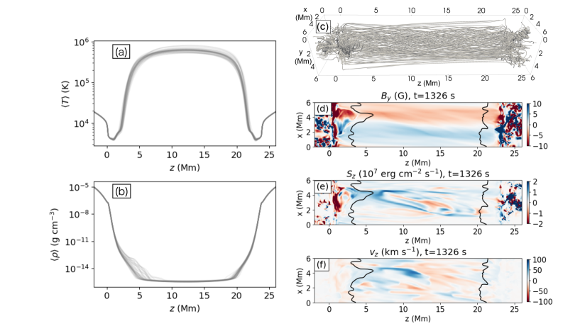
Figure 1: Panel (a) and (b): the probability distributions of the $xy$-averaged temperature $\langle T\rangle$ and mass density $\langle\rho\rangle$ for $t$ and $z$. Panel (c)–(f): snapshots ($t=1,326\ \mathrm{s}$) of magnetic field lines, $B_{y}$, $S_{z}$, and $v_{z}$ on the $xz$-plane at $y=1\ \mathrm{Mm}$ in the presence of the magnetic tornado. The black contours in panel (d)–(f) indicate the transition region height where $T=80,000\ \mathrm{K}$.

2.2 Synthetic Emission

Chromospheric swirls have frequently been observed in Ca II IR and H$\alpha$ by ground-based telescopes such as SST/CRISP (e.g., Shetye et al., 2019; Dakanalis et al., 2022). Additionally, an observation through the Interface Region Imaging Spectrograph (IRIS, De Pontieu et al., 2014) has detected swirls in Mg II line (Park et al., 2016). In this paper, we synthesize Ca II 8542 Å, Ca II K, and Mg II k spectral lines, utilizing the publicly available RH1.5D code (Uitenbroek, 2001; Pereira & Uitenbroek, 2015). This code can treat optically thick line formation under non-LTE condition and partial frequency redistribution, which is critical to modelling the chromospheric spectral lines in detail. The 1.5D (column-by-column) treatment of radiation transport is generally valid except at the cores of strong chromospheric lines such as Ca II K and Mg II k where the effects of lateral radiation (3D) transport become important (Sukhorukov & Leenaarts, 2017; Bjørgen et al., 2018). However, since the aim of this paper is not a direct comparison of the synthesized observables with actual observations and owing to the substantially high time complexity of 3D non-LTE radiative transfer, the benefits of the 1.5D approach far outweigh its limitations (Pereira & Uitenbroek, 2015). Moreover, as shown in Sec.3, the 1.5D approach distinctly reproduces the signature of the swirls in the chromosphere.

For the coronal response, we synthesize the EUV emission as observed in the AIA 171 Å channel. Furthermore, the 174 Å channel of the Extreme Ultraviolet Imager (EUI; Rochus et al., 2020) on board Solar Orbiter (SolO; Müller et al., 2020) is also calculated. The coronal emission is calculated assuming the optically thin approximation under ionization equilibrium, following a methodology similar to that of Chen et al. (2021). The emission $I_{\mathrm{corona}}$ is given as:

$$I_{\mathrm{corona}}=\int n_{{\color[rgb]{0,0,0}\mathrm{e}}}n_{{\color[rgb]{0,0,0}\mathrm{H}}}K(T)ds,$$ (5)

where $s$ is the line of sight direction, $n_{e}$ is electron number density, $n_{H}$ is hydrogen number density, and $K(T)$ is the contribution function corresponding to the AIA 171 Å and EUI 174 Å channels computed using the FoMo code (Van Doorsselaere et al., 2016). For a direct comparison between the synthesized emission and observations, we consider the pixel sizes of the instruments. The AIA instrument has a spatial resolution of $\approx$ $1.2{\color[rgb]{0,0,0}"}$, while the EUI instrument has $\approx$ $0.4{\color[rgb]{0,0,0}"}$. Following the procedure outlined by Breu et al. (2022), we resample the synthesized emissions by summing up neighboring pixel patches from the numerical model to match the instrumental spatial scale. For simplicity, we did not convolve with the point spread function.

3 Results

3.1 Simulation Overview

Figure 1a and b depict the probability distribution of horizontally averaged temperature $T$ and mass density $\rho$, denoted as $\langle T\rangle$ and $\langle\rho\rangle$, respectively. It is worth noting that we define the angle brackets $\langle\rangle$ as representing the $xy$-averaging. $\langle T\rangle$ ranges from $0.5\ \mathrm{MK}$ to $0.8\ \mathrm{MK}$, while locally, it exceeds $1\ \mathrm{MK}$. Furthermore, $\langle\rho\rangle$ reveals that chromospheric plasma on the left-hand side extends to higher altitudes ($z=3$–$6\ \mathrm{Mm}$) compared to the right-hand side. This result arises from a chromospheric jet initiated, which is revisited later.

During the analyzed period, a magnetic tornado is generated by photospheric vortex flows, which is the same triggering mechanism as presented in many previous simulations (Kuniyoshi et al., 2023; Silva et al., 2024). Figure 1c displays a snapshot of magnetic field lines when the magnetic tornado is produced. It exhibits a coherently twisted feature extending from the left-hand side of the surface ($z=0\ \mathrm{Mm}$) to the entire coronal volume. Figure 2d–f illustrates snapshots of the $y$-component of the magnetic field $B_{y}$, vertical Poynting flux $S_{z}$ (where $S_{z}=(B_{x}^{2}+B_{y}^{2})v_{z}/4\pi-(v_{x}B_{x}+v_{y}B_{y})B_{z}/4\pi$), and vertical velocity $v_{z}$ on the $xz$-plane at $y=1\ \mathrm{Mm}$, with the transition region height where $T={\color[rgb]{0,0,0}80,000}\ \mathrm{K}$. These quantities clearly depict typical features of magnetic tornadoes. In the region $1\ \mathrm{Mm}<z<3\ \mathrm{Mm}$, highly twisted $B_{y}$ with an absolute value reaching over $10\ \mathrm{G}$ is observed, extending to the coronal height. Through this region, an amplified vertical Poynting flux $S_{z}$ exceeding $1\times 10^{7}\ \mathrm{erg\ cm^{-2}\ s^{-1}}$ is channeled into the corona. Additionally, the transition region height increases just above this region to $6\ \mathrm{Mm}$, from which enhanced vertical velocity $v_{z}$ surpassing $50\ \mathrm{km\ s^{-1}}$ extends into the corona. They are the features of the chromospheric jet driven by the Lorentz force accompanying the magnetic tornado, which is consistent with the previous simulation (Iijima & Yokoyama, 2017; Dey et al., 2024).

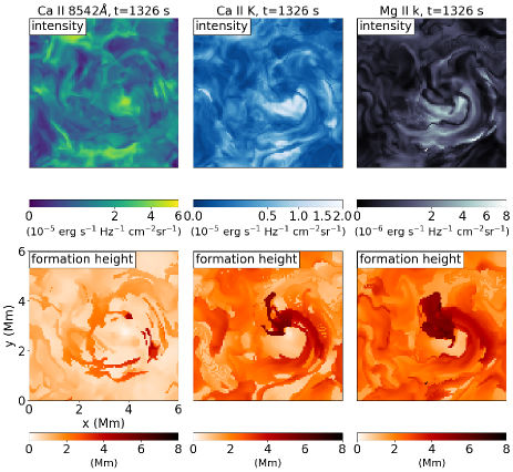
Figure 2: Top row: Snapshots ($t=1,326\ \mathrm{s}$) of chromospheric emissions in Ca II 8542 Å, Ca II K, and Mg II k as observed from the coronal apex ($z=12\ \mathrm{Mm}$). Bottom row: The formation heights of the emissions. The associated animation shows the temporal evolution over a period from $t=1,254\ \mathrm{s}$ to $t=1,350\ \mathrm{s}$.

3.2 Magnetic Tornado Synthesis

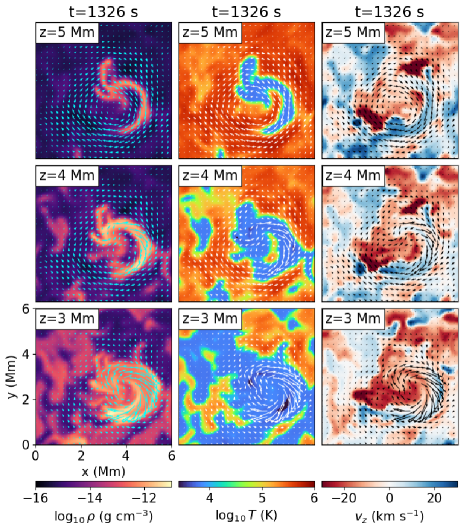
Figure 3: Horizontal slices of $\rho$, $T$, and $v_{z}$ at $z=5\ \mathrm{Mm}$ (top row), $z=4\ \mathrm{Mm}$ (middle row), and $z=3\ \mathrm{Mm}$ (bottom row) at $t=1,326\ \mathrm{s}$. The associated animation shows the temporal evolution over a period from $t=1,254\ \mathrm{s}$ to $t=1,350\ \mathrm{s}$.

In this section, we synthesize the chromospheric and coronal emissions corresponding to the magnetic tornado. The first row of Figure 2 displays the chromospheric synthesis of Ca II 8542 Å, Ca II K, and Mg II k line cores as observed from the negative $z$-direction at $z=12\ \mathrm{Mm}$. These panels and associated animation illustrate that the magnetic tornado can be observed as a rotating swirl-like feature with arc structures, with a diameter of about $3\ \mathrm{Mm}$. The second row shows the $\tau=1$ formation height corresponding to the wavelength of the images shown in the top row. They reveal that the synthesized swirl originating from the magnetic tornado are formed between $z=3$–$5\ \mathrm{Mm}$. In Figure 3, horizontal slices of $\rho$, $T$, and $v_{z}$ at corresponding heights $z=3$–${\color[rgb]{0,0,0}5}\ \mathrm{Mm}$ are displayed, with horizontal magnetic field ($B_{x},B_{y}$) in arrows. These quantities have displayed that the synthesized swirl is characterized by the chromospheric jet with denser and cooler structures than surrounding plasma, upflowing through the twisted magnetic field (see also the corresponding animation).

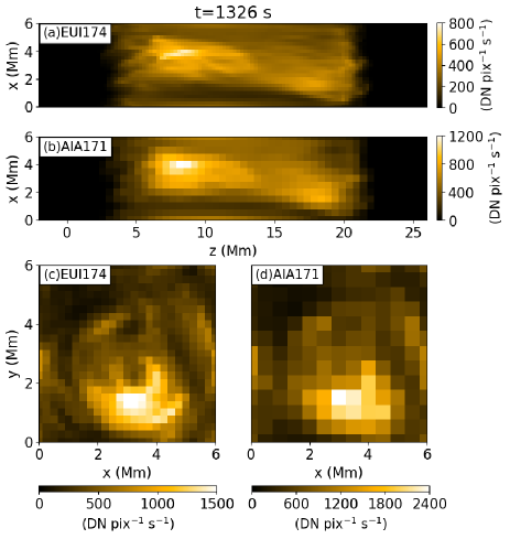
Figure 4: Snapshots ($t=1,326\ \mathrm{s}$) of synthesized emissions in the SolO/EUI $174$ Å and SDO/AIA $171$ Å channel as seen from the negative $y$-direction (panel (a)–(b)) and from the negative $z$-direction at $z=12\ \mathrm{Mm}$. The corresponding animation shows the temporal evolution over a period from $t=1,254\ \mathrm{s}$ to $t=1,350\ \mathrm{s}$.

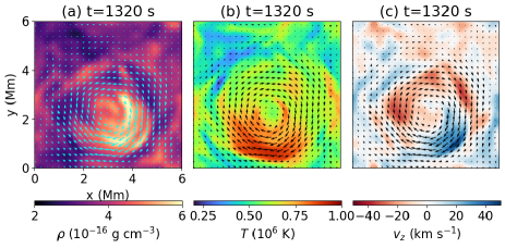
Figure 5: Horizontal maps of (a) mass density $\rho$, (b) temperature $T$, and (c) vertical velocity $v_{z}$ are displayed in color, with the horizontal magnetic field $(B_{x},B_{y})$ represented by arrows. These maps are averaged over the coronal height range $7\ \mathrm{Mm}<z<12\ \mathrm{Mm}$ at $t=1,326\ \mathrm{s}$. The associated animation shows the temporal evolution over a period from $t=1,254\ \mathrm{s}$ to $t=1,350\ \mathrm{s}$.

Figure 4a–b present the synthesized lower coronal emission as observed by the SolO/EUI 174 Å and SDO/AIA 171 Å channels from the negative $y$-direction at the same time as the chromospheric lines. These panels and associated animations reveal that the EUV brightening occurs within the range of $6\ \mathrm{Mm}\leq z\leq 9\ \mathrm{Mm}$. Although this simulation disregards the curvature of the coronal loop, assuming the coronal loop as semicircular, the corresponding formation altitude from the surface ranges from $5\ \mathrm{Mm}$ to $8\ \mathrm{Mm}$. Figure 4c–d present snapshots of the same coronal emissions at the same time, observed from different viewing angle (the negative $z$-direction from $z=12\ \mathrm{Mm}$). Both emissions exhibit coronal brightening with a width of approximately $\sim 2\ \mathrm{Mm}$, centered at $(x,y)=(3\ \mathrm{Mm},1\ \mathrm{Mm})$. It is important to note that we do not account for EUV absorption by chromospheric materials (such as H I, He I, and He II), as there are no chromospheric jets or prominences generated in front of the coronal brightening along the line of sight of the synthesized emissions.

To analyze the thermal properties of this brightening, Figure 5a–c present the horizontal slices of $T$, $\rho$ and $v_{z}$ with $(B_{x},B_{y})$ in arrows, averaged over the coronal height $7\ \mathrm{Mm}\leq z\leq 12\ \mathrm{Mm}$. These maps and corresponding animation suggest that the brightening occurs within the twisted magnetic field generated by the magnetic tornado, resulting from the local enhancement of mass density and temperature in the region where $2\ \mathrm{Mm}<x<5\ \mathrm{Mm}$ and $1\ \mathrm{Mm}<y<3\ \mathrm{Mm}$. The positional correspondence between the local enhancement of $\rho$ and $v_{z}$ indicates that the coronal mass is being supplied by the chromospheric jet triggered by the magnetic tornado (see also Figure 1f). The temperature increase is possibly caused by component magnetic reconnection between internally adjacent field lines within the twisted magnetic field, a phenomenon that will be investigated in our future work. From these results, we can infer that the coronal response to magnetic tornadoes can be observed as local brightenings just above chromospheric swirls.

4 Discussion

In accordance with previous studies (Wedemeyer-Böhm et al., 2012; Tziotziou et al., 2018), our synthesis has illustrated that a magnetic tornado can be observed as a swirl in chromospheric lines. The synthesized swirl in Ca II lines corresponds to previous observations by SST/CRISP, exhibiting a similar diameter of $\sim 2\ \mathrm{Mm}$ (e.g., Shetye et al., 2019). Our study suggests that chromospheric swirls can also be observed in Mg II k line. This result aligns with previous IRIS observations by Park et al. (2016), which revealed the signature of the chromospheric swirl obtained in a sit-and-stare mode of the Mg II k 2796 Å line. Considering that the diameter of our swirl is sufficiently larger than the spatial resolution of IRIS ($0.4{\color[rgb]{0,0,0}"}$ De Pontieu et al., 2014), our synthesis indicates that swirls can be observed in the slit-jaw images (SJIs) in the Mg II k filter.

We have also analyzed the coronal response to the magnetic tornado, as observed in the SolO/EUI 174 Å and SDO/AIA 171 Å channels. From our synthesis, a brightening in both channels is observed above the chromospheric swirl. This result well corresponds to the previous observation by Wedemeyer-Böhm et al. (2012), conducting the coordinated observation by SST/CRISP Ca II 8542 Å line and SDO/AIA 171 Å channel. On the other hand, our result contradicts the observations by Tziotziou et al. (2018), which shows a darkening in AIA 171 Å channel above a chromospheric swirl observed in SST/CRISP Ca II 8542 Å and H$\alpha$ lines. This discrepancy may arise because chromospheric materials such as coronal rains or fibrils positioned over the magnetic tornado, obscure its coronal brightening.

The altitude of the synthesized coronal brightening from the surface ranges from $5\ \mathrm{Mm}$ to $8\ \mathrm{Mm}$ when we assume our coronal loop to be semi-circular. Interestingly, the lower limit is consistent with the reported formation height of the campfires, at least a portion of which is caused by the coronal EUV brighteings observed by SolO/EUI 174 Å channel (Berghmans et al., 2021). The promising mechanisms for the campfires is the reconnection of low-lying or emerging loops, facilitated by their height correspondence (Hansteen et al., 2014; Chen et al., 2021; Panesar et al., 2021). However, our results propose that magnetic tornadoes are likely to be alternative mechanisms to produce the campfires because there are no low-lying or emerging loops at coronal heights in our simulation (see Figure 1c). This supports the recent observation proposing that the physics behind all the campfires are likely not the same because some have an IRIS counterpart while others do not (Nelson et al., 2023). Therefore, to elucidate the origin of campfires, coordinated observations by ground-based telescopes such as the SST/CRISP or Goode Solar Telescope (GST; Cao et al., 2010)/Fast Imaging Solar Spectrograph (FISS Chae et al., 2013) for the chromosphere and the SolO/EUI for the corona are crucial. If magnetic tornadoes indeed trigger campfires, chromospheric swirls should be observable just below the EUV brightenings.

It is worth noting that spectropolarimetric synthesis of magnetic tornadoes is also performed using the dataset computed by the RAMENS code (Matsumoto et al., 2023). These studies have predicted arc-like linear polarisation signals originating from the highly twisted magnetic field lines, which can be observed by the upcoming polarimetric observations such as SUNRISE III/Sunrise Chromospheric Infrared spectro-Polarimeter (SCIP; Katsukawa et al., 2020), Daniel K. Inouye Solar Telescope (DKIST; Rimmele et al., 2020) and European Solar Telescope (EST; Quintero Noda et al., 2022).

Numerical computations were carried out on the Cray XC50 at the Center for Computational Astrophysics (CfCA), National Astronomical Observatory of Japan. S.B. is supported by NASA contract NNG09FA40C (IRIS).The simulations were performed on resources provided by Sigma2 – the National Infrastructure for High Performance Computing and Data Storage in Norway. T.Y. is supported by the JSPS KAKENHI Grant Number JP21H01124, JP20KK0072, and JP21H04492. This work was supported by NAOJ Research Coordination Committee, NINS, Grant Number NAOJ-RCC-2301-0301.

References

- Battaglia et al. (2021) Battaglia, A. F., Canivete Cuissa, J. R., Calvo, F., Bossart, A. A., & Steiner, O. 2021, A&A, 649, A121, doi: 10.1051/0004-6361/202040110
- Berger et al. (1995) Berger, T. E., Schrijver, C. J., Shine, R. A., et al. 1995, ApJ, 454, 531, doi: 10.1086/176504
- Berghmans et al. (2021) Berghmans, D., Auchère, F., Long, D. M., et al. 2021, A&A, 656, L4, doi: 10.1051/0004-6361/202140380
- Bjørgen et al. (2018) Bjørgen, J. P., Sukhorukov, A. V., Leenaarts, J., et al. 2018, A&A, 611, A62, doi: 10.1051/0004-6361/201731926
- Breu et al. (2022) Breu, C., Peter, H., Cameron, R., et al. 2022, A&A, 658, A45, doi: 10.1051/0004-6361/20214145110.48550/arXiv.2112.11549
- Cao et al. (2010) Cao, W., Gorceix, N., Coulter, R., et al. 2010, Astronomische Nachrichten, 331, 636, doi: 10.1002/asna.201011390
- Chae et al. (2013) Chae, J., Park, H.-M., Ahn, K., et al. 2013, Sol. Phys., 288, 1, doi: 10.1007/s11207-012-0147-x
- Chen et al. (2021) Chen, Y., Przybylski, D., Peter, H., et al. 2021, A&A, 656, L7, doi: 10.1051/0004-6361/202140638
- Dakanalis et al. (2022) Dakanalis, I., Tsiropoula, G., Tziotziou, K., & Kontogiannis, I. 2022, A&A, 663, A94, doi: 10.1051/0004-6361/202243236
- De Pontieu et al. (2014) De Pontieu, B., Title, A. M., Lemen, J. R., et al. 2014, Sol. Phys., 289, 2733, doi: 10.1007/s11207-014-0485-y
- Dey et al. (2024) Dey, S., Chatterjee, P., & Erdelyi, R. 2024, arXiv e-prints, arXiv:2404.16096, doi: 10.48550/arXiv.2404.16096
- Díaz Baso et al. (2021) Díaz Baso, C. J., de la Cruz Rodríguez, J., & Leenaarts, J. 2021, A&A, 647, A188, doi: 10.1051/0004-6361/202040111
- Edlén (1943) Edlén, B. 1943, ZAp, 22, 30
- Hansteen et al. (2015) Hansteen, V., Guerreiro, N., De Pontieu, B., & Carlsson, M. 2015, ApJ, 811, 106, doi: 10.1088/0004-637X/811/2/106
- Hansteen et al. (2014) Hansteen, V., De Pontieu, B., Carlsson, M., et al. 2014, Science, 346, 1255757, doi: 10.1126/science.1255757
- Iijima (2016) Iijima, H. 2016, PhD thesis, Department of Earth and Planetary Environmental Science, The Univ. of Tokyo
- Iijima & Yokoyama (2017) Iijima, H., & Yokoyama, T. 2017, ApJ, 848, 38, doi: 10.3847/1538-4357/aa8ad1
- Katsukawa et al. (2020) Katsukawa, Y., del Toro Iniesta, J. C., Solanki, S. K., et al. 2020, in Society of Photo-Optical Instrumentation Engineers (SPIE) Conference Series, Vol. 11447, Ground-based and Airborne Instrumentation for Astronomy VIII, ed. C. J. Evans, J. J. Bryant, & K. Motohara, 114470Y, doi: 10.1117/12.2561223
- Klimchuk (2006) Klimchuk, J. A. 2006, Sol. Phys., 234, 41, doi: 10.1007/s11207-006-0055-z
- Kuniyoshi et al. (2023) Kuniyoshi, H., Shoda, M., Iijima, H., & Yokoyama, T. 2023, ApJ, 949, 8, doi: 10.3847/1538-4357/accbb8
- Kuniyoshi et al. (2024) Kuniyoshi, H., Shoda, M., Morton, R. J., & Yokoyama, T. 2024, ApJ, 960, 118, doi: 10.3847/1538-4357/ad1038
- Leenaarts (2020) Leenaarts, J. 2020, Living Reviews in Solar Physics, 17, 3, doi: 10.1007/s41116-020-0024-x
- Lemen et al. (2012) Lemen, J. R., Title, A. M., Akin, D. J., et al. 2012, Sol. Phys., 275, 17, doi: 10.1007/s11207-011-9776-8
- Matsumoto et al. (2023) Matsumoto, T., Kawabata, Y., Katsukawa, Y., Iijima, H., & Quintero Noda, C. 2023, MNRAS, 523, 974, doi: 10.1093/mnras/stad1509
- Müller et al. (2020) Müller, D., St. Cyr, O. C., Zouganelis, I., et al. 2020, A&A, 642, A1, doi: 10.1051/0004-6361/202038467
- Nelson et al. (2023) Nelson, C. J., Auchère, F., Aznar Cuadrado, R., et al. 2023, A&A, 676, A64, doi: 10.1051/0004-6361/202346144
- Panesar et al. (2021) Panesar, N. K., Tiwari, S. K., Berghmans, D., et al. 2021, ApJ, 921, L20, doi: 10.3847/2041-8213/ac3007
- Park et al. (2016) Park, S. H., Tsiropoula, G., Kontogiannis, I., et al. 2016, A&A, 586, A25, doi: 10.1051/0004-6361/201527440
- Parker (1983) Parker, E. N. 1983, ApJ, 264, 642, doi: 10.1086/160637
- Pereira & Uitenbroek (2015) Pereira, T. M. D., & Uitenbroek, H. 2015, A&A, 574, A3, doi: 10.1051/0004-6361/201424785
- Pesnell et al. (2012) Pesnell, W. D., Thompson, B. J., & Chamberlin, P. C. 2012, Sol. Phys., 275, 3, doi: 10.1007/s11207-011-9841-3
- Pevtsov et al. (2003) Pevtsov, A. A., Fisher, G. H., Acton, L. W., et al. 2003, ApJ, 598, 1387, doi: 10.1086/378944
- Quintero Noda et al. (2022) Quintero Noda, C., Schlichenmaier, R., Bellot Rubio, L. R., et al. 2022, A&A, 666, A21, doi: 10.1051/0004-6361/202243867
- Rempel (2017) Rempel, M. 2017, ApJ, 834, 10, doi: 10.3847/1538-4357/834/1/10
- Rimmele et al. (2020) Rimmele, T. R., Warner, M., Keil, S. L., et al. 2020, Sol. Phys., 295, 172, doi: 10.1007/s11207-020-01736-7
- Rochus et al. (2020) Rochus, P., Auchère, F., Berghmans, D., et al. 2020, A&A, 642, A8, doi: 10.1051/0004-6361/201936663
- Scharmer et al. (2003) Scharmer, G. B., Bjelksjo, K., Korhonen, T. K., Lindberg, B., & Petterson, B. 2003, in Society of Photo-Optical Instrumentation Engineers (SPIE) Conference Series, Vol. 4853, Innovative Telescopes and Instrumentation for Solar Astrophysics, ed. S. L. Keil & S. V. Avakyan, 341–350, doi: 10.1117/12.460377
- Scharmer et al. (2008) Scharmer, G. B., Narayan, G., Hillberg, T., et al. 2008, ApJ, 689, L69, doi: 10.1086/595744
- Schrijver et al. (1997) Schrijver, C. J., Hagenaar, H. J., & Title, A. M. 1997, ApJ, 475, 328, doi: 10.1086/303528
- Shetye et al. (2019) Shetye, J., Verwichte, E., Stangalini, M., et al. 2019, ApJ, 881, 83, doi: 10.3847/1538-4357/ab2bf9
- Silva et al. (2024) Silva, S. S. A., Verth, G., Rempel, E. L., et al. 2024, ApJ, 963, 10, doi: 10.3847/1538-4357/ad1403
- Sukhorukov & Leenaarts (2017) Sukhorukov, A. V., & Leenaarts, J. 2017, A&A, 597, A46, doi: 10.1051/0004-6361/201629086
- Tziotziou et al. (2018) Tziotziou, K., Tsiropoula, G., Kontogiannis, I., Scullion, E., & Doyle, J. G. 2018, A&A, 618, A51, doi: 10.1051/0004-6361/201833101
- Tziotziou et al. (2023) Tziotziou, K., Scullion, E., Shelyag, S., et al. 2023, Space Sci. Rev., 219, 1, doi: 10.1007/s11214-022-00946-8
- Uitenbroek (2001) Uitenbroek, H. 2001, ApJ, 557, 389, doi: 10.1086/321659
- Van Doorsselaere et al. (2016) Van Doorsselaere, T., Antolin, P., Yuan, D., Reznikova, V., & Magyar, N. 2016, Frontiers in Astronomy and Space Sciences, 3, 4, doi: 10.3389/fspas.2016.00004
- Van Doorsselaere et al. (2020) Van Doorsselaere, T., Srivastava, A. K., Antolin, P., et al. 2020, Space Sci. Rev., 216, 140, doi: 10.1007/s11214-020-00770-y
- Wedemeyer-Böhm et al. (2012) Wedemeyer-Böhm, S., Scullion, E., Steiner, O., et al. 2012, Nature, 486, 505, doi: 10.1038/nature11202
- Withbroe & Noyes (1977) Withbroe, G. L., & Noyes, R. W. 1977, ARA&A, 15, 363, doi: 10.1146/annurev.aa.15.090177.002051