Deep generative modelling of canonical ensemble with differentiable thermal properties

Abstract

We propose a variational modelling method with differentiable temperature for canonical ensembles. Using a deep generative model, the free energy is estimated and minimized simultaneously in a continuous temperature range. At optimal, this generative model is a Boltzmann distribution with temperature dependence. The training process requires no dataset, and works with arbitrary explicit density generative models. We applied our method to study the phase transitions (PT) in the Ising and XY models, and showed that the direct-sampling simulation of our model is as accurate as the Markov Chain Monte Carlo (MCMC) simulation, but more efficient. Moreover, our method can give thermodynamic quantities as differentiable functions of temperature akin to an analytical solution. The free energy aligns closely with the exact one to the second-order derivative, so this inclusion of temperature dependence enables the otherwise biased variational model to capture the subtle thermal effects at the PTs. These findings shed light on the direct simulation of physical systems using deep generative models.

The canonical ensemble is for a system in thermal equilibrium with a heat bath, where the temperature, as a principal thermodynamic variable, determines the probability distribution of states. The key to calculating macroscopic thermal properties is the partition function:

$$\mathcal{Z}=\int\exp(-\beta E(\mathbf{x}))d\mathbf{x},~{}F=-T\log\mathcal{Z},$$ (1)

where $E$ is the energy function, $\beta$ is the inverse of the temperature $T$, $F$ is the Helmholtz free energy. For example, after obtaining the partition function $\mathcal{Z}$, the mean energy and the heat capacity can be readily calculated as

$$\langle E\rangle=-\frac{\partial\log\mathcal{Z}}{\partial\beta},~{}C_{v}=\beta^{2}\frac{\partial^{2}\log\mathcal{Z}}{\partial\beta^{2}}.$$ (2)

For most physical systems, it is impossible to analytically solve $\mathcal{Z}$: an exact enumeration belongs to the class of #P-hard [1]. In practical calculations, it is common to approximate $\mathcal{Z}$ numerically[2, 3]. However, even numerical approximation remains highly challenging, especially for systems undergoing phase transitions (PTs), where the partition function must account for a large number of metastable states.

Due to the complexity of $\mathcal{Z}$, sample-based methods are widely used in numerical calculations, among which the Markov Chain Monte Carlo (MCMC) method holds prominence. The MCMC method is an importance sampling technique giving the Boltzmann distribution in the canonical ensemble:

$$p(\mathbf{x})=\frac{\exp(-\beta E(\mathbf{x}))}{\mathcal{Z}}.$$ (3)

It can provide the prevailing sample configurations at a microscopic level, which are often absent in partition function approaches. This microscopic information is very valuable, e.g., in the identification of intermediate states in chemical reactions. Macroscopic properties can also be estimated by averaging the samples [4], namely, statistical averaging. An inherent limitation of MCMC is its efficiency. Due to the Markov chain structure of the rejection sampling, it takes multiple timesteps to produce an independent and identically distributed (i.i.d.) sample, which prohibits the MCMC from performing direct sampling. [5]. This autocorrelation problem becomes even worse near PTs [5, 6]. Additionally, unlike the explicit temperature dependence in the partition function, the MCMC method typically requires more computational effort for results on multiple temperature points, further diminishing its overall efficiency.

Recently, the explicit density generative model, a deep learning method, was introduced to overcome the efficiency limitation of MCMC [7, 8, 9]. It can direct give i.i.d. samples from parameterized distributions to compute statistical averages [7]. Some of the models can also provide the free energy estimation [8, 10], which is deemed challenging for MCMC. However, the limitation of temperature dependence persists, as one still has to train separate models for each temperature point, similar to MCMC. What makes it worse than MCMC is that, during this discrete-temperature training, the functional dependence of free energy and other thermodynamic quantities on temperature is broken, a major trade-off due to the absence of a differentiable $\mathcal{Z}$. In the case of MCMC, despite its inefficiency due to discrete temperature, one can still rely on its unbiased estimation to get accurate results. However, deep learning models, being variational models, may exhibit biases and lack physical fidelity. Consequently, the accuracy of deep generative models is often inadequate for directly representing the ensemble, particularly during phase transitions. When applying these variational models, one usually has to compensate with the aid of the MCMC rejection [8] or multiple-temperature training like annealing [10].

Variational temperature-differentiable optimization.

In this Letter, we propose a general framework of directly modelling the canonical ensemble in a continuous temperature range. The resulting deep generative model is a direct-sampling model of the target Boltzmann distribution with temperature dependence. As the model is differentiable with temperature, the estimates, including the free energy and the partition function, can be differentiated in a similar way to an analytical solution.

First, considering a single temperature, one can minimize the reverse Kullback-Leibler divergence (KLD) [11] to optimize an explicit density generative model, i.e.,

$$\begin{aligned} D_{KL}(q_{\theta}||p)&=\mathop{\mathbb{E}}_{\mathbf{x}\sim q_{\theta}}\log\frac{q_{\theta}(\mathbf{x})}{p(\mathbf{x})}\\ &=\log\mathcal{Z}+\mathop{\mathbb{E}}_{\mathbf{x}\sim q_{\theta}}\left[\log q_{\theta}(\mathbf{x})+\beta E(\mathbf{x})\right],\end{aligned}$$ (4)

where $q_{\theta}$ is the model distribution, and $p$ is the Boltzmann distribution (Eq. (3)) at this temperature. After optimization, the model $q_{\theta}$ is an approximation of $p$. Additional, because the $D_{KL}\geq 0$, the statistical average, $\mathbb{E}_{\mathbf{x}\sim q_{\theta}}[\log q_{\theta}(\mathbf{x})+\beta E(\mathbf{x})]$, has a variational lower bound at $-\log\mathcal{Z}$, it can be used as an estimate of the partition function in Eq. (1) [8, 10]. This has been successfully demonstrated on various applications [12, 13, 14, 15, 16]. However, as the true Boltzmann distribution is a function of temperature, training schemes optimizing on a single temperature may be biased and unphysical. This is usually demonstrated as the hardness of optimizing Eq. (4).

Here, we propose that approximating the temperature-dependent Boltzmann distribution by training in a differentiable temperature range. Conventionally, finding the temperature-dependent Boltzmann distribution involves the following free energy minimization problem.

$$\begin{split}\min_{q_{\theta}}\sum_{\{\mathbf{x}\}}\left[1/\beta\cdot q_{\theta}(\mathbf{x},\beta)\log q_{\theta}(\mathbf{x},\beta)+q_{\theta}(\mathbf{x},\beta)E(\mathbf{x})\right],\\ \text{s.t.}~{}\sum_{\{\mathbf{x}\}}q_{\theta}(\mathbf{x},\beta)=1,~{}\forall\beta,\end{split}$$ (5)

One can see that the Boltzmann distribution in Eq. (3) is the solution [17].

Next, we use an explicit density model as the variational $q_{\theta}$, and convert Eq. (5) into a similar form as Eq. (4), so that we can perform deep-learning training. As explicit density models are normalized distributions, the normalization is naturally met. The summation over $\{\bm{x}\}$ becomes an estimation over $q_{\theta}$. And this minimum is also the minimum of an integration of the free energy. We further turn this integration into an estimation over an equal-probability distribution of $\beta$. Thus, the following loss function is equivalent to the free energy minimization in Eq. (5):

$$\mathcal{L}=\mathop{\mathbb{E}}_{\begin{subarray}{c}\beta\sim\text{U}\\ \mathbf{x}\sim q_{\theta}(\cdot,\beta)\end{subarray}}\left[\log q_{\theta}(\mathbf{x},\beta)+\beta E(\mathbf{x})\right]=\mathop{\mathbb{E}}_{\beta\sim\text{U}}\left[-\log\bar{\mathcal{Z}}(\beta)\right].$$ (6)

One can perform the stochastic gradient descent (SGD) [18, 19] to optimize it. Gradients can be obtained from the computational graph and automatic differentiation, which are widely used in deep learning [20]. After training, we obtain $q_{\theta}$ as a variational approximation of the Boltzmann distribution with differentiable temperature dependence.

Compared to Eq. (4), this variational temperature-differentiable (VaTD) loss function is an integration of the reverse KLD over a continuous temperature range. Using the reverse KLD as loss, this training doesn’t require any dataset, because the sample $\mathbf{x}$ is drawn from a direct-sample generative model $q_{\theta}$. Another benefit is that one gets a temperature-differentiable estimate of the free energy: $\log\bar{\mathcal{Z}}(\beta)$, so its derivatives with respect to temperature, e.g., the mean energy in Eq. (2) and heat capacity in Eq. (2), can be readily calculated using automatic differentiation. Other thermodynamic quantities, e.g., the magnetization, can be also estimated by computing the statistical averages of directly sampled batches, and they are also functions of differentiable temperature.

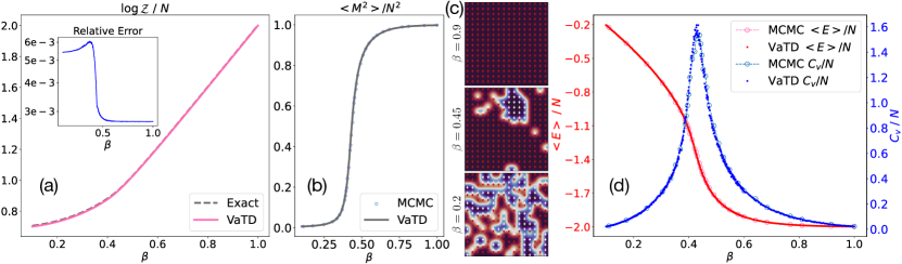
Figure 1: (a) The exact and estimated free energy of the 2D Ising model on a $16\times 16$ PBC square lattice, and the relative error between the two (inset). The temperature factor (-$T$) is removed for better comparison. (b) The estimated square magnetization of the Ising model. (c) Configurations directly sampled from the learned model at three temperatures, with background color as a continuous interpolation of the discrete site for better visualization. (d) The mean energy and heat capacity of the Ising model, estimated using the differentiation of the free energy, compared with the results obtained from the MCMC simulation.

One concern is that $q_{\theta}$ may not be flexible enough to cover the whole space of probability distribution, which may result in sub-optimal solutions for Eq. (5) and miss the Boltzmann distribution. However, this problem can be overcome by employing sufficiently large neural network models to representing $q_{\theta}$, as guaranteed by the universal approximation theorem [21]. Additionally, compared with directly constructing a specific model always following the Boltzmann distribution [22], our method comes with nearly no restriction on the model, and thus has maximum fitting ability. In the VaTD training, the model initially starts as a random non-Boltzmann distribution, and is optimized to be a Boltzmann distribution, which extends the generality of the proposed framework. One can choose specially tailored models for different applications.

In performing SGD, one should notice that the gradients of Eq. (6) is not trivial. As the model parameters $\theta$ are used in the expectation operator, the nice form of statistical averaging will be lost in the gradients. To overcome this, two numerical methods, namely reparameterization and reinforce estimation, have been proposed [23]. They enable the swapping of the derivative operation with the expectation operation, thereby converting the derivative calculations of statistical averages into the statistical averaging of derivatives. The same problem reoccurs when calculating the derivative of estimated thermal differentiable function with respect to $\beta$. This can be solved again by using these two methods. Typically only the first-order forms of these two methods are presented for purpose of training. We extend them to the second order in appendix [17]. It is worth noting that higher-order generalizations are feasible as long as the neural network remains continuous.

Numerical experiments.

In the numerical experiments, we demonstrate our method using two famous statistical models: two-dimensional Ising and XY models. The former one uses a discrete-variable model, PixelCNN [24], while the latter one uses a continuous-variable model, the normalizing flow (NF).

Our 2D Ising model is on a $16\times 16$ square lattice with periodic boundary conditions (PBC). The energy function is given by $E(\mathbf{x})=-\sum_{<i,j>}x_{i}x_{j}$, where $<i,j>$ means the two spins are nearest neighbors on the lattice. Variables of Ising are discrete, i.e., $x_{i}\in\{-1,1\}$ where $1$ and $-1$ stand for spin-up and -down, respectively.

For Ising, we chose the PixelCNN model [24], which is an explicit density generative model for discrete-variable distributions. Its probability distribution is decomposed into the product of a series of conditional probability distributions, i.e., $q_{\theta}(\mathbf{x},\beta)=\prod_{i}q_{\theta}(x_{i}|x_{0},\cdots,x_{i-1};\beta)$. The conditional distribution we chose is the Bernoulli distribution, $x_{i}\sim B(1,p)$, where $p$ is the probability of a spin-up state, obtained from a ResNet [25] given the preceding variables $\{x_{0},\cdots,x_{i-1}\}$ and $\beta$. To have a unified input form, we repeated $\beta$ to match the size of $\{x_{0},\cdots,x_{i-1}\}$, and then concatenated them along the channel dimension. The PixelCNN model generates variables sequentially, one at a time. During each step, a variable is stochastically sampled from the Bernoulli distribution. The conditional causality is established through the dependence of the Bernoulli parameter $p$ on the preceding variables. The model was trained in a temperature range of $\beta\in[0.05,1.2]$. To eliminate the $\mathbb{Z}_{2}$ symmetry, we fixed the first spin to be spin-up.

After training, the PixelCNN model can perform direct sampling, and the sampled batches were used for statistical averaging. In Fig. 1(a), we estimated the free energy as a continuous function of temperature using Eq. (6). As the 2D Ising can be analytically solved [26], we compared our numerical results with the exact free energy at each temperature point in Fig. 1(a), and found that the relative errors are small, with the maximum happening near the PT region where the system exhibits long-range correlations and multiple meta-stable states. Similarly, we also calculated the square magnetization, which is in excellent agreement with the result obtained by the MCMC simulation, as shown in Fig. 1(b). This indicates our method has comparable accuracy with MCMC, but is more efficient. The sampled configurations also provide valuable insights into the microscopic behaviors of the system, and demonstrates that the underlying physical transition is successfully captured. In Fig. 1(c), we observe that the trained model effectively captures the microscopic changes at lower $\beta$, where the uniform spin direction gradually collapses. Hence, our method trained a neural network model that undergoes the same microscopic thermal transition as the target Ising model.

To further prove that our model successfully captures the subtle thermal transitions near the PTs, we computed mean energy and heat capacity, which are the derivatives of the free energy, as shown in Eq. (2), and compared with the unbiased MCMC results in Fig. 1(d). Overall, our results agree very well with those from the MCMC simulation, with only slight deviations observed near the PT region. This implies that the estimated free energy aligns closely with the exact one to the second-order derivative. Moverover, comparing with statistical averaging using direct sampling, these derivatives have advantage in efficiency and accuracy (see appendix [17] for the detailed comparisons).

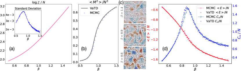
Figure 2: (a) The estimated free energy and its standard deviation (inset) of the 2D XY model on a $16\times 16$ PBC square lattice. The temperature factor (-$T$) is removed for better comparison. (b) The estimated square magnetization of the XY model. (c) Configurations directly sampled from the learned model at three temperatures, the background color represents the vorticity. (d) The mean energy and heat capacity of the XY model, estimated using the differentiation of the free energy, compared with the results obtained from the MCMC simulation.

The XY model is more complex than the Ising model. As an example of the BKT transition [27, 28], the XY model finds practical applications in explaining various systems, including thin ${}^{4}\mathrm{He}$ films [29], and quasi-2D layered superconductors [30]. The energy function of the XY model is $E(\mathbf{x})=-\sum_{<i,j>}\cos(x_{i}-x_{j})$, where $x_{i}$ and $x_{j}$ are angles in the continuous range of $[-\pi,\pi]$. Similar to the Ising case, we also used a 2D $16\times 16$ square lattice with PBC for the XY model.

We chose NF models for continuous variables in a closed range [31, 32, 33, 34, 35]. In a NF model, the samples are initially drawn from a prior distribution, which is easy to sample from. We chose the von Mises distribution ,$\text{VM}(\mu,\kappa)$ where $\mu$ controls the mean and $\kappa$ controls the variance [36, 37], as the prior distribution of angles. To have a temperature-differentiable prior distribution, we modified $\kappa$ as $\kappa_{\beta}=\kappa\cdot\beta$. As VMs are sampled by an acceptance-rejection method, a special reparameterization should be used to optimize the $\mu$ and $\kappa$ [38, 17] (see the appendix). The sample $\bm{z}$ from the VM prior distribution was then transformed using parameterized invertible transformations, i.e., $\bm{x}=f_{\theta}(\bm{z},\beta)$. To incorporate temperature, we again repeated $\beta$ and padded it with the sample variables in the channel dimension, which is similar to the Ising case. The effects of these invertible transformations, besides changing the sample variables, also introduce probability changes to the VM prior distribution. These distribution changes are measured by the determinant of the Jacobian matrices [31]. The invertible transformation we chose is the piece-wise cubic spline transformation [35]. This kind of transformation is designed for continuous variables in a closed range. Then, the final probability of a sample is the product of the prior probability and the determinant of the Jacobian, $q_{\theta}(\mathbf{x},\beta)=\text{VM}(\bm{z}|\mu,\kappa_{\beta})\cdot|\text{det}\frac{\partial\bm{z}}{\partial\mathbf{x}}|$. This model was trained in the temperature range of $\beta\in[0.4,2.0]$. The $O(1)$ symmetry was eliminated by pinning the first spin to $0$.

After training, we performed direct sampling and used the obtained batches to perform statistical averaging. Fig. 2(a) shows the estimated free energy as a continuous function of temperature. As XY is not exactly solvable, we calculated the standard deviation (STD) to evaluate the estimation quality. According to Eq. (4), a perfect model would produce uniform estimates regardless of $\bm{x}$, so the small STDs in Fig. 2(a) indicate very good simulation results. Fig. 2(b) shows the estimated square magnetization, in excellent agreement with the MCMC result. To study the microscopic behavior, we plotted the sampled configurations at different temperatures in Fig. 2(c), which clearly shows the microscopic changes occurring near the PT. Specifically, with decreasing temperature, the vortex density decreases, and a quasi long-range order emerges. This demonstrates a good capture of the underlying physical transition.

Furthermore, we compared the mean energy and heat capacity obtained by the MCMC simulation and the differentiation of the free energy in Fig. 2(d). In comparison to the MCMC result, we observed only minor deviations in the heat capacity around the PT, indicating a good fit of the free energy to the second-order derivative and a good capture of the subtle PT transition. Numerical results in appendix also show that the derivative estimation gives better convergence than the statistical averaging [17]. In contrast to the one-by-one generation process of PixelCNN, the NF model is significantly faster due to its all-to-all style of generation. This leads to a comparable training-plus-evaluation time (36 hours on one Nvidia RTX 4090) to performing an MCMC sweep over many temperature points. Additionally, the low STD allows us to estimate the heat capacity using the first-order derivative, which offers a significant speed-up and reduces the memory requirement. We give a detailed description of this scheme in appendix [17].

Outlooks.

In this Letter, we present a novel framework of variational training for the explicit density generative models. By converting the Boltzmann distribution optimization problem into a temperature-dependent loss function, we achieve a direct-sampling Boltzmann distribution model with explicit temperature dependence. This allows thermodynamic quantities, such as free energy and partition function, to be differentiable functions of temperature. Our proposed method is as accurate as the MCMC method, but more efficient due to direct sampling. Moreover, as a single model with temperature dependence, its direct-sampling estimation remains valid across a continuous temperature range. In contrast to previous deep generative models that optimize at a single temperature, our method preserves the essential temperature dependence akin to an analytical solution. As a result, there is no need for training additional models at discrete temperature points, and a single model can reliably capture subtle thermal effects, even at PTs.

With minor modifications, we expect to have immediate practical applications by adapting our method to these popular deep generative variational models of single temperature [12, 13, 14, 15, 39, 40, 16]. Our proposed method can be seen as a generalization of the variational mean-field method, which consists of multiple conditional parameters. While our current method focuses on temperature, it opens up intriguing possibilities for exploring other parameters, such as the pressure and external magnetization fields. Here we mainly applied our method to lattice models, but it is also viable to extend its application to more realistic systems with many meta-stable states, e.g., atomisitic simulations.

Supplemental Information: Deep generative modelling of canonical ensemble with differentiable thermal properties

Appendix A Variational Minimization of the Free Energy

Given a probability distribution $q(\mathbf{x})$ and an energy function $E(\mathbf{x})$, the free energy is

$$F=TS+\langle E\rangle=\sum_{\{\mathbf{x}\}}\frac{1}{\beta}q(\mathbf{x})\log q(\mathbf{x})+q(\mathbf{x})E(\mathbf{x}).$$ (S1)

As a probability distribution, $q(\mathbf{x})$ has the following constraint,

$$\sum_{\{\mathbf{x}\}}q(\mathbf{x})=1.$$ (S2)

Considering a $q^{*}$ that minimizes the free energy for all temperatures, then this $q^{*}$ should be the solution to the following optimization problem.

$$\min_{q(\mathbf{x})}{} \frac{1}{\beta}\Big{[}\sum_{\{\mathbf{x}\}}q(\mathbf{x})\log q(\mathbf{x})+\beta q(\mathbf{x})E(\mathbf{x})\Big{]},$$ (S3)

s.t. $$~{}\sum_{\{\mathbf{x}\}}q(\mathbf{x})=1,~{}\forall\beta.$$

This optimization can be analytically solved via the Lagrange multiplier method [41], which gives the Boltzmann distribution as a function of temperature, i.e.,

$${q}^{*}(\mathbf{x})=\frac{\exp(-\beta E(\mathbf{x}))}{\sum_{\{\mathbf{x}\}}\exp(-\beta E(\mathbf{x}))}=\frac{\exp(-\beta E(\mathbf{x}))}{\mathcal{Z}}.$$ (S4)

To solve this in a variational way, we use a variational model $q_{\theta}$. Then, because the requirement of the minimum at every $\beta$ point implies the minimum of an integration over all $\beta$ points, we can turn Eq. (S3) into

$$\min_{\theta}\int \frac{1}{\beta}\Big{[}\sum_{\{\mathbf{x}\}}q_{\theta}(\mathbf{x})\log q_{\theta}(\mathbf{x})+\beta q_{\theta}(\mathbf{x})E(\mathbf{x})\Big{]}d\beta,$$ (S5)

s.t. $$~{}\sum_{\{\mathbf{x}\}}q(\mathbf{x})=1.$$

This can also be interpreted as an integration over an equal-probability distribution of $\beta$, which can be estimated via a uniform sampling, i.e.,

$$\min_{\theta}\mathop{\mathbb{E}}_{\beta\sim U} \frac{1}{\beta}\Big{[}\sum_{\{\mathbf{x}\}}q_{\theta}(\mathbf{x})\log q_{\theta}(\mathbf{x})+\beta q_{\theta}(\mathbf{x})E(\mathbf{x})\Big{]},$$ (S6)

s.t. $$~{}\sum_{\{\mathbf{x}\}}q(\mathbf{x})=1.$$

Using an explicit density model, one can directly sample $\bm{x}$ to perform statistical averaging as an estimation of the summation over $\{\bm{x}\}$, and the probability normalization condition is automatically satisfied, so we get

$$\min_{\theta}\mathop{\mathbb{E}}_{\beta\sim U}\frac{1}{\beta}\Big{[}\mathop{\mathbb{E}}_{\bm{x}\sim q_{\theta}(\cdot,\beta)}q_{\theta}(\mathbf{x})\log q_{\theta}(\mathbf{x})+\beta q_{\theta}(\mathbf{x})E(\mathbf{x})\Big{]},$$ (S7)

which is the Eq. (6) in the main text.

Appendix B Reparameterization and Reinforce Estimation

B.1 First-order and second-order reparameterization

The reparameterization introduces a new random variable $\epsilon$ and rewrites the original expectation into an expectation over the distribution of $\epsilon$, i.e.,

$$\mathop{\mathbb{E}}_{\mathbf{x}\sim q_{\theta}(\mathbf{x})}f(\mathbf{x};\theta)=\mathop{\mathbb{E}}_{\epsilon\sim\pi(\epsilon)}f(h_{\theta}(\epsilon);\theta),~{}\mathbf{x}=h_{\theta}(\epsilon).$$ (S8)

The derivatives can be reformulated as

$$\begin{split}\nabla_{\theta}\mathop{\mathbb{E}}_{\mathbf{x}\sim q_{\theta}(\mathbf{x})}f(\mathbf{x};\theta)=&\nabla_{\theta}\mathop{\mathbb{E}}_{\epsilon\sim\pi(\epsilon)}f(h_{\theta}(\epsilon);\theta)\\ =&\mathop{\mathbb{E}}_{\epsilon\sim\pi(\epsilon)}\nabla_{\theta}f(h_{\theta}(\epsilon);\theta),\\ \nabla^{2}_{\theta}\mathop{\mathbb{E}}_{\mathbf{x}\sim q_{\theta}(\mathbf{x})}f(\mathbf{x};\theta)=&\nabla^{2}_{\theta}\mathop{\mathbb{E}}_{\epsilon\sim\pi(\epsilon)}f(h_{\theta}(\epsilon);\theta)\\ =&\mathop{\mathbb{E}}_{\epsilon\sim\pi(\epsilon)}\nabla^{2}_{\theta}f(h_{\theta}(\epsilon);\theta).\end{split}$$ (S9)

B.2 First-order and second-order reinforce estimation

The reinforce estimation utilizes the log-derivative trick which is

$$\nabla_{\theta}q_{\theta}(\mathbf{x})=q_{\theta}(\mathbf{x})\nabla_{\theta}\log q_{\theta}(\mathbf{x}).$$ (S10)

The first-order derivative is

$$\begin{split}&\nabla_{\theta}\mathop{\mathbb{E}}_{\mathbf{x}\sim q_{\theta}(\mathbf{x})}f(\mathbf{x};\theta)=\nabla_{\theta}\sum_{\{\mathbf{x}\}}q_{\theta}(\mathbf{x})f(\mathbf{x};\theta)\\ =&\sum_{\{\mathbf{x}\}}\left[f(\mathbf{x};\theta)q_{\theta}(\mathbf{x})\nabla_{\theta}\log q_{\theta}(\mathbf{x})+q_{\theta}(\mathbf{x})\nabla_{\theta}f(\mathbf{x};\theta)\right]\\ =&\mathop{\mathbb{E}}_{\mathbf{x}\sim q_{\theta}(\mathbf{x})}\left[f(\mathbf{x};\theta)\nabla_{\theta}\log q_{\theta}(\mathbf{x})+\nabla_{\theta}f(\mathbf{x};\theta)\right].\end{split}$$ (S11)

Note that

$$\mathop{\mathbb{E}}_{\mathbf{x}\sim q_{\theta}(\mathbf{x})}\nabla_{\theta}\log q_{\theta}(\mathbf{x})=\nabla_{\theta}\sum_{\{\mathbf{x}\}}q_{\theta}(\mathbf{x})=\nabla_{\theta}1=0.$$ (S12)

The variance of estimate of Eq. (S11) can be reduced via [23]

$$\nabla_{\theta}\mathop{\mathbb{E}}_{\mathbf{x}\sim q_{\theta}(\mathbf{x})}f(\mathbf{x};\theta)$$ (S13)

$$= \mathop{\mathbb{E}}_{\mathbf{x}\sim q_{\theta}(\mathbf{x})}\left[(f(\mathbf{x};\theta)-b)\nabla_{\theta}\log q_{\theta}(\mathbf{x})+\nabla_{\theta}f(\mathbf{x};\theta)\right],$$

where $b$ is the baseline. $b$ has many different forms [23] and here we use the simplest one:

$$b=\mathop{\mathbb{E}}_{\mathbf{x}\sim q_{\theta}(\mathbf{x})}f(\mathbf{x};\theta).$$ (S14)

The second-order derivative is

$$\nabla^{2}_{\theta}\mathop{\mathbb{E}}_{\mathbf{x}\sim q_{\theta}(\mathbf{x})}f(\mathbf{x};\theta)$$ (S15)

$$= \nabla_{\theta}\sum_{\{\mathbf{x}\}}f(\mathbf{x};\theta)q_{\theta}(\mathbf{x})\nabla_{\theta}\log q_{\theta}(\mathbf{x})+q_{\theta}(\mathbf{x})\nabla_{\theta}f(\mathbf{x};\theta)$$

$$= \sum_{\{\mathbf{x}\}}f(\mathbf{x};\theta)q_{\theta}(\mathbf{x})\nabla^{2}_{\theta}\log q_{\theta}(\mathbf{x})+f(\mathbf{x};\theta)q_{\theta}(\mathbf{x})(\nabla_{\theta}\log q_{\theta}(\mathbf{x}))^{2}$$

$$+\sum_{\{\mathbf{x}\}}q_{\theta}(\mathbf{x})\nabla_{\theta}^{2}f(\mathbf{x};\theta)+2\nabla_{\theta}f(\mathbf{x};\theta)q_{\theta}(\mathbf{x})\nabla_{\theta}\log q_{\theta}(\mathbf{x})$$

$$= \mathop{\mathbb{E}}_{\mathbf{x}\sim q_{\theta}(\mathbf{x})}\Big{[}f(\mathbf{x};\theta)\left(\nabla^{2}_{\theta}\log q_{\theta}(\mathbf{x})+\left(\nabla_{\theta}\log q_{\theta}(\mathbf{x})\right)^{2}\right)\Big{]}$$

$$+\mathop{\mathbb{E}}_{\mathbf{x}\sim q_{\theta}(\mathbf{x})}\Big{[}\nabla_{\theta}^{2}f(\mathbf{x};\theta)+2\nabla_{\theta}f(\mathbf{x};\theta)\nabla_{\theta}\log q_{\theta}(\mathbf{x})\Big{]}.$$

Note that

$$\mathop{\mathbb{E}}_{\mathbf{x}\sim q_{\theta}(\mathbf{x})}\left[\nabla^{2}_{\theta}\log q_{\theta}(\mathbf{x})+(\nabla_{\theta}\log q_{\theta}(\mathbf{x}))^{2}\right]$$ (S16)

$$=\nabla_{\theta}^{2}\sum_{\{\mathbf{x}\}}q_{\theta}(\mathbf{x})=0.$$

The variance reduction method can be also employed

$$\nabla^{2}_{\theta}\mathop{\mathbb{E}}_{\mathbf{x}\sim q_{\theta}(\mathbf{x})}f(\mathbf{x};\theta)$$ (S17)

$$= \mathop{\mathbb{E}}_{\mathbf{x}\sim q_{\theta}(\mathbf{x})}\Big{[}(f(\mathbf{x};\theta)-b_{1})\left(\nabla^{2}_{\theta}\log q_{\theta}(\mathbf{x})+\left(\nabla_{\theta}\log q_{\theta}(\mathbf{x})\right)^{2}\right)\Big{]}$$

$$+\mathop{\mathbb{E}}_{\mathbf{x}\sim q_{\theta}(\mathbf{x})}\Big{[}\nabla_{\theta}^{2}f(\mathbf{x};\theta)+2\left(\nabla_{\theta}f(\mathbf{x};\theta)-b_{2}\right)\nabla_{\theta}\log q_{\theta}(\mathbf{x})\Big{]},$$

where

$$\begin{split}b_{1}=&\mathop{\mathbb{E}}_{\mathbf{x}\sim q_{\theta}(\mathbf{x})}f(\mathbf{x};\theta),\\ b_{2}=&\mathop{\mathbb{E}}_{\mathbf{x}\sim q_{\theta}(\mathbf{x})}\nabla_{\theta}f(\mathbf{x};\theta).\end{split}$$ (S18)

B.3 Reparameterization of acceptance-rejection sampling

The acceptance-rejection sampling is a common way to draw samples from certain relatively complex distributions. The reparameterization of acceptance-rejection sampling is given in Ref. [38]. For a better illustration, we first give the general framework of acceptance-rejection sampling.

In acceptance-rejection sampling, to sample distribution $q_{\theta}(z)$, we first draw a random variable $\epsilon$ from the distribution $s(\epsilon)$. It is then transformed using a parameterized transformation $h_{\theta}$, similar to the NF case, we should consider the Jacobian of the transformation. Then its possibility changes to $r_{\theta}({z})$, where ${z}=h_{\theta}(\epsilon)$. One accepts the sample with the probability $\min\{1,\frac{q_{\theta}({z})}{M_{\theta}r_{\theta}({z})}\}$ or rejects it, as in Alg. 1.

Input : $s$, $h_{\theta}$, $M_{\theta}$, and $q_{\theta}$

Output : ${z}=h_{\theta}(\epsilon)$

1 $i\leftarrow 0$;

2 repeat

3       $i\leftarrow i+1$;

4       $\epsilon\sim s(\epsilon),{z}=h_{\theta}(\epsilon)$;

5       $u\sim{U}(0,1)$;

6      

7until $u<\frac{q_{\theta}({z})}{M_{\theta}r_{\theta}({z})}$;

return ${z}$

Algorithm 1 acceptance-rejection sampling

The probability distribution of the accepted $\epsilon$ is

$$\pi_{\theta}(\epsilon)= \int M_{\theta}s(\epsilon)\mathds{1}\left(0<u<\frac{q_{\theta}(h_{\theta}(\epsilon))}{M_{\theta}r(h_{\theta}(\epsilon);\theta)}\right)du$$ (S19)

$$= s(\epsilon)\frac{q_{\theta}(h_{\theta}(\epsilon))}{r(h_{\theta}(\epsilon);\theta)}.$$

The first-order derivative can be reformulated as

$$\nabla_{\theta}\mathop{\mathbb{E}}_{{z}\sim q_{\theta}({z})}f({z};{\theta})=\nabla_{\theta}\mathop{\mathbb{E}}_{\epsilon\sim\pi_{\theta}(\epsilon)}f(h_{\theta}(\epsilon);\theta).$$ (S20)

Then, using the log-derivative trick, this becomes

$$\mathop{\mathbb{E}}_{\epsilon\sim s(\epsilon)}\left[\frac{q_{\theta}(h_{\theta}(\epsilon))}{r(h_{\theta}(\epsilon);\theta)}\nabla_{\theta}f(h_{\theta}(\epsilon);\theta)\right]+\mathop{\mathbb{E}}_{\epsilon\sim s(\epsilon)}\left[\frac{q_{\theta}(h_{\theta}(\epsilon))}{r(h_{\theta}(\epsilon);\theta)}f(h_{\theta}(\epsilon);\theta)\nabla_{\theta}\log\frac{q_{\theta}(h_{\theta}(\epsilon))}{r(h_{\theta}(\epsilon);\theta)}\right].$$ (S21)

We generalize the scheme in [38], and give the second-order derivative

$$\nabla_{\theta}^{2}\mathop{\mathbb{E}}_{{z}\sim q_{\theta}({z})}f({z};{\theta})=\nabla_{\theta}^{2}\mathop{\mathbb{E}}_{\epsilon\sim\pi_{\theta}(\epsilon)}f(h_{\theta}(\epsilon);\theta).$$ (S22)

This is

$$\nabla_{\theta}\int s(\epsilon)\frac{q_{\theta}(h_{\theta}(\epsilon))}{r(h_{\theta}(\epsilon);\theta)}\nabla_{\theta}f(h_{\theta}(\epsilon);\theta)d\epsilon$$ (S23)

$$+\nabla_{\theta}\int s(\epsilon)f(h_{\theta}(\epsilon);\theta)\nabla_{\theta}\frac{q_{\theta}(h_{\theta}(\epsilon))}{r(h_{\theta}(\epsilon);\theta)}d\epsilon$$

$$= 2\mathop{\mathbb{E}}_{\epsilon\sim s(\epsilon)}\left[\frac{q_{\theta}(h_{\theta}(\epsilon))}{r(h_{\theta}(\epsilon);\theta)}\nabla_{\theta}f(h_{\theta}(\epsilon);\theta)\nabla_{\theta}\log\frac{q_{\theta}(h_{\theta}(\epsilon))}{r(h_{\theta}(\epsilon);\theta)}\right]$$

$$+\mathop{\mathbb{E}}_{\epsilon\sim s(\epsilon)}\left[\frac{q_{\theta}(h_{\theta}(\epsilon))}{r(h_{\theta}(\epsilon);\theta)}\nabla_{\theta}^{2}f(h_{\theta}(\epsilon);\theta)\right]$$

$$+\mathop{\mathbb{E}}_{\epsilon\sim s(\epsilon)}\left[f(h_{\theta}(\epsilon);\theta)\nabla_{\theta}^{2}\frac{q_{\theta}(h_{\theta}(\epsilon))}{r(h_{\theta}(\epsilon);\theta)}\right].$$

Note that

$$\mathop{\mathbb{E}}_{\epsilon\sim s(\epsilon)}\nabla_{\theta}\frac{q_{\theta}(h_{\theta}(\epsilon))}{r(h_{\theta}(\epsilon);\theta)}=\int\nabla_{\theta}\pi_{\theta}(\epsilon)d\epsilon=0,$$ (S24)

$$\mathop{\mathbb{E}}_{\epsilon\sim s(\epsilon)}\nabla_{\theta}^{2}\frac{q_{\theta}(h_{\theta}(\epsilon))}{r(h_{\theta}(\epsilon);\theta)}=\int\nabla_{\theta}^{2}\pi_{\theta}(\epsilon)d\epsilon=0,$$

so the variance reduction method [23] can also be applied here.

For the von Mises distribution $\text{VM}(\mu,\kappa)$, the $s$ distribution is

$$\epsilon_{1},\epsilon_{2}\sim\text{U}(0,1).$$ (S25)

The transformation $h_{\theta}$ is

$$h_{\theta}(\epsilon_{1},\epsilon_{2})=\text{sign}(\epsilon_{2}-0.5)\cos^{-1}\left(\frac{1+cz}{c+z}\right)+\mu,$$ (S26)

where

$$b=1+\sqrt{1+4\kappa^{2}},$$ (S27)

$$\rho=(b-\sqrt{2b})/2\kappa,$$

$$c=(1+\rho^{2})/(2\rho),$$

$$z=\cos(\pi\epsilon_{1}).$$

Similar to the NF model case, the $r_{\theta}$ distribution can be derived using the $s$ distribution and the Jacobian of $h_{\theta}$.

Appendix C Macroscopic Behaviors from the Differentiation of the Free Energy

C.1 Analysis of the differentiation method compared to the statistical averaging with direct sampling

After training a direct-sample model with differentiable temperature condition, to estimate mean energy and heat capacity, other than the differentiation method in Eq. (2), one can also perform statistical averaging with direct sampling, i.e.,

$$\langle E\rangle=\mathop{\mathbb{E}}_{\mathbf{x}\sim q_{\theta}}E(\mathbf{x}),~{}C_{v}=\beta^{2}(\mathop{\mathbb{E}}_{\mathbf{x}\sim q_{\theta}}E^{2}(\bm{x})-(\mathop{\mathbb{E}}_{\mathbf{x}\sim q_{\theta}}E(\bm{x}))^{2}).$$ (S28)

For a better analysis, We establish a connection between the two methods.

Using Eq. (2), given the estimated $-\log\bar{\mathcal{Z}}(\beta)$, the mean energy is

$$\langle E\rangle= -\frac{\partial\log\bar{\mathcal{Z}}(\beta)}{\partial\beta}$$ (S29)

$$= \frac{\partial}{\partial\beta}\sum_{\mathbf{x}}q_{\theta}(\mathbf{x},\beta)\left[\log q_{\theta}(\mathbf{x},\beta)+\beta E(\mathbf{x})\right]$$

$$= \sum_{\mathbf{x}}q_{\theta}(\mathbf{x},\beta)\left[\log q_{\theta}(\mathbf{x},\beta)+\beta E(\mathbf{x})\right]\frac{\partial\log q_{\theta}(\mathbf{x},\beta)}{\partial\beta}$$

$$+\sum_{\mathbf{x}}q_{\theta}(\mathbf{x},\beta)E(\mathbf{x}).$$

It can be seen that if the learned distribution is the exact Boltzmann distribution, i.e.,

$$q_{\theta}(\mathbf{x},\beta)\vcentcolon=\frac{\exp(-\beta E(\mathbf{x}))}{\mathcal{Z}},$$ (S30)

Eq. (S29) becomes

$$\langle E\rangle=\mathop{\mathbb{E}}_{\mathbf{x}\sim q_{\theta}(\mathbf{x},\beta)}E(\mathbf{x}).$$ (S31)

A similar analysis can be done for the heat capacity with the same conclusion; that is, when the training is perfectly done, the differentiation method gives the same results as direct sampling. However, for imperfect training, the two methods give different results. The differentiation results, as they’re closely related to the minimization goal, have a better accuracy than the statistical average. Additionally, one can view the VaTD training as a generalization of the variational mean-field method. In the mean-field theory, when the variational ansatz $q_{\theta}$ is not flexible enough, the $q_{\theta}$ may not converge to the target distribution $p$, but still could have a relative accurate estimation of the partition function (or free energy).

On the other hand, even with perfect or near-perfect training, it is better to choose the differentiation method, because the differentiation method has a much faster convergence speed. From Eq. (4), one can see that a perfect model will give uniformly the same estimate of the free energy for any $\bm{x}$. In this sense, a batch of just one sample will converge.

The numerical tests in the following sections demonstrate these two advantages of the differentiation method.

C.2 Estimation of the heat capacity using first-order differentiation

As the second-order derivatives are not memory-efficient for backpropagation automatic differentiation, we propose a scheme to estimate the heat capacity using the first-order differentiation when the loss of the model is low enough.

Consider the first-order differentiation

$$\frac{\partial}{\partial\beta}\sum_{\{\mathbf{x}\}}q_{\theta}(\mathbf{x},\beta)\log q_{\theta}(\mathbf{x},\beta)$$ (S32)

$$= \sum_{\{\mathbf{x}\}}\frac{\partial q_{\beta}(\mathbf{x},\beta)}{\partial\beta}\log q_{\theta}(\mathbf{x},\beta)+\frac{\partial q_{\theta}(\mathbf{x},\beta)}{\partial\beta}$$

$$= \sum_{\{\mathbf{x}\}}\frac{\partial q_{\theta}(\mathbf{x},\beta)}{\partial\beta}\log q_{\theta}(\mathbf{x},\beta),$$

where $q_{\theta}(\mathbf{x},\beta)$ is the distributino of the VaTD model. When the loss is low enough, we assume the distribution of VaTD has the form of the Boltzmann distribution, i.e.,

$$q_{\theta}(\mathbf{x},\beta)\vcentcolon=\frac{\exp(-\beta E_{\theta}(\mathbf{x}))}{\bar{\mathcal{Z}}},$$ (S33)

where $E_{\theta}$ is the energy function learned by the VaTD. Then, Eq. (S32) can be reformulated into

$$\sum_{\{\mathbf{x}\}}q_{\theta}(\mathbf{x},\beta)\left(-E_{\theta}(\mathbf{x})-\frac{\partial\log\bar{\mathcal{Z}}}{\partial\beta}\right)(-\beta E_{\theta}(\mathbf{x},\beta)-\log\bar{\mathcal{Z}})$$ (S34)

$$= \sum_{\{\mathbf{x}\}}q_{\theta}(\mathbf{x},\beta)(E_{\theta}(\mathbf{x})-\langle E_{\theta}\rangle)(\beta E_{\theta}(\mathbf{x},\beta)+\log\bar{\mathcal{Z}})$$

$$= \sum_{\{\mathbf{x}\}}\left[q_{\theta}(\mathbf{x},\beta)(E_{\theta}(\mathbf{x})-\langle E_{\theta}\rangle)\log\bar{\mathcal{Z}}\right]+\beta(\langle E^{2}_{\theta}\rangle-\langle E_{\theta}\rangle^{2}).$$

From Eq. (4), when the model is trained to be a Boltzmann distribution, $\log\bar{\mathcal{Z}}$ is a constant for any $\bm{x}$. In that case, the former term in Eq. (S34) disappears, and the latter is related to the heat capacity, so the heat capacity can be written as

$$C_{v}=\beta\frac{\partial}{\partial\beta}\left[\mathop{\mathbb{E}}_{\mathbf{x}\sim q_{\theta}(\cdot,\beta)}\log q_{\theta}(\mathbf{x},\beta)\right]\approx\beta^{2}(\langle E^{2}_{\theta}\rangle-\langle E_{\theta}\rangle^{2}).$$ (S35)

Appendix D Supplementary for the 2D Ising Model Experiment

D.1 Architecture and hyperparameters

The architecture we used is a standard ResNet [25] structure with the CNN layer replaced by the masked CNN layer of [24]. For training, we used the Adam optimizer [42], whose learning rate was reduced periodically. Because the reinforce estimation tends to have high variance, we clipped the gradient values that are greater than a maximum value. All structural and training parameters can be found in Tab. S1. Except for the configuration plots, all the results showed in the Ising model simulation in the main text are estimated using a batch size of $7000$.

Table S1: Hyperparameters of the PixelCNN model used in the 2D Ising model experiment.

Structural parameter
ResNet kernel size	13
ResNet channel	64
ResNet block	6
Fully-connected CNN layer	2
Activation function	RELU [44]
Training parameter
Batch size	500
Learning rate	$5\times 10^{-4}$
Decay factor	0.92
Gradient clip	1.0
Betas	(0.9, 0.999)
Eps	$10^{-8}$

D.2 Statistical averages with direct sampling

In this section, we compared the numerical results from the differentiation of the free energy with those from the statistical averaging with direct sampling. As the model in Fig. 1 of the main text has a too-low loss value, one may think the condition of Eq. (S30) is nearly satisfied, so a clear difference is not visible. To better illustrate it numerically, we used a saved model near the end of the training which has a slightly higher loss value.

In Fig. S1, using this secondary model, we plotted the heat capacity values of the 2D Ising model using automatic differentiation and statisitcal averaging with direct sampling. Compared with the automatic differentiation results, statistical averages show a larger deviation. In this plot, a batch of $7000$ samples was generated by the model at each temperature point.

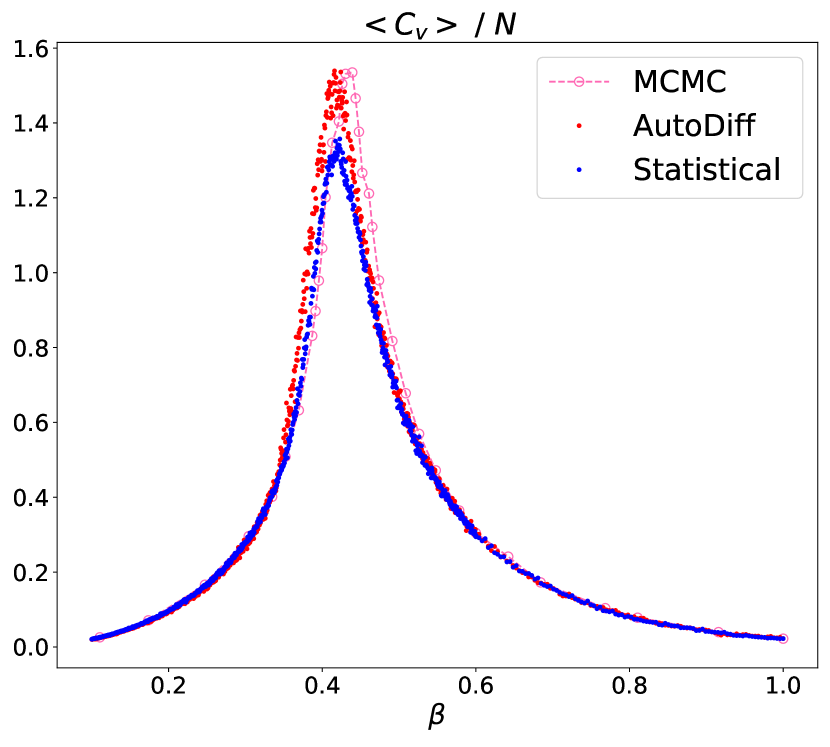
Figure S1: The estimated heat capacity of the 2D Ising model on a $16\times 16$ PBC square lattice. The estimation results using differentiation of free energy (labeled as autoDiff) and statistical averaging with direct sampling (labeled as statistical) are compared with the MCMC results.

Appendix E Supplementary for the 2D XY Model Experiment

E.1 Architecture and hyperparameters

Our architecture consists of multiple layers of the piece-wise cubic spline transformation flow [35]. The cubic spline transformation uses interpolation points to create a monotonically increasing function to parameterize the invertible transformation. The coordinates and gradients of these interpolation points were computed using a standard ResNet [25]. The cubic spline flow also needs a way to bisect the variables. As the 2D XY configuration is a 2D array, we used the checkerboard pattern to separate it into two parts with an equal amount of variables. For training, we used the Adam optimizer [42], and we decreased the learning rate periodically. All structural and training parameters can be found in Tab. S2. Except for the configuration plots, all the results showed in the XY model experiment of the main text were estimated using a batch size of $1000$.

Table S2: Hyperparameters of the NF model used in the 2D XY model experiment.

Structural parameter
Cubic transformation layer	5
Interpolation point number	45
ResNet kernel size	9
ResNet channel	128
ResNet block	6
Fully-connected CNN layer	2
Activation function	ELU [43]
Training parameter
Batch size	1024
Learning rate	$7\times 10^{-4}$
Decay factor	0.7
Decay step	1000
Betas	(0.9, 0.999)
Eps	$10^{-8}$

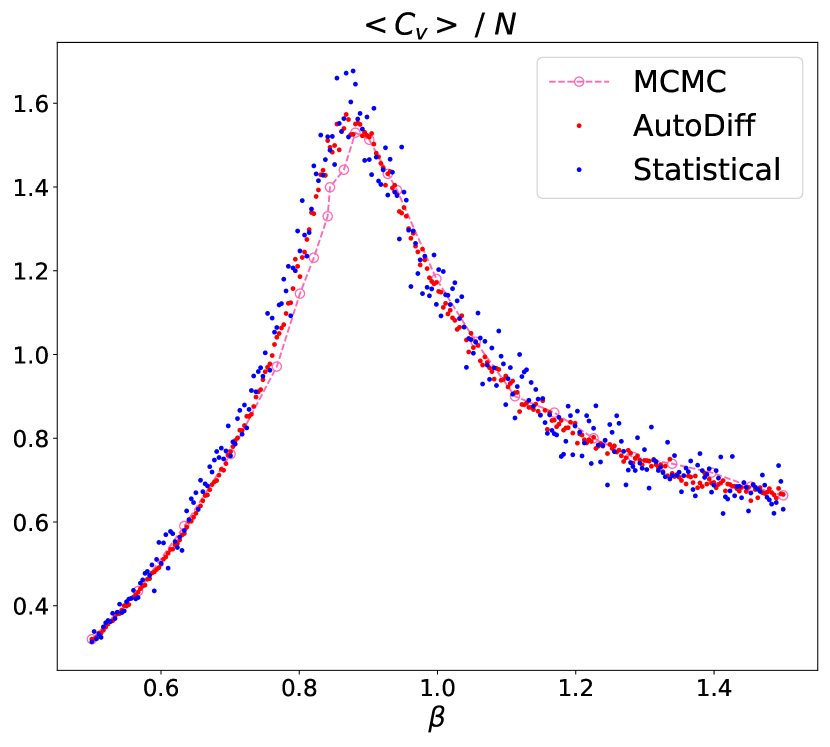
Figure S2: The estimated heat capacity of the 2D XY model on a $16\times 16$ PBC square lattice. The estimation results using differentiation of free energy (labeled as autoDiff) and statistical averaging with direct sampling (labeled as statistical) are compared with the MCMC results.

E.2 Statistical averages with direct sampling

Using this XY case, we further demonstrated numerically the difference between automatic differentiation and direct sampling. In Fig. S2, we gave the statistical averaging results of the heat capacity compared with differentiation results. In this plot, a batch of $1000$ samples was directly sampled by the model at each temperature point, for both the statistical averages and differentiation results. One can see that the statistical averages have a larger variance using the same number of samples.