The defect $b$-theorem under bulk RG flows

Abstract

It is known that for RG flows confined to a two-dimensional defect, where the bulk maintains its conformal nature, the coefficient of the Euler density in the defect’s Weyl anomaly (termed $b$) cannot increase as the flow progresses from the ultraviolet to the infrared, a principle known as the $b$-theorem. In this paper, we investigate whether this theorem still holds when the bulk, instead of being critical, also undergoes an RG flow. To address this question, we examine two distinct and perturbatively tractable examples. Our analysis reveals that a straightforward extension of the $b$-theorem to these cases of RG flows fails.

1 Introduction

The renormalization group (RG) flow serves as a foundational framework for identifying the degrees of freedom governing low-energy phenomena. Its core premise lies in simplifying theories by disregarding their microscopic details while preserving their low-energy physics. This simplification inevitably reduces the number of degrees of freedom, sparking a longstanding debate regarding the quantification of this reduction. Zamolodchikov’s c-theorem Zamolodchikov:1986gt provided the first precise quantification of this kind for a broad class of two-dimensional quantum field theories, catalyzing numerous advancements across various spacetime dimensions and expanding our understanding of RG flows and their implications.

Extending Zamolodchikov’s theorem to higher dimensions, let alone to the case of QFTs with defects, has proven to be a challenging endeavour, leading to ongoing research efforts aimed at elucidating the nature of RG flows beyond the two-dimensional case Cardy:1988cwa ; Cappelli:1990yc ; Osborn:1991gm ; Myers:2010tj ; Jafferis:2011zi ; Komargodski:2011vj ; Komargodski:2011xv ; Casini:2012ei ; Elvang:2012st ; Yonekura:2012kb ; Grinstein:2013cka ; Jack:2013sha ; Giombi:2014xxa ; Jack:2015tka ; Cordova:2015fha ; Casini:2015woa ; Casini:2017vbe ; Fluder:2020pym ; Delacretaz:2021ufg .

In this paper, we delve into the study of RG flows in the presence of two-dimensional defects. Our focus lies exclusively on scenarios where the bulk QFT is a $d$-dimensional Euclidean field theory, with the state being the flat space vacuum state. In such configurations, both the defect and the bulk can undergo RG flows, thereby rendering existing analogs of the c-theorem inapplicable. Despite the extensive history of defects in both two and higher dimensions Cardy:1984bb ; Cardy:1989ir ; McAvity:1995zd ; Affleck:1995ge ; Sachdev99 ; Vojta_2000 ; Polchinski:2011im ; Gaiotto:2013nva ; Billo:2016cpy ; Bianchi:2015liz ; Solodukhin:2015eca ; Fursaev:2016inw ; Lauria:2018klo ; Gadde:2016fbj ; Herzog:2020bqw ; Giombi:2021uae ; Liu_2021 ; Herzog:2022jqv , a robust candidate to quantify the reduction of degrees of freedom when both the bulk and the defect undergo simultaneous RG flows remains elusive and rarely addressed.

In contrast, defect RG flows with fixed conformal bulk, also known as DRG in the literature, have undergone extensive studies Affleck:1991tk ; Yamaguchi:2002pa ; Azeyanagi:2007qj ; Estes:2014hka ; Andrei:2018die ; Kobayashi:2018lil ; Casini:2018nym ; Lauria:2020emq ; Giombi:2020rmc ; Wang:2020xkc ; Nishioka:2021uef ; Sato:2021eqo ; CarrenoBolla:2023vrv . Numerous exact results regarding RG flows on line defects Friedan:2003yc ; Casini:2016fgb ; Cuomo:2021rkm ; Casini:2022bsu and their higher-dimensional generalizations Jensen:2015swa ; Wang:2021mdq ; Shachar:2022fqk have been established. In particular, the so-called $b$-theorem Jensen:2015swa ; Shachar:2022fqk asserts that the dimensionless ”central charge,” which multiplies the Euler density in the defect’s Weyl anomaly, necessarily decreases or remains constant along the DRG flow from the UV to an IR fixed point, providing a quantitative diagnostic for the irreversibility of the DRG flows on two-dimensional defects.

In this work, we pose a natural question: does the $b$-theorem still hold if the condition of a conformal bulk is relaxed, subjecting it to changes under an RG flow? We term this version of the $b$-theorem a naive generalization, and proceed to test it in two specific examples in $4-\epsilon$ dimensions: the $O(N)$ vector model and the Gross-Neveu-Yukawa model. Our calculations illustrate that when the flow extends beyond the defect, implying that the bulk is not conformally invariant and undergoes changes along the RG flow, the naive extension of the $b$-theorem is compromised.

The paper is organized as follows: in Section 2, we employ conformal perturbation theory to derive perturbative beta functions for a generic CFT deformed by a set of relevant operators in the bulk and on the two-dimensional defect. Sections 3 and 4 are dedicated to scrutinizing RG flows in the presence of defects, using two examples of QFTs in $4-\epsilon$ dimensions that are perturbatively tractable: the $O(N)$ vector model and the Gross-Neveu-Yukawa model. We conclude with a discussion in Section 5, followed by two appendices. Appendix A presents calculations of the free energy for critical models with defects studied in this paper to explicitly evaluate the numerical values of the $b$-anomaly. In Appendix B, we derive the full set of beta functions for the critical Gross-Neveu-Yukawa model with a two-dimensional defect.

2 RG flow in the presence of 2D defect

In this section we derive perturbative beta functions in the presence of two-dimensional defect. In the next section, we use these results to analyze the effect of bulk RG flows on the defect $b$-theorem.

Consider a $d$-dimensional Euclidean defect CFT with a set of local operators $\mathcal{O}_{i}$ and $\mathcal{O}_{\alpha}$, each having scaling dimensions $\Delta_{i}=2-\epsilon$ and $\Delta_{\alpha}=d-\epsilon$, respectively. For simplicity, we assume that the 2-point functions of these operators have unit amplitude. Their OPE coefficients are denoted as follows

$$\mathcal{O}_{i}(x)\mathcal{O}_{j}(0)\sim{C_{ij}^{k}\over|x|^{\Delta_{i}+\Delta_{j}-\Delta_{k}}}\mathcal{O}_{k}(0)+\ldots~{},$$

$$\mathcal{O}_{\alpha}(x)\mathcal{O}_{\beta}(0)\sim{C_{\alpha\beta}^{\nu}\over|x|^{\Delta_{\alpha}+\Delta_{\beta}-\Delta_{\nu}}}\mathcal{O}_{\nu}(0)+\ldots~{},$$

$$\mathcal{O}_{i}(0)\mathcal{O}_{\alpha}(x)\sim{C_{i\alpha}^{j}\over|x|^{\Delta_{\alpha}+\Delta_{i}-\Delta_{j}}}\mathcal{O}_{j}(0)+\ldots~{},$$ (1)

We use these operators to initiate an RG flow in both the bulk and the two-dimensional defect by deforming the CFT as follows

$$S=S_{\text{CFT}}+\delta S=S_{\text{CFT}}+g^{i}_{0}\int d^{2}\sigma\sqrt{\gamma}\,\mathcal{O}_{i}+\lambda^{\alpha}_{0}\int\,d^{d}x~{}\mathcal{O}_{\alpha}~{},$$ (2)

where $\left\{\sigma_{a}\right\}_{a=1,2}$ and $\left\{x^{\mu}\right\}_{\mu=1,\ldots,d}$ denote the coordinates that parametrize the two-dimensional defect and the bulk, respectively, while $\gamma_{ab}$ represents the induced metric. Assuming that $\epsilon\ll 1$, operators with Greek indices represent weakly relevant deformations in the bulk, while operators with Latin indices correspond to weakly relevant deformations in the two-dimensional defect. By construction, the CFT without a defect and with the bulk coupling $g_{0}^{i}$ tuned to zero, serves as a UV fixed point of the flow, whereas the IR end of the flow is located in its vicinity. Hence, the couplings remain weak throughout the flow, and one can perturbatively expand around the UV CFT,

$$e^{-\delta S}=1-\delta S+{\lambda^{\alpha}_{0}\lambda^{\beta}_{0}\over 2}\int_{\mathcal{B}}\int_{\mathcal{B}}\mathcal{O}_{\alpha}\mathcal{O}_{\beta}+{g^{i}_{0}g^{j}_{0}\over 2}\int_{\mathcal{D}}\mathcal{O}_{i}\mathcal{O}_{j}+g^{i}_{0}\lambda^{\alpha}_{0}\int_{\mathcal{D}}\int_{\mathcal{B}}\mathcal{O}_{i}\mathcal{O}_{\alpha}~{}.$$ (3)

where we introduced a shorthand notation

$$\int_{\mathcal{D}}=\int d^{2}\sigma\sqrt{\gamma}~{},\quad\int_{\mathcal{B}}=\int d^{d}x~{}.$$ (4)

To obtain the defect and the bulk at a specific scale $\mu$, we integrate out distances within the range $0\leq\ell\leq\mu^{-1}$. This calculation essentially involves excluding a small ball with a radius of $\mu^{-1}$ around the operators on the right-hand side of the expression above. The resulting relation between the dimensionless couplings at scale $\mu$ and their bare counterparts is given by

$$\lambda^{\nu}\mu^{\epsilon} = \lambda^{\nu}_{0}-{\pi^{d\over 2}\over\Gamma\big{(}{d\over 2}\big{)}}{\mu^{-\epsilon}\over\epsilon}\,C^{\nu}_{\alpha\beta}\,\lambda_{0}^{\alpha}\,\lambda_{0}^{\beta}+\ldots~{},$$

$$g^{i}\mu^{\epsilon} = g^{i}_{0}-\pi C^{i}_{jk}\,g_{0}^{j}\,g_{0}^{k}\,{\mu^{-\epsilon}\over\epsilon}-{2\pi^{d\over 2}\over\Gamma\big{(}{d\over 2}\big{)}}\,{\mu^{-\epsilon}\over\epsilon}\,C^{i}_{j\alpha}\,g^{j}_{0}\,\lambda_{0}^{\alpha}\,+\ldots~{}.$$ (5)

Hence, the flow of the couplings follows the pattern

$$\beta^{i} = \mu{dg^{i}\over d\mu}=-\epsilon g^{i}+\pi C^{i}_{jk}g^{j}g^{k}+{2\pi^{d\over 2}\over\Gamma\big{(}{d\over 2}\big{)}}C^{i}_{j\alpha}\,g^{j}\lambda^{\alpha}+\mathcal{O}(g^{3})~{},$$

$$\beta^{\nu} = \mu{d\lambda^{\nu}\over d\mu}=-\epsilon\lambda^{\nu}+{\pi^{d\over 2}\over\Gamma\big{(}{d\over 2}\big{)}}C^{\nu}_{\alpha\beta}\lambda^{\alpha}\lambda^{\beta}+\mathcal{O}(\lambda^{3})~{}.$$ (6)

3 $O(N)$ vector model with a defect

In this section, we delve into a specific example of the general setup introduced in the previous section. We focus on evaluating the fixed points within the two-dimensional coupling space and analyze the RG flows connecting them. Our examination reveals that when the flow extends beyond the defect, implying that the bulk is not conformally invariant and undergoes changes along the RG flow, the naive extension of the $b$-theorem is compromised.

Consider a free massless $O(N)$ vector field $\phi$ in $d=4-\epsilon$ dimensions. This CFT can be perturbed by a weakly relevant $O(N)$ symmetric quartic interaction in the bulk and an $O(N)$ symmetric quadratic interaction on a two-dimensional spherical defect,

$$S=\int_{\mathcal{B}}~{}\Big{(}\frac{1}{2}(\partial\phi)^{2}+\lambda\mu^{\epsilon}\phi^{4}\Big{)}+g\mu^{\epsilon}\int_{\mathcal{S}^{2}}~{}\phi^{2}~{},$$ (7)

Neither the two-point function of $\phi^{4}$ nor that of $\phi^{2}$ is normalized. However, for the purpose of using (6), we only need to consider the relevant OPE coefficients, which can be obtained using Wick contractions,

$$\phi^{2}(x)\phi^{2}(0) = {C_{\mathcal{D}}\over|x|^{d-2}}~{}\phi^{2}(0)+\ldots~{},$$

$$\phi^{2}(x)\phi^{4}(0) = {C_{\mathcal{BD}}\over|x|^{2(d-2)}}~{}\phi^{2}(0)+\ldots~{},$$ (9)

$$\phi^{4}(x)\phi^{4}(0) = {C_{\mathcal{B}}\over|x|^{2(d-2)}}~{}\phi^{4}(0)+\ldots~{},$$

with

$$C_{\mathcal{D}}=4C_{\phi}\,,~{}~{}~{}~{}C_{\mathcal{BD}}=4(N+2)C_{\phi}^{2}\,,~{}~{}~{}C_{\mathcal{B}}=8(N+8)C_{\phi}^{2}\,,~{}~{}~{}C_{\phi}={\Gamma\left({d-2\over 2}\right)\over 4\pi^{d\over 2}}~{}.$$ (10)

Hence, the beta functions in this model take the form,

$$\beta_{\lambda} = -\epsilon\lambda+\pi^{2}C_{\mathcal{B}}\lambda^{2}~{},$$

$$\beta_{g} = -\epsilon g+\pi C_{\mathcal{D}}g^{2}+2\pi^{2}C_{\mathcal{BD}}\lambda g~{}.$$ (11)

In total, there are four fixed points of the flow:

$$(g_{*},\lambda_{*})=\{(0,0),(0,\lambda_{\text{\tiny{WF}}}),(g_{\text{\tiny GD}},0),(g_{\text{\tiny{WF}}},\lambda_{\text{\tiny{WF}}})\}~{}~{},$$ (12)

where

$$\lambda_{\text{\tiny{WF}}}=\frac{2\pi^{2}\,\epsilon}{N+8}~{},\quad g_{\text{\tiny G}}=\epsilon\pi~{},\quad g_{\text{\tiny{WF}}}=\frac{6\pi\epsilon}{N+8}~{}.$$ (13)

The first two fixed points with $g_{*}=0$ correspond to the Gaussian and Wilson-Fisher (WF) CFTs without defects. The two remaining fixed points in the two-dimensional $(g,\lambda)$-plane represent DCFTs with non-vanishing defects. For example, the point $(g_{\text{\tiny G}},0)$ describes a non-trivial defect in a free field theory Shachar:2022fqk , which we will refer to as the Gaussian DCFT (dG). Similarly, $(g_{\text{\tiny{WF}}},\lambda_{\text{\tiny{WF}}})$ describes a non-trivial conformal defect embedded into the WF CFT bulk Trepanier2023 ; Giombi2023 ; RavivMoshe2023 , which we will refer to as dWF for brevity.

By analyzing the matrix of derivatives of the beta functions in (11), one can show that the trivial defect in the Gaussian and WF CFTs is infrared repulsive under the $\phi^{2}$ deformation. Additionally, the dG has an unstable direction triggered by turning on the relevant $\phi^{4}$ deformation, which causes the dG to flow towards dWF, as shown in Fig.1. In the remaining part of this section, we demonstrate that along this RG flow, the $b$-anomaly increases, thus violating the naive generalization of the $b$-theorem for 2D surface defects in the presence of bulk RG flows.

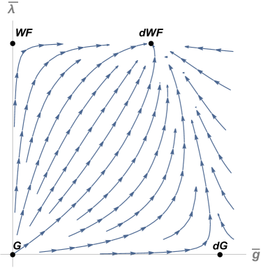
Figure 1: RG flow trajectories of (11) are shown for $N=\epsilon=1$. Here, $\bar{\lambda}=\lambda/\lambda_{\text{\tiny{WF}}}$ and $\bar{g}=g/g_{\text{\tiny{WF}}}$. Arrows indicate the direction towards the IR. The bold point at the origin (G) represents the infrared repulsive massless free vector model without defect. The Wilson-Fisher (WF) conformal field theory without defect and the Gaussian DCFT (dG) are denoted by solid dots on the $\bar{\lambda}$ and $\bar{g}$ axes, respectively. The solid dot denoted by dWF corresponds to the Wilson-Fisher fixed point with defect, ($g_{\text{\tiny{WF}}},\lambda_{\text{\tiny{WF}}}$), which serves as an IR attractor of the RG flows in the two-dimensional coupling space.

To determine the value of the anomaly constant $b$ for dWF, we examine the RG trajectory of (11) with $\lambda=\lambda_{\text{\tiny{WF}}}$. In this scenario, $\beta_{\lambda}=0$ throughout the flow, indicating that the bulk remains intact and is represented by the WF CFT. In contrast, the defect changes: it is trivial in the UV but is characterized by $g_{\text{\tiny{WF}}}\neq 0$ in the IR. This RG trajectory corresponds to a horizontal line connecting the WF fixed point on the $\lambda$-axis with dWF in Fig. 1. Therefore, for this specific RG trajectory, we can use the general result for the increment of $b$, as obtained in Shachar:2022fqk through conformal perturbation theory. In our context, it takes the form,

$$b_{\text{\tiny{WF}}}=-{N\over 8}\bar{\epsilon}^{3}+\mathcal{O}(\bar{\epsilon}^{4})~{},$$ (14)

where $\bar{\epsilon}=2-\Delta_{\phi^{2}}$, and $\Delta_{\phi^{2}}$ represents the scaling dimension of $\phi^{2}$ at the Wilson-Fisher fixed point, i.e.,

$$\bar{\epsilon}=-{{\partial}\beta_{g}\over{\partial}g}\bigg{|}_{g=0,~{}\lambda=\lambda_{\text{\tiny{WF}}}}={6\,\epsilon\over N+8}~{}.$$ (15)

In Appendix A, we perform a direct calculation of the partition function to independently verify the above value of $b_{\text{\tiny{WF}}}$. Similarly Shachar:2022fqk ,

$$b_{\text{\tiny{G}}}=-{N\over 8}\epsilon^{3}+\mathcal{O}(\epsilon^{4})~{}.$$ (16)

Hence, for all $N$, we obtain

$$b_{\text{\tiny{WF}}}-b_{\text{\tiny{G}}}=\frac{N\left(\epsilon^{3}-\bar{\epsilon}^{3}\right)}{8}>0~{},$$ (17)

leading to a violation of the naive generalization of the $b$-theorem under the RG flow from the dG to dWF.

4 Gross-Neveu-Yukawa model with a defect

Consider now the same two-dimensional spherical defect as in the previous section, but this time embedded in the $d=4-\epsilon$ dimensional bulk described by a single bosonic field, $\phi$, coupled to $N_{\text{F}}$ Dirac fields,

$$S=\int_{\mathcal{B}}~{}\Big{(}\bar{\psi}\not{\partial}\psi+\frac{1}{2}(\partial\phi)^{2}+\eta\,\mu^{\epsilon\over 2}\bar{\psi}\psi\phi+\frac{\lambda\mu^{\epsilon}}{4!}\phi^{4}\Big{)}+g\mu^{\epsilon}\int_{\mathcal{S}^{2}}\phi^{2}~{}.$$ (18)

This action describes the $U(N_{\text{\tiny F}})$ invariant Gross-Neveu-Yukawa (GNY) model with a two-dimensional spherical defect. To maintain brevity, we suppress the flavor index of the vector field $\psi$.

The RG flow in this model occurs in the three-dimensional space of couplings $(\eta,\lambda,g)$. The associated beta functions are derived in Appendix B, while here we present the final expressions

$$\beta_{\lambda} = -\epsilon\lambda+\frac{1}{8\pi^{2}}\Big{(}\,\frac{3}{2}\lambda^{2}+N\lambda\eta^{2}-6N\eta^{4}\Big{)}+\ldots~{},$$

$$\beta_{\eta^{2}} = -\epsilon\eta^{2}+\frac{N+6}{16\pi^{2}}\eta^{4}+\ldots~{},$$ (19)

$$\beta_{g} = -\epsilon g+\frac{g^{2}}{\pi}+\frac{g}{16\pi^{2}}\left(\lambda+N\eta^{2}\right)+\ldots~{},$$

where ellipses denote higher-order corrections in the small coupling constants. Here, $N=\text{Tr}(\mathbb{I}_{4\times 4})N_{\text{\tiny F}}=4N_{\text{\tiny F}}$ represents the total number of fermionic degrees of freedom in four dimensions. Notably, the RG flow equations (19) cannot be recovered using (6) because conformal perturbation theory in Section 3 is restricted to quadratic order in the coupling constants, where the knowledge of OPE coefficients is enough to recover the structure of the beta functions. In contrast, for consistency, the beta functions (19) must necessarily include quartic corrections in $\eta$.

The two-dimensional plane $\eta=0$ encompasses all the fixed points previously discussed in section 3. In addition to these, there exist two new fixed points: $(\eta_{*},\lambda_{*},g_{*})=(\eta_{\text{\tiny{GNY}}},\lambda_{\text{\tiny{GNY}}},g_{\text{\tiny{GNY}}})$ and $(\eta_{\text{\tiny{GNY}}},\lambda_{\text{\tiny{GNY}}},0)$, with and without defect, respectively, where

$$\eta_{\text{\tiny{GNY}}} = 4\pi\sqrt{\frac{\epsilon}{N+6}}~{},$$

$$\lambda_{\text{\tiny{GNY}}} = \frac{384\pi^{2}N\epsilon}{\left(N+6\right)\left(N-6+\sqrt{N^{2}+132N+36}\right)}~{},$$ (20)

$$g_{\text{\tiny{GNY}}} = \pi\epsilon\bigg{(}1-\frac{6+5N+\sqrt{N^{2}+132N+36}}{6\left(N+6\right)}\,\bigg{)}~{}.$$

The fixed point $(\eta_{\text{\tiny{GNY}}},\lambda_{\text{\tiny{GNY}}},0)$ belongs to the $g=0$ plane accommodating all possible RG flows without a defect. As shown in Fig. 2, this fixed point is an IR stable attractor of the RG trajectories restricted to this plane.

Analysis of the $3\times 3$ matrix of derivatives of the beta functions (19) leads to the conclusion that the previously IR attractive fixed point $(0,\lambda_{\text{\tiny{WF}}},g_{\text{\tiny{WF}}})$ becomes unstable under Yukawa deformation. Similarly, the critical GNY model without a defect becomes IR repulsive when introducing the $\phi^{2}$ deformation onto the two-dimensional defect surface. Furthermore, as depicted in Fig. 3, the DCFT characterized by $(\eta_{\text{\tiny{GNY}}},\lambda_{\text{\tiny{GNY}}},g_{\text{\tiny{GNY}}})$, denoted by dGNY in the figure, stands as the only IR stable fixed point in the three-dimensional coupling space of the GNY model with the type of defect studied in this section.

Figure 2: The plot depicts the $g=0$ plane accommodating RG flow trajectories without a defect, obtained from (20) for $N=\epsilon=1$. Here, $\bar{\lambda}=\lambda/\lambda_{\text{\tiny{GNY}}}$ and $\bar{\eta}=\eta/\eta_{\text{\tiny{GNY}}}$. Arrows indicate the direction towards the IR. The bold point at the origin represents the infrared repulsive Gaussian CFT (G) with a massless free scalar and $N_{\text{\tiny F}}$ massless Dirac fields. The solid dots on the $\bar{\lambda}$ axis and in the upper right corner denote the critical Wilson-Fisher (WF) and Gross-Neveu-Yukawa (GNY) models, respectively.

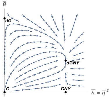
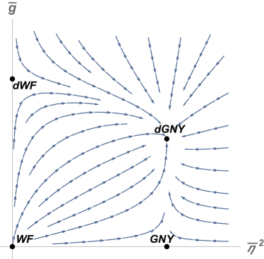
Figure 3: The plots display planar sections of RG flow trajectories obtained from (20) for $N=\epsilon=1$. Here, $\bar{\lambda}=\lambda/\lambda_{\text{\tiny{GNY}}}$, $\bar{\eta}=\eta/\eta_{\text{\tiny{GNY}}}$, and $\bar{g}=g/g_{\text{\tiny{GNY}}}$. Arrows indicate the direction towards the IR. The solid dot denoted by dGNY corresponds to the critical Gross-Neveu-Yukawa (GNY) model with a defect, $(\eta_{\text{\tiny{GNY}}},\lambda_{\text{\tiny{GNY}}},g_{\text{\tiny{GNY}}})$, serving as an IR attractor of the RG flows in the three-dimensional coupling space. The critical GNY model without a defect is represented by a solid dot on the horizontal axis. Left panel: Lines of RG flow are displayed in the $\bar{\lambda}=\bar{\eta}^{2}$ plane. The origin represents the infrared repulsive Gaussian CFT (G) with a massless free scalar and $N_{\text{\tiny F}}$ massless Dirac fields. The solid dot on the $\bar{g}$ axis denotes a Gaussian CFT with a non-trivial defect (dG). Right panel: Lines of RG flow are displayed in the $\bar{\lambda}=\bar{\eta}^{2}+\lambda_{\text{\tiny{WF}}}/\lambda_{\text{\tiny{GNY}}}(1-\bar{\eta}^{2})$ plane. The origin represents the infrared repulsive critical Wilson-Fisher (WF) fixed point without a defect. The solid dot on the $\bar{g}$ axis corresponds to WF with a non-trivial conformal defect (dWF).

The $b$-anomaly of the IR stable DCFT can be derived by considering the RG flow originating from $(\eta_{\text{\tiny{GNY}}},\lambda_{\text{\tiny{GNY}}},0)$ and terminating at $(\eta_{\text{\tiny{GNY}}},\lambda_{\text{\tiny{GNY}}},g_{\text{\tiny{GNY}}})$ with a fixed GNY bulk, $\eta=\eta_{\text{\tiny{GNY}}}$ and $\lambda=\lambda_{\text{\tiny{GNY}}}$, along the RG trajectory. This flow corresponds to a line parallel to the $\bar{g}$-axis in Fig. 3, connecting the critical GNY model without a defect with dGNY. Using the general result for the increment of $b$, as obtained in Shachar:2022fqk through conformal perturbation theory, yields

$$b_{\text{\tiny{GNY}}}=-{\bar{\epsilon}^{3}\over 8}+\mathcal{O}(\bar{\epsilon}^{4})~{},$$ (21)

where $\bar{\epsilon}=2-\Delta_{\phi^{2}}$, and $\Delta_{\phi^{2}}$ represents the scaling dimension of $\phi^{2}$ in the critical GNY model,

$$\bar{\epsilon}=-{{\partial}\beta_{g}\over{\partial}g}\bigg{|}_{(\eta_{\text{\tiny{GNY}}},\lambda_{\text{\tiny{GNY}}},0)}=\epsilon\bigg{(}1-\frac{6+5N+\sqrt{N^{2}+132N+36}}{6\left(N+6\right)}\,\bigg{)}~{}.$$ (22)

In Appendix A, we independently verify the above value for $b_{\text{\tiny{GNY}}}$ through a direct calculation of the partition function.

For $N=0$, the anomaly takes the value of $b_{\text{\tiny{GNY}}}|_{N=0}=-\frac{\epsilon^{3}}{27}$, which, as expected, matches $b\text{\tiny{WF}}$ in (14) for a single boson. It then increases with $N$ and vanishes at $N=12$. Consequently, for $N<12$ the naive generalization of the $b$-theorem is violated for two distinct RG flows that end at $(\eta_{\text{\tiny{GNY}}},\lambda_{\text{\tiny{GNY}}},g_{\text{\tiny{GNY}}})$. The first scenario where it is violated, occurs when the flow starts at dG, leading to an increase in the value of $b$ for all $N<12$, see left panel of Fig. 3. In the second scenario, the anomaly increases for any strictly positive $N<12$ when the flow starts at dWF and terminates at dGNY, see right panel of Fig. 3.

Moreover, as $g_{\text{\tiny{GNY}}}$ vanishes in the limit $N\to 12$, the fixed point dGNY in Fig. 3 merges with the critical GNY model without a defect. Consequently, the violation occurs when either dWF or dG are deformed by the Yukawa coupling in the bulk because both DCFTs with negative anomaly flow towards the critical GNY model without an anomaly. This scenario is depicted in Fig. 4.

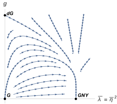
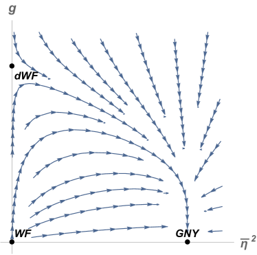
Figure 4: The plots depict planar sections of RG flow trajectories, obtained from (20) for $N=12$ and $\epsilon=1$. Here, $\bar{\lambda}=\lambda/\lambda_{\text{\tiny{GNY}}}$ and $\bar{\eta}=\eta/\eta_{\text{\tiny{GNY}}}$. Arrows indicate the direction towards the IR. The critical GNY model without a defect is represented by a solid dot on the horizontal axis. For $N=12$, this fixed point is an IR stable attractor of the RG flows in the three-dimensional coupling space. Left panel: Lines of RG flow are displayed in the $\bar{\lambda}=\bar{\eta}^{2}$ plane. The origin represents the infrared repulsive Gaussian CFT (G) with a massless free scalar and $N_{\text{\tiny F}}$ massless Dirac fields. The solid dot on the $g$ axis denotes a Gaussian CFT with a non-trivial defect (dG). Right panel: Lines of RG flow are displayed in the $\bar{\lambda}=\lambda_{\text{\tiny{WF}}}/\lambda_{\text{\tiny{GNY}}}=1$ plane. The origin represents the infrared repulsive critical Wilson-Fisher (WF) fixed point without a defect. The solid dot on the $g$ axis corresponds to WF with a non-trivial conformal defect (dWF).

Finally, when $N>12$, the coupling $g_{\text{\tiny{GNY}}}$ becomes negative and gradually approaches zero as $N$ tends to infinity. In this range, the $b$-anomaly of the dGNY model acquires small positive values. Neither dG nor dWF flows towards dGNY under these circumstances. However, the flow from the Gaussian fixed point (G) without a defect still terminates at the dGNY, thereby violating the naive generalization of the $b$-theorem. This case warrants caution, as a negative $g_{\text{\tiny{GNY}}}$ implies the possibility of nontrivial classical profiles in the bulk Giombi2023 ; RavivMoshe2023 , accompanied by symmetry breaking. While studying this phenomenon is interesting, we have chosen to leave it outside the scope of the current work.

5 Discussion

In this paper, we discussed a violation of the naive generalisation of the $b$-theorem, to the case of simultaneous bulk and defect RG flows, in a quantum system defined on a $d$-dimensional flat bulk coupled to a $2d$ defect. We demonstrated said violation in two distinct models namely, the $O(N)$ vector model and the Gross-Neveu-Yukawa (GNY) model, each coupled to a two-dimensional spherical defect. The computation of the $b$-anomaly at the various fixed points in each of these models was done using conformal perturbation theory, and the result was verified from an independent computation of the free energy in each system.

The failure to generalise the $b$-theorem to the case of simultaneous bulk-defect RG flows is reminiscent of a similar violation of the $g$-theorem Green:2007wr , which characterises RG flows on $1d$ boundaries of $2d$ critical systems. In case of $1d$ boundaries/defects, the $g$-function is interpreted as the impurity entropy, that can either increase or decrease under bulk interactions. Such an interpretation provides a clear physical understanding underlying the failure to generalise the $g$-theorem to include bulk RG flows. Finding a similar understanding in the context of the $b$-theorem remains one of the interesting open problems.

Another challenging open question that follows from such a violation, is regarding the existence and construction of an altogether different class of $C$- functions for defect QFTs, that follow from the partition function, and that again display monotonicity properties under simultaneous bulk and defect RG flows.

A completely independent, alternate construction of the $C$-functions for boundaries and defects was provided using information theoretic techniques (such as relative entropy, entanglement entropy and the Quantum Null Energy Condition) in Casini:2023kyj . It will be interesting to explore whether such measures can capture the violation of the $g$-theorem and the $b$-theorem under simultaneous bulk-defect RG flows.

Acknowledgements We thank Chris Herzog and Maxime Trépanier for helpful discussions and correspondence. TS and MS acknowledge partial support from the Israel Science Foundation (ISF) Center for Excellence grant (Grant Number 2289/18), BSF Grant No. 2022113, and NSF-BSF Grant No. 2022726. Additionally, MS acknowledges partial support from Israel’s Council for Higher Education. RS is supported by the Royal Society-Newton International Fellowship NIF/R1/221054-Royal Society.

Appendix A Computation of the $b$-anomaly

Another method of calculating the $b$-anomaly is based on evaluating the free energy. For a two-dimensional spherical conformal defect embedded in flat space, the free energy is given by,

$$\mathcal{F}=\mathcal{F}_{\text{\tiny CFT}}-\frac{b}{3}\log\left(\mu R\right)+\ldots~{}.$$ (23)

Here, $\mathcal{F}_{\text{\tiny CFT}}$ represents the free energy of the ambient CFT without the defect, $R$ corresponds to the radius of the sphere, and the ellipsis denotes non-universal terms that depend on the specific scheme used.

In this appendix, we perform a direct evaluation of the free energy for the $O(N)$ vector model (7) and the GNY model (18), from which we extract the values of $b\text{\tiny{WF}}$ and $b_{\text{\tiny{GNY}}}$, respectively. The final results agree with (14) and (21), derived based on perturbative calculations of the defect stress tensor two-point function Shachar:2022fqk .

Starting from the Gaussian $O(N)$ vector model (7) without defects, we introduce an $O(N)$-invariant quartic interaction throughout the bulk and a $\phi^{2}$ term supported solely on the two-dimensional sphere of radius $R$. This deformation drives the system towards the $(g_{\text{\tiny{WF}}},\lambda_{\text{\tiny{WF}}})$ fixed-point in the deep infrared (IR). As illustrated in Fig.1, this fixed-point is the only admissible IR endpoint of the RG flow when both deformations are present. Due to the weak coupling of the fixed point, we can expand the free energy in the IR as follows

$$\mathcal{F} =-\log\left[\int\,[\mathcal{D}\phi]~{}e^{-S_{CFT}-g_{0}\int_{\mathcal{S}^{2}}\phi^{2}-\lambda_{0}\int_{\mathcal{B}}~{}(\phi^{2})^{2}}\right]$$

$$=\mathcal{F}_{\lambda_{0}}-\log\left(1-g_{0}\int_{\mathcal{S}^{2}}\langle\phi^{2}\rangle_{\lambda_{0}}+\frac{g_{0}^{2}}{2}\int_{\mathcal{S}^{2}}\int_{\mathcal{S}^{2}}\langle\phi^{2}(\sigma_{1})\phi^{2}(\sigma_{2})\rangle_{\lambda_{0}}\right.$$

$$\left.-\frac{g_{0}^{3}}{3!}\int_{\mathcal{S}^{2}}\int_{\mathcal{S}^{2}}\int_{\mathcal{S}^{2}}\langle\phi^{2}(\sigma_{1})\phi^{2}(\sigma_{2})\phi^{2}(\sigma_{3})\rangle_{\lambda_{0}}+\dots\right)$$

$$=\mathcal{F}_{\lambda_{0}}-\frac{g_{0}^{2}}{2}\int_{\mathcal{S}^{2}}\int_{\mathcal{S}^{2}}\langle\phi^{2}(\sigma_{1})\phi^{2}(\sigma_{2})\rangle_{0}+\frac{g_{0}^{2}\lambda_{0}}{2}\int_{\mathcal{S}^{2}}\int_{\mathcal{S}^{2}}\int_{\mathcal{B}}~{}\langle\phi^{2}(\sigma_{1})\phi^{2}(\sigma_{2})(\phi^{2})^{2}(x_{3})\rangle_{0}$$

$$+\frac{g_{0}^{3}}{3!}\int_{\mathcal{S}^{2}}\int_{\mathcal{S}^{2}}\int_{\mathcal{S}^{2}}\langle\phi^{2}(\sigma_{1})\phi^{2}(\sigma_{2})\phi^{2}(\sigma_{3})\rangle_{0}+\ldots~{},$$ (24)

where $\mathcal{F}_{\lambda_{0}}=\mathcal{F}|_{g_{0}=0}$ is anomaly-free, and in the last equality of (A), we dropped $\langle\phi^{2}\rangle_{\lambda_{0}}$ because this term is power-law divergent, and therefore it vanishes in dimensional regularization. Thus,

$$\Delta\mathcal{F}\equiv\mathcal{F}-\mathcal{F}_{\lambda_{0}}=-\frac{g_{0}^{2}}{2}J_{1}+\frac{g_{0}^{2}\lambda_{0}}{2}J_{2}+\frac{g_{0}^{3}}{3!}J_{3}+\ldots~{}.$$ (25)

Here,

$$J_{1} = \int_{\mathcal{S}^{2}}\int_{\mathcal{S}^{2}}\langle\phi^{2}(\sigma_{1})\phi^{2}(\sigma_{2})\rangle_{0}~{},$$

$$J_{2} = \int_{\mathcal{S}^{2}}\int_{\mathcal{S}^{2}}\int_{\mathcal{B}}\langle\phi^{2}(\sigma_{1})\phi^{2}(\sigma_{2})\phi^{3}(x_{3})\rangle_{0}~{},$$ (26)

$$J_{3} = \int_{\mathcal{S}^{2}}\int_{\mathcal{S}^{2}}\int_{\mathcal{S}^{2}}\langle\phi^{2}(\sigma_{1})\phi^{2}(\sigma_{2})\phi^{3}(\sigma_{3})\rangle_{0}~{}.$$

Before proceeding with the computation of these expressions, let us review some useful identities. Denoting the length of the cord connecting two points $\sigma_{1},\sigma_{2}$ on $\mathcal{S}^{2}$ embedded in $\mathbb{R}^{d}$ as $s\left(\sigma_{1},\sigma_{2}\right)$, the following integrals hold Cardy:1988cwa ; Shachar:2022fqk ; Klebanov2011 ,

$$I_{1}\left(\alpha\right)=\int_{\mathcal{S}^{2}}\int_{\mathcal{S}^{2}}\frac{1}{s\left(\sigma_{1},\sigma_{2}\right)^{2\alpha}}=\frac{\pi^{2}\left(2R\right)^{4-2\alpha}}{1-\alpha}~{},$$ (27)

$$I_{2}\left(\alpha\right)=\int_{\mathcal{S}^{2}}\int_{\mathcal{S}^{2}}\int_{\mathcal{S}^{2}}\frac{1}{\left[s(\sigma_{1},\sigma_{2})s(\sigma_{2},\sigma_{3})s(\sigma_{3},\sigma_{1})\right]^{\alpha}}=\frac{8\pi^{9/2}\Gamma\left(2-\frac{3\alpha}{2}\right)R^{6-3\alpha}}{\Gamma\left(\frac{3-\alpha}{2}\right)^{3}}~{}.$$ (28)

In addition, we are going to use the conformal merging relation Goykhman2021 ,

$$\int d^{d}x_{2}\frac{1}{\left|x_{12}\right|^{2\Delta_{1}}\left|x_{23}\right|^{2\Delta_{2}}}=\frac{U\left(\Delta_{1},\Delta_{2},d-\Delta_{1}-\Delta_{2}\right)}{\left|x_{13}\right|^{2\Delta_{1}+2\Delta_{2}-d}}~{},$$ (29)

where $x_{12}=x_{1}-x_{2}$ and

$$U\left(\Delta_{1},\Delta_{2},\Delta_{3}\right)=\pi^{\frac{d}{2}}\frac{\Gamma\left(\frac{d}{2}-\Delta_{1}\right)\Gamma\left(\frac{d}{2}-\Delta_{2}\right)\Gamma\left(\frac{d}{2}-\Delta_{3}\right)}{\Gamma\left(\Delta_{1}\right)\Gamma\left(\Delta_{2}\right)\Gamma\left(\Delta_{3}\right)}~{}.$$ (30)

Using the above identities, we obtain

$$J_{1} = 2NC_{\phi}^{2}~{}I_{1}\left(2-\epsilon\right)=-(2R)^{2\epsilon}\frac{N}{8\pi^{2}}+\ldots~{},$$

$$J_{2} = 8N(N+2)C_{\phi}^{4}\,U\left(2-\epsilon,2-\epsilon,\epsilon\right)I_{1}\Big{(}2-\frac{3}{2}\epsilon\Big{)}=-(2R)^{3\epsilon}\frac{N(N+2)}{8\pi^{4}\epsilon}+\ldots~{},$$

$$J_{3} = 8NC_{\phi}^{3}~{}I_{2}(2-\epsilon)=-R^{3\epsilon}\left(\frac{2N}{3\pi^{3}\epsilon}\right)+\ldots~{}.$$ (31)

Combining everything and using (5) and (10) to express the bare parameters in (25) in terms of the renormalized ones yields,

$$\Delta\mathcal{F}= \frac{N}{8\pi^{2}}\frac{g^{2}}{2}\left(2\mu R\right)^{2\epsilon}\left(1+\frac{g}{\pi\epsilon}+\frac{\lambda(N+2)}{2\pi^{2}\epsilon}\right)^{2}$$

$$-(2\mu R)^{3\epsilon}\frac{g^{2}\lambda}{2}\frac{N(N+2)}{8\pi^{4}\epsilon}-(\mu R)^{3\epsilon}\frac{g^{3}}{6}\left(\frac{2N}{3\pi^{3}\epsilon}\right)+\ldots~{}.$$ (32)

Identifying the coefficient of $\log(\mu R)$ and plugging in the critical values (13) yields,

$$b_{\text{\tiny{WF}}} =\left(-\frac{3N\epsilon}{8\pi^{2}}g^{2}+\frac{N}{4\pi^{3}}g^{3}+\frac{3N(N+2)}{16\pi^{4}}g^{2}\lambda\right)\bigg{|}_{\lambda_{*}=\lambda_{\text{\tiny{WF}}},~{}g_{*}=g_{\text{\tiny{WF}}}}$$

$$=-\frac{27N}{(N+8)^{3}}\epsilon^{3}+\ldots~{}.$$ (33)

In agreement with (14).

To conclude this appendix, we compute the free energy for the GNY model. The computation follows in the same way as before, with an additional integral that requires evaluation,

$$\Delta\mathcal{F}=-\frac{g_{0}^{2}}{2}J_{1}+\frac{g_{0}^{2}\lambda_{0}}{2\cdot 4!}J_{2}+\frac{g_{0}^{3}}{3!}J_{3}-\frac{g_{0}^{2}\eta_{0}^{2}}{4}J_{4}+\ldots~{}.$$ (34)

This integral is given by

$$J_{4}= \int_{\mathcal{S}^{2}}\int_{\mathcal{S}^{2}}\int_{\mathcal{B}}\int_{\mathcal{B}}~{}\langle\phi_{0}^{2}\left(\sigma_{1}\right)\phi_{0}^{2}\left(\sigma_{2}\right)\bar{\psi}_{0}\psi_{0}\phi_{0}\left(x_{1}\right)\bar{\psi}_{0}\psi_{0}\phi_{0}\left(x_{2}\right)\rangle_{0}$$

$$=8N\,C^{3}_{\phi}C^{2}_{\psi}~{}U\left(\frac{2-\epsilon}{2},3-\epsilon,\frac{\epsilon}{2}\right)U\left(\frac{2-\epsilon}{2},2-\epsilon,1+\frac{\epsilon}{2}\right)I_{1}\left(2-\frac{3\epsilon}{2}\right)$$

$$=(2R)^{3\epsilon}\frac{N}{32\pi^{4}\epsilon}+\ldots~{},$$ (35)

where we employed the conformal merging relation (29) twice, and used the position space representation of the two-point function for a massless Dirac field,

$$\langle\psi(x_{1})\bar{\psi}(x_{2})\rangle=C_{\psi}{\not{x}_{12}\over|x_{12}|^{d}}~{},\quad C_{\psi}={\Gamma\left({d\over 2}\right)\over 2\pi^{d\over 2}}~{}.$$ (36)

In addition, the Yukawa interaction contributes to the first term of (34) through the following renormalization of the coupling (see Appendix B)

$$g_{0}=g\mu^{\epsilon}\left(1+\frac{g}{\pi\epsilon}+\frac{\lambda}{16\pi^{2}\epsilon}+\frac{N\eta^{2}}{16\pi^{2}\epsilon}+\ldots\right)~{}.$$ (37)

Overall, we find,

$$b_{\text{\tiny{GNY}}} =\left(-\frac{3\epsilon}{8\pi^{2}}g^{2}+\frac{1}{4\pi^{3}}g^{3}+\frac{3}{128\pi^{4}}g^{2}\lambda+\frac{3Ng^{2}\eta^{2}}{128\pi^{4}}\right)\bigg{|}_{\eta_{*}=\eta_{\text{\tiny{GNY}}},~{}\lambda_{*}=\lambda_{\text{\tiny{GNY}}},~{}g_{*}=g_{\text{\tiny{GNY}}}}+\ldots$$

$$=-{\epsilon^{3}\over 8}\bigg{(}1-\frac{6+5N+\sqrt{N^{2}+132N+36}}{6\left(N+6\right)}\,\bigg{)}^{3}+\ldots~{}.$$ (38)

This expression agrees with (21).

Appendix B RG beta functions for GNY model with defect

To renormalize the GNY model, we supplement its action (18) with the following counterterms

$$S_{\text{c.t.}}=\int_{\mathcal{B}}~{}\Big{(}\delta Z_{\psi}\bar{\psi}\not{\partial}\psi+\frac{\delta Z_{\phi}}{2}(\partial\phi)^{2}+\delta Z_{\eta}\,\eta\,\mu^{\frac{\epsilon}{2}}\,\bar{\psi}\psi\phi+\frac{\delta Z_{\lambda}}{4!}\,\lambda\,\mu^{\epsilon}\phi^{4}\Big{)}+\delta Z_{g}\,g\,\mu^{\epsilon}\int_{\mathcal{S}^{2}}\phi^{2}~{},$$ (39)

where all couplings are dimensionless and $\delta Z_{i}$ for $i=\psi,\phi,\eta,\lambda,g$ contain an ascending series of poles in $1/\epsilon$; that is, we employ the minimal subtraction scheme. Define $Z_{i}=1+\delta Z_{i}$, then the relations between the bare and renormalized parameters are given by

$$\psi_{0}=\sqrt{Z_{\psi}}\,\psi,\qquad\phi_{0}=\sqrt{Z_{\phi}}\,\phi~{},$$ (40)

$$\eta_{0}={Z_{\eta}\over\sqrt{Z_{\phi}}Z_{\psi}}\,\mu^{\frac{\epsilon}{2}}\,\eta,\qquad\lambda_{0}={Z_{\lambda}\over Z^{2}_{\phi}}~{}\mu^{\epsilon}\lambda,\qquad g_{0}={Z_{g}\over Z_{\phi}}~{}\mu^{\epsilon}g~{}.$$ (41)

In this appendix, we carry out explicit calculations of the 1-loop Feynman graphs contributing to renormalization constants $Z_{i}$.

Figure 5: One-loop diagrams contributing to the wave function renormalization in the GNY model for (a) the scalar field $\phi$ and (b) the Dirac field $\psi$. Internal solid lines with arrows correspond to the propagator of the Dirac field, while internal dashed lines represent the propagator of the scalar field. External dashed and solid lines denote scalar and Dirac background fields, respectively.

The wave function renormalization of the scalar and Dirac fields are associated with the diagrams in Fig.5,

Fig.5(a) $$= -{N_{\text{\tiny F}}\eta^{2}\mu^{\epsilon}\,C_{\psi}^{2}\over 2}\int_{\mathcal{B}}\int_{\mathcal{B}}\phi(x_{1})\phi(x_{2})\text{tr}\Big{(}{\not{x}_{12}\not{x}_{21}\over|x_{12}|^{d}|x_{21}|^{d}}\Big{)}=-{N\eta^{2}\over 32\pi^{2}\epsilon}\int_{\mathcal{B}}{\partial}\phi{\partial}\phi+\ldots~{},$$

Fig.5(b) $$= \eta^{2}\mu^{\epsilon}C_{\psi}C_{\phi}\int_{\mathcal{B}}\int_{\mathcal{B}}{\bar{\psi}(x_{1})\not{x}_{12}\psi(x_{2})\over(x_{12}^{2})^{d-1}}=-{\eta^{2}\over 16\pi^{2}\epsilon}\int_{\mathcal{B}}\bar{\psi}\not{\partial}\psi+\ldots~{}.$$

where $x_{12}=x_{1}-x_{2}$, $N=4N_{\text{F}}$ is the total number of fermionic degrees of freedom in four dimensions, the trace is done over the spinor indices, and we used (36). Hence,

$$Z_{\phi}=1-\frac{N\eta^{2}}{16\pi^{2}\epsilon}+\ldots~{},$$

$$Z_{\psi}=1-{\eta^{2}\over 16\pi^{2}\epsilon}+\ldots~{}.$$ (42)

Figure 6: One-loop diagram contributing to the renormalization of the Yukawa coupling $\eta$ in the GNY model. Internal solid lines with arrows correspond to the propagator of the Dirac field $\psi$, while the internal dashed line represents the propagator of the scalar field $\phi$. In contrast, external dashed and solid lines denote scalar and Dirac background fields, respectively.

Next, we fix $Z_{\eta}$ by evaluating the one-loop diagram in Fig. 6,

$$\text{Fig.}\ref{fig:Zeta}=-\eta^{3}\mu^{3\epsilon\over 2}C_{\psi}^{2}C_{\phi}\int_{\mathcal{B}}\int_{\mathcal{B}}\int_{\mathcal{B}}\phi(x_{1}){\bar{\psi}(x_{2})\not{x}_{21}\not{x}_{13}\psi(x_{3})\over|x_{21}|^{d}|x_{31}|^{d}|x_{23}|^{d-2}}~{}.$$ (43)

The pole in $\epsilon$ of this integral is obtained by expanding the Dirac fields around $x_{1}$ and subsequently integrating over $x_{2}$ and $x_{3}$ using the scalar-fermion propagator merging relation of the form

$$\int d^{d}x_{3}{\not{x}_{31}\over|x_{31}|^{2\Delta_{1}+1}|x_{23}|^{2\Delta_{2}}} = {\pi^{d\over 2}\Gamma\left({d\over 2}-\Delta_{2}\right)\Gamma\left({d\over 2}-\Delta_{1}+{1\over 2}\right)\Gamma\left(\Delta_{1}+\Delta_{2}-{d\over 2}+{1\over 2}\right)\over\Gamma(\Delta_{2})\Gamma\left(\Delta_{1}+{1\over 2}\right)\Gamma\left(d-\Delta_{1}-\Delta_{2}+{1\over 2}\right)}$$ (44)

$$\times {\not{x}_{21}\over|x_{12}|^{2(\Delta_{1}+\Delta_{2})-d+1}}~{}.$$

The final expression is given by

$$\text{Fig.}\ref{fig:Zeta}={\eta^{3}\mu^{\epsilon\over 2}\over 8\pi^{2}\epsilon}\int_{\mathcal{B}}\bar{\psi}\psi\phi+\ldots~{}.$$ (45)

Thus

$$Z_{\eta}=1+{\eta^{2}\over 8\pi^{2}\epsilon}+\ldots~{}.$$ (46)

Substituting (42) and (46) into the relation between $\eta_{0}$ and $\eta$ in (41), gives ZinnJustin1991 ; Moshe2003

$$\eta_{0}={Z_{\eta}\over\sqrt{Z_{\phi}}Z_{\psi}}\,\mu^{\frac{\epsilon}{2}}\,\eta\quad\Rightarrow\quad\beta_{\eta^{2}}=-\epsilon\eta^{2}+\frac{N+6}{16\pi^{2}}\eta^{4}~{}.$$ (47)

To derive the RG flow for $\lambda$, one has to consider the one-loop diagrams shown in Fig. 7

Fig.7(a) $$= {\lambda^{2}\mu^{2\epsilon}C_{\phi}^{2}\over 16}\int_{\mathcal{B}}\int_{\mathcal{B}}{\phi^{2}(x_{1})\phi^{2}(x_{2})\over|x_{12}|^{2(d-2)}}~{},$$ (48)

Fig.7(b) $$= -{\eta^{4}\mu^{2\epsilon}C_{\psi}^{4}N_{\text{\tiny F}}\over 4}\int_{\mathcal{B}}\int_{\mathcal{B}}\int_{\mathcal{B}}\int_{\mathcal{B}}\prod_{i=1}^{4}\phi(x_{i})\text{tr}\left({\not{x}_{12}\not{x}_{23}\not{x}_{34}\not{x}_{41}\over|x_{12}|^{d}|x_{23}|^{d}|x_{34}|^{d}|x_{41}|^{d}}\right)~{}.$$

Figure 7: Two one-loop diagrams contributing to the renormalization of the coupling $\lambda$ in the GNY model. Internal solid lines with arrows correspond to the propagator of the Dirac field $\psi$, while the internal dashed lines represent the propagator of the scalar field $\phi$. External dashed and solid lines denote scalar and Dirac background fields, respectively.

The counterterm $Z_{\lambda}$ is entirely fixed by the poles in $\epsilon$, therefore we expand the background fields around $x_{1}$ and get

Fig.7(a) $$= {\lambda^{2}\mu^{\epsilon}\over 128\pi^{2}\epsilon}\int_{\mathcal{B}}\phi^{4}+\ldots~{},$$

Fig.7(b) $$= -{\eta^{4}\mu^{\epsilon}N\over 32\pi^{2}\epsilon}\int_{\mathcal{B}}\phi^{4}+\ldots~{}.$$ (49)

To get the above expression for Fig. 7(b), we used (44) and the merging relation for the pair of Dirac propagators,

$$\int d^{d}x_{3}{\not{x}_{13}\not{x}_{32}\over|x_{32}|^{2\Delta_{1}+1}|x_{13}|^{2\Delta_{2}+1}} = {-\pi^{d\over 2}\Gamma\left(\Delta_{1}+\Delta_{2}-{d\over 2}\right)\Gamma\left({d\over 2}-\Delta_{1}+{1\over 2}\right)\Gamma\left({d\over 2}-\Delta_{2}+{1\over 2}\right)\over\Gamma(d-\Delta_{1}-\Delta_{2})\Gamma\left(\Delta_{1}+{1\over 2}\right)\Gamma\left(\Delta_{2}+{1\over 2}\right)}$$ (50)

$$\times {\mathbb{I}_{[{d\over 2}]\times[{d\over 2}]}\over|x_{12}|^{2(\Delta_{1}+\Delta_{2})-d}}~{},$$

where $\mathbb{I}$ is an identity matrix in the spinor space. Hence,

$$Z_{\lambda}=1+{3\lambda\over 16\pi^{2}\epsilon}-{3\eta^{4}N\over 4\pi^{2}\lambda\,\epsilon}+\ldots~{}.$$ (51)

As a result, we obtain the following RG flow for $\lambda$ ZinnJustin1991 ; Moshe2003 ,

$$\lambda_{0}={Z_{\lambda}\over Z^{2}_{\phi}}~{}\mu^{\epsilon}\lambda\quad\Rightarrow\quad\beta_{\lambda}=-\epsilon\lambda+\frac{1}{8\pi^{2}}\Big{(}\frac{3}{2}\lambda^{2}+N\lambda\eta^{2}-6N\eta^{4}\Big{)}~{}.$$ (52)

Figure 8: Two one-loop diagrams contributing to the renormalization of the defect coupling $g$ in the GNY model. The double line represents the two-dimensional defect, while the internal and external dashed lines represent the propagator of the scalar field $\phi$ and external scalar background, respectively.

Finally, the leading non-trivial corrections to $Z_{g}$ come from the two diagrams shown in Fig. 8,

Fig.8(a) $$= 2\,C_{\phi}\,\mu^{2\epsilon}g^{2}\int_{\mathcal{S}^{2}}\int_{\mathcal{S}^{2}}{\phi(x_{1})\phi(x_{2})\over|x_{1}-x_{2}|^{2-\epsilon}}={\mu^{\epsilon}g^{2}\over\pi\epsilon}\int_{\mathcal{S}^{2}}\phi^{2}(x_{1})+\ldots$$ (53)

Fig.8(b) $$= {C_{\phi}^{2}\,\mu^{2\epsilon}\lambda g\over 2}\int_{\mathcal{S}^{2}}\int d^{d}x_{2}\,{\phi^{2}(x_{2})\over|x_{1}-x_{2}|^{4-2\epsilon}}={\mu^{\epsilon}g\lambda\over 16\pi^{2}\epsilon}\int_{\mathcal{S}^{2}}\phi^{2}(x_{1})+\ldots~{}.$$

Hence,

$$Z_{g}=1+\frac{g}{\pi\epsilon}+\frac{\lambda}{16\pi^{2}\epsilon}+\ldots~{}.$$ (54)

Substituting $Z_{g}$ and $Z_{\phi}$ from (42) into the relation between the bare $g_{0}$ and renormalized $g$ in (41) yields

$$g_{0}={Z_{g}\over Z_{\phi}}~{}\mu^{\epsilon}g\quad\Rightarrow\quad\beta_{g}=-\epsilon g+\frac{g^{2}}{\pi}+\frac{g}{16\pi^{2}}\left(\lambda+N\eta^{2}\right)~{}.$$ (55)

This beta function is new; it was not considered before in the literature.

References

- (1) A. B. Zamolodchikov, “Irreversibility of the Flux of the Renormalization Group in a 2D Field Theory,” JETP Lett. 43 (1986) 730–732.
- (2) J. L. Cardy, “Is There a c Theorem in Four-Dimensions?,” Phys. Lett. B 215 (1988) 749–752.
- (3) A. Cappelli, D. Friedan, and J. I. Latorre, “C theorem and spectral representation,” Nucl. Phys. B 352 (1991) 616–670.
- (4) H. Osborn, “Weyl consistency conditions and a local renormalization group equation for general renormalizable field theories,” Nucl. Phys. B 363 (1991) 486–526.
- (5) R. C. Myers and A. Sinha, “Holographic c-theorems in arbitrary dimensions,” JHEP 01 (2011) 125, arXiv:1011.5819 [hep-th].
- (6) D. L. Jafferis, I. R. Klebanov, S. S. Pufu, and B. R. Safdi, “Towards the F-Theorem: N=2 Field Theories on the Three-Sphere,” JHEP 06 (2011) 102, arXiv:1103.1181 [hep-th].
- (7) Z. Komargodski and A. Schwimmer, “On Renormalization Group Flows in Four Dimensions,” JHEP 12 (2011) 099, arXiv:1107.3987 [hep-th].
- (8) Z. Komargodski, “The Constraints of Conformal Symmetry on RG Flows,” JHEP 07 (2012) 069, arXiv:1112.4538 [hep-th].
- (9) H. Casini and M. Huerta, “On the RG running of the entanglement entropy of a circle,” Phys. Rev. D 85 (2012) 125016, arXiv:1202.5650 [hep-th].
- (10) H. Elvang, D. Z. Freedman, L.-Y. Hung, M. Kiermaier, R. C. Myers, and S. Theisen, “On renormalization group flows and the a-theorem in 6d,” JHEP 10 (2012) 011, arXiv:1205.3994 [hep-th].
- (11) K. Yonekura, “Perturbative c-theorem in d-dimensions,” JHEP 04 (2013) 011, arXiv:1212.3028 [hep-th].
- (12) B. Grinstein, A. Stergiou, and D. Stone, “Consequences of Weyl Consistency Conditions,” JHEP 11 (2013) 195, arXiv:1308.1096 [hep-th].
- (13) I. Jack and H. Osborn, “Constraints on RG Flow for Four Dimensional Quantum Field Theories,” Nucl. Phys. B 883 (2014) 425–500, arXiv:1312.0428 [hep-th].
- (14) S. Giombi and I. R. Klebanov, “Interpolating between and ,” JHEP 03 (2015) 117, arXiv:1409.1937 [hep-th].
- (15) I. Jack, D. R. T. Jones, and C. Poole, “Gradient flows in three dimensions,” JHEP 09 (2015) 061, arXiv:1505.05400 [hep-th].
- (16) C. Cordova, T. T. Dumitrescu, and K. Intriligator, “Anomalies, renormalization group flows, and the a-theorem in six-dimensional (1, 0) theories,” JHEP 10 (2016) 080, arXiv:1506.03807 [hep-th].
- (17) H. Casini, M. Huerta, R. C. Myers, and A. Yale, “Mutual information and the F-theorem,” JHEP 10 (2015) 003, arXiv:1506.06195 [hep-th].
- (18) H. Casini, E. Testé, and G. Torroba, “Markov Property of the Conformal Field Theory Vacuum and the a Theorem,” Phys. Rev. Lett. 118 no. 26, (2017) 261602, arXiv:1704.01870 [hep-th].
- (19) M. Fluder and C. F. Uhlemann, “Evidence for a 5d F-theorem,” JHEP 02 (2021) 192, arXiv:2011.00006 [hep-th].
- (20) L. V. Delacretaz, A. L. Fitzpatrick, E. Katz, and M. T. Walters, “Thermalization and hydrodynamics of two-dimensional quantum field theories,” SciPost Phys. 12 no. 4, (2022) 119, arXiv:2105.02229 [hep-th].
- (21) J. L. Cardy, “Conformal Invariance and Surface Critical Behavior,” Nucl. Phys. B 240 (1984) 514–532.
- (22) J. L. Cardy, “Boundary Conditions, Fusion Rules and the Verlinde Formula,” Nucl. Phys. B 324 (1989) 581–596.
- (23) D. M. McAvity and H. Osborn, “Conformal field theories near a boundary in general dimensions,” Nucl. Phys. B 455 (1995) 522–576, arXiv:cond-mat/9505127.
- (24) I. Affleck, “Conformal field theory approach to the Kondo effect,” Acta Phys. Polon. B 26 (1995) 1869–1932, arXiv:cond-mat/9512099.
- (25) S. Sachdev, C. Buragohain, and M. Vojta, “Quantum impurity in a nearly critical two dimensional antiferromagnet,”. https://arxiv.org/abs/cond-mat/0004156.
- (26) M. Vojta, C. Buragohain, and S. Sachdev, “Quantum impurity dynamics in two-dimensional antiferromagnets and superconductors,” Physical Review B 61 no. 22, (Jun, 2000) 15152–15184. https://doi.org/10.1103%2Fphysrevb.61.15152.
- (27) J. Polchinski and J. Sully, “Wilson Loop Renormalization Group Flows,” JHEP 10 (2011) 059, arXiv:1104.5077 [hep-th].
- (28) D. Gaiotto, D. Mazac, and M. F. Paulos, “Bootstrapping the 3d Ising twist defect,” JHEP 03 (2014) 100, arXiv:1310.5078 [hep-th].
- (29) M. Billò, V. Goncalves, E. Lauria, and M. Meineri, “Defects in conformal field theory,” JHEP 04 (2016) 091, arXiv:1601.02883 [hep-th].
- (30) L. Bianchi, M. Meineri, R. C. Myers, and M. Smolkin, “Rényi entropy and conformal defects,” JHEP 07 (2016) 076, arXiv:1511.06713 [hep-th].
- (31) S. N. Solodukhin, “Boundary terms of conformal anomaly,” Phys. Lett. B 752 (2016) 131–134, arXiv:1510.04566 [hep-th].
- (32) D. V. Fursaev and S. N. Solodukhin, “Anomalies, entropy and boundaries,” Phys. Rev. D 93 no. 8, (2016) 084021, arXiv:1601.06418 [hep-th].
- (33) E. Lauria, M. Meineri, and E. Trevisani, “Spinning operators and defects in conformal field theory,” JHEP 08 (2019) 066, arXiv:1807.02522 [hep-th].
- (34) A. Gadde, “Conformal constraints on defects,” JHEP 01 (2020) 038, arXiv:1602.06354 [hep-th].
- (35) C. P. Herzog and A. Shrestha, “Two point functions in defect CFTs,” JHEP 04 (2021) 226, arXiv:2010.04995 [hep-th].
- (36) S. Giombi, E. Helfenberger, Z. Ji, and H. Khanchandani, “Monodromy defects from hyperbolic space,” JHEP 02 (2022) 041, arXiv:2102.11815 [hep-th].
- (37) S. Liu, H. Shapourian, A. Vishwanath, and M. A. Metlitski, “Magnetic impurities at quantum critical points: large- expansion and spt connections,” Physical Review B 104 no. 10, (Sep, 2021) . https://doi.org/10.1103%2Fphysrevb.104.104201.
- (38) C. P. Herzog and A. Shrestha, “Conformal surface defects in Maxwell theory are trivial,” JHEP 08 (2022) 282, arXiv:2202.09180 [hep-th].
- (39) I. Affleck and A. W. W. Ludwig, “Universal noninteger ’ground state degeneracy’ in critical quantum systems,” Phys. Rev. Lett. 67 (1991) 161–164.
- (40) S. Yamaguchi, “Holographic RG flow on the defect and g theorem,” JHEP 10 (2002) 002, arXiv:hep-th/0207171.
- (41) T. Azeyanagi, A. Karch, T. Takayanagi, and E. G. Thompson, “Holographic calculation of boundary entropy,” JHEP 03 (2008) 054, arXiv:0712.1850 [hep-th].
- (42) J. Estes, K. Jensen, A. O’Bannon, E. Tsatis, and T. Wrase, “On Holographic Defect Entropy,” JHEP 05 (2014) 084, arXiv:1403.6475 [hep-th].
- (43) N. Andrei et al., “Boundary and Defect CFT: Open Problems and Applications,” J. Phys. A 53 no. 45, (2020) 453002, arXiv:1810.05697 [hep-th].
- (44) N. Kobayashi, T. Nishioka, Y. Sato, and K. Watanabe, “Towards a -theorem in defect CFT,” JHEP 01 (2019) 039, arXiv:1810.06995 [hep-th].
- (45) H. Casini, I. Salazar Landea, and G. Torroba, “Irreversibility in quantum field theories with boundaries,” JHEP 04 (2019) 166, arXiv:1812.08183 [hep-th].
- (46) E. Lauria, P. Liendo, B. C. Van Rees, and X. Zhao, “Line and surface defects for the free scalar field,” JHEP 01 (2021) 060, arXiv:2005.02413 [hep-th].
- (47) S. Giombi and H. Khanchandani, “CFT in AdS and boundary RG flows,” JHEP 11 (2020) 118, arXiv:2007.04955 [hep-th].
- (48) Y. Wang, “Surface defect, anomalies and b-extremization,” JHEP 11 (2021) 122, arXiv:2012.06574 [hep-th].
- (49) T. Nishioka and Y. Sato, “Free energy and defect -theorem in free scalar theory,” JHEP 05 (2021) 074, arXiv:2101.02399 [hep-th].
- (50) Y. Sato, “Free energy and defect -theorem in free fermion,” JHEP 05 (2021) 202, arXiv:2102.11468 [hep-th].
- (51) I. Carreño Bolla, D. Rodriguez-Gomez, and J. G. Russo, “Defects, rigid holography, and C-theorems,” Phys. Rev. D 108 no. 4, (2023) L041701, arXiv:2306.11796 [hep-th].
- (52) J. Padayasi, A. Krishnan, M. A. Metlitski, I. A. Gruzberg, and M. Meineri, “The extraordinary boundary transition in the 3d O(N) model via conformal bootstrap,” SciPost Phys. 12 no. 6, (2022) 190, arXiv:2111.03071 [cond-mat.stat-mech].
- (53) D. Rodriguez-Gomez, “A scaling limit for line and surface defects,” JHEP 06 (2022) 071, arXiv:2202.03471 [hep-th].
- (54) G. Cuomo, Z. Komargodski, and M. Mezei, “Localized magnetic field in the O(N) model,” JHEP 02 (2022) 134, arXiv:2112.10634 [hep-th].
- (55) D. Rodriguez-Gomez and J. G. Russo, “Defects in scalar field theories, RG flows and dimensional disentangling,” JHEP 11 (2022) 167, arXiv:2209.00663 [hep-th].
- (56) L. Castiglioni, S. Penati, M. Tenser, and D. Trancanelli, “Interpolating Wilson loops and enriched RG flows,” arXiv:2211.16501 [hep-th].
- (57) A. Krishnan and M. A. Metlitski, “A plane defect in the 3d O model,” arXiv:2301.05728 [cond-mat.str-el].
- (58) G. Cuomo and S. Zhang, “Spontaneous symmetry breaking on surface defects,” JHEP 03 (2024) 022, arXiv:2306.00085 [hep-th].
- (59) N. Drukker, O. Shahpo, and M. Trépanier, “Quantum holographic surface anomalies,” J. Phys. A 57 no. 8, (2024) 085402, arXiv:2311.14797 [hep-th].
- (60) S. Shimamori, “Conformal field theory with composite defect,” arXiv:2404.08411 [hep-th].
- (61) D. Friedan and A. Konechny, “On the boundary entropy of one-dimensional quantum systems at low temperature,” Phys. Rev. Lett. 93 (2004) 030402, arXiv:hep-th/0312197.
- (62) H. Casini, I. Salazar Landea, and G. Torroba, “The g-theorem and quantum information theory,” JHEP 10 (2016) 140, arXiv:1607.00390 [hep-th].
- (63) G. Cuomo, Z. Komargodski, and A. Raviv-Moshe, “Renormalization Group Flows on Line Defects,” Phys. Rev. Lett. 128 no. 2, (2022) 021603, arXiv:2108.01117 [hep-th].
- (64) H. Casini, I. Salazar Landea, and G. Torroba, “The entropic -theorem in general spacetime dimension,” arXiv:2212.10575 [hep-th].
- (65) K. Jensen and A. O’Bannon, “Constraint on Defect and Boundary Renormalization Group Flows,” Phys. Rev. Lett. 116 no. 9, (2016) 091601, arXiv:1509.02160 [hep-th].
- (66) Y. Wang, “Defect a-theorem and a-maximization,” JHEP 02 (2022) 061, arXiv:2101.12648 [hep-th].
- (67) T. Shachar, R. Sinha, and M. Smolkin, “RG flows on two-dimensional spherical defects,” SciPost Phys. 15 no. 6, (2023) 240, arXiv:2212.08081 [hep-th].
- (68) M. Trépanier, “Surface defects in the o(n) model,” Journal of High Energy Physics 2023 no. 9, (2023) 74. https://doi.org/10.1007/JHEP09(2023)074.
- (69) S. Giombi and B. Liu, “Notes on a surface defect in the o(n) model,” Journal of High Energy Physics 2023 no. 12, (2023) 4. https://doi.org/10.1007/JHEP12(2023)004.
- (70) A. Raviv-Moshe and S. Zhong, “Phases of surface defects in scalar field theories,” Journal of High Energy Physics 2023 no. 8, (2023) 143. https://doi.org/10.1007/JHEP08(2023)143.
- (71) D. R. Green, M. Mulligan, and D. Starr, “Boundary Entropy Can Increase Under Bulk RG Flow,” Nucl. Phys. B 798 (2008) 491–504, arXiv:0710.4348 [hep-th].
- (72) H. Casini, I. Salazar Landea, and G. Torroba, “Irreversibility, QNEC, and defects,” JHEP 07 (2023) 004, arXiv:2303.16935 [hep-th].
- (73) M.-K. Yuan and Y. Zhou, “Defect localized entropy: Renormalization group and holography,” Nucl. Phys. B 994 (2023) 116301, arXiv:2209.08835 [hep-th].
- (74) M.-K. Yuan and Y. Zhou, “Rényi entropy with surface defects in six dimensions,” JHEP 03 (2024) 031, arXiv:2310.02096 [hep-th].
- (75) J. Harper, H. Kanda, T. Takayanagi, and K. Tasuki, “The -theorem from Strong Subadditivity,” arXiv:2403.19934 [hep-th].
- (76) I. R. Klebanov, S. S. Pufu, and B. R. Safdi, “F-theorem without supersymmetry,” Journal of High Energy Physics 2011 no. 10, (2011) 38. https://doi.org/10.1007/JHEP10(2011)038.
- (77) M. Goykhman, V. Rosenhaus, and M. Smolkin, “The background field method and critical vector models,” Journal of High Energy Physics 2021 no. 2, (2021) 74. https://doi.org/10.1007/JHEP02(2021)074.
- (78) J. Zinn-Justin, “Four-fermion interaction near four dimensions,” Nuclear Physics B 367 no. 1, (1991) 105–122. https://www.sciencedirect.com/science/article/pii/055032139190043W.
- (79) M. Moshe and J. Zinn-Justin, “Quantum field theory in the large n limit: a review,” Physics Reports 385 no. 3, (2003) 69–228. https://www.sciencedirect.com/science/article/pii/S0370157303002631.