Reconstructing Satellites in 3D from Amateur Telescope Images

Abstract

This paper proposes a framework for the 3D reconstruction of satellites in low-Earth orbit, utilizing videos captured by small amateur telescopes. The video data obtained from these telescopes differ significantly from data for standard 3D reconstruction tasks, characterized by intense motion blur, atmospheric turbulence, pervasive background light pollution, extended focal length and constrained observational perspectives. To address these challenges, our approach begins with a comprehensive pre-processing workflow that encompasses deep learning-based image restoration, feature point extraction and camera pose initialization. We proceed with the application of an improved 3D Gaussian splatting algorithm for reconstructing the 3D model. Our technique supports simultaneous 3D Gaussian training and pose estimation, enabling the robust generation of intricate 3D point clouds from sparse, noisy data. The procedure is further bolstered by a post-editing phase designed to eliminate noise points inconsistent with our prior knowledge of a satellite’s geometric constraints. We validate our approach using both synthetic datasets and actual observations of China’s Space Station, showcasing its significant advantages over existing methods in reconstructing 3D space objects from ground-based observations.

1 Introduction

The monitoring of man-made objects in space is an essential endeavor in space domain awareness (SDA), particularly critical for ensuring the safe operation and on-orbit servicing of civilian satellites in the era of burgeoning large-scale satellite constellations, such as SpaceX’s Starlink. Within the broad spectrum of satellite monitoring activities, including detection, categorization, and tracking, 3D reconstruction stands out as a promising advancement in the field, as it uniquely provides unparalleled insights into the real-time operational status of satellites.

To date, 3D reconstruction has predominantly been investigated in the context of space-based space surveillance missions, aiming to derive three-dimensional information from videos captured by neighboring satellites. Nonetheless, the potential of 3D reconstruction from ground-based observations remains markedly under-explored, despite its advantages in terms of cost-effectiveness and versatility. Unlike their space-based counterparts, ground-based observations present a series of unique challenges: 1) atmospheric turbulence significantly distorts images captured by ground telescopes; 2) the extended focal length of the ground telescope complicates the accurate estimation of a satellite’s pose; and 3) the rapid motion of satellites necessitates short exposure times, resulting in low signal-to-noise (SNR) ratios and constrained observational perspectives.

In this paper, we propose an innovative imaging approach for the 3D reconstruction of satellites using ground-based telescope images. Leveraging the latest advances in imaging through turbulence and computer graphics volumetric rendering, we have developed a cutting-edge 3D Gaussian splatting technique. This novel approach facilitates simultaneous volume reconstruction and pose estimation, while also incorporating sophisticated pre- and post-processing pipelines specifically tailored for limited, distorted, and noisy ground telescope observations. We validate our method using both simulated and experimental datasets. Notably, we achieve the successful reconstruction of a 3D model of China’s Space Station (CSS, or Tiangong Station), a satellite in low Earth orbit, using solely images from an amateur 35cm-aperture telescope.

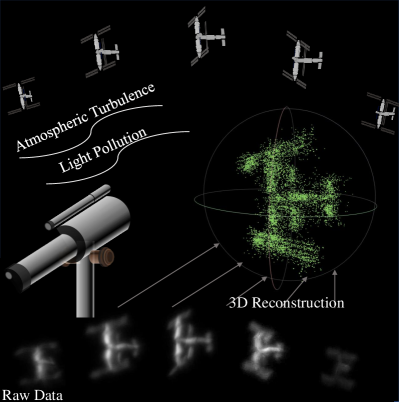
Figure 1: Problem definition. Our objective is to reconstruct a 3D model of a satellite in low-Earth orbit using limited, blurry, and noisy images captured by an amateur ground-based telescope, which are significantly affected by atmospheric turbulence and light pollution.

2 Related Work

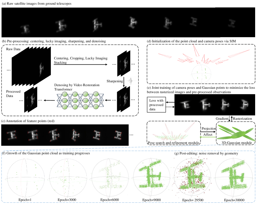
Figure 2: Overview of the 3D satellite reconstruction pipeline. This pipeline begins with the raw satellite images (a) obtained from ground-based telescopes, plagued by severe jitter, blurriness, and complex noise. Our methodology unfolds in three pivotal steps: 1) Image Pre-processing (b), which incorporates techniques such as centering, lucky imaging, wavelet decomposition sharpening, and deep learning denoising; 2) Joint 3D Reconstruction and Pose Estimation, covering the annotation of feature points (c), the initialization of the point cloud and camera poses (d), alongside simultaneous pose refinement (e) and 3D Gaussian training (f); 3) Point Cloud Post-editing (g), to refine and finalize the reconstructed 3D model.

2.1 Spaceborne 3D reconstruction and pose estimation

In space surveillance and servicing missions, such as satellite maintenance, debris removal, and formation flying, accurately estimating the pose of non-cooperative entities like spacecraft or debris is essential for safe and efficient operations. Monocular cameras stand out among pose estimation techniques for their low weight and power consumption, offering a simpler alternative to complex sensor systems such as differential GNSS[1], LiDAR, or stereo-vision cameras. However, applying conventional computer vision techniques [2, 3], originally designed for terrestrial environments, to space images poses significant challenges, given the simple textures, high noise levels, and symmetry commonly present in such images.

Deep learning has recently emerged as the leading method for spaceborne monocular pose estimation. This advancement has been significantly supported by the availability of open-source datasets of synthetic spacecraft images (e.g., SPEED[4], SPEED+[5], and SHIRT[6]), which are generated through computer graphics techniques. A variety of CNN-based methods[4, 7, 8, 9], developed and validated in ground-based flight testbeds simulating space-like conditions, have shown promising results. These CNN algorithms are further enhanced by incorporating 3D prior knowledge, such as point clouds[9] or wireframe models[10, 11], resulting in more robust pose estimation.

Despite these advances, much of the existing research relies on prior knowledge of the target’s structure and geometry, limiting its applicability to monitoring unknown space objects like debris. Recent developments are bridging vision-based pose estimation with 3D reconstruction to enable the characterization of uncharted spacecraft and asteroids[12, 13]. Leveraging extensive training on synthetic datasets, cutting-edge deep learning techniques are now capable of extracting both the shape and pose of unknown space objects from merely a single 2D image [14]. This progress marks a significant leap towards more versatile space surveillance capabilities.

2.2 NeRF and 3D Gaussian splatting

3D reconstruction is a critical area in computer vision, traditionally dominated by multi-view geometry process such as Structure from Motion (SFM)[15]. These methods typically extract feature descriptors (e.g., SIFT[16]) and establish correspondences between images using the RANSAC algorithm[17], followed by camera parameter estimation and point cloud generation through bundle adjustment[18]. Despite their effectiveness, they often struggle with capturing detailed textures, modeling complex lighting and sensor noise, and rendering new viewpoints accurately.

The advent of Neural Radiance Fields (NeRF)[19] introduced a paradigm shift in 3D reconstruction and view synthesis by using deep neural networks to model scenes’ volumetric density and color. NeRF stands out for its ability to generate high-quality images from limited viewpoints, delivering realistic renderings that handle complex lighting and transparency with finesse, and capturing scene details with exceptional accuracy. However, NeRF’s reliance on dense neural network architectures brings about substantial computational demands, slowing down both training and rendering processes. Moreover, NeRF does not offer an explicit scene representation, complicating straightforward scene editing tasks. To address these issues, significant efforts have been made to refine NeRF, aiming at accelerating the training[20] and rendering[21, 22, 23], enhancing the model’s interpretability and editability[24], and improving the precision of pose estimation[25, 26, 27, 28, 29].

More recently, the emergence of 3D Gaussian splatting techniques[30] has offered a promising alternative, noted for its rapid training, real-time rendering capabilities, and user-friendly editing features. 3D Gaussian splatting employs differentiable, splittable, and movable 3D Gaussian points, along with spherical harmonics derived from point clouds, to explicitly represent complex scenes. This explicit representation accelerates scene rendering compared to fully connected neural networks while simultaneously simplifying the process of scene editing[31, 32, 33], marking a significant evolution in the efficient manipulation and modification of reconstructed 3D environments.

2.3 Imaging through turbulence

Atmospheric turbulence significantly compromises image quality in ground-based telescope observations. For decades, efforts to address this challenge have led to the development of various mitigation techniques. One widely adopted approach is Adaptive Optics (AO) [34], which utilizes deformable mirrors to actively compensate for wavefront aberrations caused by atmospheric turbulence. However, the implementation of AO systems requires sophisticated and costly hardware, confining their use primarily to large astronomical observatories.

Classical algorithmic methods [35, 36, 37] for turbulence reduction often employ lucky imaging[38], a strategy of capturing multiple images and selecting those least affected by turbulence according to predefined image quality metrics. This technique capitalizes on the rare moments when atmospheric conditions yield clearer images. Recent advancements in rapid, physics-based turbulence simulators [39, 40, 41] have facilitated the rise of learning-based approaches[42, 43, 44, 45] as an effective alternative. By utilizing extensive datasets of turbulence-affected images, these approaches leverage neural networks to decipher and learn the intricate patterns of turbulence degradation. The ability to harness the power of deep learning and large-scale data enables these methods to surpass classical techniques, paving a new way for enhanced imaging through turbulence.

3 Method

This paper aims to accomplish the 3D reconstruction of space objects based on monocular images captured by a ground-based telescope. In contrast to common 3D reconstruction tasks in computer vision, ground-based telescope observations are significantly contaminated by atmospheric turbulence and light pollution, as shown in Fig.2(a). Turbulence disrupts light paths through the atmosphere, while light pollution from artificial sources reduces the visibility of celestial objects. Moreover, the fixed and limited viewpoints from the telescope introduce further complexity, resulting in a super challenging 3D reconstruction problem from constrained, distorted, blurry, and noisy images.

In response to these challenges, we propose a novel 3D reconstruction approach based on the cutting-edge Gaussian splatting algorithm. This approach encompasses three major steps: 1) pre-processing of raw telescope images (Fig.2(b)), 2) joint pose estimation and 3D Gaussian splatting reconstruction (Fig.2(c)-(f)), and 3) post-reconstruction editing of Gaussian point clouds (Fig.2(g)). The implementation details of each step are explained below.

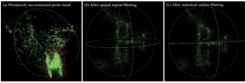
Figure 3: Post-editing significantly improves the accuracy of the reconstructed 3D model. (a) Primitively reconstructed point cloud amidst highly complex noise conditions, where red box indicates the region of satellite. (b) Point cloud after spatial region filtering. (c) Point cloud after statistical outlier filtering.

3.1 Pre-processing of Raw Telescope Images

Pre-processing raw images from ground telescopes is a critical first step to mitigate distortions and enhance image quality for subsequent reconstruction, as demonstrated in Fig.2(b). The pre-processing involves the following steps:

a) Centering and lucky imaging: To address distortion in telescope data, we initially apply lucky imaging to sequences of short-exposure raw images using image processing software like Autostakkert[46]. Lucky imaging consists of two main activities. The first involves ranking images by contrast and clarity to select a subset of high-quality frames. These selected frames represent moments least affected by the atmospheric turbulence and light pollution, thus identifying the sharpest images. The second involves registering and stacking these frames to increase the signal-to-noise ratio. Given that space targets often shift due to atmospheric dynamics and telescope instability, we center the images on their centroids before applying lucky imaging[47].

b) Image sharpening with wavelet decomposition: Although stacking improves signal clarity by reducing noise, it inevitably diminishes high-frequency details. To counteract this effect, we sharpen the stacked images by amplifying the high-frequency features through Gaussian wavelet decomposition, accomplished by using the public software RegiStax[48]. This process also helps diminish the background light pollution by attenuating low-frequency features.

c) Image enhancement with video restoration transformer: Image sharpening can introduce additional high-frequency noise or artifacts. To address this, we apply the state-of-the-art Video Restoration Transformer (VRT)[49], a foundational model for video processing pre-trained on extensive datasets, to further denoise the post-sharpening images.

3.2 Joint pose estimation and 3D reconstruction

In astrophotography, space objects orbit in high speed, whereas telescopes remain stationary on the Earth. For simplicity in adapting cutting-edge computer vision techniques, we simplify this dynamic by assuming the space object remains stationary and the telescope/camera moves around it for data acquisition. This process involves the following key steps:

a) Annotation of video’s feature points: We begin by manually annotating feature points on the satellite, such as the corners of a satellite’s solar wings, highlighted in red in Fig.2(c). Atmospheric distortion and the satellite’s geometric simplicity result in images with limited texture and blurred edge details. Consequently, feature extraction using standard and neural network-based detectors like SIFT[2] and SuperPoint[50, 51] proves unreliable, and manually annotating these points becomes necessary. We leave the automated feature point annotation for future work.

b) Initializing camera poses and 3D Gaussians with SfM: Following the identification of feature points, we employ the Structure from Motion (SfM)[15] algorithm to create an initial 3D point cloud of the target and determine the camera’s pose and focal length for each frame. These initial estimates are marked by red for poses and focal lengths and green for the point cloud in Fig.2(d). Given the long focal lengths of ground-based telescopes, we often encounter inaccuracies in camera-to-target distance estimation. To counter this, we refine our pose estimates utilizing satellite trajectory calculations informed by astrodynamics. In instances where poses cannot be determined due to unavailable or inaccurate feature point annotations—resulting in the failure of SfM convergence—we resort to interpolation to fill the missing values. Quadratic interpolation is applied for the camera’s translational vector, $T$, and spherical linear interpolation is used for the camera’s rotation matrix, $R$. The updated initialization is depicted in green in Fig.2(e).

c) Alternating between pose estimation and 3D reconstruction: The Gaussian splatting algorithm is then used for reconstructing the space object in 3D. To avoid overfitting, we carefully manage the growth of Gaussian points and concurrently update camera poses. Initially, we train the 3D Gaussians for 1,000 epochs, applying a loss function that combines L1 and SSIM metrics. Pose adjustments are then performed using the Branch and Bound (BnB)[52] algorithm, updating camera’s orientations and translations while fixing camera-to-target distances. We then alternate between updating 3D Gaussians and refining camera poses every 500 epochs, as depicted in Fig.2(f). Such iteration increases the number of Gaussian points progressively and gradually fits the point cloud to the target satellite. After completing 22 cycles (12,000 epochs), we stop point cloud growth (splitting) and pose adjustments, focusing solely on refining the parameters of existing Gaussian points until convergence after 30,000 epochs.

TABLE I: Comparison of our method and NeRF on five simulation datasets and on-sky observations of China’s Space Station. The optimal result in each column (with training and validation views considered separately) is highlighted in bold.

		Simulation 1			Simulation 2			Simulation 3			Simulation 4			Simulation 5			On-sky
	Method	PSNR$\uparrow$	SSIM$\uparrow$	LPIPS$\downarrow$	PSNR$\uparrow$	SSIM$\uparrow$	LPIPS$\downarrow$	PSNR$\uparrow$	SSIM$\uparrow$	LPIPS$\downarrow$	PSNR$\uparrow$	SSIM$\uparrow$	LPIPS$\downarrow$	PSNR$\uparrow$	SSIM$\uparrow$	LPIPS$\downarrow$	PSNR$\uparrow$	SSIM$\uparrow$	LPIPS$\downarrow$
Dirty Image		23.28	0.07	0.41	22.23	0.07	0.36	23.02	0.07	0.36	23.16	0.07	0.36	24.19	0.13	0.38	$\times$	$\times$	$\times$
Pre-Processed		27.60	0.53	0.10	26.71	0.55	0.12	27.92	0.53	0.11	28.3	0.52	0.11	23.08	0.54	0.29	$\times$	$\times$	$\times$
Train	Ours	26.44	0.92	0.10	24.88	0.91	0.16	27.30	0.92	0.14	27.69	0.91	0.10	25.47	0.92	0.15	36.97	0.98	0.01
	NeRF	25.39	0.65	0.13	19.10	0.61	0.19	25.00	0.62	0.15	26.97	0.64	0.12	23.21	0.67	0.18	36.60	0.97	0.03
Validation	Ours	26.32	0.92	0.10	24.65	0.90	0.16	27.12	0.91	0.14	27.51	0.91	0.11	25.38	0.92	0.16	36.80	0.98	0.01
	NeRF	17.42	0.55	0.36	17.15	0.56	0.33	21.40	0.59	0.20	22.64	0.60	0.19	21.40	0.65	0.21	23.21	0.67	0.18

3.3 Post-reconstruction editing of gaussian point clouds

The reconstructed 3D Gaussian point clouds often include stray points, as illustrated in Fig.3(a). These stray points come from the residual background noise and artifacts in the telescope images used in Gaussian splatting training. To achieve a cleaner reconstruction, we apply geometric filters to remove these outliers, employing two primary strategies. This step effectively capitalizes on the strengths of 3D Gaussian splatting in editability.

a) Spatial region filter: Acknowledging the compact structure of satellites, we begin the refinement process with a spatial region filter. This involves defining a spherical boundary around the target and discarding points outside this specified perimeter. Considering that solar wings usually mark the outermost boundary of a satellite, we set the radius of our spherical region to be 1.1 times the radius derived from the initial feature points at the corners of the solar wings. The center is placed at the mean position of these points. This process results in a more concentrated point cloud, as visualized in Fig.3(b).

b) Statistical outlier filter: We then implement a statistical outlier filter to eliminate isolated noise points—those significantly distant from their neighbors, as visualized in Fig. 3(c). This approach identifies outliers based on each point’s average distance to its $k$ nearest neighbors, $\bar{d_{i}}$. Given the mean ($\mu$) and standard deviation ($\sigma$) of these distances across the cloud, we set a threshold $\tau=\mu+\alpha\cdot\sigma$, where $\alpha$ is a multiplier (set to 1 in our method), and flag out points with $\bar{d_{i}}>\tau$.

After applying these filters, we resume Gaussian splatting training on the refined point cloud for an additional 500 epochs, repairing any discontinuities introduced by the filtering. This adjustment further enhances the overall quality of the reconstructed point cloud.

4 Experiments

In this section, we report the experiments conducted to evaluate our 3D reconstruction method, with NeRF serving as the benchmark for comparison. We utilized three standard imaging metrics—SSIM, PSNR, and LPIPS—on 2D views of the reconstructed volumes to gauge the reconstruction accuracy. Our method demonstrates superior reconstruction quality and robustness on both synthetic ground telescope satellite images and real observational data of China’s Space Station.

4.1 Simulation Results

Synthetic Ground Telescope Satellite Images  For simulation, we created five distinct 3D satellite models in Blender, an open-source 3D computer graphics software, and produced five datasets of corresponding ground telescope images. Each model is roughly 60 meters in size, positioned in a circular low-Earth orbit at approximately 650 kilometers altitude, equivalent to a radius of 7100 kilometers. Since the telescope is stationary on the Earth, it captures only a 13^∘ segment of the satellite’s full 360^∘ trajectory. Our virtual telescope, equipped with a 0.35-meter aperture and a 3.2-meter focal length, allowed us to render 700 high-quality images for each model. To simulate atmospheric conditions, 20 frames were perturbed for each original image, introducing effects of turbulence and light pollution, thus totaling 14,000 frames with distorted imagery. Turbulence in each frame varied, with a Fried parameter (coherence length) between 0.07 and 0.35 meters. Light pollution contributed an additional 5%-7% to the background intensity, measured against the satellite’s brightness. Our dataset will be made publicly available after the paper’s acceptance.

Implementation Details  In preprocessing the synthetic datasets, we fine-tuned the lucky imaging parameters to distill 148 clean images from a pool of 14,000 distorted frames. To evaluate the efficacy of our preprocessing workflow, we first assessed the improvements in image quality after the preprocessing step based on the Ground Truth images, with the results detailed in Table I. Subsequently, we selected one out of every ten clean frames, in total 15 frames, for Gaussian splatting or NeRF training, with the remaining images set aside for 3D reconstruction validation. The camera poses optimized through our combined approach of Gaussian splatting training and Branch and Bound (BnB) pose refinement were saved and employed in NeRF training. This ensured the elimination of pose estimation accuracy as a variable in performance differences observed between the methodologies.

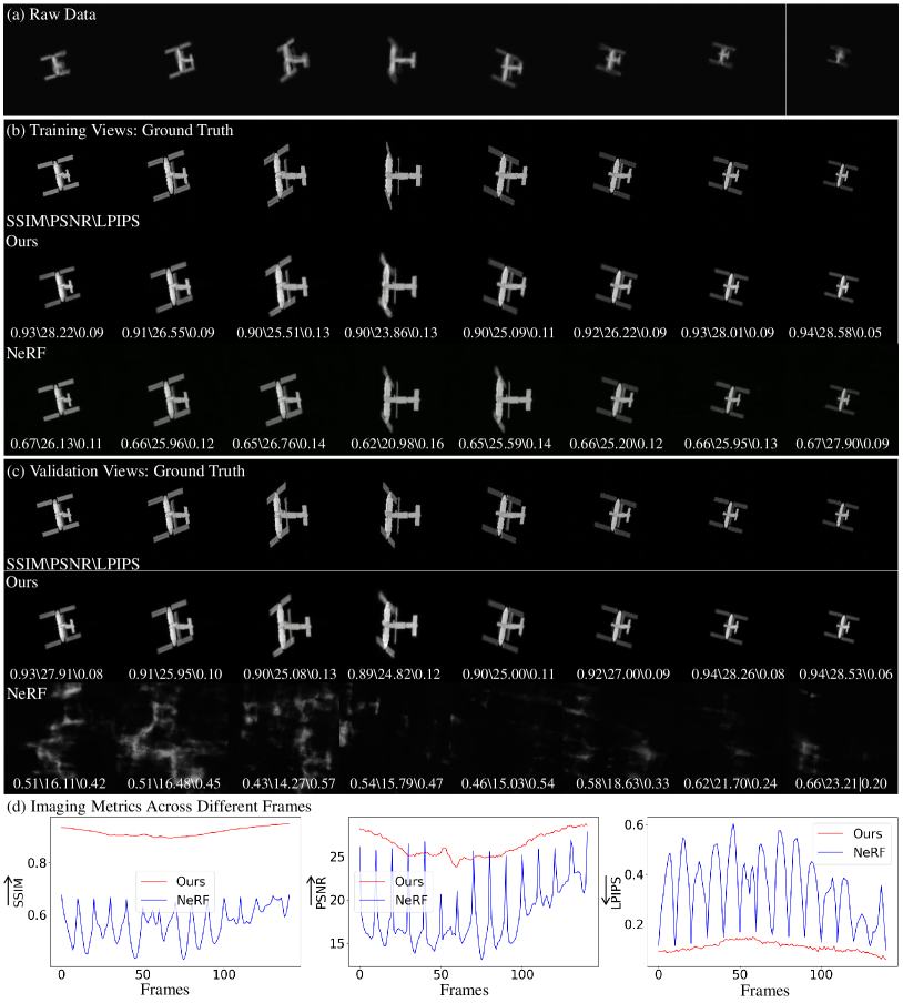
Figure 4: Results of 3D reconstruction and view synthesis for the 1st simulation dataset. (a) Simulated raw images featuring atmospheric turbulence, light pollution, and sensor noise. (b) Rendering quality comparison in training views between our method and NeRF. (c) Rendering quality comparison in validation views between our method and NeRF. (d) Imaging metrics evaluated across various frames, encompassing both training and validation views. Our method demonstrated outstanding precision in both training and validation views, while NeRF encountered difficulties in rendering unseen viewpoints.

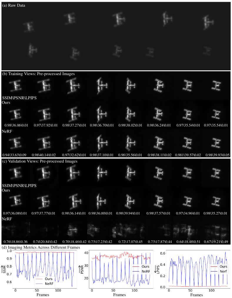
Figure 5: Results of 3D reconstruction and view synthesis for the China’s Space Station Observation. (a) Raw images from the amateur telescope. (b) Rendering quality comparison in training views between our method and NeRF. (c) Rendering quality comparison in validation views between our method and NeRF. (d) Imaging metrics evaluated across various frames, encompassing both training and validation views. The performance discrepancy between NeRF and our method becomes more significant.

3D Reconstruction  Figure.4 illustrates the results of 3D reconstruction for the first simulation dataset, comparing the performance of both NeRF and our method through selected views of the reconstructed volumes. NeRF reveals reasonable reconstruction quality in the training views (Fig.4(b)) but struggles when rendering novel viewpoints (Fig.4(c)) due to overfitting issues. In contrast, our method demonstrates superior generalization ability, excelling in both training and validation views. This indicates that our reconstructed 3D Gaussian point cloud precisely captures the satellites’ 3D shapes. The effectiveness of our method is also supported by the curves of image quality metrics (SSIM, PSNR, LPIPS) across various frames, illustrated in Fig.4(d). Extending this experiment to all five datasets, our technique consistently surpasses NeRF in all evaluated metrics, as presented in Table I. These findings affirm our approach’s efficiency and accuracy in 3D reconstruction challenges. We would also like to highlight that our method significantly outpaces NeRF in terms of training speed. It takes approximately 7 minutes to reconstruct a 3D volume with our approach on a single NVIDIA’s RTX 4090—around 3 minutes for Gaussian splatting training and an additional 4 minutes for BnB pose search. In contrast, training a basic NeRF model requires more than 4 hours.

4.2 On-Sky Results

We applied our algorithm to real observations of China’s Tiangong Space Station, a low-Earth-orbit satellite with publicly available geometric specifications.

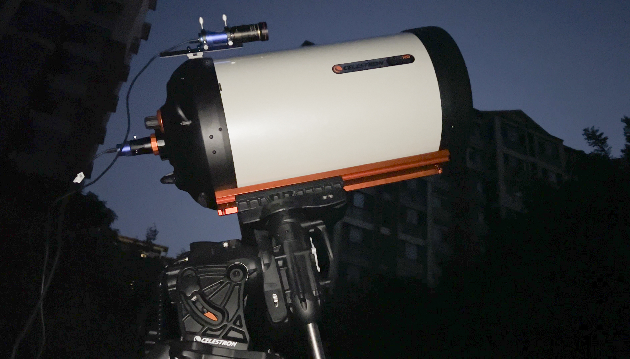
Figure 6: Imaging Instrument: the Celestron C14HD telescope paired with a QHY5III678M planetary camera.

Observation of China’s Tiangong Space Station  The observation took place on September 15, 2023, during a pass of the Tiangong Station from 20:48:30 to 20:51:17 (UTC).

The observation site is situated near Miyun Observatory on the northern bank of Miyun Reservoir, Beijing, China, chosen for its advantageous seeing conditions. The Tiangong Station was 389.4 km away at its closest, reaching a maximum elevation of 78.3 degrees. We used a Celestron C14HD telescope (0.35m diameter, f/11) paired with a QHY5III678M planetary camera for this observation. This setup, with a telescope focal length of 3.91 meters and a camera pixel pitch of 2 micrometers, provided a spatial sampling rate of 0.106 arcsec/pixel, enabling us to image the Tiangong Station at 0.2 m/pixel resolution at its nearest point.

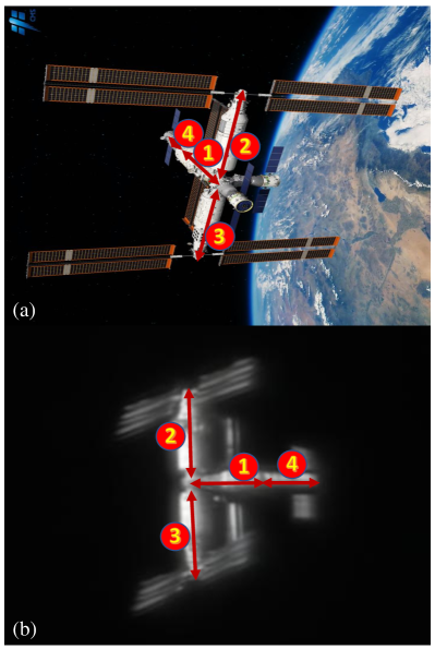
Figure 7: Composition of the Chinese Space Station (CSS). The CSS comprises four primary modules: 1 - Tianhe Core Module, 2 - Mengtian Laboratory Module, 3 - Wentian Laboratory Module, 4 - Tianzhou-6 Cargo Spacecraft. (a) An official image of the CSS. (b) A rendering derived from our 3D reconstruction of the CSS.

TABLE II: Metrology of the China’s Space Station modules and their solar wings.

	Measured Value	Ground Truth[53]
Solar wing angle
Tianhe Core Module	0.78	$\times$
Mengtian Laboratory Module	63.01	$\times$
Wentian Laboratory Module	68.71	$\times$
Tianzhou-6	3.22	$\times$
Length
Tianhe Core Module	16.11	16.6
Mengtian Laboratory	17.30	17.88
Wentian Laboratory	17.30	17.88
Tianzhou-6	9.71	10.6
Diameter
Tianhe Core Module	5.65	4.2
Mengtian Module	5.50	4.2
Wentian Module	5.63	4.2
Tianzhou 6	3.30	3.35
The length of the solar wings
Tianhe Core Module	25.44	$\times$
Mengtian Laboratory Module	55.62	55
Wentian Laboratory Module	55.62	55
Tianzhou 6	4.89	$\times$

TABLE III: Ablation study on five simulated data. For clarity, the optimal result in each column (with training and validation views considered separately) is highlighted in bold, while the next best result is underlined.

		Simulation 1			Simulation 2			Simulation 3			Simulation 4			Simulation 5
	Method	PSNR$\uparrow$	SSIM$\uparrow$	LPIPS$\downarrow$	PSNR$\uparrow$	SSIM$\uparrow$	LPIPS$\downarrow$	PSNR$\uparrow$	SSIM$\uparrow$	LPIPS$\downarrow$	PSNR$\uparrow$	SSIM$\uparrow$	LPIPS$\downarrow$	PSNR$\uparrow$	SSIM$\uparrow$	LPIPS$\downarrow$
Train	Ours	26.44	0.92	0.10	24.88	0.91	0.16	27.30	0.92	0.14	27.69	0.91	0.10	25.47	0.92	0.15
	No Sharpening	24.22	0.90	0.15	24.34	0.54	0.20	25.91	0.90	0.16	27.63	0.90	0.17	24.42	0.80	0.15
	No Gaussian initialization	24.03	0.62	0.17	16.59	0.88	0.29	24.41	0.62	0.15	19.74	0.87	0.23	22.77	0.68	0.19
	No pose refinement	22.86	0.85	0.17	18.47	0.79	0.20	17.56	0.78	0.24	24.77	0.82	0.17	19.22	0.84	0.20
	No Regulation of Gaussian	21.78	0.86	0.15	18.41	0.82	0.23	23.55	0.87	0.14	23.14	0.69	0.18	22.66	0.87	0.16
	No Point cloud Filtering	27.86	0.64	0.11	25.76	0.63	0.16	27.38	0.64	0.14	28.00	0.62	0.10	25.82	0.70	0.15
Validation	Ours	26.32	0.91	0.10	24.65	0.90	0.16	27.12	0.91	0.14	27.51	0.91	0.11	25.38	0.92	0.16
	No Sharpening	24.12	0.90	0.15	23.92	0.52	0.20	25.78	0.90	0.17	27.43	0.90	0.17	23.99	0.80	0.15
	No Gaussian initialization	19.48	0.50	0.23	16.37	0.78	0.30	19.91	0.50	0.23	18.77	0.77	0.26	17.34	0.53	0.27
	No pose refinement	22.85	0.85	0.17	18.39	0.78	0.20	17.39	0.78	0.24	24.34	0.81	0.18	19.09	0.84	0.20
	No Regulation of Gaussian	21.72	0.86	0.15	17.71	0.80	0.25	22.24	0.85	0.15	21.99	0.68	0.20	21.39	0.85	0.16
	No Point cloud Filtering	27.55	0.64	0.11	25.39	0.63	0.16	27.16	0.64	0.14	27.70	0.62	0.11	25.57	0.69	0.15

The observation utilized the ”Fake Polar Axis Method” with a German-type equatorial mount (CGX-L), uniquely oriented not towards the north but towards a precisely calculated azimuth relative to the apparent track of the space object. This innovative method prevented the need for a meridian flip during the observation and minimized field rotation, particularly beneficial for the central part of the image sequence. During the 166-second observation period, we captured images at an average rate of 87.8 fps with 5-millisecond exposures. However, due to cache degradation, the frame rate varied, starting higher at 93.5 fps and decreasing towards the end. This resulted in a dataset of 13,800 raw images.

Implementation Details  Employing lucky imaging techniques, we obtained 157 frames from the inital pool of 13,800 dirty images. By further filtering out images plagued by exceptionally low signal-to-noise ratios, we finalized a set of 138 clean frames. Consistent with the strategy of our simulation experiments, we selected one image for every ten frames for reconstruction training, totaling 15 images. The remaining images were allocated to the validation set. For each selected training image, we recorded the optimized camera poses and conducted a parallel reconstruction with NeRF using identical poses. Due to the lack of ground-truth images in on-sky experiments, we assessed imaging metrics by directly comparing the reconstruction outcomes with the pre-processed images.

3D Reconstruction and Metrology  The 3D reconstruction outcomes for the Tiangong dataset, as shown in Fig.5, echo our simulation findings—NeRF struggled with rendering unseen views, highlighting its challenges in accurately capturing the satellite’s 3D structure. In contrast, our approach achieved exceptional 3D reconstruction precision across both training and validation views, with the performance discrepancy between NeRF and our method being notably more pronounced in this real-world dataset than in simulation scenarios. This contrast in image quality metrics is further elaborated in the last column of Table I.

Additionally, we performed detailed measurements on four modules of the space station (Tianhe, Mengtian, Wentian, and Tianzhou-6) and the angles and lengths of their solar wings, utilizing our 3D Gaussian splatting-reconstructed volume, as illustrated in Fig.7. To measure the modules’ sizes (length and diameter), we densely sampled 2D views, pinpointing the frames that depicted each module at its maximum length (from orthogonal perspectives) and determining dimensions via pixel counts. The angles of the solar wings were ascertained based on their relative positioning to the station’s main modules. These metrology findings, outlined in Table II, align closely with the officially released specifications

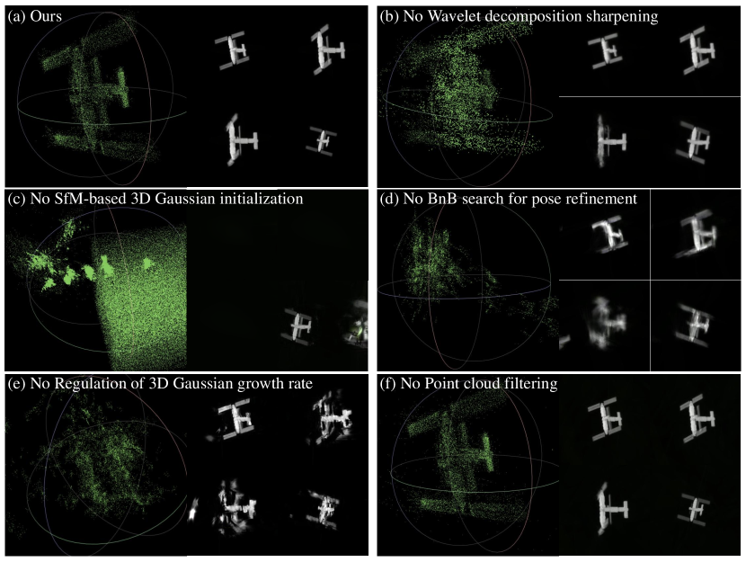
Figure 8: Ablation studies on the 1st simulation dataset. This figure showcases the impact of each component in our workflow on the reconstructed point clouds and novel view synthesis. (a) Results using our complete method. (b) Excluding wavelet decomposition image sharpening results in a blurry reconstruction. (c) Excluding SfM-based 3D Gaussian initialization introduces ghosting effects. (d) Excluding simultaneous pose refinement causes distortions and artifacts. (e) Excluding the regulation of 3D Gaussian growth rate also leads to distortions and artifacts. (f) Without point cloud post-editing, the background remains cluttered and noisy.

4.3 Ablation Study

Comprehensive ablation studies were carried out to ascertain the necessity of each element within our 3D reconstruction framework. Fig.8 showcases the consequences of excluding particular components from our pipeline, displaying the reconstructed points on the left and representative rendered views on the right for each subplot. From the top-left to the bottom-right in Fig.8(b)-(f), the components omitted are wavelet decomposition sharpening (Sec.3.1.b), SfM-based 3D Gaussian initialization (Sec.3.2.b), BnB search for pose refinement (Sec.3.2.c), regulation of 3D Gaussian growth rate (Sec.3.2.c, splitting large Gaussians every 100 epochs instead of 500 epochs), and point cloud filtering (Sec.3.3). The exclusion of these steps visibly impairs the reconstruction outcome, manifesting as blurriness, ghosting, fringe artifacts, and unclean backgrounds, among other issues. Furthermore, Table III details the quantitative results of these ablation studies, underscoring the degradation in reconstruction quality when vital steps are skipped. The ablation results for lucky imaging (Sec.3.1.a) and feature annotation (Sec.3.2.a) are not presented, as omitting these steps resulted in the inability to reconstruct anything.

5 Conclusion

In this paper, we introduced a novel 3D imaging framework designed for reconstructing satellites from ground telescope observations. Central to this approach is the utilization of the cutting-edge Gaussian splatting volume rendering algorithm, complemented by sophisticated pre-processing, simultaneous pose refinement, and post-editing techniques to effectively manage the significant image distortions caused by atmospheric turbulence, light pollution, and other factors. We validated our method using both synthetic datasets and actual observations of China’s Tiangong Space Station.

A notable limitation of our current methodology is the need for manual annotation of feature points, a step necessitated by the considerable ambiguity present in raw telescope images. Future efforts will focus on addressing this challenge by developing a feature extraction neural network specifically designed for imaging through turbulence scenarios. We aim to finally establish a fully automated end-to-end workflow from video capture to 3D model generation.

We believe the insights from this research can significantly benefit 3D reconstruction tasks across various scientific fields facing complex image distortions. Potential applications include, for example, remote sensing, biomedical ultrasound/photoacoustic imaging and deep tissue imaging in microscopy.

References

- [1] V. Giralo and S. D’Amico, “Distributed multi-gnss timing and localization for nanosatellites,” Navigation, vol. 66, no. 4, pp. 729–746, 2019.
- [2] D. G. Lowe, “Distinctive image features from scale-invariant keypoints,” International journal of computer vision, vol. 60, pp. 91–110, 2004.
- [3] S. Sharma et al., “Comparative assessment of techniques for initial pose estimation using monocular vision,” Acta Astronautica, vol. 123, pp. 435–445, 2016.
- [4] S. Sharma and S. D’Amico, “Neural network-based pose estimation for noncooperative spacecraft rendezvous,” IEEE Transactions on Aerospace and Electronic Systems, vol. 56, no. 6, pp. 4638–4658, 2020.
- [5] T. H. Park, M. Märtens, G. Lecuyer, D. Izzo, and S. D’Amico, “Speed+: Next-generation dataset for spacecraft pose estimation across domain gap,” in 2022 IEEE Aerospace Conference (AERO). IEEE, 2022, pp. 1–15.
- [6] T. H. Park and S. D’Amico, “Adaptive neural-network-based unscented kalman filter for robust pose tracking of noncooperative spacecraft,” Journal of Guidance, Control, and Dynamics, vol. 46, no. 9, pp. 1671–1688, 2023.
- [7] ——, “Robust multi-task learning and online refinement for spacecraft pose estimation across domain gap,” Advances in Space Research, 2023.
- [8] X. Zhang, Z. Jiang, H. Zhang, and Q. Wei, “Vision-based pose estimation for textureless space objects by contour points matching,” IEEE Transactions on Aerospace and Electronic Systems, vol. 54, no. 5, pp. 2342–2355, 2018.
- [9] S. Qiao, H. Zhang, G. Meng, M. An, F. Xie, and Z. Jiang, “Deep-learning-based satellite relative pose estimation using monocular optical images and 3d structural information,” Aerospace, vol. 9, no. 12, p. 768, 2022.
- [10] S. Sharma, J. Ventura, and S. D’Amico, “Robust model-based monocular pose initialization for noncooperative spacecraft rendezvous,” Journal of Spacecraft and Rockets, vol. 55, no. 6, pp. 1414–1429, 2018.
- [11] S. D’Amico, M. Benn, and J. L. Jørgensen, “Pose estimation of an uncooperative spacecraft from actual space imagery,” International Journal of Space Science and Engineering 5, vol. 2, no. 2, pp. 171–189, 2014.
- [12] H. Zhang, Q. Wei, and Z. Jiang, “3d reconstruction of space objects from multi-views by a visible sensor,” Sensors, vol. 17, no. 7, p. 1689, 2017.
- [13] K. Dennison and S. D’Amico, “Vision-based 3d reconstruction for navigation and characterization of unknown, space-borne targets,” Austin, TX, Jan, 2023.
- [14] T. H. Park and S. D’Amico, “Rapid abstraction of spacecraft 3d structure from single 2d image,” in AIAA SCITECH 2024 Forum, 2024, p. 2768.
- [15] J. L. Schonberger and J.-M. Frahm, “Structure-from-motion revisited,” in Proceedings of the IEEE conference on computer vision and pattern recognition, 2016, pp. 4104–4113.
- [16] D. G. Lowe, “Object recognition from local scale-invariant features,” in Proceedings of the seventh IEEE international conference on computer vision, vol. 2. Ieee, 1999, pp. 1150–1157.
- [17] M. A. Fischler and R. C. Bolles, “Random sample consensus: a paradigm for model fitting with applications to image analysis and automated cartography,” Communications of the ACM, vol. 24, no. 6, pp. 381–395, 1981.
- [18] B. Triggs, P. F. McLauchlan, R. I. Hartley, and A. W. Fitzgibbon, “Bundle adjustment—a modern synthesis,” in Vision Algorithms: Theory and Practice: International Workshop on Vision Algorithms Corfu, Greece, September 21–22, 1999 Proceedings. Springer, 2000, pp. 298–372.
- [19] B. Mildenhall, P. P. Srinivasan, M. Tancik, J. T. Barron, R. Ramamoorthi, and R. Ng, “Nerf: Representing scenes as neural radiance fields for view synthesis,” Communications of the ACM, vol. 65, no. 1, pp. 99–106, 2021.
- [20] T. Müller, A. Evans, C. Schied, and A. Keller, “Instant neural graphics primitives with a multiresolution hash encoding,” ACM Trans. Graph., vol. 41, no. 4, pp. 102:1–102:15, Jul. 2022. [Online]. Available: https://doi.org/10.1145/3528223.3530127
- [21] A. Chen, Z. Xu, A. Geiger, J. Yu, and H. Su, “Tensorf: Tensorial radiance fields,” in European Conference on Computer Vision (ECCV), 2022.
- [22] S. Fridovich-Keil, G. Meanti, F. R. Warburg, B. Recht, and A. Kanazawa, “K-planes: Explicit radiance fields in space, time, and appearance,” in Proceedings of the IEEE/CVF Conference on Computer Vision and Pattern Recognition, 2023, pp. 12 479–12 488.
- [23] A. Cao and J. Johnson, “Hexplane: A fast representation for dynamic scenes,” in Proceedings of the IEEE/CVF Conference on Computer Vision and Pattern Recognition, 2023, pp. 130–141.
- [24] V. Lazova, V. Guzov, K. Olszewski, S. Tulyakov, and G. Pons-Moll, “Control-nerf: Editable feature volumes for scene rendering and manipulation,” in Proceedings of the IEEE/CVF Winter Conference on Applications of Computer Vision, 2023, pp. 4340–4350.
- [25] Z. Wang, S. Wu, W. Xie, M. Chen, and V. A. Prisacariu, “Nerf–: Neural radiance fields without known camera parameters,” arXiv preprint arXiv:2102.07064, 2021.
- [26] Y. Chen, X. Chen, X. Wang, Q. Zhang, Y. Guo, Y. Shan, and F. Wang, “Local-to-global registration for bundle-adjusting neural radiance fields,” in Proceedings of the IEEE/CVF Conference on Computer Vision and Pattern Recognition, 2023, pp. 8264–8273.
- [27] C.-H. Lin, W.-C. Ma, A. Torralba, and S. Lucey, “Barf: Bundle-adjusting neural radiance fields,” in Proceedings of the IEEE/CVF International Conference on Computer Vision, 2021, pp. 5741–5751.
- [28] W. Bian, Z. Wang, K. Li, J.-W. Bian, and V. A. Prisacariu, “Nope-nerf: Optimising neural radiance field with no pose prior,” in Proceedings of the IEEE/CVF Conference on Computer Vision and Pattern Recognition, 2023, pp. 4160–4169.
- [29] K. Park, P. Henzler, B. Mildenhall, J. T. Barron, and R. Martin-Brualla, “Camp: Camera preconditioning for neural radiance fields,” ACM Transactions on Graphics (TOG), vol. 42, no. 6, pp. 1–11, 2023.
- [30] B. Kerbl, G. Kopanas, T. Leimkühler, and G. Drettakis, “3d gaussian splatting for real-time radiance field rendering,” ACM Transactions on Graphics, vol. 42, no. 4, 2023.
- [31] Y. Chen, Z. Chen, C. Zhang, F. Wang, X. Yang, Y. Wang, Z. Cai, L. Yang, H. Liu, and G. Lin, “Gaussianeditor: Swift and controllable 3d editing with gaussian splatting,” arXiv preprint arXiv:2311.14521, 2023.
- [32] J. Fang, J. Wang, X. Zhang, L. Xie, and Q. Tian, “Gaussianeditor: Editing 3d gaussians delicately with text instructions,” arXiv preprint arXiv:2311.16037, 2023.
- [33] J. Huang and H. Yu, “Point’n move: Interactive scene object manipulation on gaussian splatting radiance fields,” arXiv preprint arXiv:2311.16737, 2023.
- [34] F. Roddier, “Adaptive optics in astronomy,” 1999.
- [35] N. Anantrasirichai, A. Achim, and D. Bull, “Atmospheric turbulence mitigation for sequences with moving objects using recursive image fusion,” in IEEE international conference on image processing, 2018, pp. 2895–2899.
- [36] N. Anantrasirichai, A. Achim, N. G. Kingsbury, and D. R. Bull, “Atmospheric turbulence mitigation using complex wavelet-based fusion,” IEEE Transactions on Image Processing, vol. 22, no. 6, pp. 2398–2408, 2013.
- [37] Z. Mao, N. Chimitt, and S. H. Chan, “Image reconstruction of static and dynamic scenes through anisoplanatic turbulence,” IEEE Transactions on Computational Imaging, vol. 6, pp. 1415–1428, 2020.
- [38] N. M. Law, C. D. Mackay, and J. E. Baldwin, “Lucky imaging: high angular resolution imaging in the visible from the ground,” Astronomy & Astrophysics, vol. 446, no. 2, pp. 739–745, 2006.
- [39] A. Schwartzman, M. Alterman, R. Zamir, and Y. Y. Schechner, “Turbulence-induced 2d correlated image distortion,” in IEEE International Conference on Computational Photography, 2017, pp. 1–13.
- [40] Z. Mao, N. Chimitt, and S. H. Chan, “Accelerating atmospheric turbulence simulation via learned phase-to-space transform,” in Proceedings of the IEEE/CVF International Conference on Computer Vision, 2021, pp. 14 759–14 768.
- [41] N. Chimitt, X. Zhang, Z. Mao, and S. H. Chan, “Real-time dense field phase-to-space simulation of imaging through atmospheric turbulence,” IEEE Transactions on Computational Imaging, vol. 8, pp. 1159–1169, 2022.
- [42] X. Zhang, N. Chimitt, Y. Chi, Z. Mao, and S. H. Chan, “Spatio-temporal turbulence mitigation: A translational perspective,” arXiv preprint arXiv:2401.04244, 2024.
- [43] R. Yasarla and V. M. Patel, “Learning to restore images degraded by atmospheric turbulence using uncertainty,” in 2021 IEEE International Conference on Image Processing, 2021, pp. 1694–1698.
- [44] S. N. Rai and C. Jawahar, “Removing atmospheric turbulence via deep adversarial learning,” IEEE Transactions on Image Processing, vol. 31, pp. 2633–2646, 2022.
- [45] K. Mei and V. M. Patel, “Ltt-gan: Looking through turbulence by inverting gans,” IEEE Journal of Selected Topics in Signal Processing, 2023.
- [46] E. Kraaikamp, “Autostakkert!” Software available from AutoStakkert website, 2024, accessed: 2024-03-20. [Online]. Available: https://www.autostakkert.com/
- [47] C. Garry, “Pipp: Planetary imaging preprocessor,” https://sites.google.com/site/astropipp/, 2014, version 2.3.8.
- [48] C. Berrevoets, “Registax 6,” http://www.astronomie.be/registax/, 2011, version 6.1.0.8.
- [49] J. Liang, J. Cao, Y. Fan, K. Zhang, R. Ranjan, Y. Li, R. Timofte, and L. Van Gool, “Vrt: A video restoration transformer,” arXiv preprint arXiv:2201.12288, 2022.
- [50] D. DeTone, T. Malisiewicz, and A. Rabinovich, “Superpoint: Self-supervised interest point detection and description,” in Proceedings of the IEEE conference on computer vision and pattern recognition workshops, 2018, pp. 224–236.
- [51] P.-E. Sarlin, D. DeTone, T. Malisiewicz, and A. Rabinovich, “Superglue: Learning feature matching with graph neural networks,” in Proceedings of the IEEE/CVF conference on computer vision and pattern recognition, 2020, pp. 4938–4947.
- [52] A. H. Land and A. G. Doig, An automatic method for solving discrete programming problems. Springer, 2010.
- [53] Wikipedia, “Tiangong space station,” 2024, [Online; accessed 28-March-2024]. [Online]. Available: https://en.wikipedia.org/wiki/Tiangong_space_station